Impact of inflow conditions and turbine placement on the performance of offshore wind turbines exceeding 7 MW

Accurately assessing wind turbine performance in large offshore wind farms requires a nuanced understanding of how inflow parameters, turbulence intensity (TI), wind shear, and wind veer are associated with power production across different turbine rows. In this study, we analyze 13 months of 10 min operational data from more than 40 high-capacity turbines in a North Sea offshore wind farm, complemented by nacelle-based lidar measurements used as an inflow proxy. Our objectives are to (1) quantify how power production differs between the front, middle, and rear sections of the farm under varying TI, shear, and veer and (2) evaluate the effectiveness of International Electrotechnical Commission (IEC)-based normalization methods, including rotor equivalent wind speed (REWS) and turbulence corrections, for both front-row and in-farm conditions.

The results indicate that the relationships between wind shear/veer and power output depend strongly on turbine location: upwind shear and veer correlate negatively with active power deviation in the front row but show positive correlations in the middle and rear rows. In addition, TI in the wake region has a distinct influence on power production, particularly at lower wind speeds, relative to TI observed in the front row. Finally, the rear section of the wind farm exhibits approximately 30 % lower variability in active power relative to the front section. These location-specific changes underscore the evolving nature of inflow conditions within large wind farms. Furthermore, IEC-based REWS may not fully capture the effects of shear and veer in large-scale offshore wind farms. Overall, the findings indicate that turbines operating in waked conditions may require additional inflow-characterization parameters beyond standard IEC norms to enable more accurate performance evaluations and support farm-level efficiency improvements.

To our knowledge, this study provides one of the first empirical assessments spanning the front, middle, and rear sections of a modern offshore wind farm to evaluate IEC-based REWS and TI normalizations, revealing location- and regime-dependent limitations and motivating complementary inflow descriptors for wake-affected operation.

1 Introduction

Global wind energy capacity continues to grow at an unprecedented rate, with new installations reaching 123 GW (World Wind Energy Association, 2024) worldwide in 2024, largely driven by robust climate policy commitments such as the EU REPowerEU Plan (European Commission, 2022) and the US Inflation Reduction Act (U.S. Congress, 2022). Although this expansion brings the international community closer to meeting ambitious decarbonization targets, it also underscores a host of technical and economic challenges. Among these are the high costs of operations and maintenance (O&M), particularly in offshore projects, and the need to optimize the power production of turbines that are increasing in size (Ren et al., 2021).

Today, onshore wind turbines frequently exceed 4 MW in capacity, while offshore machines of 8 MW or more are becoming increasingly common (Wiser et al., 2024; McCoy et al., 2024; Rohrig et al., 2019; Kelly and van der Laan, 2023). Factors such as turbulence intensity (TI), air density, wind shear, wind veer, and atmospheric stability significantly influence both their power output and their structural loading (Dimitrov et al., 2015; Martin et al., 2020; Sumner and Masson, 2006). Although larger turbines offer higher rated capacities and energy yields, their sensitivity to variations in inflow conditions can differ compared to smaller ones. For example, Chamorro et al. (2015) demonstrated that only turbulent structures exceeding the rotor diameter can substantially affect power output, while (Van Sark et al., 2019) showed that only wind turbines with a large rotor diameter to hub-height ratio can be significantly influenced by wind shear.

Although inflow effects have been studied numerically for both free-stream and wake conditions (Saint-Drenan et al., 2020; Sebastiani et al., 2023, 2024), most studies based on operational data have mainly focused on small- to medium-sized turbines (1.5–4 MW) operating in relatively undisturbed wind conditions (Gottschall and Peinke, 2008; Wagner et al., 2009; Murphy et al., 2020; Clifton and Wagner, 2014; Bardal and Sætran, 2017; Kim et al., 2021; Mata et al., 2024; Gao et al., 2021; Wagner et al., 2011). Many studies explore the effect of wakes on power production from the perspective of a velocity deficit (Adaramola and Krogstad, 2011; González-Longatt et al., 2012), but relatively few investigate the power performance of wind turbines within wind farms under waked conditions. Consequently, while turbines inside wind farms often experience inflow conditions that deviate significantly from free-stream, the impact of these deviations on power production remains relatively unexplored. Most prior studies treat wake effects primarily as mean-flow (velocity) deficits and evaluate power fluctuations with respect to a free-stream reference (e.g., for resource/AEP interpretations where farm-scale induction effects such as global blockage are treated as a bias). For example, Seifert et al. (2021) show that the standard deviation of the power increases with row index. In this study we condition on the local SCADA hub-height wind speed and quantify within-bin variability using identical IEC-style wind speed bins, enabling comparisons between regions of the wind farm that are not driven by differences in mean wind speed. Throughout, performance is evaluated conditionally on locally observed operating conditions (SCADA hub-height wind speed and the upstream-profile proxy), rather than relative to a reconstructed undisturbed free-stream reference.

Industry-standard normalization procedures for evaluating wind turbine performance are outlined by the International Electrotechnical Commission (IEC) (IEC, 2022). These methods correct for environmental factors such as TI, air density, wind shear, and veer and are widely used to compare the performance of different turbines under various conditions. However, they were developed primarily with single, isolated turbines in mind, and their applicability to the wake-affected regions of large wind farms is not recommended and has not yet been explored. Indeed, recent work suggests that standard IEC-based turbulence corrections can both overcompensate and undercompensate for inflow TI, potentially leading to inaccuracies in power curve estimates (Lee et al., 2020).

To address these gaps, this study aims to answer three questions. (Q1) How do inflow parameters, TI, shear, and veer affect power production across the front, middle, and rear sections of a modern offshore wind farm with turbines exceeding 7 MW? (Q2) How does short-term power variability differ across these sections? (Q3) To what extent do IEC normalization methods (REWS and the TI correction) mitigate these inflow dependencies in both free-stream and wake-affected conditions?

We test three hypotheses: (H1) the coupling between inflow descriptors (TI, shear, veer) and power production is location dependent within the farm (front vs. middle vs. rear); (H2) IEC-style normalizations (REWS for shear/veer and the TI correction) reduce apparent coupling near free-stream conditions but are insufficient or regime dependent in wake-affected rows; and (H3) wake-induced TI differs in effect from free-stream TI, especially below rated, leading to distinct correlation patterns and sensitivities across sections. Using 13 months of SCADA and upstream lidar wind speed profiles, we evaluate how the IEC normalization procedures behave in free-stream and wake-affected sections of a modern offshore wind farm.

This study provides three contributions: (i) a section-by-section (front/middle/rear) empirical analysis of how TI, shear, and veer correlate with power; (ii) a direct, within-farm evaluation of IEC normalizations (REWS, TI) that quantifies pre-/post-correction changes; and (iii) evidence that downstream rows exhibit lower power variability, measured via the median absolute deviation (MAD), and different TI coupling, motivating the need for inflow descriptors beyond current IEC parameters for wake-affected wind turbines.

The paper is organized as follows. Section 2 describes the datasets and filtering methods. Section 3 outlines the methodology, including the selection of specific sections of the wind farm, the corrections implemented, the correlation analyses conducted, and the variability analysis. Section 4 presents our results, examining each of the three corrections individually. Finally, Section 5 summarizes and discusses the key findings.

2 Data collection and filtering

The study uses 13 months of data from an offshore wind farm located within the Belgian maritime area. This wind farm comprises over 40 turbines positioned more than 30 km from the coastline. The prevailing wind direction is from the southwest, which predominantly influences the performance of the wind farm.

For the analysis, two different datasets are used:

• SCADA data. These data are collected from the wind turbines, providing real-time operational information. This includes wind speed, active power, TI, and direction measured by the SCADA system using a combination of cup anemometers, wind vanes, and sonic anemometers mounted on each turbine’s nacelle. The SCADA “rotor wind speed” is treated as the nacelle (hub-height) wind speed and denoted by v. For each 10 min interval, TI is computed as

  $$\mathrm{TI}={\displaystyle \frac{{\mathit{\sigma }}_v}{\stackrel{\mathrm{‾}}{v}}},$$

  where σ_v and $\stackrel{\mathrm{‾}}{v}$ are the standard deviation and mean of v over that interval. In the following, wind speeds shown in the figures as “normalized wind speed” correspond to the non-dimensional ratio

  $$\widehat{v}={\displaystyle \frac{v}{v_{\mathrm{rated}}}},$$

  with v_rated being the manufacturer rated wind speed of the wind turbine.

• Lidar data. A nacelle-mounted, continuous-wave (CW) ZX TM nacelle lidar (ZX Lidars) installed at a nearby wind farm at a distance of 23.5 km (see Fig. 1) delivers two line-of-sight (LOS) speeds at six heights per profile. LOS focus is set at approximately 2 rotor diameters upstream (≈420 m) to limit local induction effects from the host turbine. Lidar profiles are smoothed with a centered 30 min rolling window and evaluated at a 10 min cadence to match SCADA. To account for the large lidar–farm separation, the lidar time series are shifted by an advection delay

  $${\mathit{\tau }}_{jk}={\displaystyle \frac{s_{jk}}{U_{jk}^{\mathrm{adv}}}},$$

  where s_jk is the streamwise separation from the lidar focus to turbine k at time window j, and $U_j^{\mathrm{adv}}$ is the centered 30 min rolling mean of the lidar-measured wind speed over the same window.

2.1 Data filtering

Several filtering steps are applied to the combined dataset to ensure data validity:

1. Data availability. Data from 1 s measurements are aggregated into 10 min averages, allowing up to 100 s of missing data per 10 min window. This tolerance increased data availability without significantly impacting the uncertainty of the aggregated values.

2. Turbine operational regime and environmental dynamics. To ensure consistent operating conditions and wake interactions across the wind farm, a 10 min interval is kept only when all turbines are operating simultaneously. Data periods during which any of the studied turbines reported a fault or were curtailed for extended periods due to maintenance were excluded from the dataset. However, short-term operational curtailments, which are part of the normal control strategy of a large wind farm, were not filtered out. These events occur primarily at wind speeds above the rated power, a region of less focus for this study, and their inclusion ensures that the analysis remains representative of realistic farm-wide operating conditions. Beyond these operational filters, we intentionally retain dynamic atmospheric periods by foregoing an explicit stationarity filter (i.e., no ramp/gust screening). This ensures that the dataset reflects the operating conditions actually experienced by the farm and guards against overstating relationships based on selectively filtered periods.

3. Data sanity.

   • Low variability. The 10 min intervals, where the standard deviation of wind speed or active power was less than 0.01 % of its mean value, are removed to eliminate erroneous data points marked as rejected data.

   • Outliers (HDBSCAN). Operating states inconsistent with the nominal power curve are removed using hierarchical density-based spatial clustering of applications with noise (HDBSCAN) (McInnes et al., 2017) in a two-dimensional space defined by rotor wind speed and the active power residual relative to the manufacturer power curve. Clustering uses a Euclidean metric, a minimum cluster size of 200, a minimum sample setting of 1, and the excess-of-mass selection with ε=5 and excludes trivial single-cluster solutions. Points classified as noise are excluded, and valid operating states are taken as the largest cluster. HDBSCAN excludes operating states far from the nominal curve, which can shrink the active power deviation (PD) spread and dampen correlations. To limit this, our inference relies on row-to-row contrasts and pre-/post-correction changes rather than absolute variance.

4. Wind sector selection. The analysis focused on the 180–285° sector, which accounted for approximately 64 % of observations during the study period (Fig. 2). This sector captures the dominant energy inflow while ensuring that the lidar is measured upwind of the wind farm and is not affected by far-wake contamination, enabling accurate estimation of wind shear and veer. Choosing a broader sector preserves sufficient counts per wind speed bin for robust statistics and mitigates sensitivity to persistent narrow-azimuth wake effects (e.g., half-wake condition).

   Within this sector, turbines are grouped into front, middle, and rear sections, and for each section all performance metrics (correlations, regression slopes, and power-curve variability) are computed using only the records in this directional window. In this way, each section’s behavior is interpreted as a mean response to the sector-averaged inflow in the selected upwind regime. As a robustness check, we repeat the analysis using a central 30° sub-sector (217.5°, 247.5°); the resulting correlation profiles and the main front/middle/rear trends remain qualitatively consistent (Appendix C).

5. Lidar–farm representativeness.

   The large separation between the nacelle lidar and the wind farm is a practical limitation that introduces sampling mismatch and likely attenuates the observed inflow–power correlations relative to what would be obtained with a reference directly upwind of the farm. We therefore treat the nacelle lidar inflow variables as an upstream proxy and report two indications that this proxy is reasonable.

   We assess consistency between front-row SCADA hub-height wind speed and the advection-corrected lidar reconstruction. For each 10 min record j and front-row turbine k, we pair $U_{\mathrm{hub}}^{\mathrm{SCADA}}\left(t_j\right)$ with $U_{\mathrm{hub}}^{\mathrm{lidar}}(t_j-{\mathit{\tau }}_{jk})$. After correcting for advection, the lidar reconstruction tracks the front-row SCADA hub-height wind speed closely. Across paired 10 min records, the two series have a Pearson correlation of r=0.88, a near-zero mean bias of −0.06 m s⁻¹, and a root-mean-square error of 1.99 m s⁻¹. These values indicate strong co-variability with only a small average offset.

   To evaluate spatial homogeneity of the inflow across the lidar–farm separation, we use the regional NORA3 reanalysis. NORA3 has been developed and validated for offshore wind applications and provides hourly wind speed and vertical profiles from which shear and veer can be derived, suitable for assessing inflow variability (Solbrekke et al., 2021). Comparisons with profiling Doppler lidars indicate that NORA3 matches ERA5 offshore and often outperforms it in coastal settings, with agreement improving with height (Cheynet et al., 2025). Using NORA3, we compare hourly shear and veer at the grid point nearest the lidar with the grid point nearest the upwind front row via quantile–quantile (Q–Q) plots and coincident-hour time series (Appendix B). Agreement is strong across common conditions, with differences limited to extreme shear/veer. This pattern is expected, since extreme shear and veer are often spatially localized and intermittent; excluding such extremes focuses the comparison on the inflow that governs most operating periods.

   Consequently, we retain only intervals for which the lidar-estimated shear α and veer β fall within the central 95 % of their empirical distributions (2.5th–97.5th percentiles), specifically $\mathit{\alpha }\in [-\mathrm{0.05},\mathrm{0.21}]$ and $\mathit{\beta }\in [-\mathrm{3},\mathrm{21}]\mathit{°}/\mathrm{100}$ m. These criteria, together with the advection correction, support the representativeness of the advected lidar-derived α and β as upstream inflow descriptors.

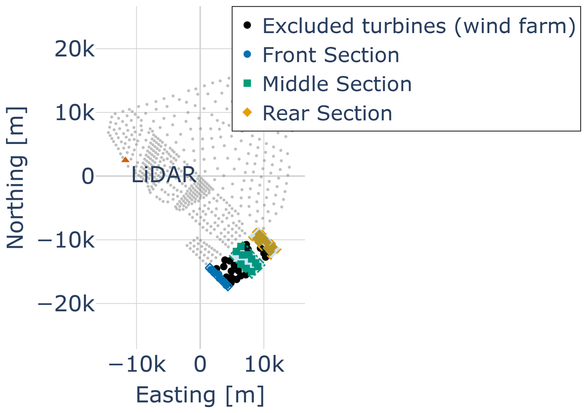
Figure 1 Wind farm layout showing the lidar system and the designated study sections for southwest wind conditions. Black dots represent the wind turbines within the wind farm that were excluded from the study, and light gray dots are other wind farms within the same cluster given for context.

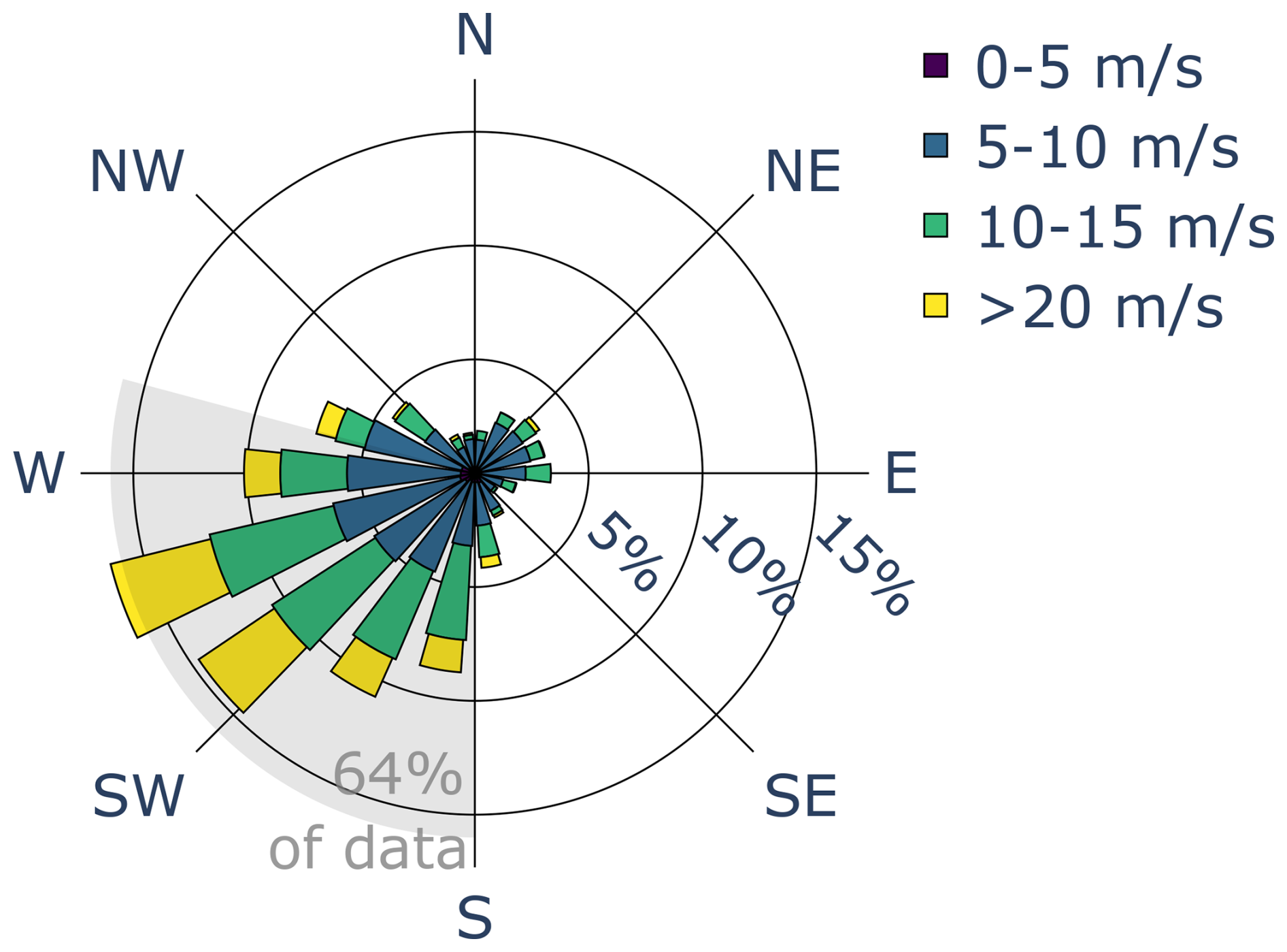
Figure 2 Wind rose illustrating the distribution of wind directions and rotor wind speeds, highlighting the study region where 64 % of the data points are concentrated.

After these filtering steps, the final dataset comprised over 600 000 intervals of 10 min duration, representing approximately 25 % of the raw data for the studied wind sector. The resulting accepted and rejected sets are shown in Fig. 3.

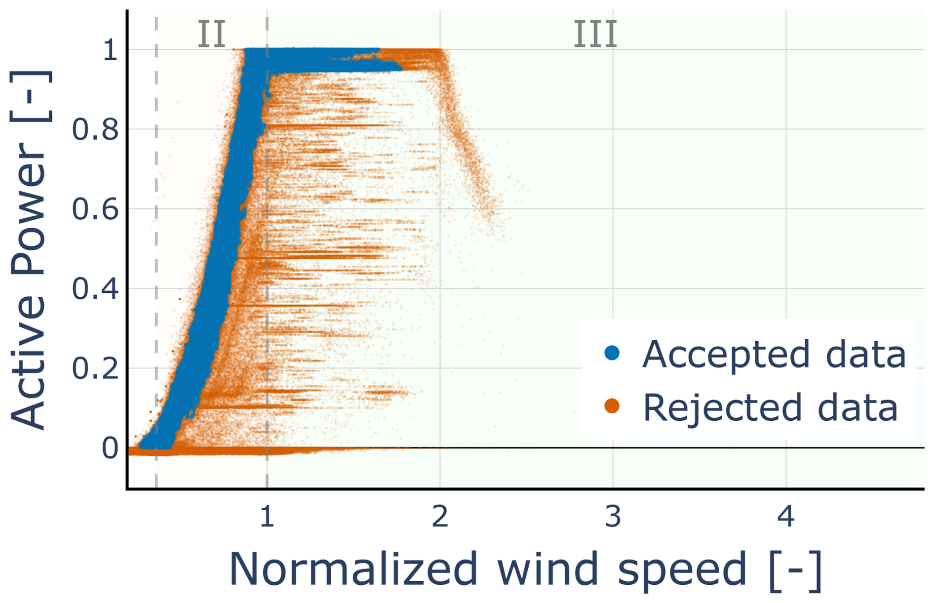
Figure 3 The raw dataset is shown: blue indicates the accepted data used in this study, and orange denotes the rejected data. Region II refers to the torque control region and region III to pitch control.

3 Methodology

This study evaluated the correlation of environmental parameters across different sections of a wind farm. It also assessed the potential application of IEC corrections in SCADA-based performance evaluations within an offshore wind farm, specifically by examining their impact on correlations with power production and the variance of the power curve. To achieve the objectives of the study, after data collection and filtering, the following procedure was followed:

• Section division. The dataset was divided into three sections: the front (first row), the middle (middle section), and the rear (end of the farm).

• Active power deviation (PD). Power production was expressed as the active power deviation from the manufacturer's power curve.

• IEC corrections. The wind speed and the power output were adjusted using the IEC corrections (IEC, 2022) for wind shear, veer, and TI.

• Correlation analysis. Correlation analysis was performed between environmental parameters and PD before and after the IEC corrections for each section. The effect of IEC corrections was then evaluated.

• Variance analysis. The variance of the active power was traced over different wind speeds, both before and after the IEC corrections, for each section. The effect of IEC corrections on the power variability was then evaluated.

These steps are further explained in the following sections of this paper.

3.1 Section division

Free‐flow wind turbines are defined in accordance with the IEC 61400-12-1:2022 (IEC, 2022) standard, which specifies the criteria for an undisturbed region by accounting for the influence of adjacent wind turbines and obstacles. We applied the recommended method to calculate the valid sectors for each wind turbine in the wind farm, selecting those in the first row that met the standards as free-flow turbines. Throughout, we considered these front-row turbines to represent the site’s inflow TI. The middle and rear sections were defined based on the distance to the nearest first-row wind turbine measured along the flow direction. The section widths were defined so as to ensure they contained a volume of data comparable to that from first-row wind turbines, approximately 156 000 10 min intervals per section. Hence, the datasets were balanced and easily comparable. Figure 1 illustrates the segmentation of the wind farm into these three sections. The wind turbines shown in black in Fig. 1 were intentionally omitted to increase the spacing between sections and produce clearer and more interpretable trends.

3.2 Active power deviation (PD)

This study examined whether each environmental parameter contributes positively or negatively to power output at various locations within a wind farm and across different wind speeds. To isolate the influence of these environmental variables while minimizing the effect of variations in wind speed within each bin, the concept of active power deviation (PD) was employed to normalize the active power, as described below:

$$\begin{array}{}\text{(1)}& {\mathrm{PD}}_i=P_{\text{measured},i}-P_{\text{manufacturer},i},\end{array}$$

where P_measured,i refers to the measured power at the ith wind speed bin, and P_{manufacturer,i} refers to the power given by the power curve of the manufacturer at the ith wind speed bin.

3.3 Inflow metrics from nacelle lidar

Upstream inflow shear (α) and veer (β) were derived from the nacelle lidar wind speeds described in Sect. 2. Each lidar wind speed profile was based on two LOSs at six heights, at a range ∼2 rotor diameters upstream. Assuming negligible vertical velocity and mean yaw alignment, horizontal speed U(z) and direction θ(z) at the sampled heights were reconstructed from the symmetric LOS pair and were regressed against $\ln (z/z_{\mathrm{ref}})$; the slopes gave α (dimensionless) and β (reported in ° (100 m)⁻¹). The expanded instrumental uncertainties for 30 min means were small relative to the natural variability (U_α≈0.01 at α=0.3 and U_β≈0.15°/100 m; k=2); see Appendix A for details. We treated these upwind α and β as boundary conditions for the front section, not as invariants within the array; their wake-modified evolution across rows was analyzed by our front/middle/rear methodology.

3.4 IEC corrections

The atmospheric boundary layer in which a wind turbine operates is a dynamic environment. Different inflow conditions are expected to produce varying power outputs at a wind speed. However, collecting sufficient data in a short time frame for every possible inflow condition to create a multi-variable power curve is practically impossible. The IEC standards recommend a combination of corrections to wind speed and active power to reduce the dependency of power output on environmental parameters. One of the goals of this study was to assess the correlation between each environmental parameter and power output across different sections of the wind farm and evaluate the effectiveness of existing IEC corrections in these sections. Ideally, after applying the corrections, the correlation between the environmental parameters and power output should approach zero. This section briefly discusses the corrections applied in this study.

3.4.1 Wind shear and veer correction

For wind turbines with large rotor diameters, variability in wind speed and direction across the rotor can significantly affect power production. This study employed lidar measurements taken upstream near the wind farm to evaluate the shear and veer coefficients of the wind. The derived coefficients enabled estimation of wind speed and direction at different heights based on the average shear and veer profiles.

According to IEC standards (IEC, 2022), the REWS is defined as

$$\begin{array}{}\text{(2)}& v_{\text{rews}}={\left(\sum _{i=\mathrm{1}}^n{\left(v_i\cos \left({\mathit{\varphi }}_i\right)\right)}^{\mathrm{3}}{\displaystyle \frac{A_i}{A}}\right)}^{\mathrm{1}/\mathrm{3}},\end{array}$$

where n is the number of available measurement heights, v_i is the wind speed calculated at height i based on the shear exponent and the hub height wind speed, ϕ_i is the calculated angle difference between the rotor direction and the wind speed at height i based on the measured difference at hub height, A is the rotor-swept area, and A_i is the ith segment area.

To assess the individual contributions of shear and veer to the REWS, we computed the REWS under two separate conditions: one that excludes veer (ϕ=0) and one that excludes shear (u_i=u_{hub height}). The resulting REWS values were then applied to normalize the wind speed according to the IEC standard.

3.4.2 Turbulence intensity (TI) correction

TI can significantly impact the power output of a wind turbine, particularly within a wind farm, where TI tends to increase (Barthelmie et al., 2007), potentially biasing the power curves across different sections. Because wakes increase TI, absolute $\left|\mathit{\rho }\right|$ can be inflated; therefore, we emphasized between-section differences and $\mathrm{\Delta }\left|\mathit{\rho }\right|$ rather than solely absolute magnitudes. This study employed the TI normalization recommended by the IEC to model the effects of 10 min averaging on power output.

A complete discussion of the normalization process is outside the scope of this paper and is well documented in the IEC standard (IEC, 2022); here, we provide an overview for completeness. The first step is to calculate the zero-turbulence power curve. The zero-turbulence power curve represents the theoretical power output of a wind turbine under idealized conditions in which the wind is completely steady. The normalization process adjusts the active power measured during a 10 min interval by first subtracting a simulated average power, calculated using the ideal zero-TI power curve and the measured wind distribution, and then adding a simulated average power, calculated using the ideal zero-TI power curve and a Gaussian wind speed distribution corresponding to the reference TI. Simulated average power in the context of the IEC standard is the expectation of the zero-turbulence curve P₀ under a wind speed distribution centered at the 10 min mean wind speed v_j (where j indexes 10 min records). Following the IEC, wind speed is modeled as Gaussian with mean μ=v_j and standard deviation σ=I v_j for the measured TI I (of record j), and σ=I_ref v_j for the reference TI I_ref. With this definition, the normalization is given by

$$\begin{array}{}\text{(3)}& {\stackrel{\mathrm{‾}}{P}}_{I_{\text{ref}}}\left(v\right)=\stackrel{\mathrm{‾}}{P}\left(v\right)-{\stackrel{\mathrm{‾}}{P}}_{\mathrm{sim},I}\left(v\right)+{\stackrel{\mathrm{‾}}{P}}_{\mathrm{sim},I_{\text{ref}}}\left(v\right),\end{array}$$

where $P_{I_{\text{ref}}}\left(v\right)$ is the normalized power output, $\stackrel{\mathrm{‾}}{P}\left(v\right)$ is the measured mean power, ${\stackrel{\mathrm{‾}}{P}}_{\mathrm{sim},I}\left(v\right)$ is the simulated average power under the observed TI, and ${\stackrel{\mathrm{‾}}{P}}_{\mathrm{sim},I_{\text{ref}}}\left(v\right)$ is the simulated average power under the reference TI.

3.5 Correlation and linear regression slope analysis

The correlation analysis served a dual purpose. First, it clarified the relationship between power production and inflow conditions at different locations within the wind farm. Second, it evaluated the effectiveness of IEC corrections within the wind farm, which lies outside the current scope of the standard. To achieve these objectives, a sliding-window Pearson correlation (SWC) approach was employed. The SWC was computed as follows: (1) all 10 min records were sorted by nacelle wind speed v; (2) a fixed window of width 0.75 m s⁻¹ was defined; (3) within each window, the Pearson correlation between the variable of interest and the PD was computed; (4) this correlation was assigned to the mean v of that window; and (5) the window was slid forward with one-third overlap, and the previous steps were repeated.

The window was advanced by Δu=0.25 m s⁻¹ (one-third of the 0.75 m s⁻¹ width), and only windows with at least N_min=500 records were retained. In practice, retained windows typically contained $N\gtrsim \mathrm{4}\times {\mathrm{10}}^{\mathrm{3}}$ paired 10 min records, so even small correlations had a 95 % significance threshold. This corresponds to a critical value of about $\left|r\right|\gtrsim \mathrm{0.03}$. Mild serial dependence would reduce the effective sample size slightly and raise this threshold but not enough to affect the conclusions.

We analyzed windows whose mean fell in $\mathrm{0.35}\le \widehat{v}\le \mathrm{1.20}$, spanning region II (torque control) and region III (pitch control). Because the control state of a wind turbine depends strongly on wind speed during normal operation, the sliding window was applied along v. Correlations from each window were then plotted against that window’s mean wind speed, which revealed how the relationship between environmental variables and power production shifted across different wind speeds, both before and after the correction.

Similarly to the correlation analysis, we computed, within each window, the slope β(v) of a simple linear regression of the normalized active power deviation (PD_norm) with respect to TI. The normalized active power deviation is defined as

$${\mathrm{PD}}_{\mathrm{norm}}={\displaystyle \frac{\mathrm{PD}}{P_{\mathrm{rated}}}},$$

where PD is given by Eq. (1), and P_rated is the turbine rated power. We normalized PD by P_rated to express slope-based effect sizes on a dimensionless scale, facilitating comparison across wind speed regimes and across turbines or farms. The slope β(v) therefore provided an additional measure to assess the performance of the TI correction. By plotting the slope against the mean wind speed for each window, both before and after the correction, we observed how the sensitivity of PD_norm to TI changed with wind speed. This approach complemented the correlation analysis by evaluating the effectiveness of the correction in reducing the influence of TI on power output.

3.6 Power curve variability analysis

While correlation analysis is useful for examining whether an environmental parameter influences power output before and after a correction, it has its limitations. Applying a correction can sometimes introduce noise that reduces the observed correlation between the environmental parameter and active power, effectively masking the true dependency. This means that relying solely on correlation analysis may not fully capture the impact of the correction. To more effectively assess the effect of a correction, we examined the variability of active power at different wind speeds across various sections of the wind farm, both before and after the correction. Specifically, we used the median absolute deviation (MAD), as shown in Eq. (4). This approach allowed us to identify how the corrections affected the variance of the power curve. Moreover, MAD is less sensitive to outliers, making it a robust measure for this analysis:

$$\begin{array}{}\text{(4)}& {\text{MAD}}_{P_j}=\text{median}\left(\left|P_{j,i}-\text{median}\left(P_j\right)\right|\right),\end{array}$$

where P_j,i is the active power measurement i at wind speed bin j, and median(P_j) is the median of all active power measurements at wind speed bin j.

In interpreting the results, the sliding-window Pearson correlations were therefore used primarily to identify the sign and relative pattern of the dependence across wind speed and between sections (front, middle, rear), while the regression slopes and MAD-based variability metrics were used to quantify the associated effect sizes in terms of changes in power and PD.

4 Results and discussion

This section analyzes the influence of environmental parameters – wind shear, veer, and TI – on power production in different sections of the wind farm, both before and after applying IEC corrections. Three main types of plots are utilized: (1) Pearson correlation plots that show the relationship between each environmental parameter and PD across wind speed windows; (2) corresponding Pearson correlation plots for the corrected values, which allow for an assessment of the effectiveness of the corrections; and (3) for TI, additional linear regression slope plots that evaluate the sensitivity of normalized active power deviation to TI before and after the correction. In the correlation plots, the markers are shown only when the correlation is statistically significant (95 % confidence).

In interpreting the correlation results, it is important to recognize that pairwise Pearson coefficients are expected to be modest in operational data because multiple inflow parameters (wind speed, TI, shear/veer, stability), wake interactions, and active control jointly govern turbine response. Our correlations target secondary inflow descriptors (TI, shear, veer) rather than the primary driver (wind speed), so small $\left|\mathit{\rho }\right|$ values are not only expected but consistent with offshore field evidence (peak values ∼0.16–0.21) (Seifert et al., 2021). Low $\left|\mathit{\rho }\right|$ does not imply irrelevance: when conditioned appropriately, shear and veer still produce statistically significant shifts in performance (e.g., REWS-based segregation yielding departures of up to ∼5 % for a 1.5 MW turbine) (Murphy et al., 2020). We therefore emphasize the structure of the correlation profiles, sign changes across wind speed bands, regime dependence (torque-to-pitch transition), front–middle–rear contrasts, and pre-/post-correction trends, rather than the absolute magnitudes alone. Accordingly, we use the sliding-window correlations primarily to identify these sign and regime patterns in the correlations between inflow descriptors and PD, whereas effect magnitudes are characterized using regression slopes based on PD_norm and within-bin active power variability (MAD).

A related caveat is farm-scale blockage, which manifests primarily as a quasi-uniform reduction in upstream wind speed on several rotor diameters – measured at ∼3.4 % at 2D and ∼1.9 % at 7–10D in onshore field campaigns (Bleeg et al., 2018) and observed offshore with lidar scanning such as ≲2 %, extending tens of rotor diameters upstream (Schneemann et al., 2021). In this study, we do not attempt to reconstruct an undisturbed far-upstream free-stream. Instead, all analyses are conditioned on the measured nacelle wind speed v and on the inflow descriptors (TI, shear, veer) in the selected upwind sector, and we interpret the results as conditional relationships between turbine-level PD and these local inflow parameters. From this rotor-centric point of view, a nearly uniform reduction in upstream wind speed acts mainly as a common shift in the wind speed distribution and is not expected to change the conditional dependence of PD on shear, veer, or TI within a given wind speed bin, nor the front–middle–rear contrasts that we report. Farm-scale blockage may, in principle, induce small systematic changes in the inflow profile itself; we therefore discuss it as a limitation of the present dataset and note that a dedicated, quantitative blockage assessment would be required to refine absolute power levels and AEP estimates, which lies beyond the scope of this performance-characterization study.

4.1 Wind shear and veer correction

Figures 4 and 5 illustrate the correlation of wind shear with PD before and after applying the REWS (shear-only) correction. A key observation is that the correlation patterns between wind shear and power production change depending on the position within the wind farm. Specifically, the influence of the upwind wind shear is most pronounced in the front section, with its influence weakening further downstream. Negative correlations are observed in the front row, while positive correlations appear in the rear section. This shift may be explained by changes in the upwind wind profile as it moves through the farm, where wind turbine wakes enhance mixing and alter the shear and veer characteristics; however further investigation is required to understand the mechanism. Across these correlation profiles, the absolute values of the Pearson coefficients remain modest ($\left|\mathit{\rho }\right|\lesssim \mathrm{0.3}$), as expected for secondary inflow descriptors in operational data.

Figure 5 shows that even though the REWS correction is applied based on the time-averaged inflow profile, it reduces the correlation with the wind shear on the front section, while it increases the apparent coupling in the middle and rear sections. In our case, based on the available measurements, the average correction is approx. 0.1 m s⁻¹, with a standard deviation of 0.08 m s⁻¹.

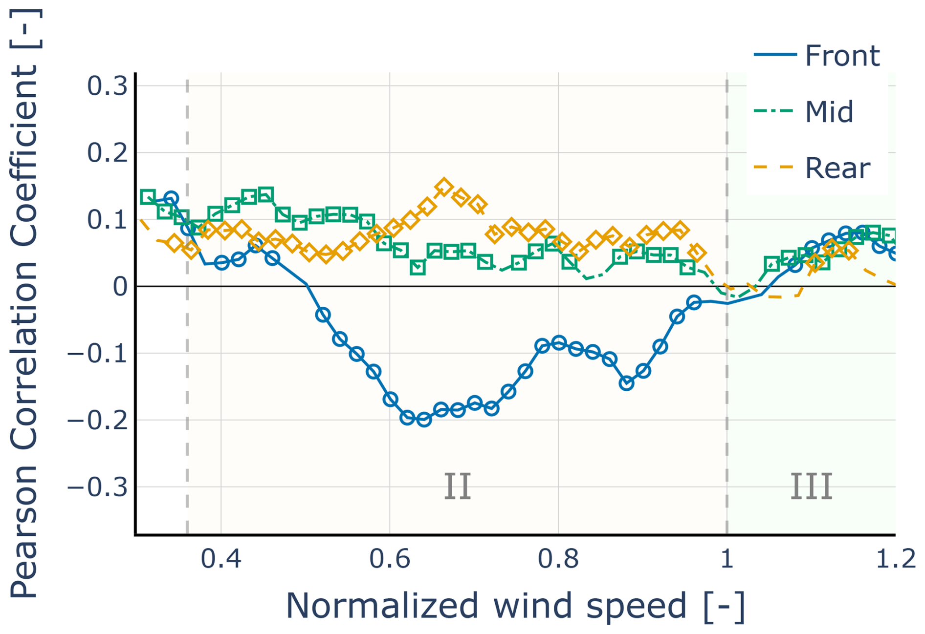
Figure 4 Sliding-window correlation between wind shear α and active power deviation PD before REWS; markers shown only if p<0.05.

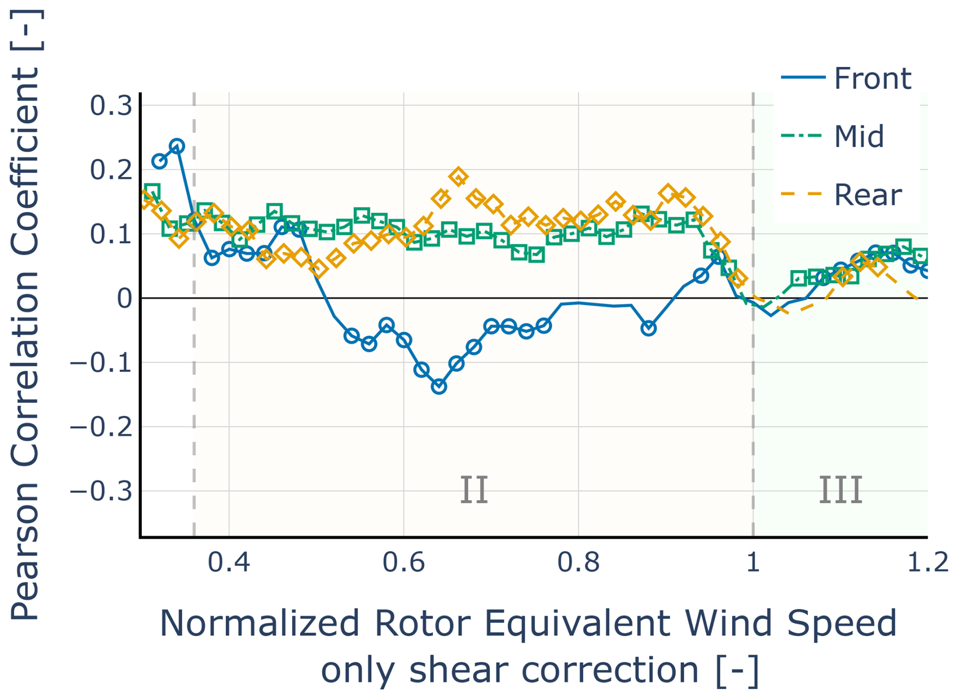
Figure 5 Sliding-window correlation between wind shear α and active power deviation PD after REWS (shear-only) correction; changes across the normalized REWS indicate where coupling is reduced or enhanced.

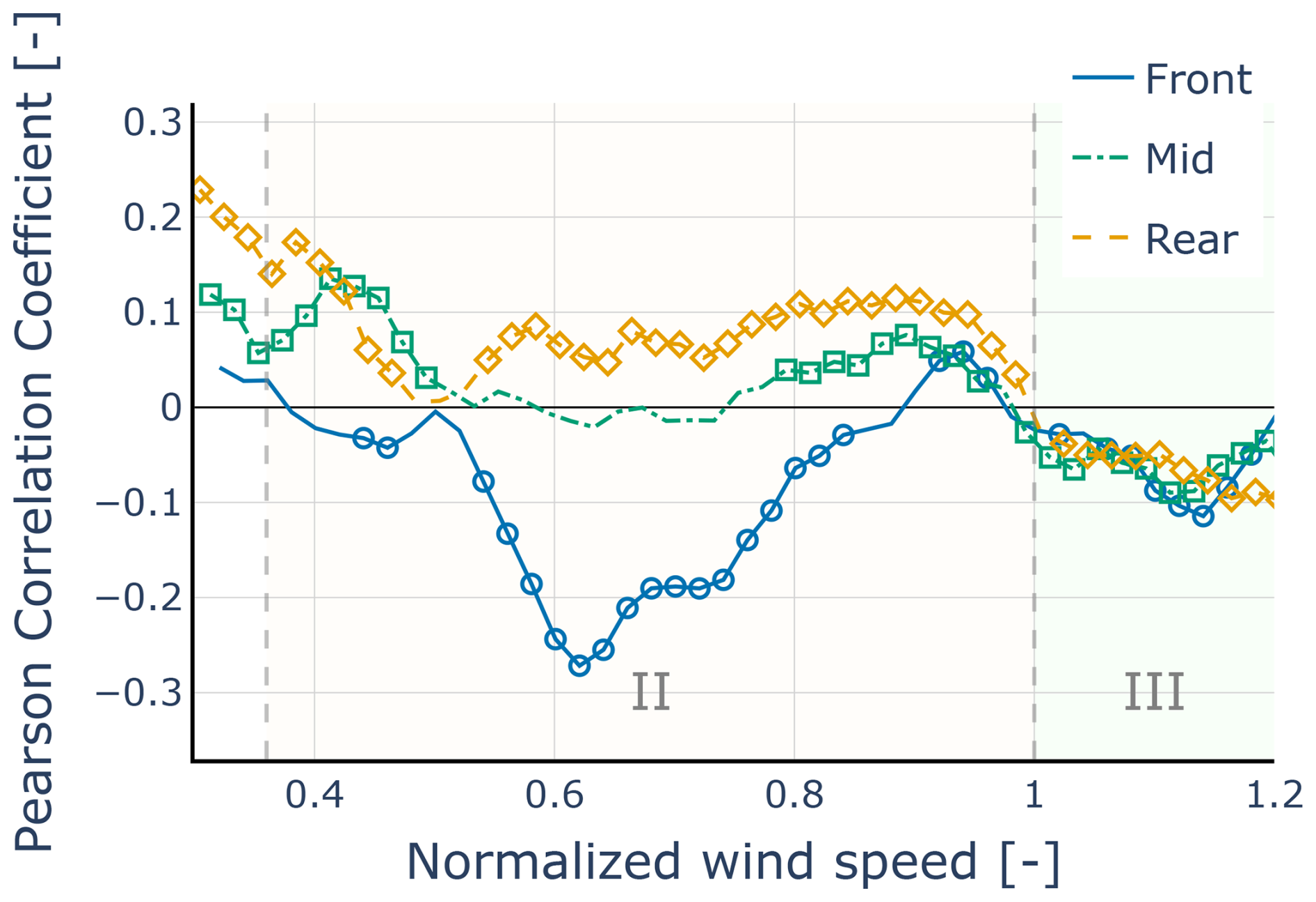
Figure 6 Sliding-window correlation between wind veer β and active power deviation PD before REWS; markers shown only if p<0.05.

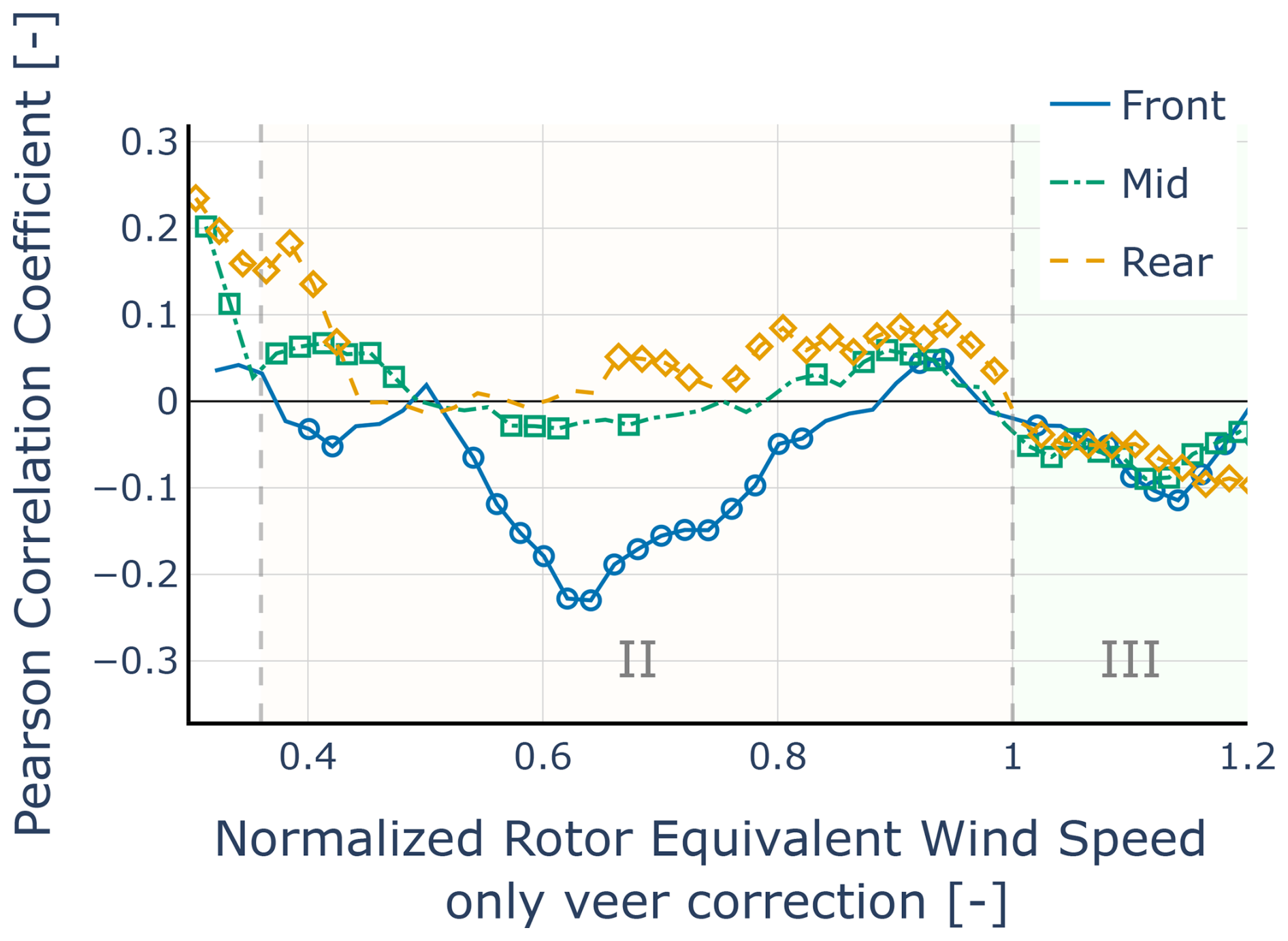
Figure 7 Sliding-window correlation between wind veer β and active power deviation PD after REWS (veer-only) correction; changes across the normalized REWS indicate where coupling is reduced or enhanced.

Although the distance to measure wind shear and veer is relatively short for an offshore setting, obtaining more precise data closer to the wind farm – without assuming a wind shear profile based on power law (Debnath et al., 2021) – may improve the correction. Another possible explanation is that shear and veer are correlated with other factors, such as TI, which also affect power output. This interdependence makes it challenging to correct using REWS alone.

The full veer–power correlation profiles before applying any correction and after applying the REWS (veer-only) correction are shown in Figs. 6 and 7, respectively. The correlation patterns between wind veer and power output change depending on the position within the wind farm. In the front section, wind veer is negatively correlated with turbine power output, while positive correlations are observed in the rear section. Given that veer is linked with shear as described by Kelly and van der Laan (2023), our results suggest that both parameters exert a similar spatially dependent correlation with turbine performance. The REWS correction has a small impact on the effect of wind veer in the front section but does not decouple the correlation of inflow of upwind wind veer from the power output of the wind turbine. This could be a result of the small correction that the REWS applies to the wind speed as suggested by (Van Sark et al., 2019). It is important to note that the REWS correction is primarily designed to adjust for variations in the energy flux over the rotor due to wind shear and veer. However, the wind profile can also affect the aerodynamic load on the turbine blades. Consequently, even after applying the REWS correction, the residual correlation between wind veer or shear and power output indicates that these effects may not be fully mitigated.

4.2 TI correction

Figures 8 and 9 compare the correlation between TI and wind turbine power output before and after applying the IEC-based correction at different locations within the wind farm. Additionally, Figs. 10 and 11 illustrate the sensitivity of the normalized active power deviation to TI by presenting the slope β of the linear regression between TI and normalized PD. These slopes were computed over the same 0.75 m s⁻¹ windows with a 0.25 m s⁻¹ stride, with typical window sizes exceeding 4×10³ paired records. In Fig. 8, the correlation of TI at various wind speeds aligns with the expected behavior based on theoretical modeling (Saint-Drenan et al., 2020). Specifically, as expected by the literature, the front section has a positive correlation for normalized wind speeds 0.36–0.84 and a negative correlation at higher wind speeds. However, the rear sections have significantly different behavior for normalized wind speeds of up to 0.84. Although the negative correlations are initially small at wind speeds below 0.7, they become considerably stronger as the wind speeds approach the rated value. All sections have similar behavior at normalized wind speeds greater than 0.84; however, there are significant differences at lower wind speeds. Although all sections exhibit similar behavior at normalized wind speeds greater than 0.84, the significant differences at lower wind speeds suggest that the turbulent characteristics in the front-row region are significantly different from those in the waked region.

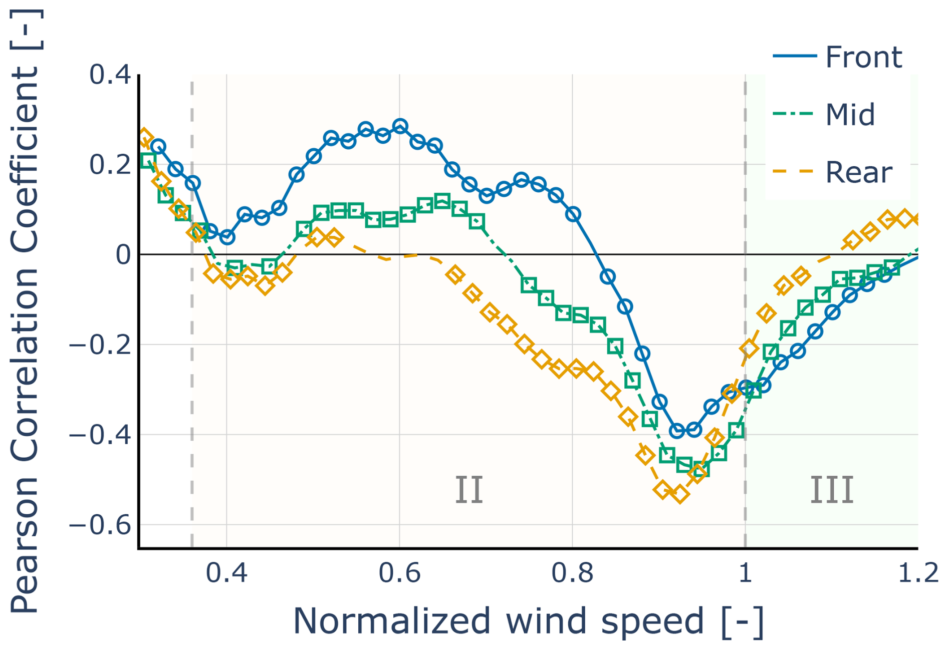
Figure 8 Sliding-window correlation between TI and active power deviation PD before TI normalization; markers shown only if p<0.05.

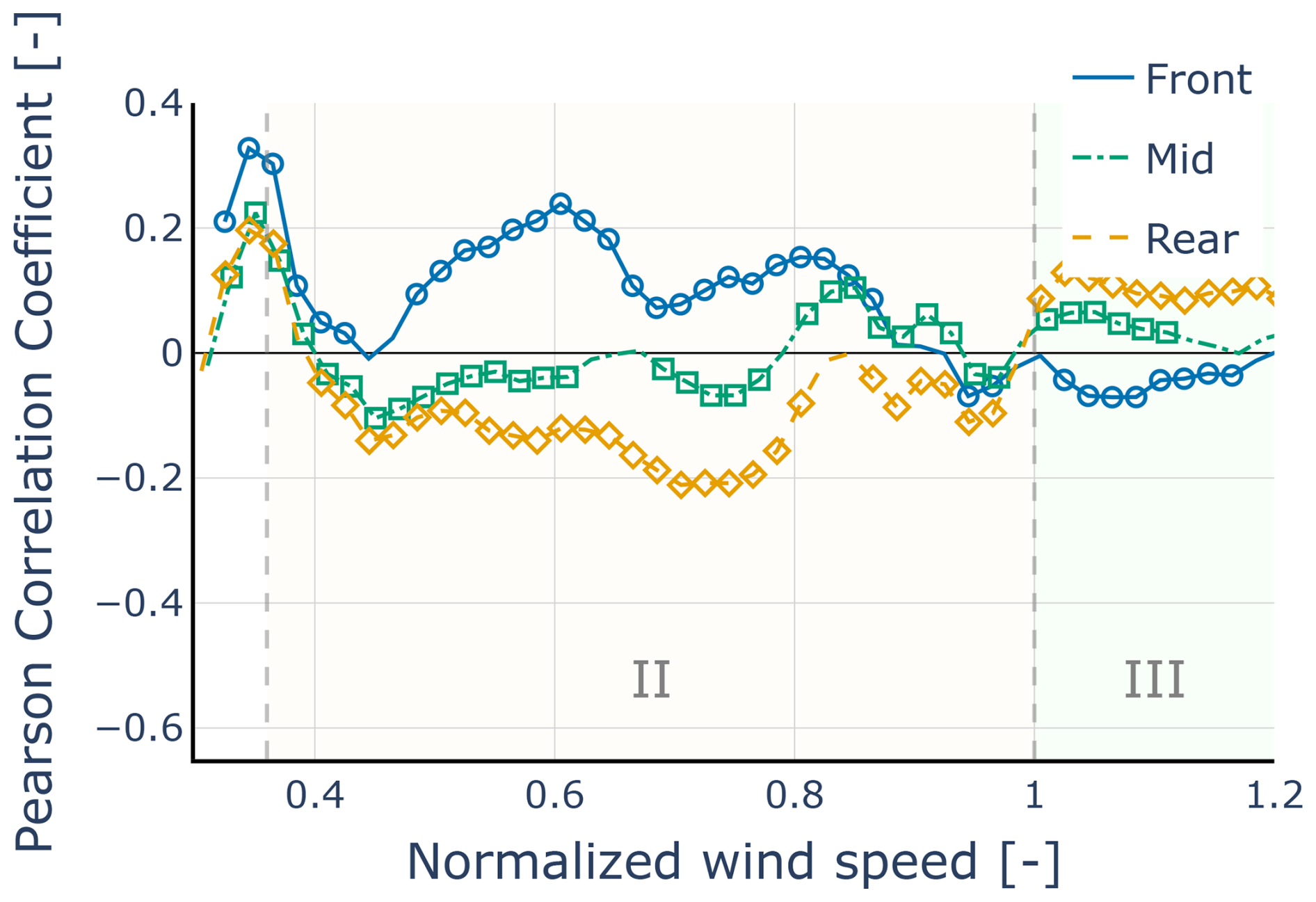
Figure 9 Sliding-window correlation between TI and active power deviation PD, after TI normalization; changes across the normalized wind speed indicate where coupling is reduced or enhanced.

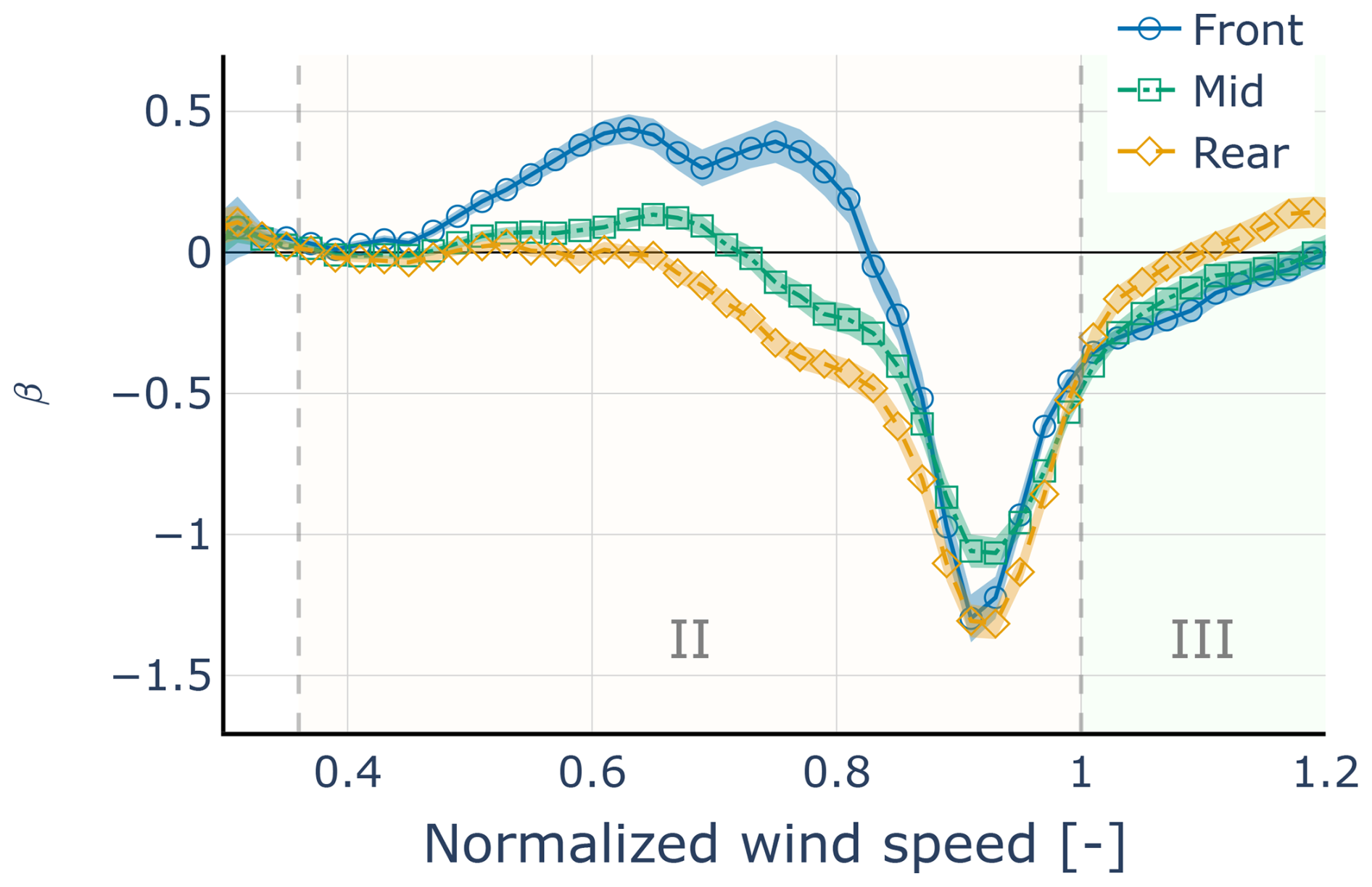
Figure 10 Linear regression slope between TI and normalized active power deviation at various wind speeds before applying the TI normalization.

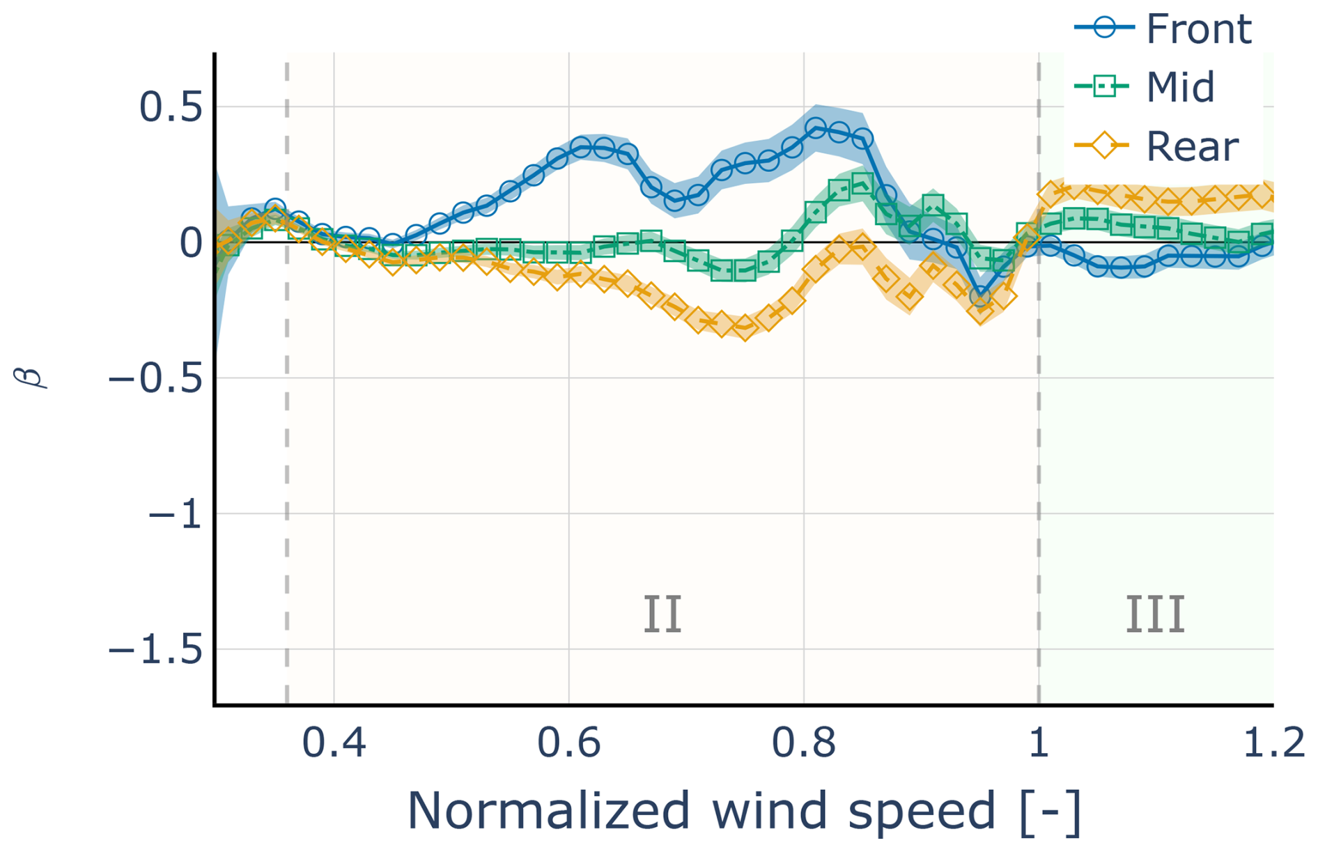
Figure 11 Linear regression slope between TI and normalized active power deviation at various wind speeds after applying the TI normalization.

The slope analysis presented in Fig. 10 complements the correlation findings by quantifying the sensitivity of PD to TI. The slopes β indicate how much the PD changes with a unit change in TI. The front section shows a small positive slope in the normalized wind speed range of 0.4 to 0.65, indicating a positive effect of TI on power. In contrast, in the same wind speed ranges, the middle and rear sections show lower slopes, indicating that these sections of the wind farm have a lower sensitivity to TI compared to the front section at low wind speeds. However, for normalized wind speeds above 0.84, all sections show a higher sensitivity to TI.

The results of the IEC correction in Fig. 9 indicate that, in the front and middle sections, the IEC correction reduces the correlation by about half for normalized wind speeds between 0.4 and 0.6 and further decreases TI dependency for wind speeds greater than 0.8. However, the correction behaves differently in the rear sections, where it overcompensates for TI effects and even shifts the correlation to the negative side for a wind speed lower than 0.6. For normalized wind speeds above 0.84, the correction appears to eliminate most of the TI dependency.

Similarly, the slope analysis in Fig. 11 shows that the sensitivity of PD to TI is significantly reduced after the correction in all sections for high wind speeds. For low wind speeds in the rear section, the slopes become more negative or remain low, indicating that the correction may be overcompensating or not adequately accounting for wake-induced turbulence effects. The overcompensation observed in the rear sections may be due to the increased wake-induced turbulence, which might differ significantly from the inflow turbulence conditions assumed in the IEC correction methodology.

This suggests that the IEC TI correction may not be fully applicable within the wake-affected regions of the wind farm. However, it can still significantly correct for a large part of the TI effect on power production.

4.3 Effect on the variability of the power curve

To further examine how turbine location affects power production, we quantified the variability of active power in each section using the MAD. First, we established a baseline for each section (Fig. 12) representing the variability before any corrections. In contrast, the rear section exhibits less variability than the front section, despite the presence of wakes and increased turbulence inside the wind farm.

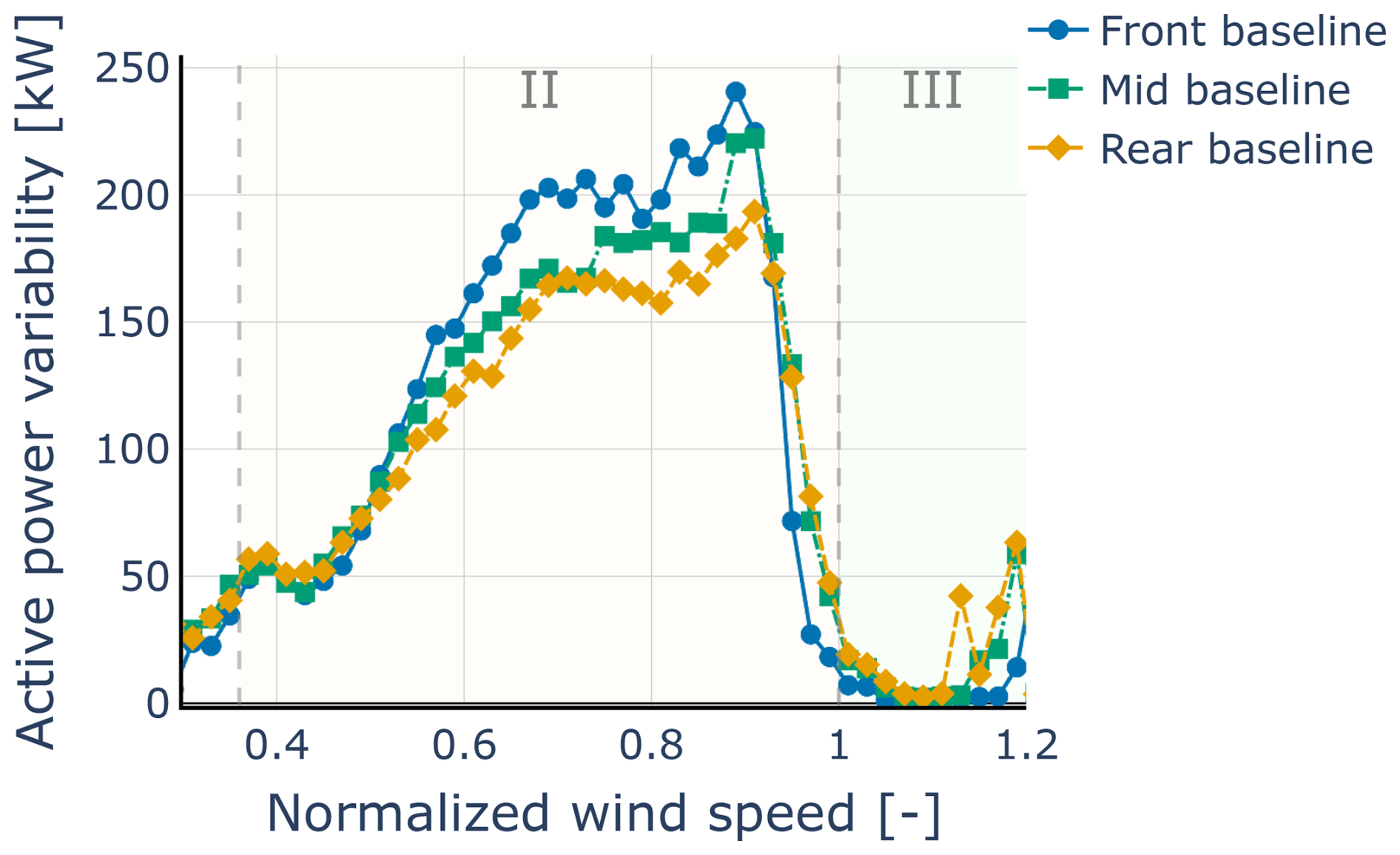
Figure 12 MAD of active power output across different wind speed bins for the different sections of the wind farm. The baseline curve represents the power curve MAD without any corrections.

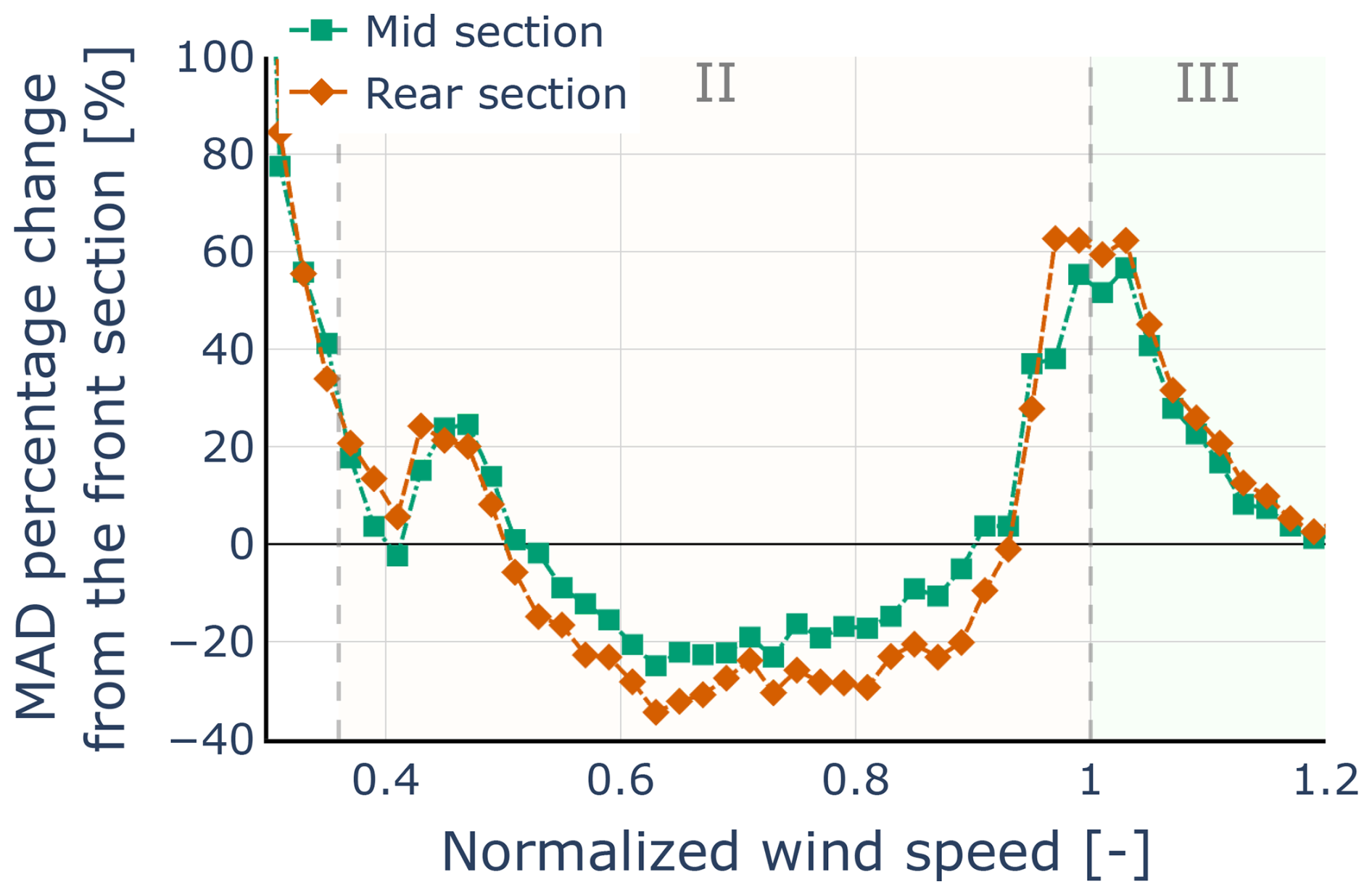
Figure 13 Percentage change in the MAD of active power output for the middle and rear sections compared to the front section.

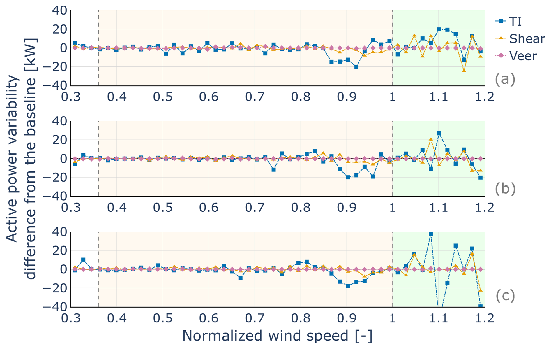
Figure 14 Differences in the MAD of active power output after each correction from the baseline across different wind speed bins. (a) Differences in the front section, (b) in the middle section, and (c) in the rear section of the wind farm.

For clarity, Fig. 13 shows the percentage change in MAD between the middle and rear sections compared to the front section. Both sections show reduced active power variability for normalized wind speeds between 0.64 and 0.92, with the rear section showing reductions of more than 30 %. Next, we evaluated how the applied corrections influence this variability. Figure 14 illustrates the changes in MAD after each correction for each section. Overall, the corrections result in relatively small changes in MAD, with the only significant reduction in active power variability occurring from the TI correction for below-rated conditions.

4.4 Evaluation of correction-induced correlation changes

To visualize how each correction affects the correlation between environmental factors and power output, Figs. 15, 16, and 17 present the absolute change in correlation in the front, middle, and rear sections of the wind farm. The metric shown is the absolute-correlation shift $\mathrm{\Delta }\left|\mathit{\rho }\right|\equiv \left|{\mathit{\rho }}_{\text{corrected}}\right|-\left|{\mathit{\rho }}_{\text{uncorrected}}\right|$, where ρ is the Pearson correlation coefficient, as a function of wind speed, with different lines representing the corrections for wind shear, veer, and TI. Negative $\mathrm{\Delta }\left|\mathit{\rho }\right|$ means the correction reduced the apparent coupling; positive means it increased.

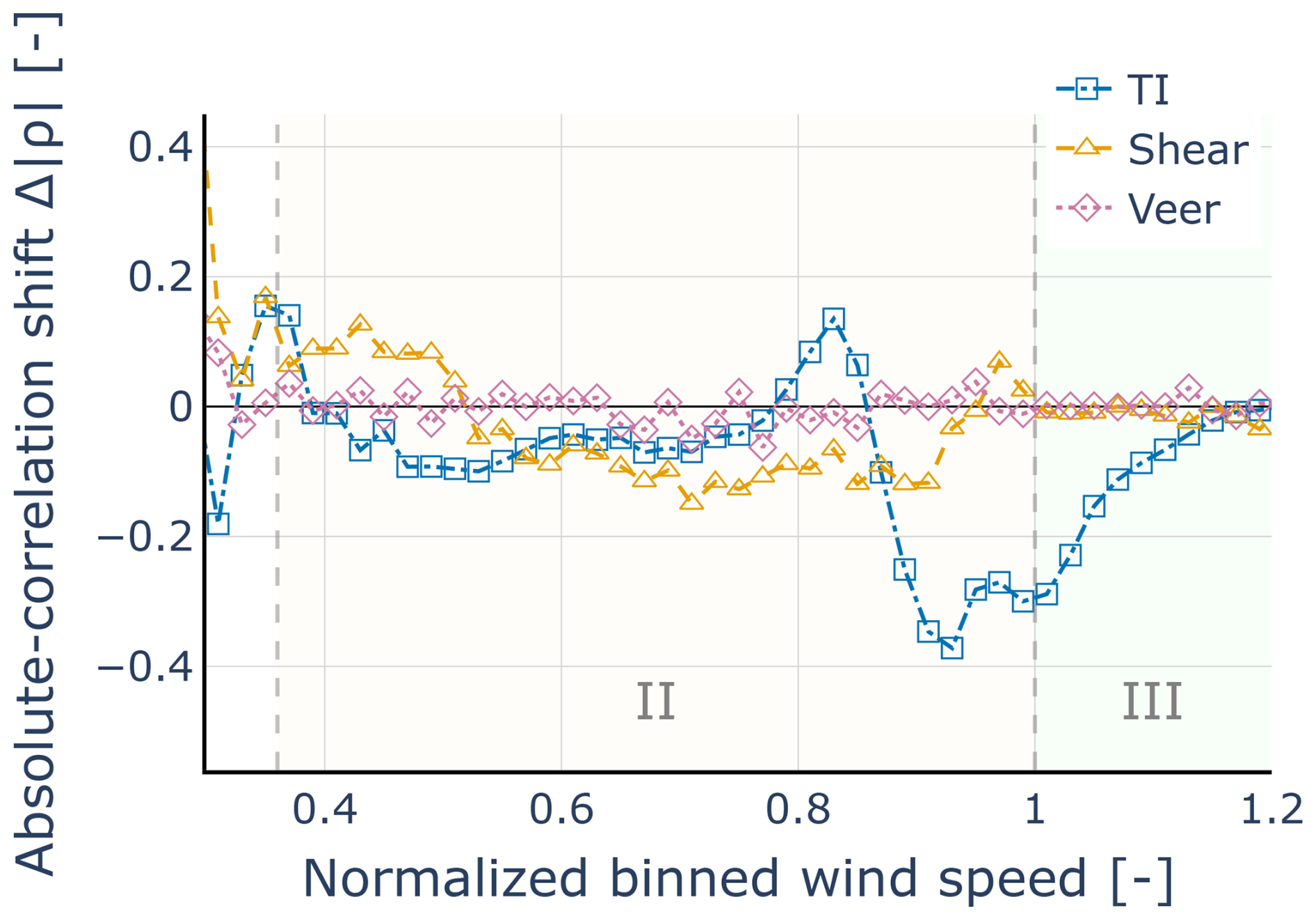
Figure 15 Front section: change in correlation magnitude relative to the uncorrected baseline, $\mathrm{\Delta }\left|\mathit{\rho }\right|$, versus wind speed.

Figure 16 Middle section: change in correlation magnitude relative to the uncorrected baseline, $\mathrm{\Delta }\left|\mathit{\rho }\right|$, versus wind speed.

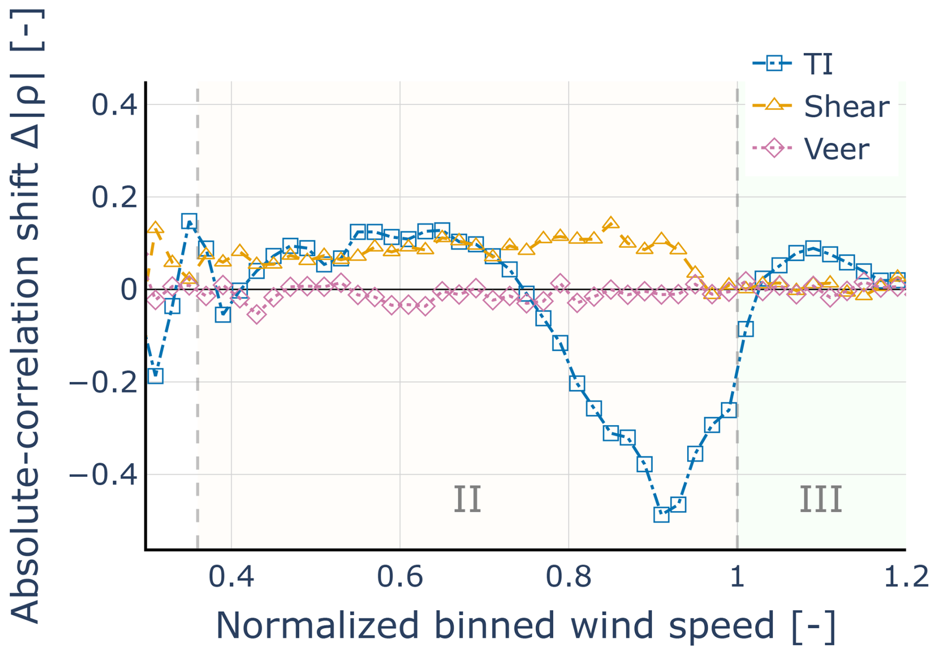
Figure 17 Rear section: change in correlation magnitude relative to the uncorrected baseline, $\mathrm{\Delta }\left|\mathit{\rho }\right|$, versus wind speed.

As shown in these figures, the REWS corrections for wind shear and veer offer a small reduction in the correlation for the front section for wind speeds above $v/v_{\text{rated}}\approx \mathrm{0.6}$ (Fig. 15). However, for lower wind speeds, the corrections increase the coupling (Fig. 15). In the middle and rear sections, these corrections slightly increase the correlation (Figs. 16 and 17). In comparison, the effect of the TI correction is stronger. The TI correction has a smaller effect in the front section (Fig. 15) but becomes more significant in the middle and rear sections, particularly as wind speeds approach the rated value, while the picture is less clear for lower wind speeds (Figs. 15, 16, and 17).

5 Conclusions

This study was carried out to provide a detailed empirical assessment of how inflow conditions and turbine location impact power production and the effectiveness of IEC corrections in a large offshore wind farm. Using 13 months of 10 min SCADA and the upstream nacelle lidar profiles, we asked how vertical shear, directional veer, and TI couple to power across the front, middle, and rear sections of a large offshore wind farm and how IEC 61400-12-1:2022 normalizations perform in these regimes. We find that inflow–power coupling is strongly location dependent, IEC-style normalizations reduce apparent coupling mainly near free-stream conditions, and TI inside the wind farm behaves differently from free-stream TI below rated wind speed.

The influence of wind shear and veer revealed a distinct spatial dependency. In the front row (free-stream), shear and veer correlate negatively with power, while in middle and rear rows, the correlation is positive. This sign flip is consistent with wake-induced mixing that flattens vertical gradients and changes the effective inflow seen by downstream rotors. The REWS normalization has a limited practical effect: it reduces coupling slightly in the front section but does not decouple shear/veer from power inside the farm and can even increase coupling downstream.

A similarly complex, location-dependent behavior was observed for TI. It shows the expected positive correlation with power at sub-rated wind speeds in front/middle sections and becomes negative near rated; in the rear section, TI is already negatively correlated at lower normalized speeds, indicating that wake-induced TI differs from free-stream TI. The IEC TI correction performs well for wind speeds above $v/v_{\mathrm{rated}}\gtrsim \mathrm{0.8}$ across all sections and reduces sub-rated TI coupling in the front/middle sections. However, in the rear section at low speeds, the correction tends to overcompensate, as seen in Fig. 17.

The analysis of power production variability showed that the median absolute deviation (MAD) within wind speed bins is lower in middle and rear rows than in the front row, implying more stable downstream power inside the wake at a given wind speed. Corrections have small effects on MAD overall; only the TI correction yields a noticeable reduction below rated wind speed.

These results highlight that inside wind farms, the inflow differs significantly from free-stream assumptions. While current IEC normalizations (REWS, TI) are useful near free-stream conditions, they can be insufficient or regime dependent in waked rows. Adding inflow descriptors beyond standard IEC parameters, e.g., turbulent kinetic energy (TKE) (Kumer et al., 2016), could improve power performance evaluations and reduce uncertainty for large offshore projects.

Finally, while these findings are robust, it is important to note the study's context. Pairwise correlations are inherently modest in operational data, and the lidar was located offsite, which we screened and treated conservatively; these constraints likely make our reported couplings conservative rather than inflated. Overall, location-dependent inflow effects and regime-dependent normalization performance argue for farm-aware evaluation methods that extend beyond free-stream IEC assumptions when assessing turbines inside wakes.

Appendix A: Nacelle lidar reconstruction and uncertainty

Methodology

The horizontal wind vector is reconstructed from the lidar's line-of-sight (LOS) measurements using a two-beam de-projection method. At each measurement height, this technique uses two quasi-simultaneous beams at symmetric azimuth angles ($\pm a=\pm \mathrm{15}\mathit{°}$) to solve for the horizontal wind components (u_i,v_i). This reconstruction relies on the following assumptions: (i) negligible vertical wind velocity (w≈0), (ii) mean yaw alignment of the nacelle with the incoming flow, and (iii) horizontal homogeneity of the wind field across the narrow probed sector (Letizia et al., 2023).

Continuous-wave (CW) lidars, like the one used in this study, measure a range-weighted average of the LOS velocity over a probe volume that increases with distance. This spatial averaging, combined with the geometric limitations of LOS measurements, can smooth turbulence and introduce biases if not properly accounted for. Our reconstruction and subsequent averaging can mitigate these effects. While absolute TI may be attenuated, the structure of the results we interpret (e.g., sign changes with wind speed, front–middle–rear contrasts, and $\mathrm{\Delta }\left|\mathit{\rho }\right|$ trends) is not expected to be sensitive to a nearly uniform attenuation of fluctuations. We nevertheless acknowledge residual bias as a limitation.

Shear, veer, and uncertainty estimation

From the reconstructed wind vectors at each height, the vertical wind shear exponent (α) is estimated by fitting the wind speeds to a power-law profile, while the wind veer (β) is estimated from the slope of a linear fit to the wind direction profile, θ(z). The final veer is reported in degrees per 100 m (° (100 m)⁻¹).

Uncertainties are propagated from the instrument's LOS noise (σ_v=0.10 m s⁻¹, as specified by the manufacturer) to the reconstructed wind speed and direction at each height. These propagated variances are then used as weights in a weighted least squares (WLS) fit for the shear and veer parameters. The covariance matrix from the WLS solution provides the standard uncertainty for α and β for each instantaneous scan. For our measurement geometry (measurement plane distance from the optical head R=420 m), the expanded uncertainties per scan for the shear and veer estimations on average are

$$U_{\mathit{\alpha }}\approx \mathrm{0.06}\text{and}{U}_{\mathit{\beta }}\approx \mathrm{0.86}\mathit{°}/\mathrm{100}\mathrm{m}(k=\mathrm{2}).$$

Uncertainty in 30 min averages

The final operational estimates are 30 min means. While the lidar samples at 1 Hz, we assume the period for an effective independent measurement is 1 min to account for autocorrelation in the high-frequency data. This results in an effective number of independent samples, n_eff=30, within each 30 min average. The standard uncertainty in the 30 min mean is found by scaling the uncertainty in a single 1 min estimate by $\mathrm{1}/\sqrt{n_{\mathrm{eff}}}$, which yields the final expanded uncertainties reported in the main text:

$$U_{\mathit{\alpha }}\approx \mathrm{0.01}{U}_{\mathit{\beta }}\approx \mathrm{0.15}\mathit{°}/\mathrm{100}\mathrm{m}(k=\mathrm{2}).$$

Appendix B: NORA3-based representativeness assessment

Dataset and rationale

To test whether the upstream nacelle lidar measurements are representative of the inflow in the wind farm front section, we used the NORA3 dataset as an independent external reference. NORA3 is the regional atmospheric reanalysis of MET Norway that provides gridded hourly wind fields over the North Sea (Haakenstad et al., 2021; Haakenstad and Breivik, 2022). Here, NORA3 is used to assess spatial homogeneity between the lidar location and the farm and to define conservative thresholds for extreme shear and veer. No NORA3 variables enter the correlation or correction analyses.

Homogeneity assessment and filtering

For each hour, we derive vertical shear (α) and veer (β) from NORA3 at two points: (i) the nearest lidar grid cell and (ii) the closest cell of the front section of the farm. The separation of these points is ≈23.5 km. Shear α is estimated by a power-law fit of U(z) across the available levels; veer is the linear slope of the unwrapped direction with height, reported as β₁₀₀=100 β in ° (100 m)⁻¹. This yields paired hourly series {α_L(t),α_F(t)} and {β_L(t),β_F(t)}, where subscripts L and F denote the lidar-proximal grid cell and the farm’s front-section grid cell, respectively.

We compare the two locations using quantile–quantile (Q–Q) plots and coincident hour time series. As shown in Fig. B1a and b, the Q–Q plots for both shear and veer show strong agreement between the two locations through the core of the distributions, with some expected divergence in the extreme tails. The time series (Fig. B2a and b) further confirm that the two sites track each other well.

This strong agreement validates the general representativeness of the lidar measurements. We therefore apply a conservative central 95 % filter directly to the lidar-derived distributions of shear and veer, excluding the extreme tails where the NORA3 analysis indicates a higher potential for inhomogeneity. As specified in the main text, we keep the intervals as

$$\mathit{\alpha }\in [\mathrm{-}\mathrm{0.05},\mathrm{0.21}],{\mathit{\beta }}_{\mathrm{100}}\in [-\mathrm{3},\mathrm{21}]\mathit{°}/\mathrm{100}\mathrm{m},$$

which are used as fixed limits in the study.

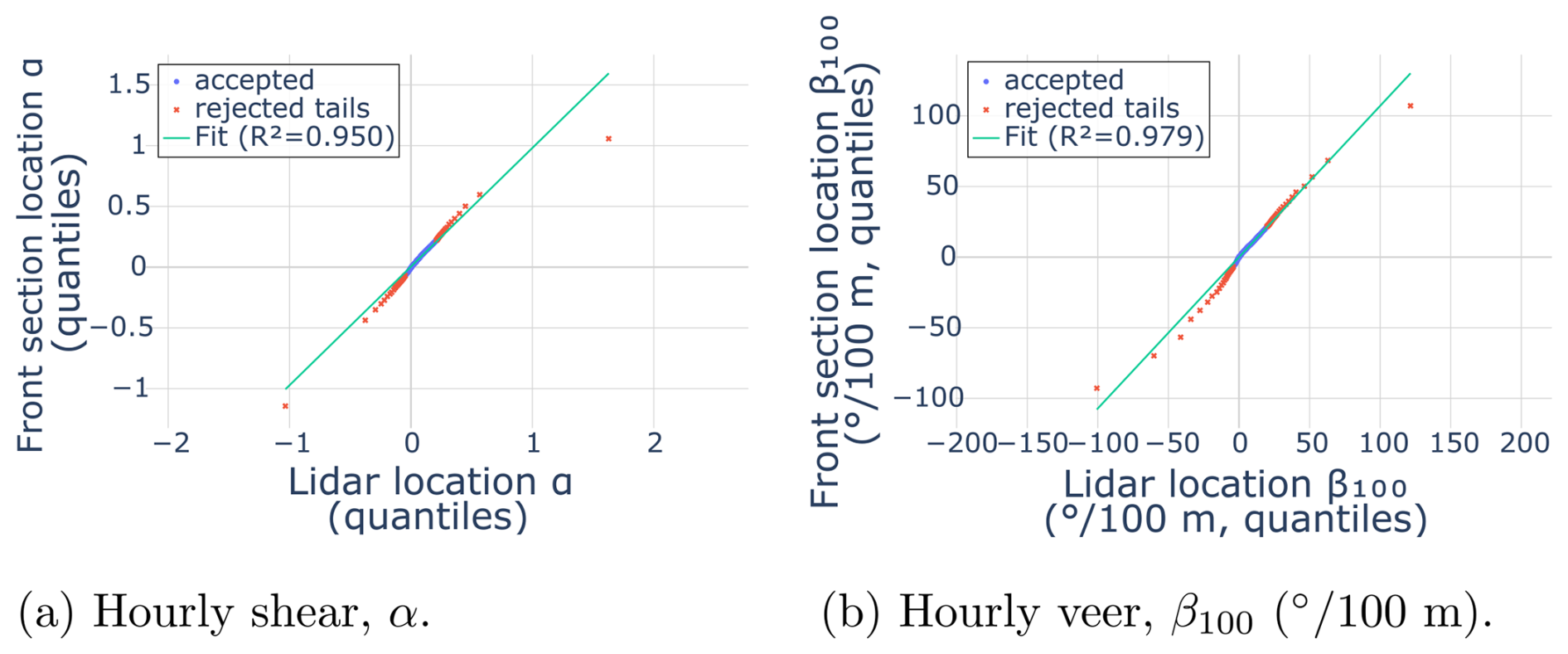
Figure B1 Q–Q comparisons between the lidar-nearest and front-of-farm NORA3 grid cells: (a) hourly shear, α, and (b) hourly veer, β₁₀₀ (° (100 m)⁻¹). In both panels, the lidar-nearest grid cell is shown on the x axis and the front-of-farm grid cell on the y axis. The solid lines denote ordinary least-squares fits, with R²=0.95 for shear and R²=0.979 for veer.

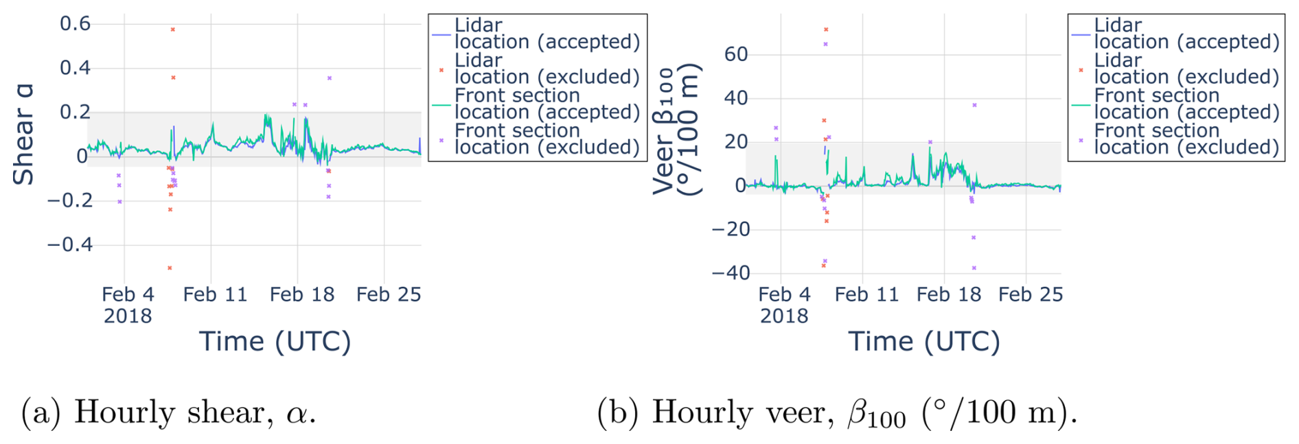
Figure B2 Hourly shear and veer at the lidar-nearest and front-of-farm NORA3 grid cells: (a) shear, α, and (b) veer, β₁₀₀ (° (100 m)⁻¹). Accepted and excluded values are shown separately. The retained central 95 % limits applied to the lidar data are $\mathit{\alpha }\in [-\mathrm{0.05},\mathrm{0.21}]$ and ${\mathit{\beta }}_{\mathrm{100}}\in [-\mathrm{3},\mathrm{21}]$ ° (100 m)⁻¹.

Appendix C: Robustness check of directional sector width

This appendix evaluates the robustness of the main correlation-based findings to the chosen wind direction sector width. The main analysis uses the broad inflow sector 180°–285° (width 105°), selected to preserve robust sample counts per wind speed window and to avoid over-interpreting narrow-direction subsets while preserving stable statistics in each wind speed window. To assess whether the main conclusions depend on the sector definition, we repeat the full correlation workflow using a narrower directional filter.

Method

We define a 30° sub-sector around the midpoint of the main sector, spanning [217.5°, 247.5°]. All other filtering steps (availability criteria, operational filters, HDBSCAN cleaning, lidar advection, etc.) are identical to the main analysis. We then recompute the sliding-window Pearson correlations described in Sect. 3.5, using the same window width (0.75 m s⁻¹), stride (0.25 m s⁻¹), and minimum per-window sample count (N_min=500). The resulting profiles are compared qualitatively to the corresponding wide-sector profiles in Sect. 4, focusing on (i) the sign of the dependence, (ii) the front/middle/rear contrasts, and (iii) the response to the IEC normalizations (REWS and TI correction).

Results

Figures C1–C3 show the narrow-sector correlation profiles for shear, veer, and TI (before and after applying the corresponding IEC corrections). Restricting the sector to 30° reduces the number of samples, yielding slightly noisier correlation trajectories. However, the principal behaviors reported in Sect. 4 are preserved.

For shear and veer (Figs. C1 and C2), the narrow-sector analysis reproduces the main section-wise structure: negative coupling between upwind shear (α), veer (β), and active power deviation in the front section over the below-rated regime and a weaker coupling in the downstream sections over a substantial part of region II. The REWS-based normalizations exhibit the same qualitative tendency as in the wide-sector case: a partial reduction in coupling in the front section over parts of region II, while downstream sections remain coupled and even exhibit locally increased correlation magnitudes after the correction.

For TI (Fig. C3), the narrow-sector analysis also maintains the main qualitative contrasts: the front section exhibits the expected transition from positive TI–power coupling at lower normalized wind speeds to negative coupling closer to rated wind speed, whereas the downstream sections show a more negative TI–power relationship at lower wind speeds, consistent with wake-modified turbulence characteristics. After applying the IEC TI correction, the correlation magnitudes are reduced, particularly at higher normalized wind speeds.

This robustness check indicates that the key conclusions of Sect. 4 are not driven by the choice of a broad directional sector. Narrowing the sector to 30° primarily increases sampling noise and reduces statistical power but does not materially change the sign patterns, the front–middle–rear contrasts, or the qualitative pre-/post-normalization behavior.

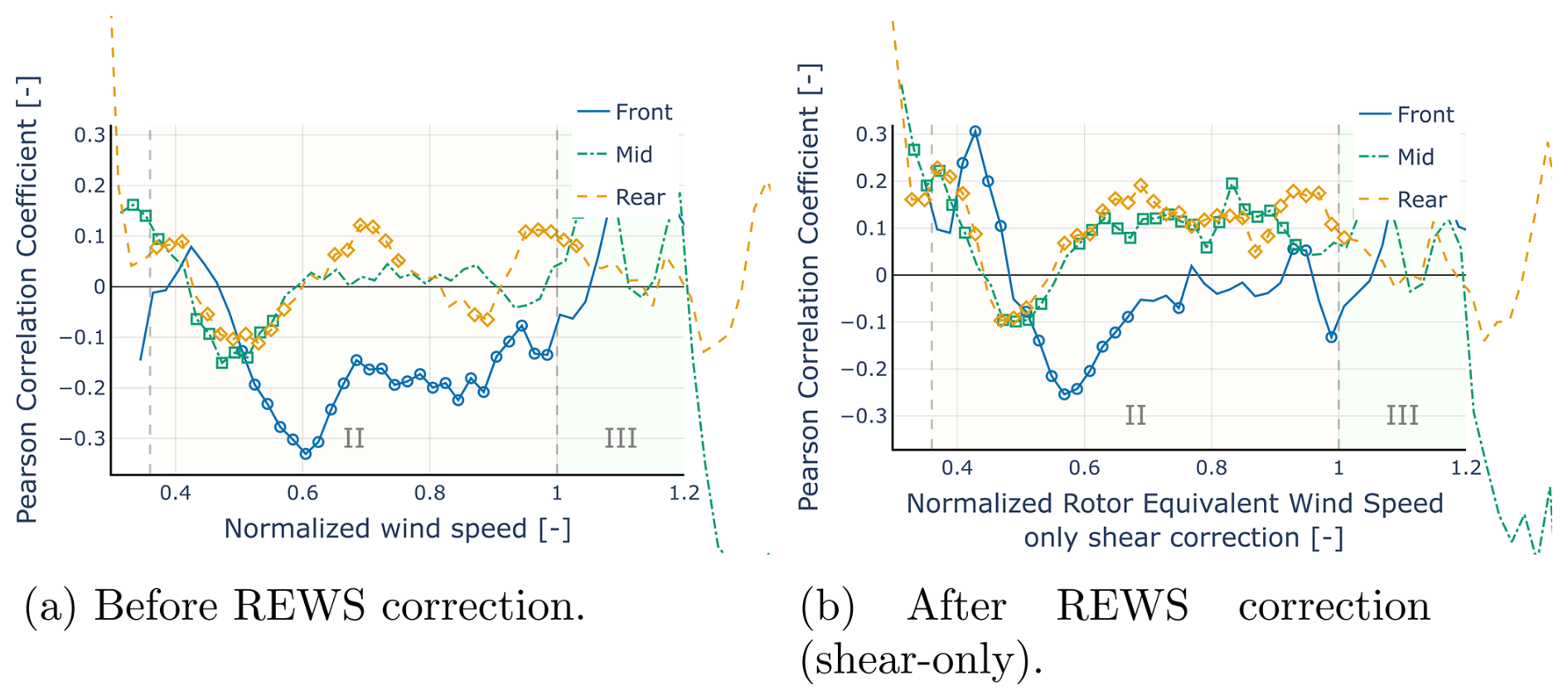
Figure C1 Directional sector robustness check for shear in the central 30° sub-sector. The figure shows the correlation between wind shear α and active power deviation PD for the front, middle, and rear sections as a function of normalized wind speed: (a) before REWS correction and (b) after REWS correction using the shear-only formulation. Markers indicate statistically significant correlations (p<0.05). The section-wise sign patterns and contrasts remain consistent with the wide-sector analysis in Sect. 4, although the curves are noisier because of the reduced sample count in the narrower directional sector.

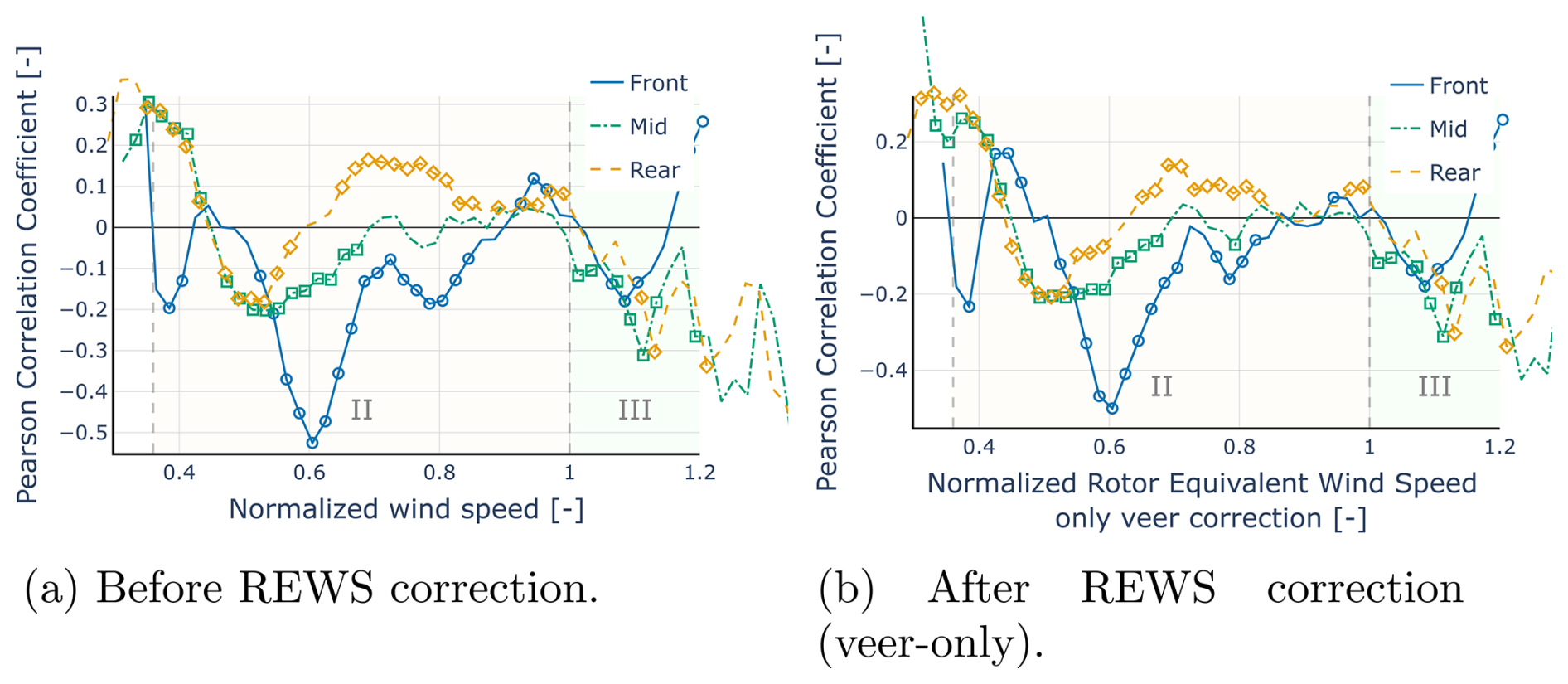
Figure C2 Directional sector robustness check for veer in the central 30° sub-sector. The figure shows the correlation between wind veer β and active power deviation PD for the front, middle, and rear sections as a function of normalized wind speed: (a) before REWS correction and (b) after REWS correction using the veer-only formulation. Markers indicate statistically significant correlations (p<0.05). The section-wise sign patterns and contrasts remain consistent with the wide-sector analysis in Sect. 4.

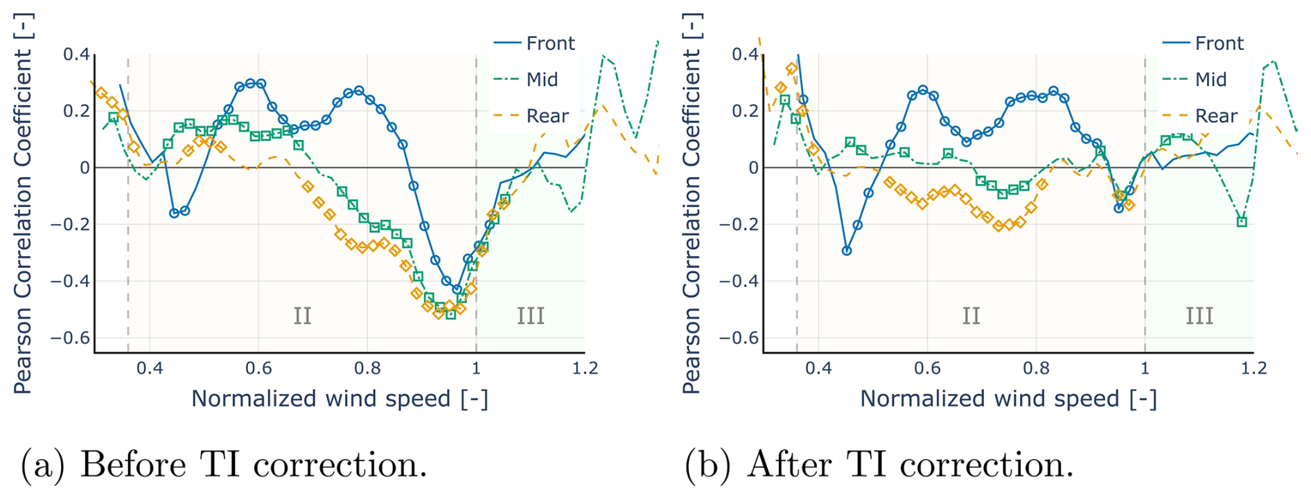
Figure C3 Directional sector robustness check for turbulence intensity (TI) in the central 30° sub-sector. The figure shows the correlation between TI and active power deviation PD for the front, middle, and rear sections as a function of normalized wind speed: (a) before TI correction and (b) after TI correction. Markers indicate statistically significant correlations (p<0.05). The qualitative wind speed dependence and the front–middle–rear contrasts remain consistent with the wide-sector analysis in Sect. 4.