Modelling global offshore turbulence intensity including large-scale turbulence, stability and sea state

This study delivers a method and datasets for a global offshore atlas for turbulence intensity (TI) from 10 to 200 m. The method includes both surface-driven three-dimensional boundary-layer turbulence and large-scale two-dimensional turbulence. This systematically includes the effect of large-scale eddies, particularly at weak wind conditions, and hence significantly improves TI in weak to moderate wind conditions. This method describes water roughness length through a dependence on wave age and wind speed, which is suitable for moderate to strong wind conditions. The method also includes stability dependence through the Obukhov length. Based on theories and measurements in literature, algorithms for TI have been calibrated for heights up to 200 m. We use the ERA5 atmospheric and wave data to demonstrate the use of the method and create a global dataset. The results show satisfactory agreement with measurements and data from the literature.

1 Introduction

Turbulence intensity (TI) is one of the most used parameters in wind energy. For example, it is needed to make decisions about the turbine class for a particular place, as required by the IEC-61400 standard (IEC, 2019). It is required to calculate loads and fatigue. It is also an input parameter for engineering wake modelling.

The most direct way to obtain TI is through wind speed measurements, from which the standard deviation and the mean are calculated during a given period T. For wind speed close to the ground, T is typically 10 min to 1 h. Cup anemometers, and lidar and sonic anemometers are often used to measure TI, with sonic anemometers usually providing the most reliable turbulence data due to their fast response to flow fluctuations, but the associated cost is also the highest.

Measurements are generally expensive to collect, particularly for offshore conditions due to costs related to e.g. operation, maintenance, and data transfer. Traditionally, met-mast or LIDAR are installed to measure the wind conditions for e.g. a year or more before the wind farm is being built. With the rapid and large-scale development of offshore wind energy, there is often limited time to take such measurements, and therefore the information on TI relies heavily on modelling.

When there is a lack of measurements, TI needs to be modelled. The Global Atlas for Siting Parameters (GASP) project (Larsén et al., 2022) provided a near-global modelled dataset of TI at a spatial grid spacing of 275 m from a height of 10 to 150 m. This dataset includes both land and water areas, with water areas reaching 200 km from coastlines, leaving most of open ocean excluded. The calculation of TI over water used the mean wind statistics from Global Wind Atlas data (Davis et al., 2023) data as input to the Kaimal turbulence model (Kaimal et al., 1972), with the surface roughness length z₀ described through the Charnock formulation. The dataset has been applied in the GASP project for defining turbine classes and thus only the moderate to strong wind ranges were used and validated.

This study aims to improve the methodology and datasets for TI for offshore conditions from the GASP project, covering all global offshore areas and addressing also low to moderate winds in addition to moderate to strong wind conditions, as in GASP.

The IEC (2019) standard suggests a simple monotonic decrease of TI with wind speed hub height U:

$$\begin{array}{}\text{(1)}& {\mathrm{TI}}_{\mathrm{IEC}}=I_{\mathrm{ref}}\left(\mathrm{0.75}+{\displaystyle \frac{\mathrm{5.6}}{U}}\right),\end{array}$$

where 5.6 is in m s⁻¹. Equation 1 is obviously only valid over land, because over water it is expected that the surface becomes rougher as the winds increase, contributing to the higher intensity of turbulence in stronger winds, which is supported by measurements (Wang et al., 2014; Christakos et al., 2016; Jeans, 2024).

Wang et al. (2014) developed algorithms from boundary-layer surface scaling laws, where TI is a function of stability and boundary-layer height (z_i), and depends on roughness length z₀, surface momentum and heat fluxes. To take into account the wave effect, they used the Charnock formulation for the roughness length $z_{\mathrm{0}}={\mathit{\alpha }}_{\mathrm{ch}}{u}_{*}^{\mathrm{2}}/g$, where α_ch is the Charnock parameter, for which a typical value of 0.011 is taken. Thus, TI increases with wind speed over the water. The details of the equation for TI from Wang et al. (2014) are included in Appendix A (Eq. A1).

The ISO (2015) standard recommends an increase of TI with wind speed and a decrease with height:

$$\begin{array}{}\text{(2)}& {\mathrm{TI}}_{\mathrm{ISO}}=\mathrm{0.06}\left(\mathrm{1}+\mathrm{0.43}{\displaystyle \frac{U}{\mathrm{10}}}\right){\left({\displaystyle \frac{z}{\mathrm{10}}}\right)}^{-\mathrm{0.22}},\end{array}$$

where U is the wind speed at height z.

Similar relationships between TI and U have been empirically derived through measurements. Before the ISO standard, Andersen and Løvseth (2006) used measurements from the Frøya site and proposed several similar expressions with U scaled with 10 m s⁻¹ and z scaled with 10 m: $(z/\mathrm{10}{)}^{-\mathrm{0.2}}$, primarily for the wind speed range of about 10 to 26 m s⁻¹. The “linear model” from Andersen and Løvseth (2006) reads

$$\begin{array}{}\text{(3)}& {\mathrm{TI}}_{\mathrm{Lin}}=\mathrm{0.087}\left(\mathrm{1}+\mathrm{0.302}\left({\displaystyle \frac{U}{\mathrm{10}}}-\mathrm{1}\right)\right){\left({\displaystyle \frac{z}{\mathrm{10}}}\right)}^{-\mathrm{0.2}}.\end{array}$$

The other two models, the “modified Vickery model” and the “drag coefficient model”, are included in Appendix A (Eqs. A2 and A3).

The expressions from the ISO standard, from Wang et al. (2014) and from Andersen and Løvseth (2006) do not intend to include the decreasing dependence of TI on wind speed under lower wind speed conditions. Wang et al. (2014) added such a dependence at lower wind speed by imposing climatological unstable stratification, which corresponds to stronger vertical mixing and hence larger turbulence intensity.

This decreasing dependence of TI on U at low wind speeds was considered in Christakos et al. (2016) when deriving an empirical relation based on measurements from the FINO masts:

$$\begin{array}{}\text{(4)}& {\mathrm{TI}}_C=c_{\mathrm{1}}U+c_{\mathrm{2}}+{\displaystyle \frac{c_{\mathrm{3}}}{U}}.\end{array}$$

The height dependence of TI is not explicitly included in the expression above but considered through the set of coefficients c₁, c₂ and c₃. For the FINO cases, two sets of coefficients for each site were derived for 30 and 100 m, respectively.

The study of Jeans (2024) could be considered a summary for the above expressions, including the increase of TI with U for moderate to strong winds, a decrease for light winds, and a height dependence of TI similar to the ISO relationship and the Frøya expressions:

$$\begin{array}{}\text{(5)}& {\mathrm{TI}}_{\mathrm{Jeans}}=\left(a_{\mathrm{1}}{\displaystyle \frac{U\left(z\right)}{\mathrm{10}}}+a_{\mathrm{2}}+a_{\mathrm{3}}{\left({\displaystyle \frac{U\left(z\right)}{\mathrm{10}}}\right)}^{-\mathrm{1}}\right){\left({\displaystyle \frac{z}{\mathrm{10}}}\right)}^{-\mathrm{0.22}},\end{array}$$

where a₁=0.035, a₂=0.0089 and a₃=0.0402 are the default values. The coefficients a₁, a₂ and a₃ can be tuned to represent site-specific data, and different values for the three coefficients are also provided for different stability conditions. This expression has been validated in Jeans (2024) with data up to 82 m.

In the above-mentioned TI expressions, only the scaling modelling approach from Wang et al. (2014) is based on physics arguments; the others are empirical, driven by fitting to measurement. This has caused a large variety of sets of coefficients to these expressions, depending on the sites and sometimes measurement heights.

With respect to the application of physics, high-fidelity models are sometimes used to calculate turbulence parameters from which TI can be calculated, such as the large-eddy simulation (LES). Due to its high computational cost, it can only be used for a very limited area, over a short period or in idealised settings. Mesoscale modelling outputs, although by design are not capable of resolving turbulence, are sometimes post-processed to match expected results e.g. in Tai et al. (2023).

In this study, we create a global offshore atlas for TI using a new and cost-effective approach that is based on physical principles. As a first step, we model the turbulence from 1 h to 10 Hz. Usually, the calculation of turbulence and hence TI considers only surface-driven three-dimensional (3D) turbulence. The 3D turbulence is described through spectral models through, for instance, the Kaimal model (Kaimal et al., 1972), the Mann model (Mann, 1994) and the various spectral models reviewed in Veers (1988). The dotted black curves in Fig. 1 show examples of the wind speed power spectra driven by the 3D turbulence at the site Høvsøre at two heights (refer to Sect. 2.1 for details of this figure). The Kaimal model requires input of surface information such as z₀ or u_*, and the Mann model requires turbulence spectra (either from measurements or from other models) as input to further calculate the three-dimensional flow. In most cases, these models are used under the assumption of neutral stability. In common, these models (represented by the black curves in Fig. 1) do not include wind fluctuations from the larger-scales (blue curves for frequency f lower than approximately 10⁻³ Hz). With the current offshore wind energy development and deployment, wind farm clusters can be of the size of several hundreds of square kilometres, and the tallest wind turbine has a hub height of about 185 m, reaching a height of 310 m with rotors (26 MW turbine). At those scales, including the contribution of large-scale turbulence is necessary and is listed as one of the “grand challenges” for the application of wind energy in the latest review article on this subject by Kosović et al. (2026).

The study of the large-scale wind fluctuation dates back to the early 1950s (Panofsky and der Hoven, 1955), followed by several studies throughout the time, including Kraichnan (1967), Charney (1971), Nastrom et al. (1984), Nastrom and Gage (1985), and Lindborg (1999). The idea of the superposition of the large-scale and local turbulence was brought up by Kim and Adrian (1999) and argued in Högström et al. (2002). Larsén et al. (2016) demonstrated the validity of the theory in the spectral gap region through measurements. This strongly suggests that the large-scale and local turbulence are only weakly correlated, if correlated at all in the gap frequency range. A model of superposition of the two components is demonstrated to be able to reproduce the spectral behaviour across the microscale, spectral gap and mesoscale range. There have been several expressions in the literature for the large-scale wind fluctuation e.g. “two-dimensional turbulence” (Kraichnan, 1967; Lindborg, 1999), “geostrophic turbulence” (Charney, 1971), “mesoscale turbulence” (Muñoz-Esparza et al., 2014) or simply “mesoscale fluctuation” (Cheynet et al., 2018). In this study, we follow Kraichnan (1967) and Lindborg (1999), and use the expression “two-dimensional (2D) turbulence”.

Thus, this study will take into account the contribution of the large-scale 2D turbulence, using the full-scale model provided by Larsén et al. (2016). In addition to the 3D and 2D turbulence, our calculation also includes the effect of stability, sea state and height dependence calibrated up to 200 m. The outcome of the method is a look-up table (LUT). We call the method developed here the “LUT” method.

The output is valuable for an initial evaluation of the cost related to the design of the wind turbine and the wind farm, particularly for measurement-sparse regions. The output variables include the mean characteristics of TI, the 90th percentile and the standard deviation of the TI-standard deviation σ_σ of TI.

The method is introduced in Sect. 2. Data used for demonstrate the method for an example global calculation are introduced in Sect. 3.1. Data and analysis from previous studies that are used for validation of the method are presented in Sect. 3.2. Results are shown in Sect. 4, followed by discussions and conclusions in Sects. 5 and 6, respectively.

2 Method for calculation of turbulence intensity

To calculate the turbulence intensity (TI), we start with its definition here by

$$\begin{array}{}\text{(6)}& \mathrm{TI}={\mathit{\sigma }}_U/\stackrel{\mathrm{‾}}{U},\end{array}$$

where $\stackrel{\mathrm{‾}}{U}$ is the mean wind speed and σ_U is the standard deviation of the wind speed. Note that in practice, sometimes it is the standard deviation of the wind components rather than the standard deviation of the wind speed that is used to define the turbulence intensity.

In the absence of measured high-frequency time series of wind speed, we calculate σ_U by integrating the turbulence spectrum model for the wind speed from a lower cutoff frequency f₁ to a higher cutoff frequency f₂, so

$$\begin{array}{}\text{(7)}& {\mathit{\sigma }}_U={\left(\underset{f_{\mathrm{1}}}{\overset{f_{\mathrm{2}}}{\int }}S\left(f\right)\mathrm{d}f\right)}^{\mathrm{1}/\mathrm{2}},\end{array}$$

where S(f) is the turbulence power spectrum for wind speed, the modelling of which is introduced in Sect. 2.1. In boundary-layer turbulence, f₁ is a value in the spectral gap, typically (10 min)⁻¹ or (1 h)⁻¹, while f₂ is a value in the inertial dissipation range e.g. 10 Hz, corresponding to a time series sampled at 20 Hz, which is typical for sonic measurements.

The following subsections explain how both the effects of the typical boundary-layer turbulence (the 3D turbulence) and large-scale variability (the 2D turbulence) are included in the calculation of TI (Sect. 2.1), how the stability effect is included in the algorithms (Sect. 2.2), how the sea state dependence is introduced through parameterisation of z₀ as a function of wave age $c_{\mathrm{p}}/u_{*}$ (Sect. 2.3), how the 90th percentile of TI is calculated (Sect. 2.4) and how the height dependence is added and calibrated (Sect. 2.5).

These algorithms will then be run by using a set of corresponding parameters defined in specific ranges, thus constructing a final LUT with broad ranges of wind, wave and stability conditions combined. The set of parameters and their respective ranges are (1) wind speed at 10 m from 0.1 to 45 m s⁻¹, (2) wave phase velocity at peak frequency c_p from 0.1 to 30 m s⁻¹, (3) stability parameter $z/L$ at 10 m from −3 to 3, (4) 12 wind sectors and (5) height z=10, 50, 100, 150 and 200 m.

For application at a given site, with input of wind speed at a given height (U_z), wave phase velocity (c_p) and stability ($z/L$ at 10 m), we can find the corresponding TI from the LUT.

In this study, we use the fifth generation ECMWF reanalysis data (ERA5) (Hersbach et al., 2020), to demonstrate how these algorithms can be applied globally; the details and preparation of the ERA5 data are provided in Sect. 3.

2.1 Adding large-scale turbulence

As mentioned previously, usually when calculating variance and thereafter standard deviation and turbulence intensity, one integrates Eq. (7) from f₁=  (10 min)⁻¹ or f₁ = (1 h)⁻¹ to f₂=10 Hz.

Figure 1 illustrates the concept of the 3D and the 2D turbulence. The data in Fig. 1 are exported from the study of Larsén et al. (2016) (please refer to that study for the details of the data). The blue curves are the mean spectra from long-term sonic anemometer measured wind speed at 10 m (Fig. 1a) and 100 m (Fig. 1b). The Høvsøre site is located on the west coast of Denmark, where the winds from the west, namely the sea, dominate. The prevailing winds at 100 m represent the sea condition, while 10 m is sometimes affected by the underlying land. Over sea, the spectra will resemble more Fig. 1b, where the 3D turbulence is in general rather weak due to the smooth water surface, and therefore the relative contribution from 2D turbulence is bigger.

The dotted black lines show the typical boundary-layer 3D spectra for wind speed. For f<f_p, with f_p (the peak frequency of the boundary-layer spectrum of wind speed), the Kaimal model shape suggests a saturation of power spectrum at lower frequencies, shown as a 1 : 1 slope in the plot of fS(f) vs f in log-log coordinates:

$$\begin{array}{}\text{(8)}& f{S}_{\mathrm{1},u}\left(f\right)={\displaystyle \frac{\mathit{\alpha }\mathrm{102}{u}_{*}^{\mathrm{2}}fz/U}{(\mathrm{1}+\mathrm{33}fz/U{)}^{\mathrm{5}/\mathrm{3}}}},\end{array}$$

where U is the mean wind speed, z is the height and α=1 by default. S₁ is for the 3D turbulence, and here u is referring to the streamwise wind component, whose spectrum is very similar to that of the wind speed.

The dashed green curves are the spectral model for the large-scale variability of wind speed from Larsén et al. (2013):

$$\begin{array}{}\text{(9)}& f{S}_{\mathrm{2},U}\left(f\right)=a_{\mathrm{1}}{f}^{-\mathrm{2}/\mathrm{3}}+a_{\mathrm{2}}{f}^{-\mathrm{2}},\end{array}$$

where $a_{\mathrm{1}}=\mathrm{3}\times {\mathrm{10}}^{-\mathrm{4}}$ m² s${}^{-\mathrm{8}/\mathrm{3}}$ and $a_{\mathrm{2}}=\mathrm{3}\times {\mathrm{10}}^{-\mathrm{11}}$ m² s⁻⁴ are derived from offshore climatological wind datasets. S₂ is for the 2D turbulence.

The purple curve is a superposition of the Kaimal model and the large-scale variability from Larsén et al. (2016):

$$\begin{array}{}\text{(10)}& f{S}_u\left(f\right)=f\cdot \left(S_{\mathrm{1},u}\left(f\right)+S_{\mathrm{2},U}\left(f\right)\right).\end{array}$$

The good agreement between the purple (model) and blue curves (measurements) suggests the success in bridging the 2D and 3D turbulence calculation using Eq. (10) – the full-spectrum model in the gap region.

The scales of 1 h and 10 min are marked in vertical grey lines in Fig. 1. If the integration of Eq. (7) uses the dotted black curves for the 3D turbulence only, using f₁=  (1 h)⁻¹ gives slightly larger variance and hence slightly larger TI than using f₁=  (10 min)⁻¹. However, the dotted black curves obviously miss out significant amounts of energy for f< (10 min)⁻¹ compared to the blue curves, which are the measurements. Note that the curve from measurements is well described by the model (Eq. 10, the purple curve). In this study, we use the purple curve for the integration of the power spectrum, with f₁=1 h⁻¹ and f₂=10 Hz, thus adding the large-scale turbulence.

Due to the similarity of the spectrum of the wind speed U and the along-wind component u, we refer to the wind speed in this study.

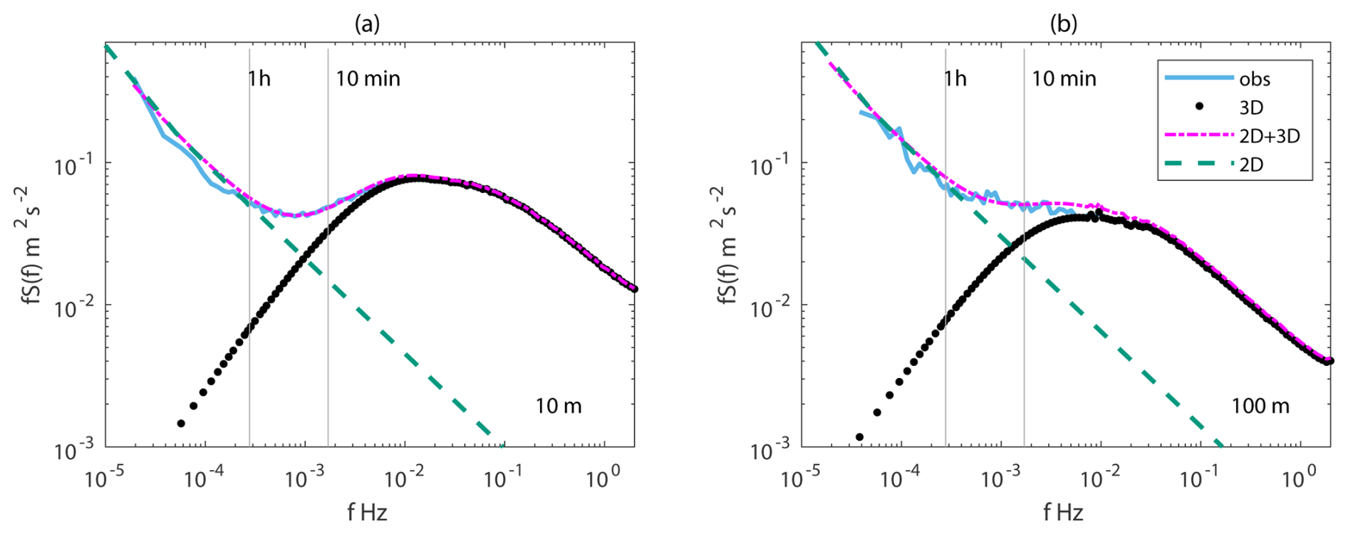
Figure 1 Illustration of the effect of large-scale wind variation on the variance from the gap region using data from Høvsøre (Fig. 8b, d from Larsén et al., 2016, with line colours edited). The power spectra of wind speed is plotted for (a) 10 m and (b) 100 m. The scale of 1 h and 10 min are marked with thin grey lines. The spectra from the measurements are shown in the blue curve, the 3D turbulence for f<f_p is shown as the Kaimal model in black dots (the 3D turbulence for f>f_p is from measurements), the dashed dark-green curve is the mesoscale spectral model from Larsén et al. (2013) (here Eq. 9) and the purple dash-dotted curve is the 2D + 3D turbulence model.

2.2 Adding stability effect

Atmospheric stability is introduced in the calculation through the wind speed profile:

$$\begin{array}{}\text{(11)}& U\left(z\right)={\displaystyle \frac{u_{*}}{\mathit{\kappa }}}\left[\ln \left(z/z_{\mathrm{0}}\right)-{\mathit{\psi }}_m\right],\end{array}$$

where ψ_m is the stability function, dependent on the Obukhov length scale $L=-u_{*}^{\mathrm{2}}\stackrel{\mathrm{‾}}{\mathit{\theta }}/\left(\mathit{\kappa }g{\mathrm{\Theta }}_{*}\right)$, with κ=0.41 (the Von Kármán constant), ${\mathrm{\Theta }}_{*}=\stackrel{\mathrm{‾}}{w^{\prime }{\mathit{\theta }}^{\prime }}/u_{*}$ and $\stackrel{\mathrm{‾}}{\mathit{\theta }}$ the mean surface temperature in K.

For stable conditions $z/L>\mathrm{0}$, we used

$$\begin{array}{}\text{(12)}& {\mathit{\psi }}_m=-\mathrm{5}z/L,\end{array}$$

and for unstable conditions $z/L<\mathrm{0}$, we used

$$\begin{array}{}\text{(13)}& {\mathit{\psi }}_m=\ln \left({\displaystyle \frac{\mathrm{1}}{\mathrm{2}}}(\mathrm{1}+X^{\mathrm{2}})({\displaystyle \frac{\mathrm{1}+X}{\mathrm{2}}}{)}^{\mathrm{2}}\right)-\mathrm{2}\arctan \left(X\right)+{\displaystyle \frac{\mathit{\pi }}{\mathrm{2}}},\end{array}$$

where

$$\begin{array}{}\text{(14)}& X=(\mathrm{1}-\mathrm{15}z/L{)}^{\mathrm{1}/\mathrm{4}}.\end{array}$$

There are many recommendations in the literature on the coefficients that are used together with the stability parameter $z/L$ in Eqs. (12) and (13); see a summary in Högström (1996).

For neutral conditions ψ_m=0 and U=U_N, where

$$\begin{array}{}\text{(15)}& U_{\mathrm{N}}\left(z\right)={\displaystyle \frac{u_{*}}{\mathit{\kappa }}}\ln (z/z_{\mathrm{0}}).\end{array}$$

Thus the relationship between TI and TI_N (turbulence intensity for the neutral condition) can be derived through Eqs. (11) and (15) accordingly:

$$\begin{array}{}\text{(16)}& \mathrm{TI}={\mathrm{TI}}_{\mathrm{N}}\cdot {\displaystyle \frac{\ln (z/z_{\mathrm{0}})}{\ln (z/z_{\mathrm{0}})-{\mathit{\psi }}_m}}.\end{array}$$

2.3 Adding ocean surface wave effect

The wave effect is added through the roughness length z₀, which is used in the wind profile algorithm in Eq. (11). The roughness of the water surface z₀ is related to the sea state, water fetch and water depth.

In this study, we apply the simple sea state dependence, namely the wind sea, and focus on wind-generated waves in open sea conditions. There are many models to describe water roughness z₀ through parameters of the sea state, such as significant wave height, wave length, wave steepness and wave age; see e.g. Larsén et al. (2019) for a summary. Here we build the sea state dependence on the Charnock formulation, with consideration of the smooth water effect for z₀:

$$\begin{array}{}\text{(17)}& z_{\mathrm{0}}=\mathrm{0.11}\mathit{\nu }/u_{*}+{\mathit{\alpha }}_{\mathrm{ch}}{u}_{*}^{\mathrm{2}}/g.\end{array}$$

The first term on the right-hand side is the smooth flow effect due to viscosity, with ν the viscosity coefficient; it introduces a weak decrease of z₀ with increasing wind speed for light wind conditions. The viscosity effect becomes negligible at moderate to strong winds. For the second term in Eq. (17), we use the parameterisation scheme from Fan et al. (2012) through wave age $c_{\mathrm{p}}/u_{*}$ in connection with the Charnock parameter:

$$\begin{array}{}\text{(18)}& {\mathit{\alpha }}_{\mathrm{ch}}=a(c_{\mathrm{p}}/u_{*}{)}^b,\end{array}$$

where $a=\mathrm{0.023}/{\mathrm{1.0568}}^{U_{\mathrm{10}}}$ and b=0.012U₁₀, with U₁₀ the wind speed at 10 m. The reason for choosing the Fan scheme is based on the study of Larsén et al. (2019), in which they compared six parameterisation schemes with measurements at the Horns Rev site in the North Sea where the Fan scheme provides the calculation of z₀ closest to the measurements.

The friction velocity u_* can thus be obtained through iteration by using Eqs. (15), (17) and (18).

The wave phase velocity at the peak frequency c_p is calculated through the wave dispersion relation through the peak wave number k_p, considering the water depth h:

$$\begin{array}{}\text{(19)}& c_{\mathrm{p}}=\sqrt{{\displaystyle \frac{g}{k_{\mathrm{p}}}}\tanh \left(k_{\mathrm{p}}h\right)}.\end{array}$$

2.4 Adding 90th percentile and standard deviation of TI

The 90th percentile of the distribution of σ_u, σ_u,90, at a given wind speed is a concept relevant for turbine design. The standard deviation of σ_u, σ_TI, at a given wind speed corresponds to the approximately 84.1th percentile.

In the IEC standard, ${\mathit{\sigma }}_{u,\mathrm{90},\mathrm{IEC}}=\mathrm{1.84}\cdot I_{\mathrm{ref}}$ is recommended to be the 90th percentile in relation to the mean value. I_ref is the reference TI at a hub height wind speed of 15 m s⁻¹, which is 0.18, 0.16, 0.14 and 0.12 for turbine type A+, A, B and C, respectively.

Wang et al. (2014) proposed the following expression to be the 90th percentile:

$$\begin{array}{}\text{(20)}& {\mathit{\sigma }}_{u,\mathrm{90},W}=\mathrm{0.0123}\cdot U+\mathrm{0.1221},\end{array}$$

which suggests a narrower spread of TI at higher hub height wind speed because of the inverse dependence on U: ${\mathit{\sigma }}_{u,\mathrm{90}}/U=\mathrm{0.0123}+\mathrm{0.1221}/U$.

Wang et al. (2014) also proposed an expression for ${\mathit{\sigma }}_{{\mathit{\sigma }}_u}$:

$$\begin{array}{}\text{(21)}& {\mathit{\sigma }}_{{\mathit{\sigma }}_u,W}=\mathrm{0.0108}\cdot U+\mathrm{0.1189},\end{array}$$

whose magnitude is slightly smaller than σ_u,90.

Based on measurements from the FINO 1, 2 and 3 masts, Christakos et al. (2016) derived the following expression for the standard deviation of TI varying with wind speed:

$$\begin{array}{}\text{(22)}& {\mathit{\sigma }}_{\mathrm{TI},C}=C_{\mathrm{1}}+C_{\mathrm{2}}\cdot e^{-C_{\mathrm{3}}U}.\end{array}$$

They have provided detailed coefficients C₁, C₂ and C₃, depending on the site (FINO 1, 2 or 3) and height. The difference between sites and height is minor, compared to the natural spread of TI from measurements. The estimate of σ_TI from Christakos et al. (2016) is even larger than σ_u,90 from Wang et al. (2014), suggesting the site-dependence characteristics of these empirical expressions.

We found with measurements from FINO1, 2 and 3 that the difference using the above algorithms for σ_u,90 and σ_TI is small compared with the scatter in the measurements. Both Eqs. (20) and (22) are suitable for adding variation to TI at a given wind speed.

2.5 Adding the height dependence of turbulence variance

Several equations mentioned in Sect. 1 implemented the height dependence of TI. Measurements from the tall masts FINO 1, 2 and 3 suggest an average and approximate linear decrease of TI with a height of up to 100 m; see coloured dots and circles in Fig. 2a.

Over water, the height dependence of the power spectrum is rather simple for the 2D turbulence as the coefficients in Eq. (9) are invariant with height at normal measurement heights, following the analysis of the measurements at Horns Rev in Larsén et al. (2016). However, the height dependence of the 3D turbulence could be complicated. The Kaimal model provides a simple dependence of the power spectrum on z; however, its validity still needs to be verified with measurements in different ranges of wind speed and stability, as well as for heights above the surface layer. Thus, using the Kaimal model directly together with the 2D turbulence can sometimes generate a height dependence deviating significantly from the measurements and from theoretical relations that are based on measurements e.g. those in Fig. 2b. To solve this problem, we define a coefficient α in Eq. (10), which is a function of both wind speed and height, for z≥50 m, to multiply Eq. (8), so that our LUT results are consistent with theoretical relations based on measurements at FINO 1. Appendix B provides a list of expressions of α for different wind speed ranges and different heights used for creating the LUT data.

The variances of wind speed and TI at heights 10, 50, 100, 150 and 200 m are obtained using the LUT. To compare with measurements from the three FINO masts, TI from LUT is organised for three wind speed ranges – 1–30, 1–33 and 1–37 m s⁻¹ – which represent wind speed ranges in the three FINO sites. The TI values at z are normalised by those at 30 m (the approximate lowest measurement height at the FINO masts) and are shown in Fig. 2a (black curves). The height dependence from the ISO and its extended form $(z/\mathrm{10}{)}^{-\mathrm{0.22}}$ is also shown in a similar manner in the same figure (blue curve). Due to different measurement periods, data coverage and meteorological conditions at the three sites, there are some differences between the results from the three locations. Nevertheless, the agreement is striking between them, and there is an overall good agreement between the measurements and the LUT data. The ISO and its extended expressions, with $(z/\mathrm{10}{)}^{-\mathrm{0.22}}$, corresponds to a much stronger decrease of TI with height, particularly in the lowest 100 m, when compared with measurements. At higher elevations it is approaching a similar decreasing rate with height to the LUT results.

To verify our calculations for elevations higher than 100 m, data from a remote sensing technique (e.g. sounding or lidar measurements) can be used. Here we use derivations from two classical studies in Stull (1988) and Högström et al. (2002).

Stull (1988) provided the following height dependence of wind variances:

$$\begin{array}{}\text{(23)}& {\displaystyle \frac{{\mathit{\sigma }}_u^{\mathrm{2}}}{u_{*}^{\mathrm{2}}}}=\mathrm{6}(\mathrm{1}-{\displaystyle \frac{z}{z_i}}{)}^{\mathrm{2}}+{\displaystyle \frac{z}{z_i}}{\displaystyle \frac{\stackrel{\mathrm{‾}}{{u^{\prime }}_{\mathrm{top}}^{\mathrm{2}}}}{u_{*}^{\mathrm{2}}}},\end{array}$$

where $\stackrel{\mathrm{‾}}{{u^{\prime }}_{\mathrm{top}}^{\mathrm{2}}}$ is the variance at the top of the boundary layer. Stull (1988) noted: “Although this ratio ($\stackrel{\mathrm{‾}}{{u^{\prime }}_{\mathrm{top}}^{\mathrm{2}}}/u_{*}^{\mathrm{2}}$) is expected to vary from situation to situation, during the KONTUR experiment (Grant, 1986) it was found to equal 2.0 …”. To show Eq. (23) in the figure, we need to specify a number of variables. If we only show normalised variance σ_u(z) by the values at 10 m, then we only need to specify z_i. Assumptions need to be made to estimate z_i, and here we assume a neutral condition and apply the following expression for the atmospheric boundary layer $z_i=\mathrm{0.3}{u}_{*}/f_{\mathrm{c}}$, with f_c the Coriolis parameter. It should be noted that under neutral and stable conditions, the atmospheric boundary-layer height is often denoted by h, whereas z_i commonly refers to the inversion height under convective conditions. Following Arya (2001), z_i is often taken as an approximation of the planetary boundary-layer height h. For consistency with the cited formulations adopted here, we use z_i as a unified notation for boundary-layer height across stability regimes. The coefficient 0.3 was used following Högström et al. (2002), where no theoretical arguments were provided for why this coefficient was used; this expression nevertheless was suitable for interpreting derived measurement behaviours. In Fig. 2b, we plot ${\mathit{\sigma }}_u\left(z\right)/{\mathit{\sigma }}_u\left(\mathrm{10}m\right)$ for both $u_{*}=\mathrm{0.1}$ and 0.2 m s⁻¹, to show the sensitivity. The use of a range of u_* values brings the analysis to a qualitative level, thus also reducing the importance of the absolute value for the coefficient associated with z_i.

Högström et al. (2002) provided the following theoretical expression for the height dependence of variance ${\mathit{\sigma }}_u^{\mathrm{2}}$ for the “very low wavenumbers”, specified as “range (iii)” in their study:

$$\begin{array}{}\text{(24)}& {\displaystyle \frac{{\mathit{\sigma }}_u^{\mathrm{2}}}{u_{*}^{\mathrm{2}}}}=\mathrm{2.5}+\ln \left({\displaystyle \frac{\mathrm{0.46}{u}_{*}A\mathit{\kappa }}{z{f}_{\mathrm{c}}}}\right),\end{array}$$

where A can be determined through $A=f_{\mathrm{c}}\frac{U}{u_{*}}\frac{\mathrm{1}}{n_{\mathrm{l}}}$ and n_l is the lower frequency limit of the surface eddy range in Hz. This “range (iii)” refers to eddies larger than the spectral gap and relevant for the entire boundary layer. With their measurements in the surface layer, Högström et al. (2002) showed the validity of the above expression in the surface layer down to a couple of metres above the ground. The validity of Eq. (24) at higher elevations requires more measurements to confirm. In the absence of information of stability, in Fig. 2b, we plot ${\mathit{\sigma }}_u\left(z\right)/{\mathit{\sigma }}_u\left(\mathrm{10}m\right)$ for both $u_{*}=\mathrm{0.1}$ and 0.2 m s⁻¹, as well as for A=0.5 and 0.3, to show the sensitivity to these parameters.

Results from the four data sources – our LUT calculation, the ISO expression, Stull (1988) and Högström et al. (2002) – are shown in Fig. 2b, where the vertical distribution of the wind speed variance, normalised by the value at 10 m, ${\mathit{\sigma }}_u\left(z\right)/{\mathit{\sigma }}_u\left(\mathrm{10}\mathrm{m}\right)$, is shown. As introduced before, both $u_{*}=\mathrm{0.1}$ and 0.2 m s⁻¹ are used, and for Eq. (24), A=0.3 and 0.5 are used, to show the variation in connection with the use of the two expressions. In general, deeper boundary layer (corresponding to larger u_* and A) results in a slower decrease of wind variance with height. For comparison, to match the general wind conditions from Stull (1988) and Högström et al. (2002), we extracted the variance from the LUT data for wind speed at 10 m not exceeding 18 m s⁻¹. The ISO expression of the height dependence does not distinguish between wind speed ranges; consistent with Fig. 2a, it provides the strongest decrease with height for z<100 m.

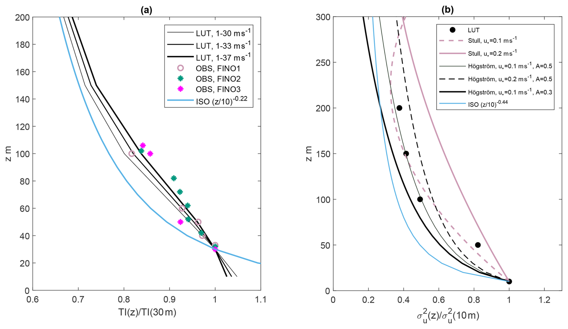
Figure 2 (a) TI normalised with TI at 30 m, with data from measurements at the three FINO sites (see data length from Table 1), ISO expression and LUT method. (b) Comparison of the distribution of wind speed variance with height, normalised with value at 10 m, following the theoretical expressions of Stull (1988) and Högström et al. (2002).

3 Data

In this study, we use ERA5 data (Hersbach et al., 2020) to demonstrate the calculation of global offshore turbulence intensity using the algorithms presented in Sect. 2. Relevant details of the ERA5 data are provided in Sect. 3.1.

At the same time, we use measurements to verify the calculations in the LUT method and use published results on the dependence of TI on U from several studies and sites. The corresponding details are provided in Sect. 3.2.

3.1 The base model data

The ERA5 data are chosen because of the global availability of both atmospheric and wave data. Other atmospheric and wave data can also be used.

In order to match the Global Wind Atlas data layers, including both resource and site parameters (Larsén et al., 2022; Davis et al., 2023), the ERA5 reanalysis from the same period 2008–2017 (both 2008 and 2017 are included) was used here. ERA5 data are available with an hourly time resolution. The meteorological data (wind speed components, 2 m temperature, friction velocity) are available with horizontal spatial grid spacing of 0.25° × 0.25° (about 30 km in the mid-latitude), and the ocean wave data are only available on a 0.5° × 0.5° spatial grid. To avoid unnecessary interpolation of the wave data, our analysis is performed on the wave data grids only.

The following time series from the ERA5 data have been used: meridional and longitudinal wind components at 10 m (U_10 m, V_10 m), wave period at peak frequency (T_p), temperature at 2 m T_2 m, meridional and longitudinal stress components $\stackrel{\mathrm{‾}}{U^{\prime }{w}^{\prime }}$ and $\stackrel{\mathrm{‾}}{V^{\prime }{w}^{\prime }}$, and surface heat flux $\stackrel{\mathrm{‾}}{w^{\prime }{\mathit{\theta }}^{\prime }}$. We also used static bathymetry data.

From the above data, the following variables are derived for 12 directional sectors for all water model grids: (1) mean wind speed at 10 m from the meridional and longitudinal components, (2) frequency of occurrence, (3) mean friction velocity $u_{*}=({\stackrel{\mathrm{‾}}{U^{\prime }{w}^{\prime }}}^{\mathrm{2}}+{\stackrel{\mathrm{‾}}{V^{\prime }{w}^{\prime }}}^{\mathrm{2}}{)}^{\mathrm{1}/\mathrm{4}}$, (4) mean temperature scale ($\stackrel{\mathrm{‾}}{w^{\prime }{\mathit{\theta }}^{\prime }}/u_{*}$) and hence Obukhov length (L), and (5) mean wave phase velocity (c_p) with water depth (h) effect considered through Eq. (19).

3.2 Validation data

In this study, we use 10 min time series of wind speed and standard deviation from FINO 1, 2 and 3 at heights from 30 to about 100 m, to examine the calculation of TI, the 90th percentile and the standard deviation of TI, as well as the dependence of TI on height z. We chose the data periods before the wind farms around them began operations. The periods are specified in Table 1.

Some other measurements are not open source, like the FINO data, so we validate the LUT calculation using the published results on the dependence of the mean TI on the wind speed from Jeans (2024), Peña et al. (2016) and Wang et al. (2014).

Data details of these measurements are provided in Table 1.

Peña et al. (2016)Wang et al. (2014)Jeans (2024)Jeans (2024)Jeans (2024)Jeans (2024)Jeans (2024)Jeans (2024)Jeans (2024)Jeans (2024)Jeans (2024)Jeans (2024)Jeans (2024)

Table 1 Some details of the data from measurements used in the study. “TI–U distribution”: the distribution of mean values of TI in wind speed bins at a certain height, obtained from measurements in the reference studies. Please refer to the references for further details of the data used there. For FINO sites marked with *, we use the results directly from the corresponding reference study.

4 Results

4.1 The look-up table for TI

Using the algorithms presented in Sect. 2, a look-up table (LUT) is generated, where TI is a function of wind speed U, height z, wave phase velocity c_p and stability $z/L$ at 10 m. Figure 3 shows an example of some distributions of TI from the LUT at 10 m. Neutral stability has been applied in Fig. 3a to c, and the stability effect is added in Fig. 3d.

The focus of Fig. 3a is to show the effect of waves on TI. Results from LUT using Eq. (18) in the black dots in Fig. 3a show the variation in TI at a given wind speed, caused by including the wave-age effect through $c_{\mathrm{p}}/u_{*}$. At a given wind speed, for the growing waves, TI increases with $c_{\mathrm{p}}/u_{*}$. The spread in TI is larger at stronger winds. At U₁₀=15 m s⁻¹, the difference caused by $c_{\mathrm{p}}/u_{*}$ in TI is on the order of 0.01. There is a weak decrease of TI with U in light winds due to the smooth flow effect, followed by an increase in TI with U up to approximately 31 m s⁻¹. As can be seen in Fig. 3a, for winds stronger than 31 m s⁻¹, for some groups, TI continues to increase with U but at a lower rate; most often, TI decreases with U again. We still need more measurements at very strong wind conditions to provide a more complete picture of how turbulence behaves there. In the Spectral WAve Nearshore (SWAN) model, the algorithm describing the relation between u_* and U₁₀ adopts the measurements collected in Zijlema et al. (2012): $C_{\mathrm{D}}=u_{*}^{\mathrm{2}}/U_{\mathrm{10}}^{\mathrm{2}}$ is parameterised in terms of U₁₀ following $C_{\mathrm{D}}=(\mathrm{0.55}+\mathrm{2.97}(U_{\mathrm{10}}/\mathrm{31.5}-\mathrm{1.49}(U_{\mathrm{10}}/\mathrm{31.5}{)}^{\mathrm{2}})\times {\mathrm{10}}^{-\mathrm{3}}$. In this expression at high winds U₁₀>31.5 m s⁻¹, C_D saturates, followed by decrease in wind speed, as a simplified effect of the wave breaking process. This results in TI first increasing with U₁₀ and shows similar dependence on the wind speed for U₁₀>31.5 m s⁻¹; see the thick blue curve in Fig. 3a. At the same time, Andreas et al. (2014) recommended the following relationship between u_* and U₁₀: $u_{*}=\mathrm{0.239}+\mathrm{0.0433}\left((U_{\mathrm{10}}-\mathrm{8.271})+\sqrt{\mathrm{0.12}(U_{\mathrm{10}}-\mathrm{8.271}{)}^{\mathrm{2}}+\mathrm{0.181}}\right)$. Their study suggests that the above expression recognises the mechanisms by which heat and moisture cross the air–sea interface through molecular and micro-physical processes at the surface of sea spray droplets, and it has been validated with data for winds up to 25 m s⁻¹ and extrapolated to hurricane wind strength. Compared to the SWAN expression, the Andreas expression suggests a weak increasing dependence of u_* on U₁₀ and, accordingly, when being used together with the Charnock formulation, an increasing dependence of TI with wind speed – shown as the dashed blue curve in Fig. 3a.

Figure 3a shows the calculation using only 3D turbulence (Eq. 8). In Fig. 3b, 2D turbulence is added to the calculation of variance and hence TI. The effect of including the 2D turbulence is shown in Fig. 3b and c in pink dots. In Fig. 3c, the black dots are the same as in Fig. 3a; comparison of the black with the pink dots suggests that the effect of including 2D turbulence is most obvious at light to medium wind speeds, where TI decreases from much higher values with U up to about 7 m s⁻¹. Measurements have consistently shown these high values of TI in low to moderate winds e.g. in Wang et al. (2014), Peña et al. (2016), Christakos et al. (2016) and Jeans (2024).

Based on the values in Fig. 3c, TI is calculated using Eq. (16), with $z/L$ varying from −3 (highest curve) to 3 (lowest curve). Figure 3d shows an example of the impact of stability at a given c_p=10 m s⁻¹.

Corresponding data and LUTs are also made available at 50, 100, 150 and 200 m. Values at heights in between can be interpolated.

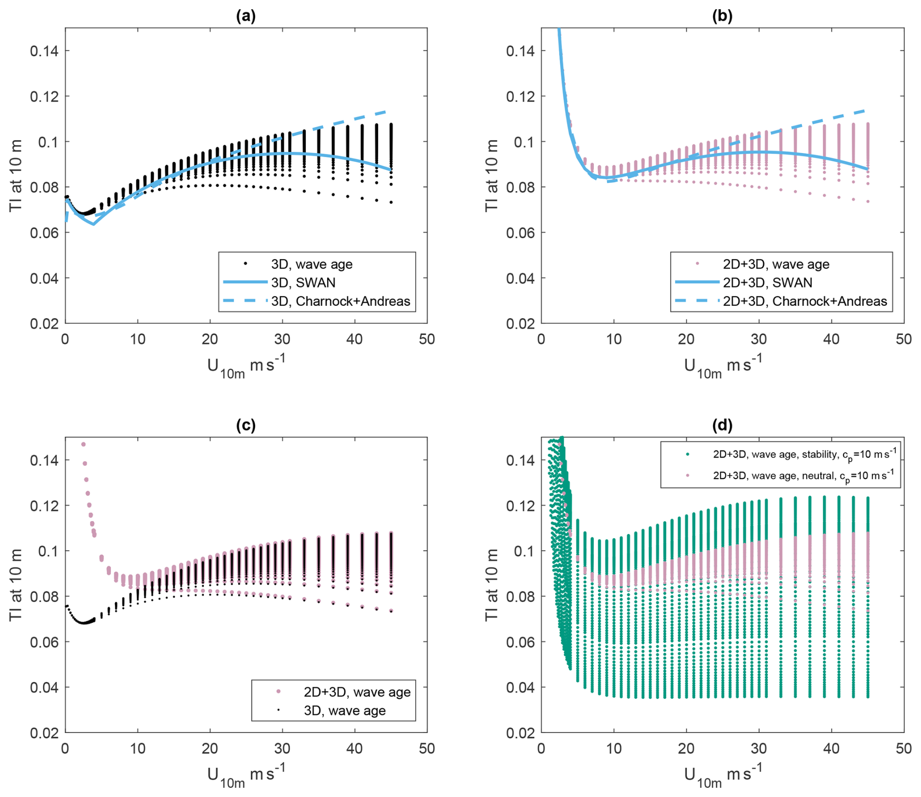
Figure 3 An example of the distribution of the turbulence intensity (TI) with wind speed at 10 m. (a) Includes only micro-scale (3D) turbulence and shows difference of including wave-age dependence, using $z_{\mathrm{0}}=\mathrm{0.011}{u}_{*}^{\mathrm{2}}/g$ together with the Andreas expression (dashed curve), and the SWAN algorithm (solid curve). (b) Similar to (a) but including the large-scale (2D) turbulence. (c) Shows the difference between including and excluding the 2D turbulence in the calculation of TI. (d) The green dots show the effect of stability from $z/L=-\mathrm{3}$ to 3 for the group where c_p=10 m s⁻¹. The pink dots are the same as from (b) and (c), showing the effect of wave age and 2D turbulence but for neutral conditions.

4.2 The global offshore atlas of turbulence intensity

For a given offshore location, if we can get basic information on $z/L$ and c_p, we can use the LUT and identify TI as a function of the wind speed at five heights: z=10, 50, 100, 150 and 200 m. In the absence of certain information, one can always assume neutral stability, skip the wave-age dependence, and use e.g. the SWAN expression or the Andreas expression (e.g. the blue curves in Fig. 3b); the associated uncertainty needs to be assessed, however.

With additional information on the wind speed frequency distribution as a function of each wind condition, we can calculate the corresponding TI distribution at the site. The frequency of occurrence can also be used to weight the calculation in obtaining the mean values of TI.

The information about stability, waves and wind speed distribution can be obtained either from measurements or from modelling. We have prepared global data for these variables based on the ERA5 data. Here we prepared mean values of $z/L$, c_p and wind speed in 12 sectors, along with their occurrence frequencies.

Figure 4a and b show an example of the global distribution of offshore mean values of TI at ERA5 grid points at 10 and 100 m, respectively. To better show the data variability, TI in the range of [0.04, 0.14] is plotted for 10 m (Fig. 4a), and TI in the range of [0.03, 0.1] is plotted for 100 m (Fig. 4b). Here, one can see systematically larger TI at 10 m than at 100 m. Another striking feature is the high TI in the tropical regions; here, based on the ERA5 data, the wind speed is low, and $z/L$ is negative and of large magnitude, suggesting very convective conditions. Thus, these large values of TI are a combination of effect from $z/L$ (see Fig. 3d) and the relatively large 2D turbulence contribution at such low winds (see Fig. 3c). Measurements from this region could be of great value to verify this.

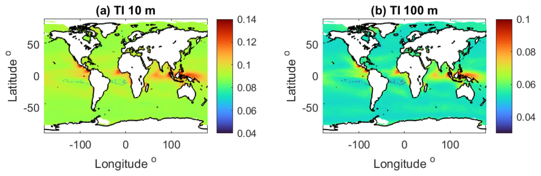
Figure 4 Global atlases of the mean turbulence intensity at (a) 10 m (only values in the range [0.04, 0.14] shown) and (b) 100 m (only values in the range [0.03, 0.1] shown) for offshore grid points, including 2D turbulence, wave age and stability effect. ERA5 data during the period of 2008–2017 are used.

4.3 Validation at sites

4.3.1 TI–U distribution

We compare our calculation with the results from Jeans (2024) at 11 offshore stations, one from Peña et al. (2016) and one from Wang et al. (2014).

First we extracted data from Jeans (2024); their Fig. 5 for the 11 sites and plotted here in Fig. 5a–k, including measurements (red dots) and their calculation using Eq. (5) (dashed blue curves). The mean TI distribution with wind speed based on measurements from Høvsøre (Peña et al., 2016) and from Horns Rev (Wang et al., 2014) are plotted in Fig. 5l and m, respectively. The site names and data heights are shown in the subplots' labels. With the given locations of these sites (Table 1), we extracted the corresponding data from the ERA5-derived atlas as shown in Sect. 4.2, including $z/L$, c_p, wind speed and occurrence frequency in 12 sectors. These data were used to identify the corresponding TI from the LUT. Three of the 11 sites from Jeans (2024) – Frøya Sletringen, Frøya Skipheia and Egmond aan Zee – correspond to ERA5 land grid points as there are small islands nearby. We used the neighbouring water grid point to represent each of the three sites.

The LUT provides data at five heights: 10, 50, 100, 150 and 200 m. To obtain the LUT results at the corresponding heights for the 13 sites, we used the data at two neighbouring heights and applied linear interpolation. The results are shown in solid black curves in Fig. 5.

Our calculation shows overall good agreement with both measurements and Jeans' calculation using Eq. (5) at these sites, and it does not depend on wind speed range. The LUT captures well the variation of TI with U for low to moderate winds, suggesting the success of including the 2D turbulence. On average, the LUT provides an improvement of TI of about 20 % for wind speed greater than 8 m s⁻¹, which is on the order of 0.01, in comparison with Eq. (5), with a larger TI value. In this wind speed range, with the mean TI magnitude less than 0.1, a difference on the order of 0.01 is in general not important, as it does not change the decision of the turbine class. The associated impact on fatigue load is also only a few percentage under normal conditions but could be non-negligible under special conditions such as yaw misalignment. However, such a difference is systematic and should not be ignored.

Among these sites, both the LUT and the Jeans algorithm underestimate TI at Høvsøre. Note that the LUT and the Jeans algorithm assume the site open sea condition. Høvsøre is a coastal site located on land, a few kilometres away from the shoreline. At a height of 100 m, it is assumed that the flow from the ocean represents offshore conditions. The measurement data, shown as red dots in Fig. 5l, were from the water fetch. However, it is not clear if and how much it is affected by the presence of land, which could have contributed to the discrepancies here.

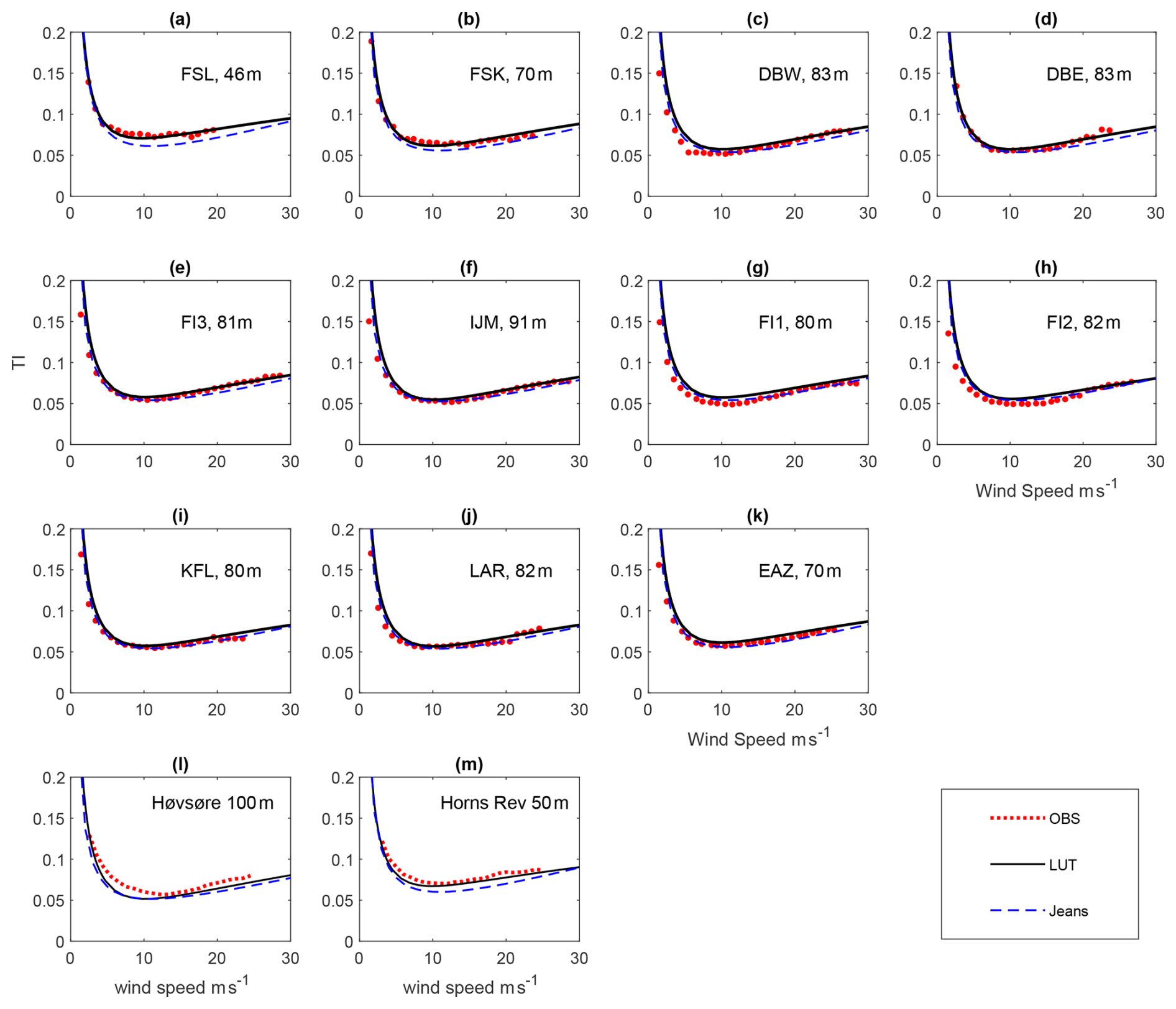
Figure 5 Comparison of TI from the LUT method (black curves), with values from measurements (red dots) and Eq. (5) from Jeans (2024) (dashed blue curves). The measurements are extracted from Jeans (2024) (a–k), from Peña et al. (2016) (l) and from Wang et al. (2014) (m). The names of the sites are (a) Frøya Sletringen, (b) Frøya Skipheia, (c) Dogger Bank West, (d) Dogger Bank East, (e) FINO3, (f) IJmuiden, (g) FINO1, (h) FINO2, (i) Kentish Flats, (j) London Array, (k) Egmond aan Zee, (l) Høvsøre and (m) Horns Rev. The corresponding heights of measurements used in the plot are shown in the subplots.

4.3.2 90th percentile of TI

Using the mean values of wind, wave parameter and stability in 12 sectors derived from ERA5 data as input to the LUT method does not provide a representative scatter of TI. The LUT method here adopts the algorithms from the literature for describing the 90th percentile and the standard deviation of TI. Figure 6 shows an example for the site FINO 1. The mean and 90th percentile of TI at wind speed bins are calculated from measurements, from the IEC standard and from the algorithm provided by Wang et al. (2014). In addition, we also calculated σ_TI at these wind speed bins using the algorithm of Christakos et al. (2016) through measurements from FINO sites. Both the algorithms from Wang et al. (2014) and Christakos et al. (2016) can reasonably well describe the 90th percentile of TI from the measurements here. However, at 30 and 50 m, at wind speeds lower than 10 m, the measurements suggest an even larger variation of TI, which could be partly caused by the fact that we did not take the flow distortion of the tower base into consideration. This effect is clearly not so obvious at 100 m. In Fig. 6a, the mean TI–U curves from the LUT are presented for the FINO 1 site, from 10 to 200 m.

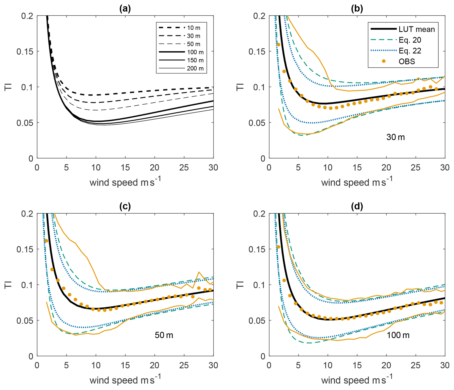
Figure 6 Presentation of TI from the LUT method at FINO 1. (a) Mean values of TI varying with wind speed at six heights from 10 to 200 m. (b) FINO 1 at 30 m, showing mean TI (measurements and LUT), 90th percentile of TI from measurements (orange curve), and derived from Eq. 20 (dashed teal curve) and σ_TI (Eq. 22 (dotted blue curve). (c) FINO 1, similar to (b) but at 50 m. (d) FINO 1, similar to (b) but at 100 m.

5 Discussion

This study provides a method as well as an example database for turbulence intensity for offshore conditions globally, from 10 to 200 m, which are heights relevant for existing turbine types. The data include sector-wise distributions of mean as well as standard deviation of TI as a function of wind speed from calm to gale wind conditions. Note that the current study considers TI in the absence of offshore wind farms. For this reason, direction measurements from the three FINO masts are only used during the period before their surrounding wind farms began operations.

From this method, an LUT is created, where TI can be identified with input of wind speed (U_z), stability ($z/L$ at 10 m), wave phase velocity (c_p) and height (z). The interface for input (U_z, $z/L$, c_p and z) allows the use of data from any source for preparing these variables. It could be from measurements, modelled data or a combination.

Two major contributions from the LUT method are particularly worth highlighting in comparison with previous studies.

The first is the inclusion of the large-scale two-dimensional turbulence, which results in the decreasing dependence of TI with wind speed for lower wind speed ranges. Previously, this part was taken care of by imposing an empirical and artificial dependence e.g. (z^−0.22) or an assumption of climatological unstable conditions at low wind speed (Wang et al., 2014). The large values of TI observed in light winds are often associated with convective conditions. Although we included the stability effect through $\mathit{\psi }(z/L)$ as in Eq. (16), this effect through the sector-wise mean ERA5 values is not obvious. Note that we did not include the stability effect in the derivation using the turbulence spectrum, which is used to calculate σ_U in TI${}_{\mathrm{N}}={\mathit{\sigma }}_U/U_{\mathrm{N}}$. Figure 3c shows that the most significant effect from the 2D turbulence on TI is for small to medium wind speeds. At strong winds, the surface-driven turbulence that is generated using e.g. the Kaimal spectral model under the neutral condition is significant in comparison to the 2D turbulence. At weak winds, the calculated 2D turbulence becomes relatively more important as the Kaimal model generates relatively little turbulence. The inclusion of large-scale wind variability through the 2D turbulence model for weak to medium wind speeds thus compensates for the lack of consideration of stability in the 3D spectrum.

The second is the systematic calibration of height dependence of the calculation of TI up to 200 m with historic-measurements-based studies and measurements from FINO 1. The outcome is satisfactory at the validation sites (Figs. 2a, 5 and 6). The height dependence such as in the ISO standard (z^−0.22) seems to be too strong in the lowest 200 m; see Fig. 2a and b. Note that the validation of TI in (Jeans, 2024) is done mostly at one height.

The LUT method is based on physical principles; it implements algorithms that have been derived from theory and measurements, and validated with measurements. Nevertheless, to carry out the calculation for a global coverage, we used many assumptions and simplified solutions in the chain of algorithms and data. In the following, we discuss the limitations and associated uncertainties in several key assumptions.

First of all, the LUT method includes atmospheric stability effect explicitly through Monin–Obukhov similarity theory (MOST), through Eq. (16). It is known that stability affects the power spectra of wind, and hence the standard deviation of wind speed. The current study did not include any stability effect explicitly in describing the power spectra of wind speed, because it is a very challenging task, particularly for stable conditions. It is relatively easier for unstable conditions due to more organised, larger eddy sizes. Højstrup (1982) suggested an extended spectral model for the unstable condition using a scaling parameter – the boundary-layer height z_i. However, this model has not been tested for scales larger than the gap range. It was shown through a case with the presence of convective open cells in Larsén et al. (2021). The model using z_i is of very limited use in describing the large-scale wind fluctuation, whereas combining 2D and 3D turbulence, in its simple manner, better describes the power spectrum of wind speed for the convective condition. Over water, the stability is less influenced by the diurnal cycles compared to land conditions, except in the coastal zones where land effect is present. Over water, it is mostly influenced by the advection of air masses from another region or from land, associated with weather conditions that likely vary with season. We expect smaller uncertainties associated with stability calculation at strong winds, where it is often close to neutral conditions.

Second, the LUT method uses the Fan scheme (Fan et al., 2012) to include the sea state effect through the roughness length z₀, which is a function of wave age $c_{\mathrm{p}}/u_{*}$ and wind speed. The use of the Fan scheme successfully describes the increasing dependence of TI on wind speed for moderate to strong winds, here validated with measurements up to about 30 m s⁻¹. Note that like most parameterisation schemes for z₀, wave conditions are simplified using the Fan scheme, here Eqs. (17) to (19). For instance, the fetch effect on the wave field is not considered. Only the most dominant wave with a peak frequency is considered when c_p is used. The increasing dependence of z₀ on the wave age is applicable for wind-generated winds while not swell conditions. For a swell-dominated sea state, the waves are detached from the local wind, the wave age $c_{\mathrm{p}}/u_{*}>\mathrm{25}$ or $c_{\mathrm{p}}/U_{\mathrm{10}}>\mathrm{1.2}$, and the corresponding wind speed is often weak. Thus, our neglect of the impact of the swell in our algorithms mainly contributes to the uncertainties in weaker wind conditions. Through the dependence of z₀ (or interchangeably u_* and drag coefficient C_D), our LUT provides the variation of TI with U, including the two schemes: the SWAN and the Andreas schemes. Both schemes are well established, and they use a simple dependence of u_* (or C_D) on U₁₀. Even though the derivation of both addressed possible physics of air–sea interaction, they show contradicting results at the very strong wind conditions (Fig. 3a and b). These reflect the varying challenges in modelling the effect of sea state on atmospheric turbulence in different conditions.

Third, the LUT method calibrates the height dependence of the Kaimal model using measurements from the FINO 1 site and applies it for general use. At the same time, we apply Eq. (15) and MOST to calculate the height dependence of the mean wind speed. This is an oversimplification as Eq. (15) and MOST are expected to be useful in the atmospheric surface layer. Large uncertainty is therefore expected for stable conditions, where the height of the surface layer is very low. Even though the above height dependence descriptions contributed to quite good results at 13 stations (Fig. 5), as well as good agreement with the theoretical expressions from Stull (1988) and Högström et al. (2002), we need more measurements from worldwide locations to provide information for further improvement to reduce uncertainties.

In this study, we used the modelled data for a demonstration of the use of the LUT and hence provided an example of a global dataset. We used the ERA5 data, from which U_z, $z/L$, c_p and z can easily be prepared. One could also use e.g. the New European Wind Atlas (NEWA) data (Dörenkämper et al., 2020) to prepare atmospheric parameters U_z,$z/L$ and z, and use another source for wave parameter c_p. This would of course bring additional uncertainty due to inconsistency in the data sources. Nevertheless, it is worth trying and being validated for individual cases, as a complete set of both atmospheric and wave data is not easy to obtain. If the wave data are absent or proven to be unreliable, one could also neglect the wave-age dependence in the calculation. This corresponds to the solid blue curves in Fig. 3b, instead of the pink dots.

The ERA5 data have a global coverage of both the atmospheric and wave data but are of relatively coarse spatial resolution. This leads to higher uncertainties in coastal zones where the detailed spatial features are not resolved. However, in the LUT method calculations, the ERA5 data can be straightforwardly replaced by other model data with a higher spatial resolution, when possible.

ERA5 surface fluxes are used to calculate the Obukhov length L, which is later used to convert TI from neutral conditions to the corresponding stability conditions. All 13 validation sites are in the North Sea region; the combined data show that there is a dependence of the mean values of $z/L$ on the sectors, with the majority of the data in the range $-\mathrm{0.1}<z/L<\mathrm{0}$ in most sectors and $\mathrm{0}<z/L<\mathrm{0.05}$ in southwest sectors. In general, the averaged stability effect is not significant at the sites shown here, at least from the ERA5 data, but it may be important at other locations.

At the same time, in connection with the use of the global ERA5 wave data, the wave parameters are only available approximately every 50 km for the sites we studied here. This implies that most of the ERA5 data are quite far from the coastlines and are likely more representative for open ocean conditions.

For a global calculation, using a look-up table simplifies the calculation significantly and saves computation. The mean statistics of TI–U relationships and its dependence with height is well captured by the LUT method. To handle the large global ERA5 dataset, only the mean values from 12 directional sectors are stored for wind speed, c_p and L. The spread of TI, associated with wind, stability, wave, fetch and their sector-wise dependence is thus underestimated by using the sector-wise mean values of the ERA5 data. A simple solution is taken here preliminarily through the use of the existing algorithms for describing the standard deviation of TI or the 90th percentile.

In the future, other data with a higher resolution than the ERA5 data can be used to provide the input to apply the LUT method. One could also include more advanced statistics than the sector-wise mean values as input to the LUT method, thus improving the calculation of the spread of TI.

We acknowledge that here the validation of the LUT has only been done to 13 stations in the European seas, which are dominated by similar weather conditions. With the open source codes and data from this study, contributions of data validation from other regions in the world are expected, which will help in identifying issues and finding solutions. For instance, it would be of great interest to see how the LUT performs in areas affected by tropical cyclones, as well as places with special prevalent phenomenon such as water sprouts.

6 Conclusions

This study delivers the look-up table (LUT) method for the turbulence intensity (TI) of offshore conditions. The method describes TI through both the two- and three-dimensional turbulence, making it more suitable for heights above the atmospheric surface layer. At weak wind conditions, this systematically includes the effect of large eddies through the two-dimensional turbulence, which otherwise is neglected in using the three-dimensional turbulence only, under the assumption of neutral stability and weak wind. Accordingly, it captures the decreasing dependence of TI for light to moderate winds. This method describes the roughness length z₀ through dependence on wind speed and wave age, which accurately describes TI for moderate to strong winds, including wave breaking effect. Stability effect is also included. The method for TI can be applied globally and was calibrated to a height of 200 m.

The global data prepared using this method together with the global ERA5 wind and wave data were shown to perform reasonably well with validations from 13 offshore sites and comparison with earlier studies. With a given location, we can find the corresponding ERA5 coordinates and extract the corresponding data. The LUT will then provide TI according to this information at the above-mentioned five heights. If the height of interest is in between those five heights, one can interpolate between neighbouring heights.

This method is flexible to use if one has special data as input. In the absence of other data sources, one can use the global ERA5 data prepared here by providing the coordinate for the site of interest.

Appendix A: Collection of expressions of TI

The detailed expressions for TI from Wang et al. (2014) and Andersen and Løvseth (2006) are provided here. Specifically, the equation of TI from Wang et al. (2014) reads

$$\begin{array}{}\text{(A1)}& {\mathrm{TI}}_{\mathrm{Wang}}={\displaystyle \frac{\mathit{\kappa }{\left[C_{\mathrm{NT}}^{\mathrm{2}}+C_{\mathrm{MX}}^{\mathrm{2}}(-z_i/L{)}^{\mathrm{2}/\mathrm{3}}\right]}^{\mathrm{1}/\mathrm{2}}}{\ln (z/z_{\mathrm{0}})-{\mathit{\psi }}_m(z/L)}},\end{array}$$

where C_NT and C_MX are two constants as approximates for $\mathit{\sigma }/u_{*}$ and $\mathit{\sigma }/w_{*}$, respectively. For neutral and mixed-layer conditions, u_* is the friction velocity and w_* is the convective velocity scale, and it is a function of temperature, surface heat flux and height of the boundary layer z_i, with L as the Obukhov length.

There are several similar expressions in Andersen and Løvseth (2006), primarily for the wind speed range from 10 to 26 m s⁻¹. This includes the “modified Vickery model”

$$\begin{array}{}\text{(A2)}& {\mathrm{TI}}_{\mathrm{Vic}}=\mathrm{0.085}{\left({\displaystyle \frac{U}{\mathrm{10}}}\right)}^{\mathrm{0.421}}{\left({\displaystyle \frac{z}{\mathrm{10}}}\right)}^{-\mathrm{0.2}},\end{array}$$

the “drag coefficient model”

$$\begin{array}{}\text{(A3)}& {\mathrm{TI}}_{\mathrm{Dra}}=\mathrm{0.0857}{\left(\mathrm{1}+\mathrm{0.758}\left({\displaystyle \frac{U}{\mathrm{10}}}-\mathrm{1}\right)\right)}^{\mathrm{0.5}}{\left({\displaystyle \frac{z}{\mathrm{10}}}\right)}^{-\mathrm{0.2}}\end{array}$$

and the “linear model”, which has already been introduced as Eq. (3) in Sect. 1.

The three expressions (Eqs. A2, A3 and 3) provide similar estimates up to a wind speed of 26 m s⁻¹, which describe well the measurements at the Frøya site from about 10 to 46 m. Cheynet et al. (2024) showed the validity of Eq. (3) from 8 m s⁻¹. Above 26 m s⁻¹, there are no measurements, and the linear model gives considerably larger values, which was recommended by the authors for a slightly conservative design approach.

Appendix B: Calculating the height dependence of variance

In the process of calibration using measurements from FINO 1, we added a coefficient α to the Kaimal model expression for u for different z, starting from 50 m and above. The coefficient α is a function of wind speed at each height.

$$\begin{array}{}\text{(B1)}& {\displaystyle }{\mathit{\alpha }}_{\mathrm{50}m}& {\displaystyle }=\mathrm{0.018}U+\mathrm{0.54},U\le \mathrm{10}\mathrm{m}{\mathrm{s}}^{-\mathrm{1}}\text{(B2)}& {\displaystyle }& {\displaystyle }=\mathrm{0.024}U+\mathrm{0.48},\mathrm{10}\mathrm{m}{\mathrm{s}}^{-\mathrm{1}}<U\le \mathrm{32}\mathrm{m}{\mathrm{s}}^{-\mathrm{1}}\text{(B3)}& {\displaystyle }& {\displaystyle }=\mathrm{1.29},U>\mathrm{32}\mathrm{m}{\mathrm{s}}^{-\mathrm{1}}\text{(B4)}& {\displaystyle }{\mathit{\alpha }}_{\mathrm{100}\mathrm{m}}& {\displaystyle }=\mathrm{0.035}U+\mathrm{0.037},U\le \mathrm{35}\mathrm{m}{\mathrm{s}}^{-\mathrm{1}}\text{(B5)}& {\displaystyle }& {\displaystyle }=\mathrm{1.26},U>\mathrm{35}\mathrm{m}{\mathrm{s}}^{-\mathrm{1}}\text{(B6)}& {\displaystyle }{\mathit{\alpha }}_{\mathrm{150}\mathrm{m}}& {\displaystyle }=\mathrm{0.031}U+\mathrm{0.033},U\le \mathrm{35}\mathrm{m}{\mathrm{s}}^{-\mathrm{1}}\text{(B7)}& {\displaystyle }& {\displaystyle }=\mathrm{1.12},U>\mathrm{35}\mathrm{m}{\mathrm{s}}^{-\mathrm{1}}\text{(B8)}& {\displaystyle }{\mathit{\alpha }}_{\mathrm{200}\mathrm{m}}& {\displaystyle }=\mathrm{0.029}U+\mathrm{0.031},U\le \mathrm{35}\mathrm{m}{\mathrm{s}}^{-\mathrm{1}}\text{(B9)}& {\displaystyle }& {\displaystyle }=\mathrm{1.05},U>\mathrm{35}\mathrm{m}{\mathrm{s}}^{-\mathrm{1}}\end{array}$$