50-year wind speed maps for tropical-cyclone-affected regions using best track data

Accurate estimation of extreme wind speeds from tropical cyclones is a significant challenge in regions prone to tropical cyclones. This study presents a method to estimate the 50-year return wind speed at heights relevant to wind turbines. The International Best Track Archive for Climate Stewardship data are combined with the Holland parametric model and the Gumbel distribution to assess extreme winds in three tropical-cyclone-affected regions in the Northern Hemisphere. These regions are Taiwan, Japan, and the east coast of the US. To assess the uncertainty in the results from differing input parameters, Monte Carlo simulations are used. The method aligns with previous studies through the spatial representation of wind speeds and maximum 50-year return wind speeds in Taiwan and Japan that can be attributed to the large sample size of data points located in a limited spatial area. The east coast of the US exhibits spatial fragmentation and only partially aligns to the spatial representation of 50-year return wind speeds from previous studies, which, conversely, is due to the smaller sample size and wider spatial region of which they cover. This study shows that combining International Best Track Archive for Climate Stewardship data with parametric and statistical models provides a practical approach to estimate extreme wind speeds while highlighting the need for an understanding of regional characteristics to ensure reliability of the results.

1 Introduction

Tropical cyclones (TCs) can be a devastating weather event, especially in coastal and offshore regions (Mortlock et al., 2018). Therefore, an assessment of extreme winds is increasingly important due to the current global expansion of offshore infrastructure, including offshore wind farms (Chen and Su, 2022).

The International Electrotechnical Commission (IEC), in standard 61400-1, provides a reference wind speed class specifically for wind turbines in TC-prone regions, known as Class T (International Electrotechnical Commission, 2019). However, it also expresses the fact that the reference wind speed may not cover all regions prone to TCs.

There are a range of methods that have been used in previous studies to assess extreme wind speeds from TCs. For example, many have taken advantage of the International Best Track Archive for Climate Stewardship (IBTrACS) (Knapp et al., 2010; Gahtan et al., 2024). IBTrACS is a state-of-the-art dataset containing information on TC parameters, such as the maximum wind speed, minimum sea level pressure, centre position, and radius of maximum winds (RMW). IBTrACS is widely known and used. Of those using the IBTrACS dataset, select studies such as Ott (2006), Schreck et al. (2014), and Kossin (2018) focus on general TC analysis, whereas others such as Bloemendaal et al. (2020b), Morin et al. (2024), and Xu et al. (2024) focus on the combination of IBTrACS with other datasets to develop new synthetic datasets.

The IBTrACS dataset, however, is not without its limitations. IBTrACS does not provide the entire wind wield but rather a singular value for the maximum wind speed at each given time step. To obtain the entire wind field, parametric models such as the Holland model (Holland, 1980) can be implemented to extrapolate a singular point into a wind field in a computationally efficient way. Parametric models are used across academic and industrial fields to investigate TCs (Arthur, 2021), and the combination of IBTrACS data with parametric models is a well-used method (Ott, 2006; Fang et al., 2020; Wei et al., 2023).

In an attempt to mitigate the damage caused by extreme winds, the IEC standard defines a reference speed for each class of wind turbine. The reference speed is defined as the 10 min wind speed average for a return period of 50 years (U₅₀) at turbine hub height. To align with the IEC standard, this paper focuses on these exact requirements. To calculate U₅₀, generalised extreme value (GEV) is implemented, as previously used by Abild (1994) and Larsén et al. (2015).

The U₅₀ of TCs has previously been studied, but researchers have rather focussed on using reanalysis data, combining IBTrACS reanalysis data with IBTrACS (Anastasiades and McSharry, 2014), combining IBTrACS with more complex models to generate a synthetic dataset (Vickery et al., 2009; Bloemendaal et al., 2020a), or comparing extreme value analysis methods for TCs (Ott, 2006; Kong et al., 2024). Reanalysis datasets can provide useful information on TCs (Kossin, 2015) and other weather phenomena (Mavromatis, 2022; Wang et al., 2023), but they often underestimate the maximum wind speeds of TCs (Li et al., 2024), making it difficult to estimate the potential impact of TCs on offshore infrastructure (Gandoin and Garza, 2024; Liu et al., 2025). Another commonality between previous studies is the primary focus on either a single basin for winds at 10 m (Ott, 2006; Kong et al., 2024) or a limited number of specific latitude–longitude coordinates (Vickery et al., 2009; Bloemendaal et al., 2020a).

One particular study, Larsén and Ott (2022), focussed on overcoming the systematic underestimation of extreme TC wind speed in reanalysis data. The missing wind variability was filled in according to the Climate Forecast System Reanalysis (CFSR) reanalysis data using a spectral correction method. The application of the spectral correction uses the U₅₀ estimation from Ott (2006), which in turn is based upon using the Japanese Meteorological Agency (JMA) track data (a subset of the IBTrACS dataset). This method was applied to two regions: the southwest of the northern Pacific Ocean and the western Atlantic Ocean. This was later adjusted in Imberger et al. (2024) to include two more reanalysis datasets: ERA5 (European Centre for Medium-Range Weather Forecast Reanalysis v5) and MERRA 2 (Modern-Era Retrospective analysis for Research and Applications) for which IBTrACS data are available. However, this study presents no validation through measurements.

This paper focuses on the use of the state-of-the-art IBTrACS data, updates the study of Ott (2006) which was only over the typhoon-affected southwest of the northern Pacific ocean. The regions extended to include the ocean around Taiwan located in the western Pacific Ocean, the ocean around Japan (also located in the western Pacific) and the east coast of the US (ECUS) located in the northern Atlantic. These have been chosen as they encompass most of the regions affected by TCs in the Northern Hemisphere and areas that contain offshore wind development.

The aim of this study is, first of all, to develop a computationally efficient method to derive U₅₀ that can be applied across many different regions, taking advantage of the IBTrACS data. Second, this study investigates the applicability of the IBTrACS data in different regions for the calculation of U₅₀ by recognising regional TC characteristics. Third, this study explicitly accounts for how uncertainties in IBTrACS propagate through to the final U₅₀ results. This paper is a necessary complement to Ott (2006) with its more complete use of IBTrACS data, and to Larsén and Ott (2022) and Imberger et al. (2024) due to the use of IBTrACS data.

Section 2 introduces the method developed to estimate U₅₀ and the accompanying uncertainty analysis using Monte Carlo simulations. Results are presented in Sect. 3, the uncertainty analysis is detailed in Sect. 4, followed by Discussions and Conclusions in Sects. 5 and 6, respectively. A list for abbreviation is provided in the Appendix for readability.

2 Method

This section introduces and discusses the data used in the analysis and the method by which the data have been processed to obtain U₅₀ in three regions.

Below is a brief overview of the steps taken to calculate U₅₀. Each step is explained in more detail in the corresponding sections throughout the paper. Figure 1 shows the workflow of the method.

1. Define the regions of interest. The three regions of focus are Taiwan, Japan, and ECUS. The exact coordinates used to define these regions are described in Sect. 2.2.

2. Select relevant data. A set of data restrictions is applied to the IBTrACS data. These restrictions are that (1) the data point must fall within the region of interest; (2) the data point should contain either the radius of maximum wind (RMW) or the 50 kt radius, the minimum sea level pressure, and the maximum wind speed; and (3) the data point should be over ocean. (2) is required as these are the necessary parameter inputs to the parametric model, and (3) is required as the parametric model used to extrapolate a single data point to a wind field is only valid over the ocean. The parametric model is discussed in point 4.

3. Convert wind speeds to common averaging period. The IBTrACS dataset is a compilation of data from agencies across the globe. Hence, the maximum wind speed is given at different averaging periods. All wind speeds are converted to a 10 min averaging period using the method described in Harper et al. (2010). The 10 min average was chosen as it is used as the reference speed at hub height in the IEC standard 61400-1 (International Electrotechnical Commission, 2019). Details of this conversion process are provided in Sect. 2.3.

4. The Holland model. A 0.25°×0.25° latitude–longitude grid is defined. The grid was defined to be this resolution, as a higher resolution grid requires larger computational resources, and a lower resolution could dilute key features of U₅₀. Once the grid is defined, the Holland model can be used. Using input parameters such as wind speed and RMW, the Holland model can extrapolate a single data point into a wind field. Following this, at each defined grid point, a corresponding wind speed value is assigned. The Holland model wind field is computed for each data point available from IBTrACS, given the data constraints. More information on the Holland model is provided in Sect. 2.4.

5. Scale wind speeds to 100 m height. The Holland model returns wind speeds at gradient height – the height at wind surface friction no longer significantly affects the wind flow. These winds are scaled down to 100 m. Any newly created data points from using the Holland model that now fall over land are removed. This is discussed in Sect. 2.5.

6. Calculate the annual maxima. The scaled wind fields are separated into yearly groups, and the annual maxima are calculated for each grid point. The annual maxima calculation is described in Sect. 2.6.

7. Fit the Gumbel distribution. From the annual maxima, the Gumbel distribution is fitted to estimate U₅₀ at each grid point. This is the final step in this method, which provides a map of U₅₀ for each region. The process is also described in Sect. 2.6.

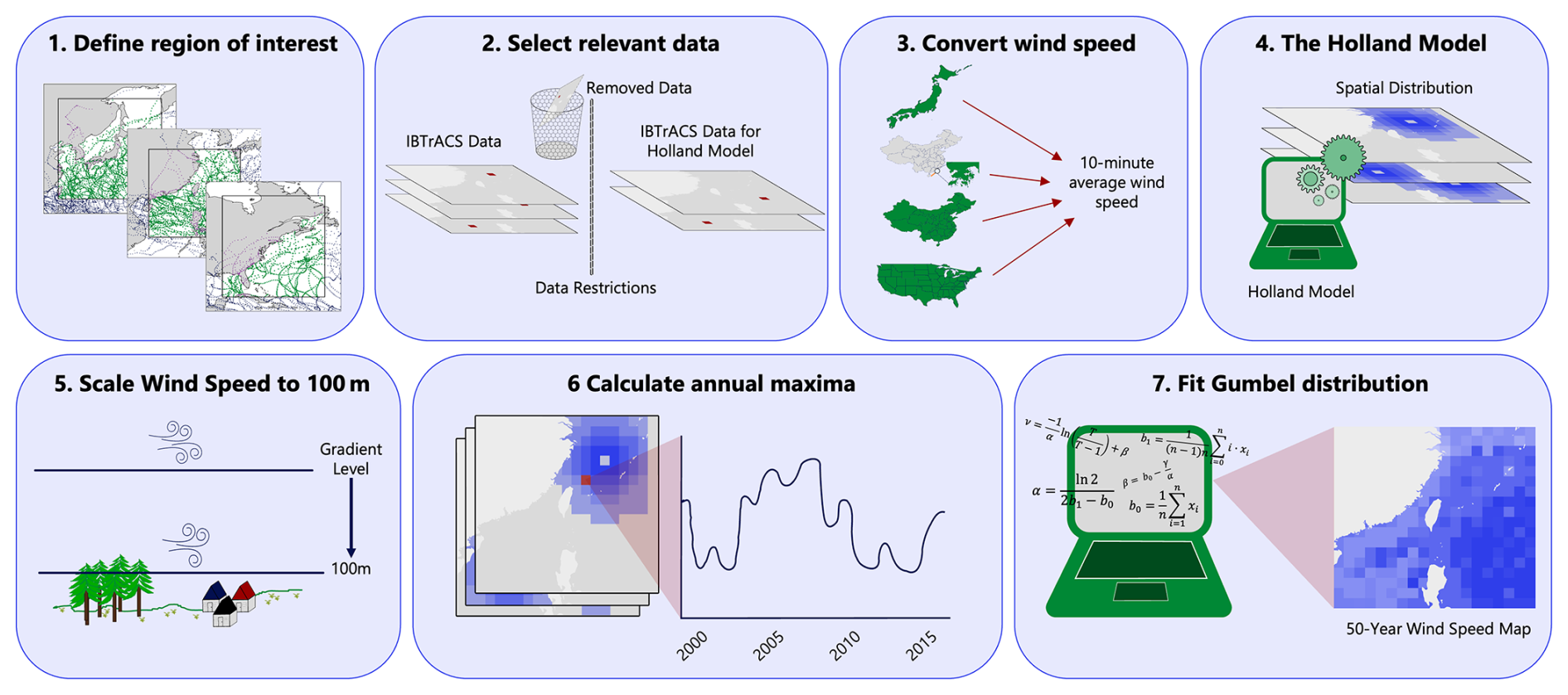
Figure 1 Illustration of seven-step workflow depicting the method used to calculate U₅₀ at 100 m using IBTrACS.

2.1 Data

IBTrACS is a global tropical cyclone dataset maintained by the National Oceanic and Atmospheric Administration (NOAA). NOAA compiles post-storm records of best-estimate TC parameters from multiple regional meteorological agencies, providing information such as storm position, central pressure, and maximum sustained wind speed at regular time intervals (typically every 3 h). At every 3 h time step, new values are provided where possible; however, a spatial realisation of the wind field (or other parameters) is not available. IBTrACS serves as a consolidated and quality-controlled reference for historical TC activity. Table 1 shows which agencies' data are available in IBTrACS, in categories of data temporal resolution; those in bold are used in the following methods in this study. The differences between agencies pose different challenges throughout the analysis and will be detailed throughout.

Table 1 Wind averaging period by agency. Bold entries indicate agencies from which data were used in this study.

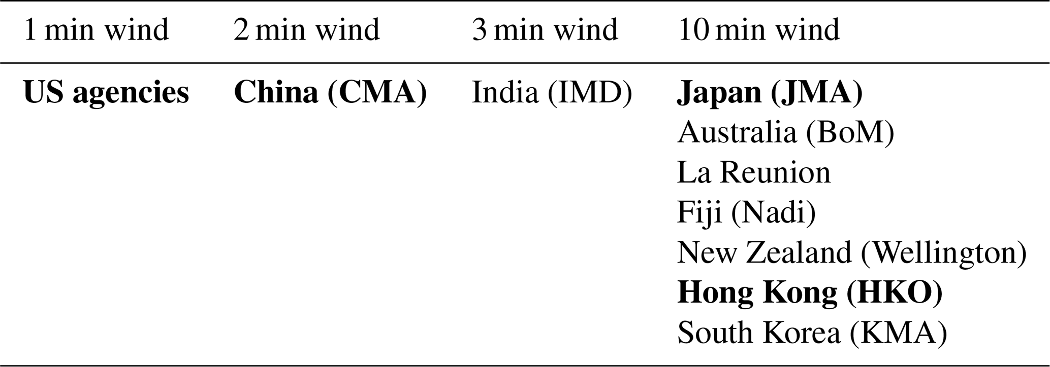
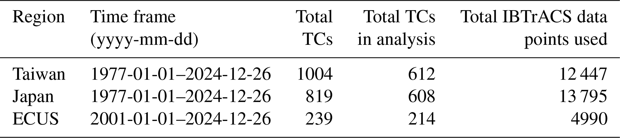
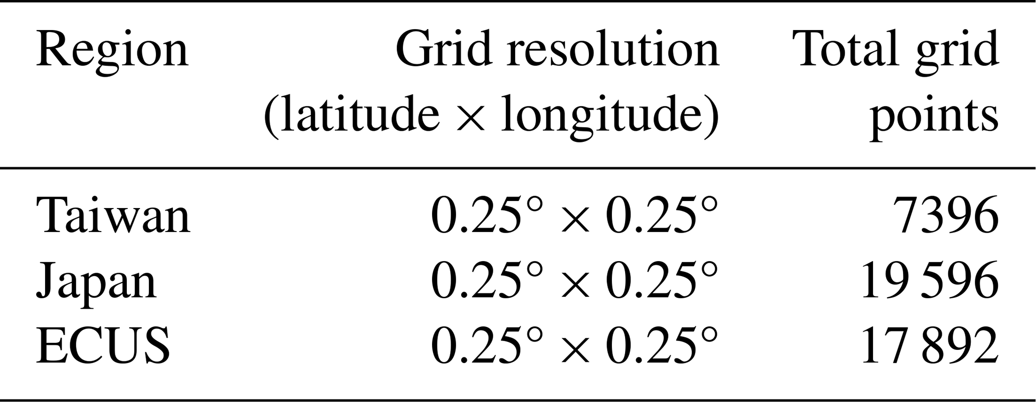
Table 2 shows a comparison between the three regions: the time frame of TCs captured for this analysis, the total TCs in each region for the given time frame, the total TCs that have at least one data point with the needed parameters (maximum wind speed, RMW, minimum sea level pressure), and the number of IBTrACS data points used. The time frame of ECUS is limited by the availability of the RMW parameter and is further explained in Sect. 2.4. Table 3 shows a regional comparison of the grid resolution and the total number of grid points.

Table 2 Regional data comparison.

Table 3 Regional grid comparison.

2.2 Defining the “regions”

While three regions are being evaluated in this study – Taiwan, Japan, and ECUS – the primary focus is the coastal areas, as this is where most offshore structures are located (e.g. Díaz and Guedes Soares, 2020). Given that TCs can be very intense systems, the TC extreme winds can still have a significant impact on areas hundreds of kilometres away from the eye, and therefore there needs to be consideration of the region chosen. The exact extent of how far damaging winds can reach is a complex subject (Weatherford and Gray, 1988; Powell and Reinhold, 2007; Chan and Chan, 2012; Knaff et al., 2021). To ensure all potential TC effects are captured, a wide area has been chosen to evaluate, as shown by Fig. 2a, b, and c. In these figures, a subset of IBTrACS data is shown to illustrate which IBTrACS data points are included in our calculation. A region of approximately 500 km from the most northern, eastern, western, and southern points are included in the map, as shown by the black square. Any data points outside of the black box have been excluded, represented as dark-blue dots in the figure. The purple dots over land are also excluded from this study. The green dots represent included data points.

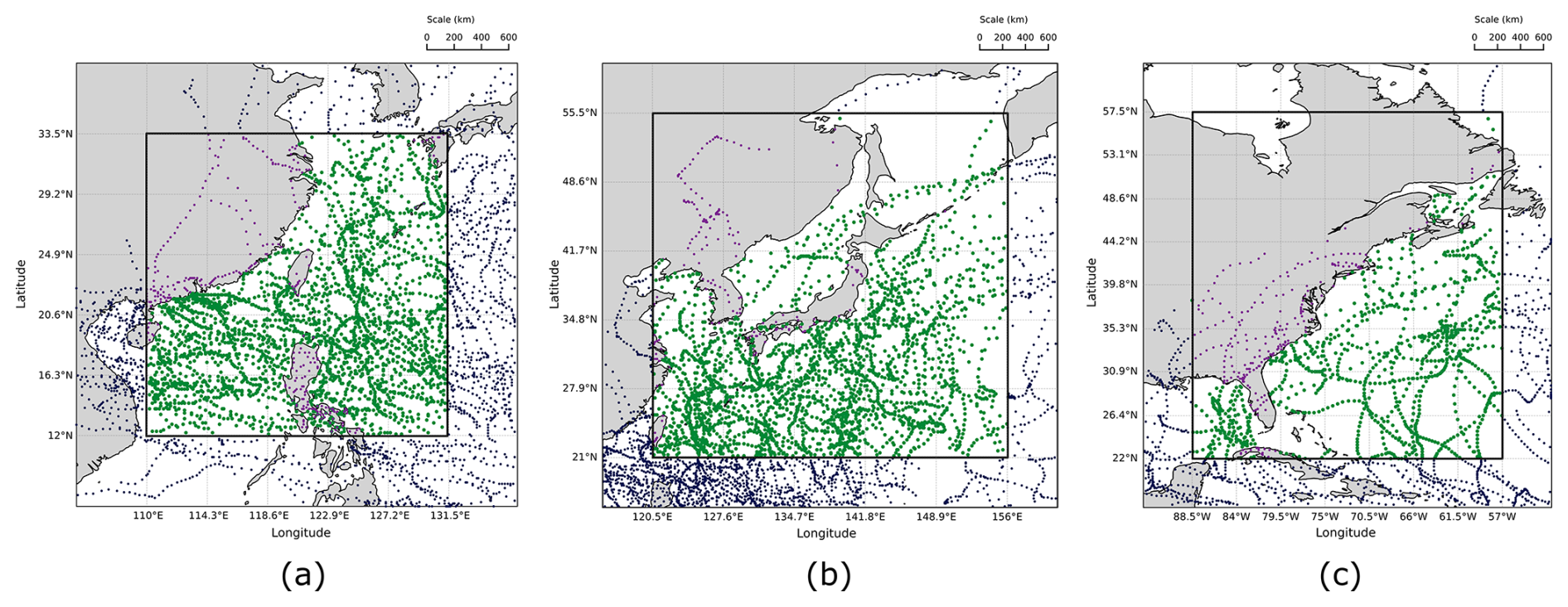
Figure 2 (a) Taiwan region. Subset: TCs in the western Pacific, 1 January 2020 to 1 January 2025. (b) Japan region. Subset: TCs in the western Pacific, 2020–2025. (c) ECUS region. Subset: TCs in the North Atlantic, 2021–2024. Coordinate restrictions and removed data points for each region. The inner black box represents the coordinate restrictions placed on the IBTrACS data. The dark-blue dots represent excluded data points due to being outside the coordinate. The purple dots represent excluded data points due to being over land. The green dots represent data points included in the analysis. Only a subset of IBTrACS data is shown to illustrate which data are excluded.

For the ECUS region, data have been used from the pre-compiled US agencies' variables within IBTrACS. All data for the Taiwan region come from the World Meteorological Organisation Regional Specialised Meteorological Centre in Tokyo. It is operated by the Japanese Meteorological Agency (JMA), responsible for official typhoon forecasts in the western North Pacific. The JMA dataset spans from 1951 to the present. For the Japan region, data from four agencies were combined to maximise the data availability. As previously mentioned, certain parameters are needed, and therefore merging data from different agencies can help to fill data gaps. A hierarchy of preference was established: JMA, HKO, CMA, US. This order of preference is based on the number of available data points for the Japan region, with JMA offering the highest count of data points and the US agencies the least.

2.3 Wind speed conversion

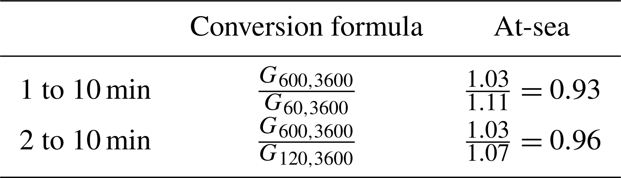
Different agencies report the maximum wind speed of TCs using different averaging periods. To ensure consistency across datasets, all wind speeds have been standardised to a 10 min average to align with IEC standard 61400-1. Shorter averaging periods tend to return higher wind speeds, whereas a longer averaging period results in lower wind speeds as fluctuations of turbulence are smoothed over time. Harper et al. (2010) derived algorithms to convert wind speeds measured at 10 m between different averaging periods. The conversion factors used here are provided in Table 4. The recommended procedure to convert a shorter averaging period to a lower averaging period is as follows:

The wind speed conversion factor (CF) for converting x minute wind speed to y minute wind speed, where x<y, is given by

$$\mathrm{CF}={\displaystyle \frac{G_{y,\mathrm{3600}}}{G_{x,\mathrm{3600}}}},$$

where G_x,3600 is a conversion value that gives the highest x second mean (gust) wind speed (for example, 600 s–10 min) within 3600 s.

Table 4 Wind speed conversion between temporal resolutions of 1 to 10 min, and 2 to 10 min.

2.4 Holland model

The Holland model, developed by Holland (1980), is a conceptual, empirical model to extrapolate one point of data into a wind field. Figure 3 illustrates a singular data point being extrapolated to an entire wind field. The following use of the Holland model follows the method in Ott (2006). First, the B parameter is calculated:

$$\begin{array}{}\text{(1)}& B={\left({\displaystyle \frac{V_{\text{max}}}{K_{\mathrm{M}}}}\right)}^{\mathrm{2}}\cdot \mathit{\rho }\cdot e\cdot {\displaystyle \frac{\mathrm{1}}{(P_n-P_c)}},\end{array}$$

where P_n is the minimum sea level pressure, P_c is the ambient pressure, ρ is air density, V_max is the maximum wind speed at 10 m, e is Euler's number, and the constant K_M≈0.7.

Using the B parameter, the gradient wind speed can be calculated at distance r from the TC centre:

$$\begin{array}{}\text{(2)}& V_g=\sqrt{{\displaystyle \frac{P_n-P_c}{\mathit{\rho }}}\cdot B\cdot {\left({\displaystyle \frac{R_{\mathrm{0}}}{r}}\right)}^B}\cdot \exp \left(-{\displaystyle \frac{{\left(\frac{R_{\mathrm{0}}}{r}\right)}^B}{\mathrm{2}}}\right),\end{array}$$

where R₀ is the RMW.

The RMW parameter is collected only by US agencies. Prior to 2001, the data availability of this parameter was limited to at most 7 data points per year, restricting the use of the US data to be from 2001 onwards.

The JMA dataset does not provide the RMW, but the 50 kt radius is provided. Specifically, the longest and shortest radii for 50 kt winds are reported, from which the RMW can be estimated. These data are available from 1977 onward. The JMA dataset only covers the western North Pacific, and the 50 kt radii are not available for the ECUS region.

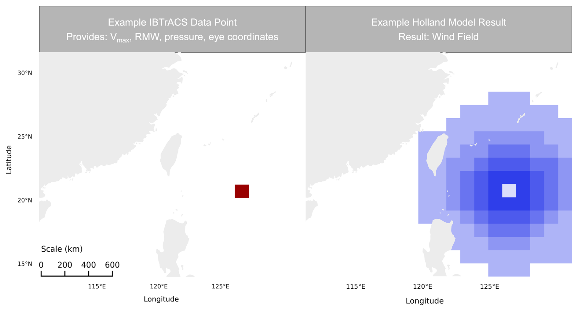
Figure 3 Illustration depicting an example data point from the IBTrACS dataset and the wind field result from using the parameters from the data point as an input into the Holland model.

2.5 Height scaling for wind

The Holland model outputs wind speed at gradient level (Holland, 1980), the height at which surface friction no longer significantly affects the wind flow. Therefore, the wind speed needs to be scaled to a height that is of use. For this paper, the wind speed has been scaled to 100 m. Franklin et al. (2003) suggest that, for TCs, the layer below the broad maximum wind speed of 500 m, approximately follows the logarithm of the altitude. To scale the wind, firstly, the geostrophic drag law is solved for the friction velocity (Rossby and Montgomery, 1935; Blackadar and Tennekes, 1968):

$$\begin{array}{}\text{(3)}& \text{G}={\displaystyle \frac{u_{*}}{\mathit{\kappa }}}\sqrt{{\left(\ln \left({\displaystyle \frac{u_{*}}{f_{\text{col}}\cdot z_{\mathrm{0}}}}\right)-A\right)}^{\mathrm{2}}+C^{\mathrm{2}}},\end{array}$$

where u_* is the friction velocity, G is the geostrophic wind, κ is the con Kármán constant, f_col is the Coriolis parameter, z₀ is the surface correction parameter, and A and C are constants defined by the neutral conditions. The constants are set as A=1.8 and C=4.5. Using the friction velocity, the wind speed is scaled to a different height using the logarithmic wind law

$$\begin{array}{}\text{(4)}& u\left(z\right)={\displaystyle \frac{u_{*}}{\mathit{\kappa }}}\ln {\displaystyle \frac{z}{z_{\mathrm{0}}}},\end{array}$$

where z is the target height. Combining the geostrophic wind law with the logarithmic profile of the wind is a well-established method and already implemented into systems such as the Wind Atlas Analysis and Application Program (WAsP) (Troen and Petersen, 1989).

The wind speeds were originally scaled to 10 m for comparison against the IBTrACS dataset. The approach was performed for varying surface correction parameters for each region. The optimal surface correction parameter was selected by evaluating, on average, how well the scaled wind speeds match the 10 m IBTrACS data. The adjusted values for the surface correction parameter identified are 5e⁻⁶, 9e⁻⁶, and 1e⁻⁵ m for the Taiwan, Japan, and ECUS regions, respectively. Note that although the roughness length would usually be used, here a surface correction parameter is used in its place. The rationale for this approach is discussed in detail in Appendix A.

The commonly accepted deep ocean surface roughness value is 0.2 mm (He et al., 2021). However, Ott (2006) shows that the eyewall profile follows the logarithm of the altitude using a surface roughness of 0.07 mm.

To scale to 100 m, the same method was performed using the adjusted roughness length.

2.6 The Gumbel distribution

For each individual grid point and for each year, the maximum wind speed at 100 m is obtained following Sect. 2.4 and 2.5. Using the annual maxima, the Gumbel distribution estimates U₅₀. This method follows the approach described in Abild (1994) and Larsén et al. (2015), in which X_m is the ascending sorted annual maxima (for each grid point), with n samples.

The sample mean is computed as

$$\begin{array}{}\text{(5)}& b_{\mathrm{0}}={\displaystyle \frac{\mathrm{1}}{n}}\sum _{i=\mathrm{1}}^n{X}_{\mathrm{m},i}\end{array}$$

and the weighted mean

$$\begin{array}{}\text{(6)}& b_{\mathrm{1}}={\displaystyle \frac{\mathrm{1}}{(n-\mathrm{1})n}}\sum _{i=\mathrm{1}}^n(i-\mathrm{1})\cdot X_{\mathrm{m},i}.\end{array}$$

The Gumbel distribution parameters α and β can be calculated such that

$$\begin{array}{}\text{(7)}& \mathit{\alpha }={\displaystyle \frac{\ln \mathrm{2}}{\mathrm{2}{b}_{\mathrm{1}}-b_{\mathrm{0}}}}\text{ and }\mathit{\beta }=b_{\mathrm{0}}-{\displaystyle \frac{\mathit{\gamma }}{\mathit{\alpha }}},\end{array}$$

where γ is Euler's constant = 0.57721. The wind speed for the return period T is

$$\begin{array}{}\text{(8)}& U_T=-{\displaystyle \frac{\mathrm{1}}{\mathit{\alpha }}}\ln \left(\ln \left({\displaystyle \frac{T}{T-\mathrm{1}}}\right)\right)+\mathit{\beta },\end{array}$$

and the standard deviation associated with the wind speed for the return period T is

$$\begin{array}{}\text{(9)}& {\mathit{\sigma }}_T={\displaystyle \frac{\mathit{\pi }}{\mathit{\alpha }\sqrt{\mathrm{6}n}}}\sqrt{\mathrm{1}+\mathrm{1.14}{k}_T+\mathrm{1.1}{k}_T^{\mathrm{2}}},\end{array}$$

where $k_T=\frac{\sqrt{\mathrm{6}}}{\mathit{\pi }}\left(-\ln \left(\ln \left(\frac{T_{\text{return}}}{T_{\text{return}}-\mathrm{1}}\right)\right)-\mathrm{0.577}\right)$.

Using the yearly maximum for the Gumbel fit can result in the discarding of other large storms that occur in the same active year. This, in turn, could lead to the tail retaining less information than other approaches. Since U₅₀ is derived in the Gumbel distribution by extrapolating the fitted tail to an exceedance probability, the estimate could carry additional uncertainty. A peak-over-threshold approach using the generalised Pareto distribution was tested, but the grid resolution produced too few exceedances per point. This led to unstable and often negative shape parameters. The Gumbel distribution remains a standard choice, but for this procedure, the resulting U₅₀ represents the wind level associated with exceedance of the yearly maximum, rather than the full set of extreme storms that may occur within a year.

3 Results

The results of calculating U₅₀ are presented in three regions: the Taiwan, Japan, and ECUS regions shown here. Each region will be discussed individually.

3.1 Taiwan

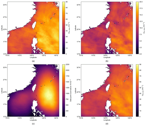
In Fig. 4a, U₅₀ at 100 m is presented for the Taiwan region. The region expands from latitude 12 to 33.5° N and longitude 110 to 131.5° E. Taiwan is located in the centre of the figure, with the Philippines to the south and mainland China to the west.

The highest values of U₅₀ are observed east of longitude 120° E, corresponding to areas east of Taiwan and the Philippines. In contrast, in the west of Taiwan and the Philippines, the wind speed is slower by approximately 10–20 m s⁻¹. The majority of TCs forming in the western Pacific form to the south-east of Taiwan (Guo et al., 2025), where they can intensify before weakening as they approach or move over land (Park et al., 2013). Therefore, it is expected to see the highest winds south-east of Taiwan, before reaching land. The spatial distribution of the wind field looks somewhat consistent with previous studies based on IBTrACS data, such as Ott (2006) and Kong et al. (2024). To compare with the results of Ott (2006) and Kong et al. (2024), U₅₀ at 10 m is also provided here (Fig. 4d). The maximum value of U₅₀ at 10 m in this area is 72.7 m s⁻¹, which is 72 m s⁻¹ in Ott (2006) and 70.4 m s⁻¹ in Kong et al. (2024). Figure 4d here also includes more detailed spatial variability of U₅₀ at 10 m than Ott (2006) and Kong et al. (2024) due to their larger spatial grid spacing of 1° × 1°. It should be noted that the spatial distribution of Fig. 4a and d is very similar, and the 10 m results simply return smaller values. The detailed spatial distribution of U₅₀ at 100 m in this study is similar to the results in Larsén and Ott (2022) (their Fig. 7a), which was based on the CFSR reanalysis data with grid spacing of about 40 km, where the values of U₅₀ were corrected to an equivalent temporal resolution of 10 min. While Imberger et al. (2024) present results at 50 and 150 m using CFSR, MERRA 2, and ERA5, the resultant dataset from the project has also been made available. Examining the 100 m results, the spatial distribution appears most similar to the CFSR output, with the peak located to the east of the Philippines. Meanwhile, for the ERA5 and MERRA 2 results, the peak is located further north. The maximum U₅₀ at 100 m in this analysis is 84.3 m s⁻¹, which is closest to the ERA5 estimate of U₅₀ of 86.7 m s⁻¹.

The 95 % confidence interval calculated using Eq. (9) in connection with the use of Gumbel distribution is shown in Fig. 4b. It widens in areas where U₅₀ increases, peaking at approximately 15 m s⁻¹, and it narrows to approximately 2 m s⁻¹ at the smallest. In this context, the 95 % confidence interval reflects the variability associated with the fitted Gumbel distribution. It does not represent the uncertainty of all input parameters. Uncertainties relating to the entire process are discussed in Sect. 4. Given that the Holland model is applied to every IBTrACS data point that fits the criteria, all grid points have the same number of data points, which are listed in Table 2. To illustrate which areas in each region contain the highest wind speeds, Fig. 4c has been developed. It shows the number of data points above 19 m s⁻¹ from the Holland model at each grid point. NOAA defines a tropical storm when the 1 min average winds reach 34 kt at 10 m. By converting 34 kt to m s⁻¹, a 10 min average, and scaling the wind speed height to 100 m, the threshold becomes 19 m s⁻¹. These methods are all described in Sect. 2. The same reasoning holds true in Sect. 3.2 and 3.3.

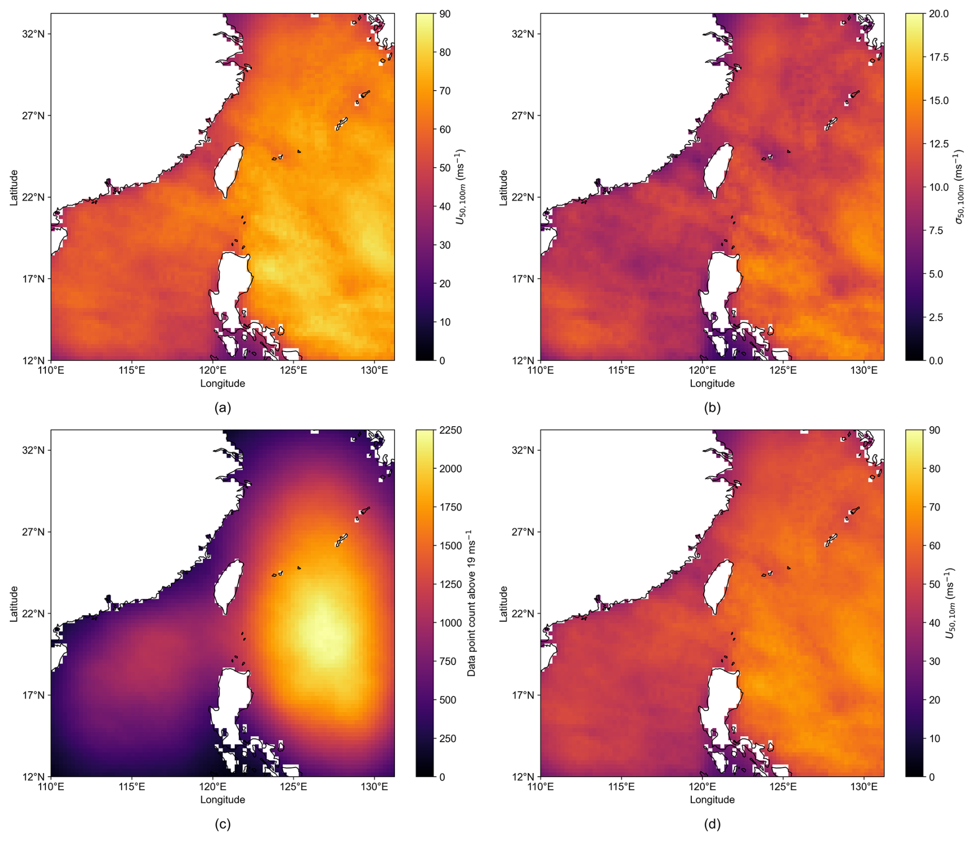
Figure 4 Results for Taiwan. (a) U₅₀ at 100 m. (b) The 95 % confidence interval from the Gumbel distribution calculated using 1.96σ₅₀. (c) The number of data points from the Holland model calculation that are equal to or above 19 m s⁻¹. (d) U₅₀ at 10 m.

3.2 Japan

In Fig. 5a, U₅₀ at 100 m is presented for the Japan region. The region expands from latitude 21 to 55.5° N and longitude 120.6 to 156° E. Japan is located in the centre of the figure, with South Korea, North Korea, Russia, and China located to the west. In this region, the genesis of TCs typically occurs at lower latitudes, and they move in a north-west direction. The Coriolis force turns the TCs farther north, and once it has reached mid-latitudes, the TC turns eastward due to westerlies in addition to the Coriolis force (Cao et al., 2025). As they move north, the sea water temperature typically becomes cooler and the TC weakens (Fei et al., 2020), hence the higher U₅₀ values occurring at latitudes lower than 36° N while the TC still holds intensity. In Fig. 5c, showing the number of values each grid point has above 19 m s⁻¹, there are far fewer data points above 36° N latitude in comparison to below 36° N latitude, and above 46° N latitude, there are few to no data points giving an explanation as to why wind speeds approach 0 m s⁻¹ in this region. However, this does not mean that the extreme wind speed in these areas is negligible, as other weather processes can take place, but this study solely focuses on tropical cyclone extreme wind speed. This clearly demonstrates the uncertainty associated with too few data samples.

The southern coastline of Japan is the most exposed, although both the south-western and south-eastern coastlines still experience elevated wind speeds due to TCs. As in the Taiwan region, the 95 % confidence interval increases with wind speed, reaching its highest values in areas where there is substantial and strong TC activity.

The spatial distribution as well as the magnitude of U₅₀ at 100 m in Fig. 5a is quite similar to that in Larsén and Ott (2022) (their Fig. 7a) for the overlapping area, including the patchy patterns. Such levels of detail are absent in Ott (2006) and Kong et al. (2024) due to the coarser spatial resolution. The results presented here differ spatially from Imberger et al. (2024). In Imberger et al. (2024), peak wind speeds occur primarily below 35° N and up to 140° E, with a north-eastward trailing feature. In contrast, this analysis shows a less pronounced decrease beyond 140° E and does not capture this north-eastward feature. This could be due to the difference in sample size at high latitudes, as the dataset used in Imberger et al. (2024) does not exhibit the same reduction in data availability with increasing latitude. The maximum U₅₀ in this study is lower than all values used in Imberger et al. (2024); however, the ERA5 and MERRA 2 maxima are shifted farther north into the Japan region, where as the CFSR results are more consistent with those presented here, aside from a single pronounced peak in the Imberger et al. (2024) analysis.

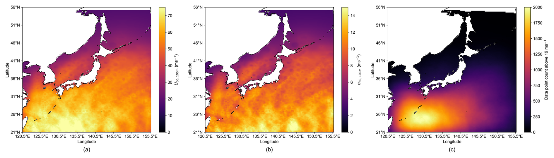
Figure 5 Results for Japan. (a) U₅₀ at 100 m. (b) The 95 % confidence interval from the Gumbel distribution, calculated using 1.96σ₅₀. (c) The number of data points from the Holland model calculation that are equal to or above 19 m s⁻¹.

3.3 East coast of the US

In Fig. 6a, U₅₀ at 100 m is presented for the ECUS region. The region expands from latitude 22 to 57.5° N and longitude 88.5 to 57° W. The east coast of the US is shown, along with the top of the Caribbean in the south.

The results from the ECUS region deviate from expectations. At a granular scale, the eyewall of the TC is evident as it traverses over the region, and the U₅₀ field exhibits a fragmented structure, which is discussed in Sect. 5. On a macro scale, the spatial distribution of U₅₀ maxima and minima is unexpected. The highest wind speeds were anticipated to occur consistently in the lower half of the region. This distribution was expected due to the positive correlation between latitude and RMW (Kimball and Mulekar, 2004; Vickery and Wadhera, 2008; Pérez-Alarcón et al., 2021), and TCs in the Gulf of Mexico, on average, have a smaller RMW than those in the Atlantic (Vickery and Wadhera, 2008). The intensity of a TC is inversely related to the RMW (Kimball and Mulekar, 2004; Chavas and Knaff, 2022), meaning that, on average, storms with smaller RMW tend to have stronger winds than TCs with large RMW.

The results here show that while the highest return level is 74.9 m s⁻¹ at 26.75° N latitude and 64.75° W longitude, the latitude farther north also exhibits return levels which are nearly as high. The wind speeds between latitudes 33 and 40° N, and longitudes 64.5 and 59.5° W are noted as rather high.

The 95 % confidence intervals follow the same pattern as in the previous cases: regions with higher wind speeds correspond to a widening confidence interval. Furthermore, the confidence interval structure also follows the same structure as U₅₀.

The study of Larsén and Ott (2022), reflecting the reanalysis CFSR wind field, does suggest a stronger U_50,100 m band south of 30° N, between about 30° N, 75° W and 22° N, 65° W, with the highest value of about 73 m s⁻¹. Due to the Coriolis force and westerlies, this strong U_50,100 m band turns north-east (their Fig. 7c). Compared to Larsén and Ott (2022), Fig. 6b here captures the second, relatively weaker extreme wind band north of 30° N and did not capture the full picture of the first, stronger extreme wind band. We argue that it is, on one side, caused by the few IBTrACS tracks in this region (see Fig. 6c), and on the other side, related to the application of the Holland model. A detailed discussion is provided in Sect. 5. The hotspot in the Caribbean is both present in the current study and in Larsén and Ott (2022). Imberger et al. (2024) identify a Caribbean hotspot across all three datasets. In addition, the CFSR results show a separate, lower-latitude hotspot in the Atlantic Ocean that is not evident in the ERA5 or MERRA 2 outputs, which this analysis is more inline with. The CFSR and MERRA 2 datasets otherwise place their primary peaks above 35° N. The maximum wind speed in this analysis (74.9 m s⁻¹) is closest in magnitude to the CFSR value of 72.0 m s⁻¹, although the locations of these maxima differ substantially.

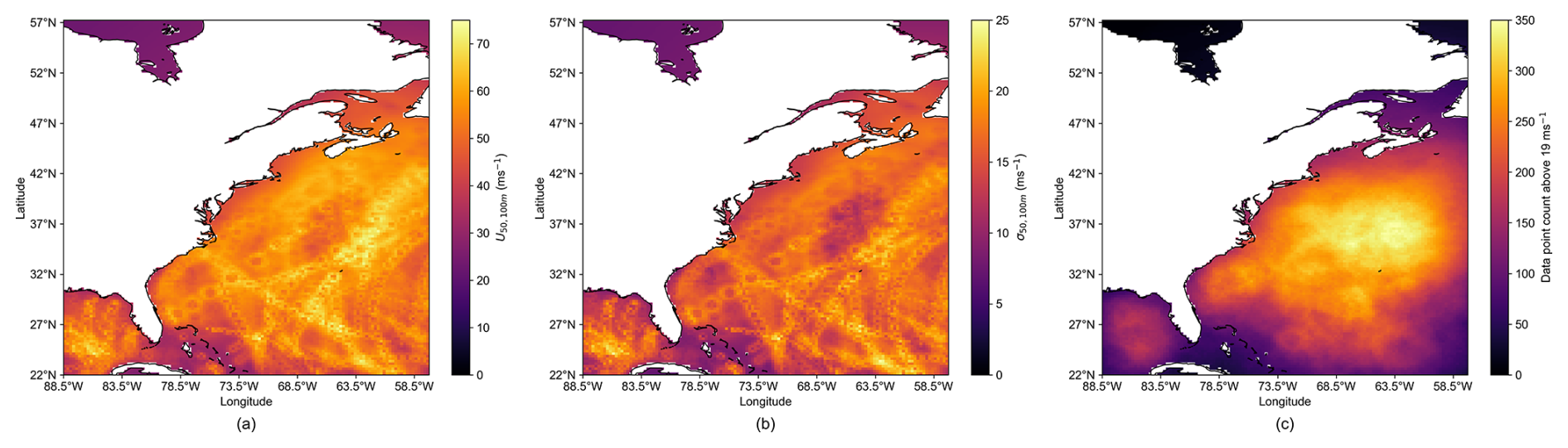
Figure 6 Results for ECUS. (a) U₅₀ at 100 m. (b) The 95 % confidence interval from the Gumbel distribution, calculated using 1.96σ₅₀. (c) The number of data points from the Holland model calculation that are equal to or above 19 m s⁻¹.

4 Uncertainty analysis

As outlined in Sect. 2, there are several input parameters into the Holland model and the Gumbel distribution, which could introduce uncertainty into the estimation of U₅₀. Given the number of contributing variables, a Monte Carlo (Metropolis and Ulam, 1949) approach was used to propagate uncertainty throughout the method. The parameters considered include wind speed, centre position, RMW, pressure, the B parameter, and scaled wind speed. Monte Carlo simulations are a common method to estimate uncertainty in the wind energy sector, as shown by Ishihara and Yamaguchi (2015), Yasui et al. (2002), and Hu et al. (2023)

Most parameters in the uncertainty analysis are sourced from the IBTrACS dataset, and while data from many agencies are consolidated, the associated errors are not, making the quantification of uncertainty challenging. IBTrACS is typically used as a reference dataset for validation purposes and does not consistently report uncertainty estimates for all variables. Therefore, bespoke methods to quantify each parameter's uncertainty have been used. Some parameters have a uniform range defined; others require a comparison of values from various agencies for a standard deviation to be calculated; and one requires error propagation.

The uncertainty associated with the sampling rate of IBTrACS is not quantified in this section. The dataset provides 3-hourly observations, and no interpolation to a finer resolution was performed to avoid introducing additional uncertainty. The aim is to evaluate the method using the raw IBTrACS data. A second source of uncertainty that has not been extensively evaluated is the climatological variability of the underlying dataset. An attempt was made to quantify this by splitting each regional dataset into two equal halves and fitting the Gumbel distribution independently to each half. The difference between the two half-period estimates was tested for statistical significance by identifying differences between the two results that fell outside of the combined Gumbel confidence interval. Almost no grid points showed a statistically significant difference between the two periods. This indicates that the Gumbel uncertainty dominates over any detectable shift in the extreme wind climate between the two halves.

Here in the Monte Carlo framework, each parameter was randomly sampled with an estimated 95 % confidence interval using ±1.96σ, allowing comparisons across parameters. The method was repeated 100 times for each parameter. The following section outlines the approach taken to estimate the uncertainty for each variable.

4.1 Uncertainty associated with key parameters

4.1.1 Wind speed

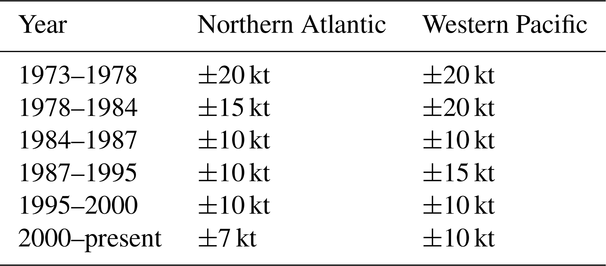
Wind speed is one of the few parameters for which uncertainties are provided in the IBTrACS documentation (IBTrACS Science Team, 2025), shown in Table 5. As noted by the IBTrACS documentation, the uncertainty estimates are calculated from the contributions from the third IBTrACS Workshop attendees. It takes into account the changes of forecasting methods over the year, changes in aircraft reconnaissance in the western Pacific and northern Atlantic, and information provided from more than one agency for several basins. The absolute uncertainties change based on both year and ocean basin, and are noted to be qualitative in nature.

While the absolute uncertainty is uniformly distributed, for this paper, the error distribution has been approximated as Gaussian, with the half-width a being equivalent to 1.96σ. Note that while the IEC standard outlines that parameters such as wind speed may follow a Weibull distribution, the present analysis assumes a Gaussian for the associated error rather than the parameter itself. This is a further step of approximation than that from BIPM and IEC and IFCC and ILAC and ISO and IUPAC and IUPAP and OIML (2008), which estimates the standard deviation of a uniform distribution as

$$\begin{array}{}\text{(10)}& \mathit{\sigma }={\displaystyle \frac{a}{\sqrt{\mathrm{3}}}}.\end{array}$$

For all parameters for which the absolute uncertainty is provided, the same approximation will take place.

Table 5 IBTrACS wind speed uncertainty (knots).

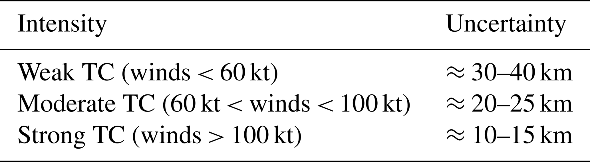
4.1.2 Position

The position refers to the centre latitude–longitude location of a TC. The uncertainty for the position is also available from the IBTrACS documentation and is shown in Table 6. Following the approximation in Sect. 4.1.1, the upper range of the absolute uncertainty is approximated as 1.96σ, for example, 1.96σ=40 km; therefore the latitude and longitude will be varied within ±40 km from their original position.

Table 6 IBTrACS position uncertainty (kilometres).

4.1.3 RMW

The RMW uncertainty has been calculated differently for the northern Atlantic, where ECUS lies, and the western Pacific, where the Taiwan and Japan regions lie.

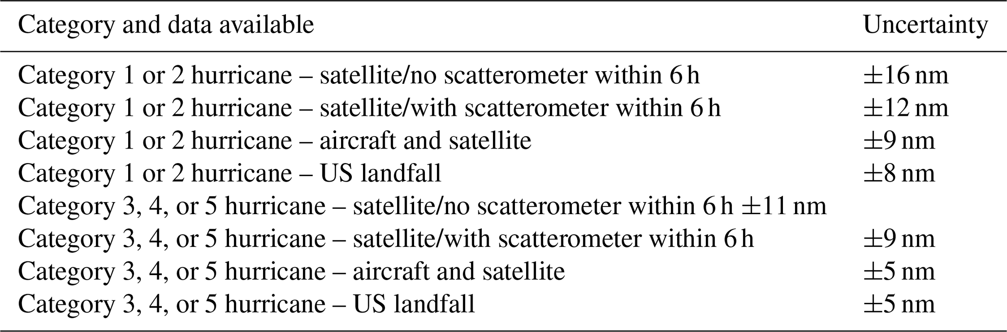
The ECUS region will first be discussed. The US agencies' RMW uncertainty can be found in an online NOAA report at https://www.nhc.noaa.gov/data/hurdat/hurdat2-format-atl-1851-2021.pdf (last access: 15 September 2025), and a subset is shown in Table 7. The report details extra information on the HURDAT2 dataset (Landsea and Franklin, 2013), which is supplied to IBTrACS.

For the ECUS region, only the years from 2001 are included. Satellites carrying scatterometers were active for the entire period of analysis. Satellites providing near-global ocean coverage every 1–2 d include QuikSCAT (1999–2009) (Hoffman and Leidner, 2005), ASCAT on MetOp-A (from 2006) (Figa-Saldaña et al., 2002; Wagner et al., 2013), and MetOp-B/C (from 2012/2018) (Wagner et al., 2013). Regions in which TCs occur are a priority for satellite coverage as many agencies rely on up-to-date coverage of TCs for modelling and accurate short-term forecasts (Kishtawal, 2016). Therefore, the absolute uncertainty was selected to be 12 nautical miles (approximately 22 km).

Given the approximation in Sect. 4.1.1, we define the absolute uncertainty, 12 nm equivalent to 1.96σ, and vary the RMW within this range.

Table 7 US agencies IBTrACS radius of maximum wind uncertainty (nautical miles).

For the Western Pacific, the outcome of converting the 50 km radius to the RMW is compared to available values from the US agencies in the western Pacific region. From the differences, the mean standard deviation was 10567 m.

4.1.4 Pressure

For the northern Atlantic, Landsea and Franklin (2013) define the absolute pressure uncertainty as 9.5 hPa for major TCs observed via satellite. For weaker TCs, such as category 1 or 2, the uncertainty is smaller. Therefore, using the uncertainty of 9.5 hPa is likely a conservative approach. Following the approximation in Sect. 4.1.1, we assign the absolute uncertainty (9.5 hPa) as equivalent to 1.96σ and vary the pressure value within this range.

In the western Pacific, multiple agencies provide pressure values for the same TC time steps. These agencies include the JMA, HKO, CMA, and US. Pressure values from these various agencies for each TC and time step were compared against each other. The comparisons were used to calculate the mean standard deviation, which returned as 2.13 hPa and set as equivalent to 1.96σ.

4.1.5 B parameter

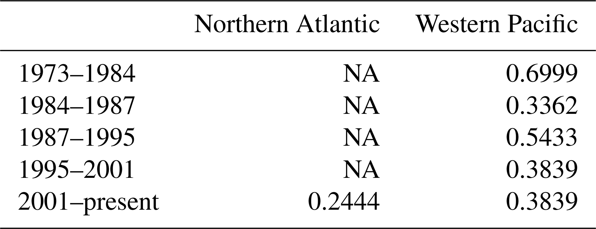
The B parameter is not provided directly in the IBTrACS dataset but rather calculated from other variables. These variables are the central pressure and the maximum wind speed. As a result, there is no documented uncertainty associated with the B parameter. To estimate its uncertainty, the error propagation formula for correlated variables is applied:

$$\begin{array}{}\text{(11)}& \begin{array}{rl}{\mathit{\sigma }}_b^{\mathrm{2}}& ={\left({\displaystyle \frac{\partial b}{\partial V_{\text{max}}}}\right)}^{\mathrm{2}}{\mathit{\sigma }}_{V_{\text{max}}}^{\mathrm{2}}+{\left({\displaystyle \frac{\partial b}{\partial P_c}}\right)}^{\mathrm{2}}{\mathit{\sigma }}_{P_c}^{\mathrm{2}}\\ & +\mathrm{2}\left({\displaystyle \frac{\partial b}{\partial V_{\text{max}}}}\right)\left({\displaystyle \frac{\partial b}{\partial P_c}}\right)\text{Cov}(V_{\text{max}},P_c).\end{array}\end{array}$$

This expression is derived from the first-order Taylor expansion, and its general application is described in Taylor (1997), while its application to meteorological contexts is described in detail in BIPM and IEC and IFCC and ILAC and ISO and IUPAC and IUPAP and OIML (2008).

The estimation relies on the assumption that the errors are small compared to the mean of the maximum wind speed and the pressure, the errors are unbiased and symmetric, and the errors are independent or the covariance is accounted for, which is the case here.

In the western Pacific, the uncertainty in wind speed varies over time, resulting in corresponding temporal variation in the B parameter uncertainty. Once the variation in wind speed uncertainty over time is taken into account, for each time period, the mean B parameter standard deviation is found and used. In contrast, for ECUS, only data from 2001 onward are used, during which a single wind speed uncertainty value applies. Consequently, a single B parameter uncertainty estimate is reported for the ECUS region.

Table 8 B parameter standard deviation (unitless). NA: not available.

4.1.6 Scaled wind speed

The Holland model returns the wind speed at the gradient level. To understand the wind speed impact on offshore infrastructure, the wind speed at a more relevant height should be calculated. The method of scaling the wind height from the gradient level to 100 m is detailed in Sect. 2.5. For validation, the wind speed was scaled to 10 m and the value was compared against IBTrACS. Using the difference between the two, the standard deviation could be calculated.

Table 9 Scaled wind speed standard deviation (m s⁻¹).

4.1.7 Contributions to total uncertainty

To assess the influence of input parameters on the overall uncertainty of U₅₀, a variance-based sensitivity analysis is performed. This captures both individual effects and interaction terms. This approach is an approximation of the first and second order indices of Sobol (2001). Sobol's indices are widely used in sensitivity analysis (Dykes et al., 2014; Locatelli et al., 2017; Thapa and Missoum, 2022; Tsvetkova and Ouarda, 2019). However, this implementation follows a simpler approach: parameters are randomly sampled in their 95 % confidence intervals. Let $x_{p,m,i}$ be the value of parameter p of Monte Carlo simulation m at grid point i. Normalise each value at each grid point for each parameter:

$$\begin{array}{}\text{(12)}& {\stackrel{\mathrm{̃}}{x}}_{p,m,i}={\displaystyle \frac{x_{p,m,i}-{\stackrel{\mathrm{‾}}{x}}_{p,i}}{{\stackrel{\mathrm{‾}}{x}}_{p,i}}},\end{array}$$

where ${\stackrel{\mathrm{̃}}{x}}_{p,i}$ is the mean of all simulation values for grid point i and parameter p. First, the variation around the mean is calculated using $x_{p,m,i}-{\stackrel{\mathrm{‾}}{x}}_{p,i}$. Following this, the variation is normalised by ${\stackrel{\mathrm{‾}}{x}}_{p,i}$ to find the relative variation. The relative variation is used so that a direct comparison can be made between parameters that have different units and scales of magnitude.

To calculate the variance (diagonal terms), which represents the individual parameters' contributions to total uncertainty, the following steps are taken. First, the variance term of parameter p at a singular grid point i is calculated by

$$\begin{array}{}\text{(13)}& {\text{Var}}_{p,i}={\displaystyle \frac{\mathrm{1}}{N}}\sum _{\mathrm{m}}{\stackrel{\mathrm{̃}}{x}}_{p,m,i}^{\mathrm{2}},\end{array}$$

where N is the total number of simulations. The total variance from all parameters is defined as

$$\begin{array}{}\text{(14)}& {\text{Var}}_{\text{diag total}}=\sum _{p,i}{\text{Var}}_{p,i}.\end{array}$$

To account for the interaction terms, the covariance is computed, showing how parameter uncertainties interact. A positive value indicates that the parameters amplify each other's uncertainty, whereas a negative value indicates that the parameters partially counteract each other's uncertainty. The magnitude of the value indicates how strong this interaction is and how much the interaction contributes to the overall uncertainty. While each Monte Carlo simulation varies a singular parameter at each time, following the completion of the simulations, ${\stackrel{\mathrm{̃}}{x}}_{p,m,i}$ can be calculated for each parameter at each grid point. This allows the calculation of the covariance term between parameters p₁ and p₂ at a singular grid point i and can be shown as

$$\begin{array}{}\text{(15)}& {\text{Cov}}_{p_{\mathrm{1}},p_{\mathrm{2}},i}=\mathrm{2}{\displaystyle \frac{\mathrm{1}}{N}}\sum _{\mathrm{m}}{\stackrel{\mathrm{̃}}{x}}_{p_{\mathrm{1}},m,i}{\stackrel{\mathrm{̃}}{x}}_{p_{\mathrm{2}},m,i},\end{array}$$

where N is the total number of simulations. The contribution to the total off-diagonal variance from the covariance terms sum over all possible combinations:

$$\begin{array}{}\text{(16)}& {\text{Var}}_{\text{off-diag total}}=\sum _{\begin{array}{c}x,y\\ x\ne y\end{array}}\sum _i{\text{Cov}}_{p_x,p_y,i},\end{array}$$

where x≠y ensures that only distinct pairs of parameters are considered at each grid point.

The total variance can be defined as the sum of all variance and covariance terms and is 100 %.

$$\begin{array}{}\text{(17)}& {\text{Var}}_{\text{total}}={\text{Var}}_{\text{diag total}}+{\text{Var}}_{\text{off-diag total}}\end{array}$$

To calculate the percentage of total variation that each individual parameter and each interaction contributes towards is calculated by summing the variation for each individual parameter and each interaction across all grid points:

$$\begin{array}{}\text{(18)}& {\displaystyle }{\text{Var}}_p=\sum _i{\text{Var}}_{p,i}\text{(19)}& {\displaystyle }{\text{Var}}_{p_x,p_y}=\sum _i{\text{Cov}}_{p_x,p_y,i},\end{array}$$

and dividing by the total variation from all parameters and interactions calculated in Eq. (17).

4.2 Uncertainty results

The mean U₅₀ and the standard deviation were calculated for each parameter for each set of 100 simulations. Each parameter was varied exclusively, while all others were held constant. Each parameter was varied within its approximate 95 % confidence interval. The regional results are presented in Figs. 7, 8 and 9.

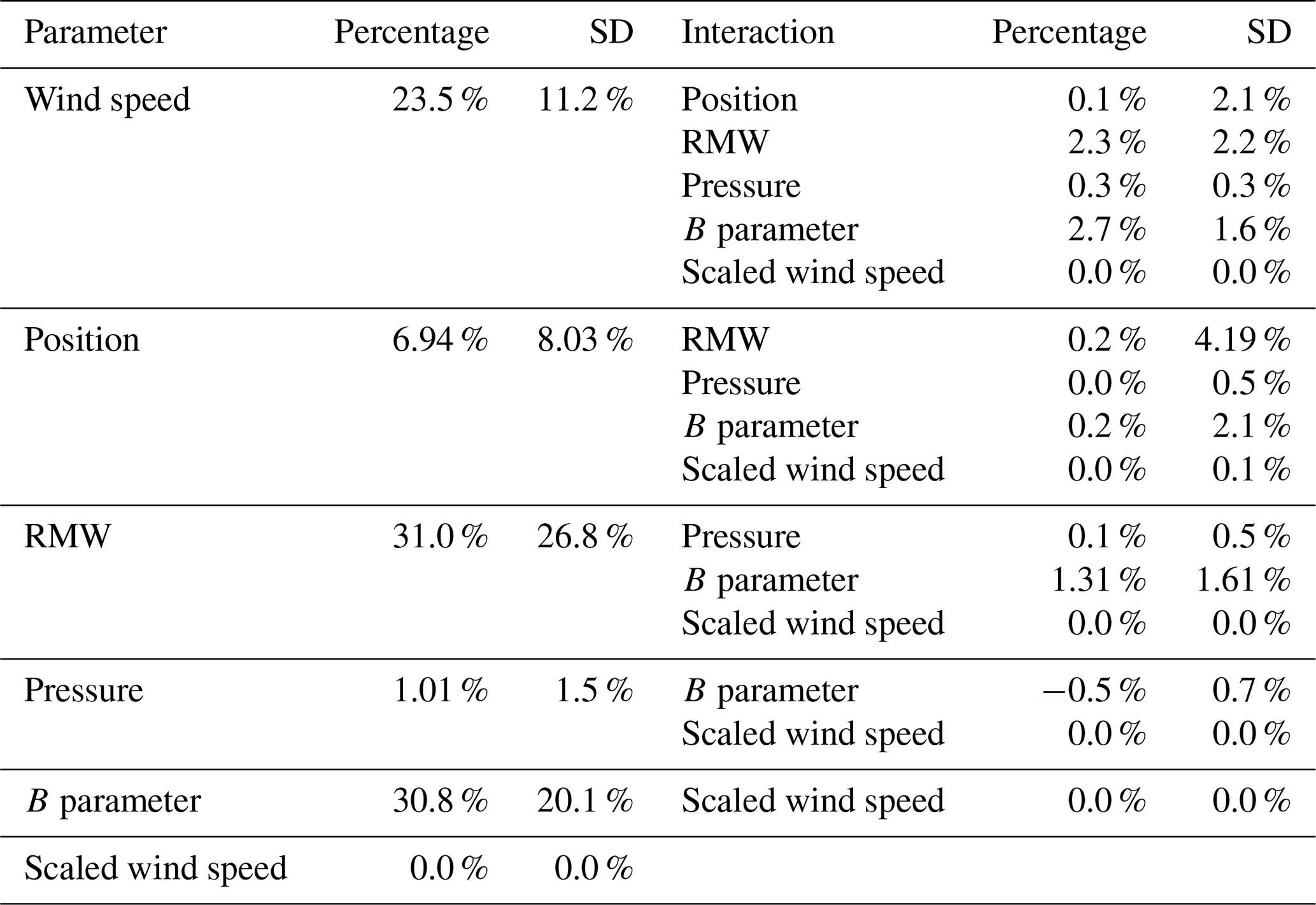
As shown in Tables 10, 11, and 12, across all regions, specific individual parameters dominate the overall uncertainty, rather than the interactions, where all parameter interactions contribute below 1 % in all cases.

The results shown in Tables 10 for Taiwan and 11 for Japan are, as expected, similar. They are in close proximity and have similar data restrictions. In both regions, the B parameter dominates the impact on the overall uncertainty. This could be attributed to the B parameter incorporating the uncertainty of two parameters, leading to a larger combined variance. The RMW has a smaller impact on the Taiwan and Japan regions; however, it contributes significantly to uncertainty in the ECUS region, particularly to the south, which is further discussed in Sect. 5. In the ECUS region, RMW, wind speed, and the B parameter have similar uncertainty; however, the method takes into account the entire defined region. From Fig. 9, it is clear that the RMW uncertainty is primarily heightened in the southern half of the region. By breaking the region down further, the contribution to overall uncertainty would likely shift.

Wind speed uncertainty for all regions has a substantial impact, which is expected given its direct role in the U₅₀ calculation. Surprisingly, pressure uncertainty shows little influence in all three regions, suggesting that either the Holland model has low sensitivity to pressure variation or that the uncertainty associated with pressure is minimal. Scaling the wind speed and changing the latitude/longitude of the maximum wind speed appear to have a negligible impact on the overall uncertainty.

Examining the interaction contributions to the total uncertainty in Tables 10, 11, and 12, given that RMW, wind speed, and the B parameter are the biggest individual contributors to uncertainty, it is unsurprising that their interactions are the biggest contributions to uncertainty. Two notable features of the data are observed: (1) the largest interaction is between the RMW and B parameter in Taiwan, accounting for 7.2 %; (2) the wind speed–B parameter interaction in Japan is negative, indicating that the uncertainty of these parameters partially counteract each other. However, given the confidence intervals associated with all interaction contributions, these effects could be close to negligible. Therefore, the primary focus should remain on the individual effects.

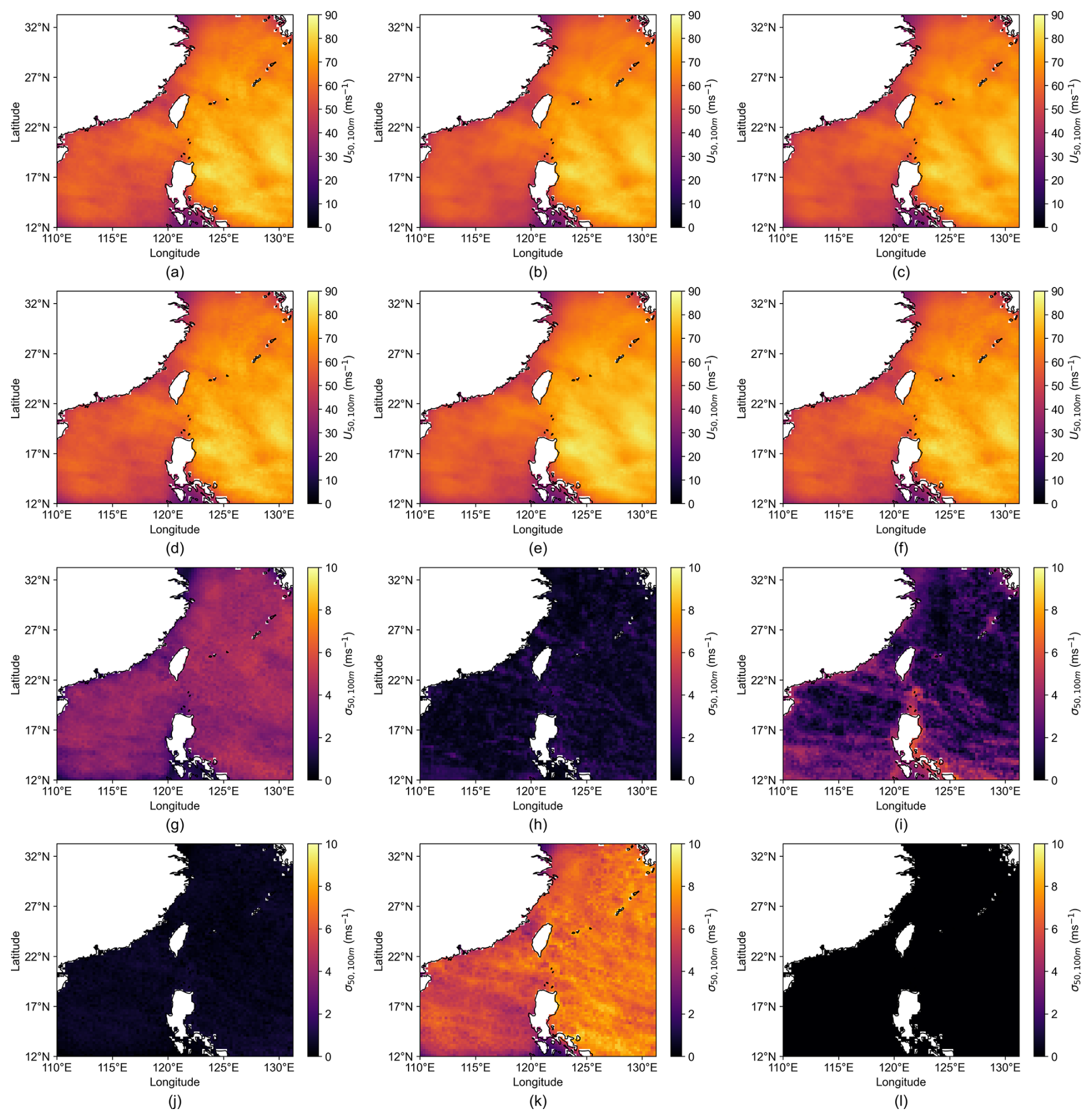
Figure 7 Monte Carlo simulation results for Taiwan. (a)–(f) show the mean wind speed from 100 simulations for each varying parameter, and (g)–(l) show the standard deviation from 100 simulations for each varying parameter. (a) and (g) wind speed. (b) and (h) eye coordinates. (c) and (i) RMW. (d) and (j) pressure. (e) and (k) B parameter. (f) and (l) scaled wind speed.

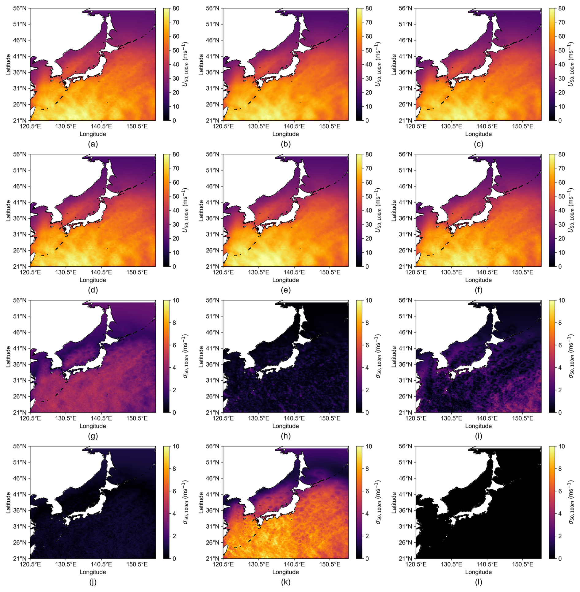
Figure 8 Monte Carlo simulation results for Japan. (a)–(f) show the mean wind speed from 100 simulations for each varying parameter, and (g)–(l) show the standard deviation from 100 simulations for each varying parameter. (a) and (g) wind speed. (b) and (h) eye coordinates. (c) and (i) RMW. (d) and (j) pressure. (e) and (k) B parameter. (f) and (l) scaled wind speed.

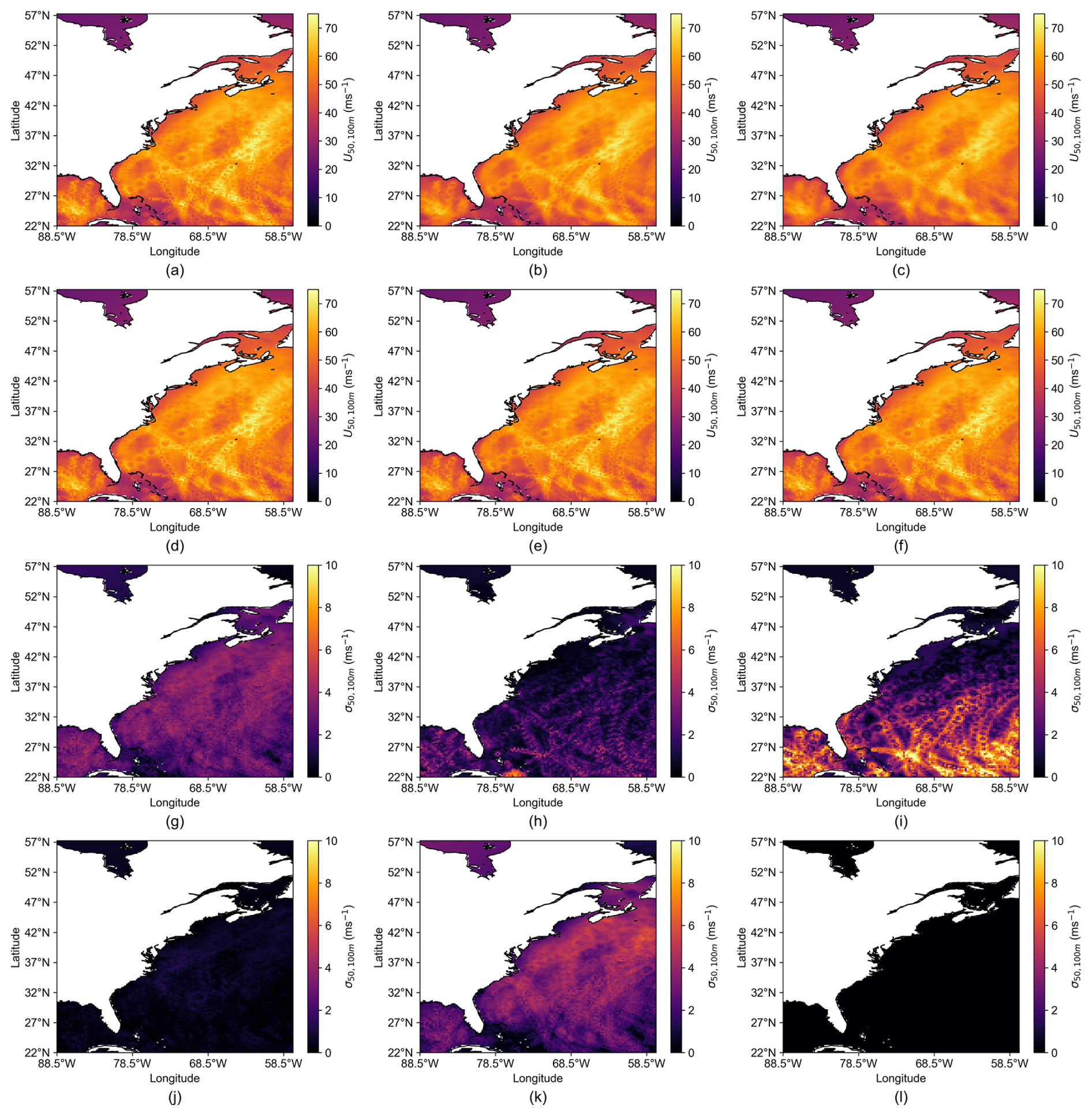
Figure 9 Monte Carlo simulation results for ECUS. (a)–(f) show the mean wind speed from 100 simulations for each varying parameter, and (g)–(l) show the standard deviation from 100 simulations for each varying parameter. (a) and (g) wind speed. (b) and (h) eye coordinates. (c) and (i) RMW. (d) and (j) pressure. (e) and (k) B parameter. (f) and (l) scaled wind speed.

Table 10 Contribution to total uncertainty in Taiwan (percentage).

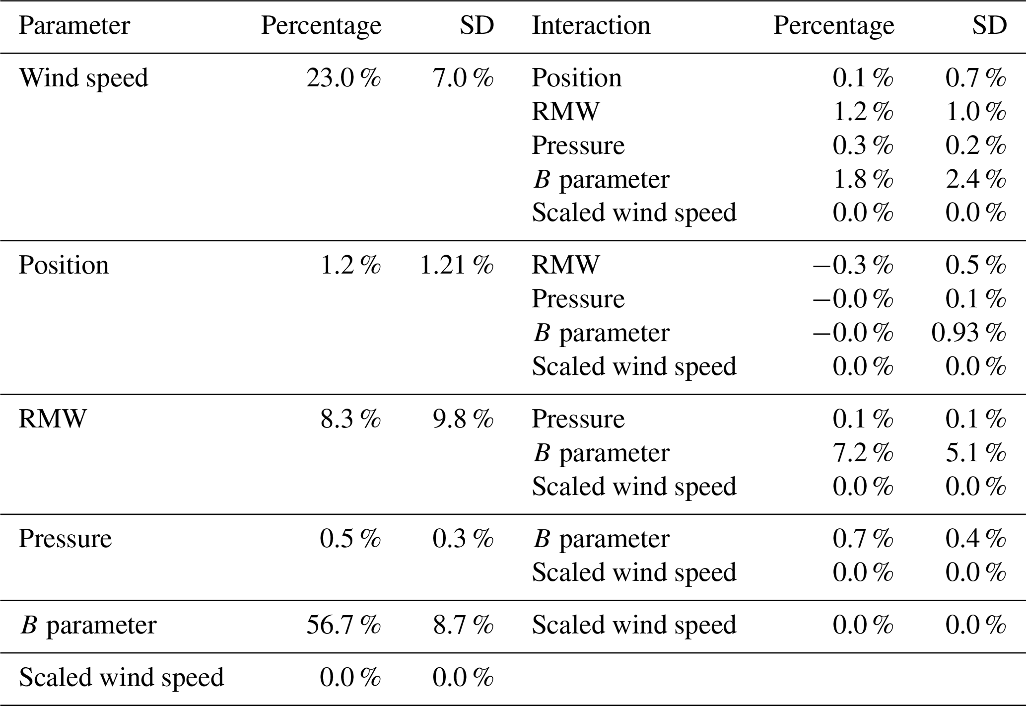
Table 11 Contribution to total uncertainty in Japan (percentage).

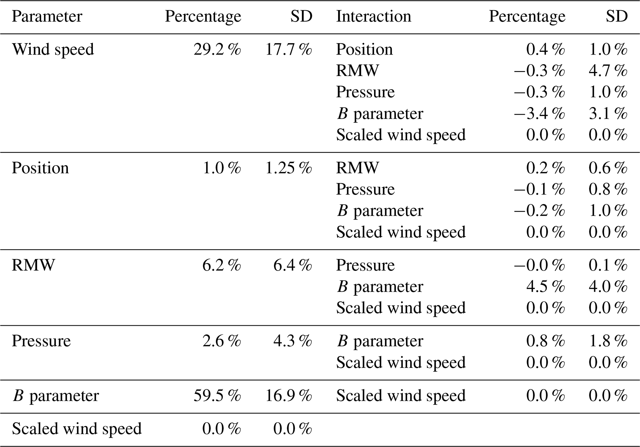
Table 12 Contribution to total uncertainty in ECUS (percentage).

5 Discussion

There have been several methods developed in the literature to estimate the extreme winds in TC-prone areas.

Studies on this subject have previously used the IBTrACS data and covered the western North Pacific Ocean, with the winds at 10 m height, as in Ott (2006) and Kong et al. (2024). This study differs from the previous by examining the entire IBTrACS data records from different agencies. The study area not only includes the western North Pacific Ocean but also the east coast of the US. We examine both the wind speeds at 10 m, in order to compare with previous studies but primarily wind speeds at 100 m, which is more relevant for modern wind turbines.

In this study, three regions were selected due to relatively high level of activities for offshore wind deployment: Taiwan, Japan, and ECUS. Given a set of data restrictions, data from IBTrACS were used as input to the Holland model. The Holland model returned a wind field for each given data point. The wind speed was scaled down to 100 m using an adjusted roughness length. To estimate the adjusted roughness length, the Holland model output was scaled to 10 m and compared against the maximum wind speed from IBTrACS. The surface roughness, which resulted in the best fit to the IBTrACS values, was selected. The standard deviation of the fit was used in the Monte Carlo simulations. As the surface roughness was selected based on comparison against 10 m data, and this study primarily focuses on wind speeds at 100 m, there is potential for further uncertainty to arise, which has not been taken into account. Following the scaling of the wind speed to 100 m, at each grid point, the annual maxima was calculated. Lastly, using the Gumbel distribution, U₅₀ was calculated as the final result.

Monte Carlo simulations were used for uncertainty analysis, where the parameters, including wind speed, position, RMW, pressure, B parameter, and scaled wind speed, were randomly varied 100 times in their 95 % confidence interval range. How well the method performed in each of the regions and the associated errors can be attributed to regional differences in TC characteristics.

The method seemed to work well for the Taiwan region in comparison to other studies. The maximum wind speed of U₅₀ at 10 m from this study was 0.7 m s⁻¹ larger than that of Ott (2006), 2.3 m s⁻¹, larger than Kong et al. (2024) and 0.3 m s⁻¹ smaller than Larsén and Ott (2022). It also presented a similar spatial distribution of winds. First, the maximum winds occur to the north-east of the Philippians. Second, the high wind speeds also extend north, while gradually weakening towards the south of Japan. Finally, there are weaker wind speeds to the west of the Philippians compared to the east of the Philippians. The three studies previously mentioned included the Japan region, also showing the peak wind speeds occurring to the south of Japan, gradually weakening as the latitude increases. The ECUS region differed from the previous two by deviating from expectations.

Here, we discuss the differences between the regions, primarily why ECUS looks to be less reliable than the other regions.

First, the focus will be on the prominent appearance of specific tracks in the ECUS region in comparison to the much weaker appearance in Japan and Taiwan. By evaluating the data availability of these regions, it becomes apparent that, per year on average, the ECUS region has the least number of data points, which can be calculated from Table 2. The smaller data count is then coupled with the wider spatial spread of data points, as shown in Fig. 6c. Following this, the ECUS neighbouring grid points can exhibit larger variations in annual maximum wind speeds compared to Japan and Taiwan. In Taiwan and Japan, the spatial gradients are generally smoother. The Gumbel distribution is fitted directly to the annual maxima at each grid point, meaning that the larger differences in annual maxima for neighbouring grid points will produce different U₅₀ estimations, causing the fragmented appearance.

Second, in ECUS, it was also expected to see the highest wind speeds consistently appear at lower latitudes due to the correlation of lower latitudes and smaller RMW (Kimball and Mulekar, 2004; Vickery and Wadhera, 2008; Pérez-Alarcón et al., 2021), which indicates stronger winds (Kimball and Mulekar, 2004; Chavas and Knaff, 2022). While this feature is not apparent, it can be explained through examination of the Holland model.

The Holland model is known to underestimate wind speeds at distances two to three times the RMW (Willoughby and Rahn, 2004) as it rapidly decreases the wind speed at these distances. The limitation becomes more pronounced when the RMW is small: the area at two to three times the RMW is still relatively close to the TC's centre, where wind speeds remain high. Therefore, the Holland model's tendency to underestimate winds reduces the accuracy of capturing the extreme wind field from small-RMW TCs. This problem further exacerbates the first issue, which is why at the lower latitudes we see smaller areas of high wind speeds.

In contrast, TCs which track farther north in the ECUS region often have larger RMW (Kimball and Mulekar, 2004) and typically have lower maximum wind speeds (Kimball and Mulekar, 2004; Chavas and Knaff, 2022). While the Holland model may still underestimate the wind speeds at two to three times the RMW, this corresponds to a distance much farther from the TC's core, where the wind speeds have already weakened. Due to this, the underestimation primarily affects less critical regions of the wind field for this study, while the important core winds are captured reasonably well.

We do not see the spatial fragmentation to the same extent occurring in the Taiwan and Japan regions, supporting the theory that the key of the issue is the smaller dataset in the ECUS region. While the underestimation of winds outside two to three times the RMW will still be present, the number of data points in Taiwan and Japan is higher, and it is consolidated into a smaller region in comparison to ECUS. The annual maxima displays reduced spatial variability between neighbouring points, which is reflected in the Gumbel distribution and the U₅₀ estimation. Therefore, it is the combination of a smaller dataset in ECUS than Taiwan and Japan, and a consistent area where small-RMW TCs occur that makes this method less reliable for the ECUS region.

This rationalisation is supported by the uncertainty analysis. As shown in Fig. 9, the RMW in the southern half of the ECUS region plays an important role in the uncertainty, whereas its influence in the Taiwan and Japan regions is much smaller (Figs. 7 and 8), even though the same methodology is applied. The larger uncertainty in the Taiwan and Japan regions comes from the B parameters. These differences reflect how regional TC characteristics influence outcomes in each of the regions.

Given that many parameters are involved in this method, the Monte Carlo simulations were effective in addressing the associated uncertainty. However, the diversity of uncertainties in the IBTrACS data makes this a challenging analysis. While the uncertainty analysis undertaken in this study may not capture all possible uncertainties, the results could provide an indication of the potential range of uncertainty, along with which parameters affect uncertainty the most. An uncertainty that has not been quantified is the results of the sampling resolution of IBTrACS. When a TC is positioned between two consecutive track points, there is no information available and therefore there are spatial gaps in the track. This could lead to underrepresentation of peak winds, particularly where storms move quickly or data are sparse. As a result, this is more likely to affect the results in the ECUS region than the Taiwan or Japan regions. Interpolating the track to a finer temporal resolution could be attempted; however, it would require assumptions about the TC evolution between observations. This in turn which would risk the introduction of greater uncertainty than that of the sampling gap. A secondary uncertainty which has not been addressed is the potential impact of climate variability on the results. While all available data have been used, this may not represent the long-term TC climate if the period coincides with an active or inactive phase of natural variability. A period of enhanced TC activity could inflate the annual maxima that is fed into the Gumbel distribution, which could return a higher U₅₀. A suppressed period would do the opposite. Although the split-half analysis revealed that the Gumbel uncertainty dominates over any detectable shift in the extreme wind climate between sub-periods, climatological variability remains an unquantified source of uncertainty.

Data availability in ECUS is heavily limited by the availability of parameter RMW, which is only recorded from 2001 onward. One way to extend the availability is to estimate the RMW using a reanalysis dataset and to integrate it with IBTrACS. Another potential option is to use a synthetic dataset, such as STORM (Bloemendaal et al., 2020b), for the analysis. A third approach is to generate a synthetic tropical cyclone database following the methodology outlined in Annex J of the IEC 61400-1 standard. However, this study was intended to specifically focus on IBTrACS data. To better capture the extreme winds from small-RMW TCs, a variation of the Holland model could be used that captures the differences between the inner core and the outer regions, as is suggested by Chavas et al. (2015).

6 Conclusions

Overall, this analysis demonstrates that combining IBTrACS data with the Holland model and the Gumbel distribution can provide a viable approach for estimating U₅₀ in some TC-affected regions. This approach is most robust in regions with substantial, spatially consolidated datasets and where RMW is not consistently small, such as in Taiwan and Japan. But in regions like ECUS, in which the dataset does not fit this criteria, the method shows limitations. Monte Carlo simulations were effective in quantifying uncertainties, highlighting the influence of region-specific TC characteristics on the results. While some uncertainties could remain unaccounted for, the approach offers insight into extreme wind estimation at heights relevant for modern wind turbines.

The key findings of this study are summarised as follows:

• The method integrates IBTrACS data, the Holland model, and the Gumbel distribution to estimate extreme wind speeds U₅₀ at 10 and 100 m, complementing previous studies.

• Data for the Taiwan and Japan regions are substantial and consolidated into a specific area, allowing for smooth spatial gradients in the annual maxima when comparing neighbouring grid points, leading to more smooth U₅₀ estimation across the regions.

• ECUS shows larger variability between neighbouring grid points due to smaller, more widely spread data points which is exacerbated at the lower latitudes due to a higher occurrence of small-RMW TCs.

• The Holland model underestimates wind speeds at distances two to three times RMW, particularly affecting small-RMW TCs and contributing to spatial fragmentation in ECUS.

• Monte Carlo simulations capture the uncertainty from input parameters, although some sources of uncertainty remain unquantified.

Future work could explore the use of alternative parametric models to better capture regional variations in TC characteristics and specifically improve performance in the ECUS region. In addition, applying the existing methodology while using larger datasets may reduce uncertainty and could provide reasonable results in the ECUS region. Using the existing methodology while comparing results using different variations of datasets would enable a systematic comparison between historical TC records and synthetic databases which represent a broader range of plausible, but unobserved, events. Finally, incorporating the influence of climate variability into the uncertainty framework is an important extension, as the current U₅₀ does not account for this.

Appendix A: Surface correction parameter calibration

The geostrophic drag law (as shown in Eq. 3) and the logarithmic wind profile (as shown in Eq. 4) both require a surface parameter z₀ to scale the gradient wind speed, which is the output of the Holland model. The gradient wind speed is first scaled 10 m for comparison with IBTrACS and subsequently to 100 m for the estimation of U₅₀. While z₀ is conventionally interpreted as the roughness length, this appendix explains why a strictly physical interpretation is possibly not appropriate here and documents the reasoning behind the calibration of this parameter. This appendix also contains a brief discussion on the quality of the resulting fit.

A physically motivated approach to estimating z₀, aligning with a standard approach, is to apply the Charnock relation at each grid point and time step for each tropical cyclone, as shown by the following equation:

$$\begin{array}{}\text{(A1)}& z_{\mathrm{0}}=\mathit{\alpha }{\displaystyle \frac{u_{*}}{g}},\end{array}$$

where z₀ is the roughness length, α is the Charnock parameter, u_* is the friction velocity, and g is gravity. To take this approach, u_* is needed and can be derived from the gradient wind speed; however, z₀ is also present in this gradient wind speed formulation. To resolve the interdependence, the gradient wind speed formulation and Charnock relation were iterated over until consistent values are found, and z₀ was also bound to a minimum of 7e⁻⁵ m (value described in Ott, 2006) and a maximum of 2e⁻⁴ m (accepted open ocean value), which are more physically reasonable values.

The resulting 10 m Holland model wind speeds were compared against the IBTrACS 10 m maximum wind speeds. The comparison revealed a systematic underestimation of the Holland 10 m wind speeds, with the distribution of percentage differences centred at approximately −10 %. Using this approach, distinct u_* and z₀ can be calculated for each grid point, at each time step for each cyclone. However, a deficit of this magnitude is incompatible with the aims of this study.

This analysis relies on annual maxima to fit the Gumbel distribution; the maximum wind speed at any given time step is the quantity most likely to be selected for inclusion in the extreme value analysis, and errors in reproducing it propagate directly into the final U₅₀ estimate. A systematic underestimation in the calibration wind speed would produce correspondingly underestimated return levels, which is less than ideal.

Given the limitations of the Charnock approach, z₀ is instead treated as an empirical surface correction parameter. It is used as a scalar that maps gradient-level Holland model winds to the 10 m level, which on average aligns with IBTrACS observations. This reinterpretation is justified by examining the Holland model. The Holland model is an empirical parametric model, so the analysis already operates outside a purely physical representation of TC wind structure.

Calibration is performed by identifying the value of z₀ for each region that minimises the mean percentage difference between the scaled Holland model 10 m wind speed and the IBTrACS 10 m maximum wind speed across all available data points. The surface correction parameters identified are $\mathrm{5}\times {\mathrm{10}}^{-\mathrm{6}}$, $\mathrm{9}\times {\mathrm{10}}^{-\mathrm{6}}$, and $\mathrm{1}\times {\mathrm{10}}^{-\mathrm{5}}$ m for the Taiwan, Japan, and ECUS regions, respectively.

A key constraint on this calibration is that IBTrACS provides only the maximum wind speed at each time step; no spatial wind field is available. Calibration can therefore only be performed at the location of the maximum wind speed. Extending the calibrated z₀ spatially through additional assumptions would introduce further unquantifiable uncertainty and is not pursued here.

The value z₀ does not vary between times steps or TCs. This route was pursued because fitting the parameter to time steps or individual events would risk absorbing errors originating from both the Holland model and IBTrACS into the parameter itself and could produce unstable values. A single spatially uniform and temporally constant value is therefore adopted for each region. This ensures that variability in the U₅₀ results is driven by the statistics of the storm population rather than by the tuning of the surface parameter. The standard deviation of the residuals from the calibration fit is used as the uncertainty estimate for the scaled wind speed in the Monte Carlo analysis, as shown in Table 9.

Figure A1 presents the probability density distributions of the differences between the scaled 10 m Holland wind speed and the IBTrACS 10 m values, calculated by the following equation:

$$\begin{array}{}\text{(A2)}& \mathrm{\Delta }u=\mathrm{100}\times \left({\displaystyle \frac{u_{\mathrm{Holland}}-u_{\mathrm{IBTrACS}}}{u_{\mathrm{IBTrACS}}}}\right).\end{array}$$

In all regions, 98.8 % or more of the Holland model 10 m maximum wind speeds fall within ±10 % of the corresponding IBTrACS value. This level of agreement is best understood in relation to the observational uncertainty inherent in IBTrACS itself. As documented in the IBTrACS technical documentation (IBTrACS Science Team, 2025) and summarised in Table 5, wind speed uncertainties since the year 2000 are approximately ±7 kt in the northern Atlantic and ±10 kt in the western Pacific. For category 5 storms, these correspond to approximately ±5 % and ±7 %, respectively; for category 1 storms, these correspond to ±9 % and ±12 %, respectively, closely aligning with the error when scaling the gradient Holland model wind speeds.

A further feature of the distributions in Fig. A1 is that they are not all perfectly symmetric about zero in all regions. In the Taiwan region, the results look mostly symmetrical, with 45.3 % of values falling above 0. In the Japan region, slightly skew appears to the right; however, 46.6 % of values fall above 0. Lastly, in the ECUS region, the distribution skews to the left, and 71 % of data points are above 0. This means that the Holland-model-scaled wind speeds tend to exceed the IBTrACS reference; however, this is a favourable outcome. A marginal positive bias in the calibration wind speed propagates to slightly elevated annual maxima and, consequently, slightly elevated U₅₀ estimates. Conservatism is likely desirable in the context of offshore infrastructure assessment.

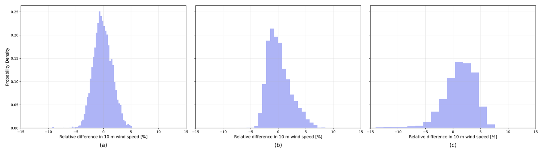
Figure A1 Comparison of maximum 10 m wind speeds from the Holland model and IBTrACS. The panels show the probability density distributions of the percentage difference Δu for (a) Taiwan, (b) Japan, and (c) ECUS.

Appendix B: Abbreviations

Abbreviation	Full name
CFSR	Climate Forecast System Reanalysis
CMA	China Meteorological Administration
ECUS	East coast of the US
ERA5	European Centre for Medium-Range Weather Forecast Reanalysis v5
IBTrACS	International Best Track Archive for Climate Stewardship
IEC	International Electrotechnical Commission
JMA	Japan Meteorological Agency
HKO	Hong Kong Observatory
MERRA 2	Modern-Era Retrospective Analysis for Research and Applications
NOAA	National Oceanic and Atmospheric Administration
RMW	Radius of maximum winds
TC	Tropical cyclone
US	United States