Concurrent aerodynamic design of the wing and the turbines of airborne wind energy systems

The aerodynamic design of the fly-gen airborne wind energy system aircraft, referred to as a windplane here, is a largely unexplored yet crucial problem for improving power production. To this end, an engineering model for the aerodynamics of the onboard turbines, the aerodynamics of the wing, and their interactional aerodynamics is developed and coupled to a steady-state windplane model and a far-wake model. This novel comprehensive model is then used to design the windplane aerodynamics for a given wingspan. Initially, a design space exploration study reveals that placing the turbines at the wing tips and rotating them inboard down increases the power production compared to other locations and rotation directions. This improvement arises because the turbines' wake swirl reduces the wing's induced drag, which increases flight speed and, consequently, the generated power. Moreover, airfoils with a high lift-to-drag ratio are found to be optimal for windplanes. As a consequence, NACA4421 airfoils are used for the design of the wing and the tip-mounted turbines. The trapezoidal wing with constant twist which maximizes power production has an aspect ratio of 5.1 and a taper ratio of 0.60. By design, the onboard turbines operate at a low tip speed ratio of 1.9 to increase the wake swirl. The results from the vortex models of the wing, the turbines, and their interaction show very good agreement with the lifting line, the vortex lattice method, and the vortex particle method implemented in the well-established code DUST. Finally, the windplane is studied with DUST at different wing angles of attack and at different turbine tip speed ratios to characterize its behavior away from the design point. The maximum in power production is observed near to the design point, well separated from the stall regions of both the wing and the turbines.

1 Introduction

Airborne wind energy systems (AWESs) harvest wind power by means of a fully autonomous aircraft connected to the ground by a tether. AWESs can be classified as crosswind, tether aligned, or rotational (Vermillion et al., 2021). Most industrial and research activities focus on crosswind AWESs, whose working principles were first described by Loyd (1980). Crosswind AWESs move in a fast motion roughly perpendicular to the wind direction and generate power either with onboard small wind turbines (fly-gen AWESs), as studied in this paper, or by pulling the tether and unwinding a generator on the ground (pumping AWESs). For more details, Fagiano et al. (2022) give an overview of the state of the art of these systems.

Fly-gen AWESs fly figure-of-eight or circular trajectories and generate power with the onboard turbines. The electrical power is transmitted to the ground via the tether, which has both a structural and an electrical component. The aircraft of fly-gen AWESs is termed to be a windplane in this paper. It is a rather unique system, whose design is far from being fully understood. This is due to the need to operate in very different phases (take-off and landing, power production, transitions) and at a broad range of wind speeds and to maximize the converted power while meeting structural and controllability requirements. Currently, fly-gen systems are actively developed by companies such as Kitekraft GmbH (2025) and WindLift (2025) and were developed by Makani Technologies LLC (2025), which ceased operations in 2020.

KiteKraft's design is based on a box wing, with turbines that are distributed along the span of both wings. The AWES flies figure-of-eight trajectories and operates the windplane at very high lift coefficients (C_L≈4.5), achieved through multi-element airfoils (Bauer et al., 2018). The onboard turbines are designed for the power generation and to sustain the AWES during hover but not in conjunction with the wing design (Frirdich, 2019). The WindLift design is not disclosed, and only a limited amount of information is publicly available. Their design is characterized by a single wing with four turbines mounted on pylons. On the other hand, the Makani's development is well documented in publicly available sources. After the shut-down, Makani engineers released two reports summarizing the design, analyses, and testing methodologies (Echeverri et al., 2020a, and Echeverri et al., 2020b). Makani's last prototype, the M600, had a wingspan of 26 m, an aspect ratio of 20, and eight turbines mounted on pylons along the wing. Before the shut-down, Makani engineers re-designed the AWES to overcome major shortcomings, resulting in the MX2 design. The MX2 was designed to feature a wingspan of 26 m, an aspect ratio of 12.5, and eight turbines. The wings' and turbines' designs were carried out separately. The turbines are designed to generate power and to provide the thrust to sustain the AWES during hover. Their wing is designed to maximize the power-harvesting factor¹, as explained by Tucker (2020) and in an earlier paper by Vander Lind (2013). The power-harvesting factor is defined by Diehl (2013) as the ratio between the generated power and the kinetic energy flux (or wind power density) passing through the wing planform area. This definition is purely a normalization choice since no actual flow passes through the planform area, which is, however, used as a reference area for normalization. Wings designed to maximize the power-harvesting factor have a high aspect ratio (Echeverri et al., 2020a; Bauer et al., 2018; Fasel et al., 2017; Trevisi et al., 2021, among others) and use unconventional airfoils, which are designed to maximize the metric $C_{\mathrm{l}}^{\mathrm{3}}/C_{\mathrm{d}}^{\mathrm{2}}$ (Bauer et al., 2018; De Fezza and Barber, 2022; Porta Ko et al., 2023; Rangriz and Kheiri, 2025, among others).

Recently, Trevisi (2024) introduced a new design methodology for windplanes, performing the aerodynamic design per a given wingspan. This is achieved by maximizing a new power coefficient², defined as the ratio between the generated power and the kinetic energy flux (or wind power density) passing through a disk with a radius equal to the wingspan (Trevisi et al., 2023a). This reference area does not correspond to an actual flow cross-section but is just used as a reference area to normalize the generated power. Wings designed to maximize this power coefficient have low aspect ratios (approximately between 4 and 7) and use conventional efficient airfoils (i.e., airfoils with high $C_{\mathrm{l}}/C_{\mathrm{d}}$). This new methodology is improved in this paper to concurrently design the main wing and the onboard turbines. Three turbine positions are considered: in front of the wing's leading edge at half the semi-wing span, at the wing tips, and above or below the wing. If they are placed above or below, they need pylons, which have an associated aerodynamic drag and decrease the system performances. If they are placed in front of the wing, they reduce the apparent wind speed experienced by the involved wing aerodynamic sections, which reduces lift force. Conversely, airplanes with propellers in front of the wing achieve an increase in aerodynamic lift. Another relevant aerodynamic effect is the swirl in the turbine wake. Airplane designers have long exploited this effect by placing the onboard propellers at the wing tips (Snyder and Zumwalt, 1969; Patterson and Bartlett, 1985), allowing the downstream aerodynamic sections to experience a beneficial change in inflow angle, leading to a decrease in induced drag. Miranda and Brennan (1986) started the theoretical and numerical investigation of the decrease in induced drag due to tip propellers and tip turbines. They developed a vortex model similar to the one presented in this paper to assess the benefit of placing the rotors at the wing tips. Recently, Sinnige et al. (2019b) performed wind tunnel tests comparing tip propeller configurations to conventional layouts and studied their performance under energy-harvesting conditions (Sinnige et al., 2019a). Taking inspiration from this aeronautical experience, here, we design the windplane onboard turbines with engineering models. We design the rotors for the generation phase only and do not consider whether they generate enough thrust in the hover state. This is done to focus on the ideal aerodynamic design of the windplane to fulfill its main functionality, i.e., power generation. The design can be modified later to cope with the take-off and landing phases, which are less demanding in terms of power ratings (Fagiano and Schnez, 2017). We validate the proposed framework with the lifting line, the vortex lattice method, and the vortex particle method implemented in DUST (Tugnoli et al., 2021). This code is open-source and has been validated for wing propeller studies (Niro et al., 2024). Finally, we use DUST to characterize the wing and rotor design away from the design point. The vortex particle method has recently been used by Mehr et al. (2024) to analyze the Makani prototype (characterized by rotors mounted on pylons) and to investigate the effects of rotor rotation direction and vertical and streamwise rotor position on the overall aerodynamic performance without however moving the rotors in front of the wing and along the wing span.

This paper is organized as follows: in Sect. 2, the aerodynamic modeling framework is introduced; in Sect. 3, the aerodynamic optimization problem formulation is introduced, and a design space exploration study on the turbine positions and on the optimal airfoil characteristics is carried out; in Sect. 4, the vortex particle code DUST, used for validation and analysis, is introduced; in Sect. 5, the optimal design problem is solved, the solution is compared with DUST, and the design is studied away from the design point; in Sect. 6, the main conclusions are discussed, and future work is suggested. A list of symbols is given at the end of the paper.

2 Windplane aerodynamics model

We start by formulating the modeling framework for the optimal design problem of the wing and the rotors. The model is meant to be as simple as possible while still capturing the relevant physical phenomena.

2.1 Windplane steady-state model

We assume a steady-state equilibrium, neglecting gravity and assuming a circular fully crosswind trajectory with steady uniform wind. Indeed, Trevisi (2024) shows that the aerodynamic problem is not influenced by the dynamic problem. Referring to Fig. 1, the force balance is written in the cylindrical coordinate system $({\mathit{e}}_{\mathit{\theta }},{\mathit{e}}_{\mathrm{r}},{\mathit{e}}_z)$, where e_θ points tangentially, e_r points radially, and e_z points axially.

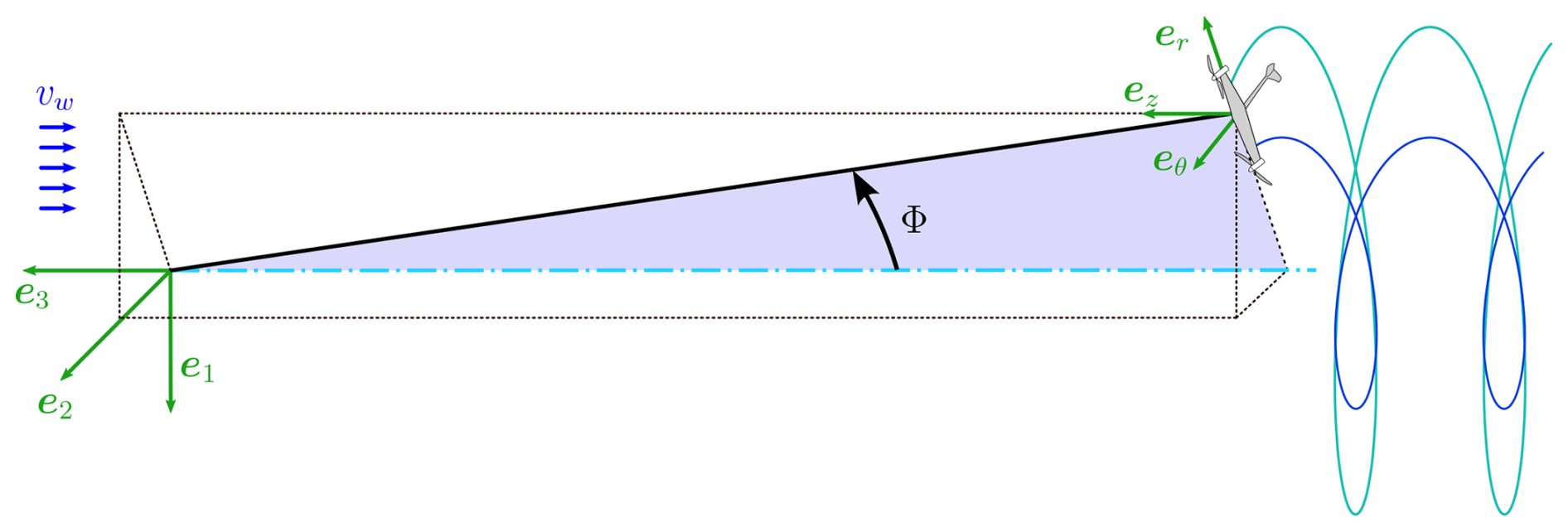
Figure 1 Ground coordinate system $({\mathit{e}}_{\mathrm{1}},{\mathit{e}}_{\mathrm{2}},{\mathit{e}}_{\mathrm{3}})$ and cylindrical coordinate system $({\mathit{e}}_{\mathit{\theta }},{\mathit{e}}_{\mathrm{r}},{\mathit{e}}_z)$. v_w is the incoming wind speed, and Φ is the opening angle of the circular trajectory, centered on the light-blue dash-dotted line. The light- and dark-blue helices represent the right- and left-trailed vortices.

The aerodynamic forces and the main wake components are shown in Fig. 2. Considering the velocity triangle and the inflow angle in the near wake γ_n, the force balances in the three axes are

$$\begin{array}{}\text{(1)}& \left\{\begin{array}{l}L\sin {\mathit{\gamma }}_{\mathrm{n}}-(D_{\mathrm{p}}+D_{\mathrm{i}}+T_{\mathrm{t}})\cos {\mathit{\gamma }}_{\mathrm{n}}=\mathrm{0}\\ m\frac{u^{\mathrm{2}}}{R_{\mathrm{0}}}=T_z\tan \left(\mathrm{\Phi }\right)\\ T_z=L\cos {\mathit{\gamma }}_{\mathrm{n}}+(D_{\mathrm{p}}+D_{\mathrm{i}}+T_{\mathrm{t}})\sin {\mathit{\gamma }}_{\mathrm{n}}\end{array}\right.,\end{array}$$

where L is the aerodynamic lift, D_p is the parasite drag, D_i is the induced drag, T_t is the turbine thrust, m is the system mass (equal to the aircraft mass plus one-third of the tether mass, as derived from Trevisi et al., 2020), u is the tangential velocity, R₀ is the trajectory radius, T_z is the axial component of the tether force, and Φ is the opening angle of the circular trajectory.

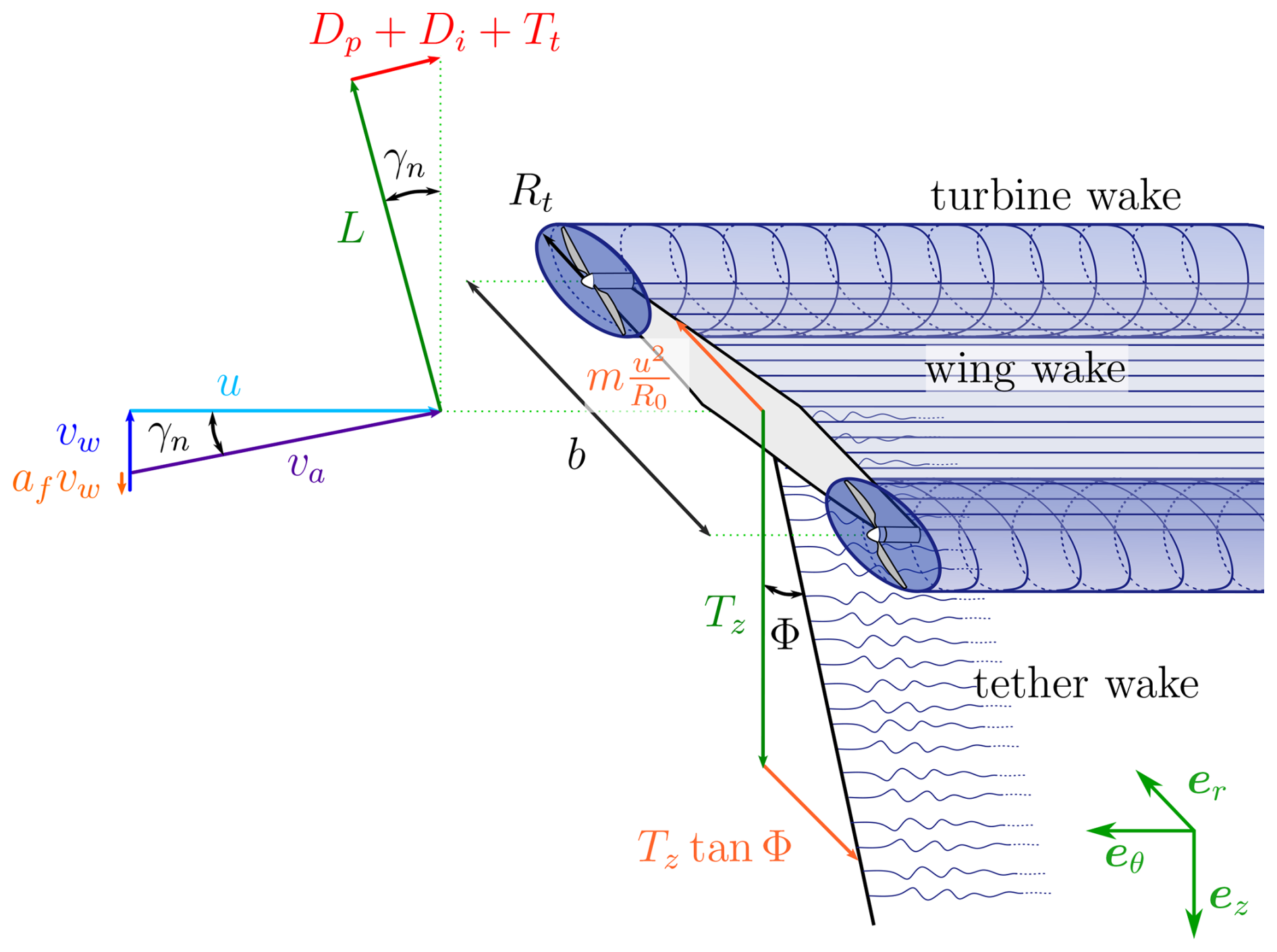
Figure 2 Velocity triangle, forces acting on the windplane in crosswind steady-state and main wake components.

The aerodynamic lift L, defined to be perpendicular to the apparent velocity v_a, is

$$\begin{array}{}\text{(2)}& L={\displaystyle \frac{\mathrm{1}}{\mathrm{2}}}\mathit{\rho }A{C}_{\mathrm{L}}{v}_{\mathrm{a}}^{\mathrm{2}},\end{array}$$

where ρ is the air density, C_L is the wing lift coefficient, and the wing area A is

$$\begin{array}{}\text{(3)}& A={\displaystyle \frac{b^{\mathrm{2}}}{\mathrm{AR}}},\end{array}$$

where b is the wing span, and AR is the wing aspect ratio.

The aerodynamic parasite drag is

$$\begin{array}{}\text{(4)}& D_{\mathrm{p}}={\displaystyle \frac{\mathrm{1}}{\mathrm{2}}}\mathit{\rho }A{C}_{\mathrm{D},\mathrm{p}}{v}_{\mathrm{a}}^{\mathrm{2}},\end{array}$$

where C_D,p is the parasite drag coefficient, defined as

$$\begin{array}{}\text{(5)}& C_{\mathrm{D},\mathrm{p}}=C_{\mathrm{D},\mathrm{a}}+C_{\mathrm{D},\mathrm{te}}.\end{array}$$

C_D,a is the three-dimensional coefficient due to the airfoils, and C_D,te is the equivalent tether drag (Trevisi et al., 2020):

$$\begin{array}{}\text{(6)}& C_{\mathrm{D},\mathrm{te}}=C_{\mathrm{d},\mathrm{te}}{\displaystyle \frac{L_{\mathrm{te}}{D}_{\mathrm{te}}}{\mathrm{4}A}},\end{array}$$

where C_d,te is the tether section drag coefficient, L_te is the tether length, and D_te is the tether diameter.

The induced drag is

$$\begin{array}{}\text{(7)}& D_{\mathrm{i}}={\displaystyle \frac{\mathrm{1}}{\mathrm{2}}}\mathit{\rho }A{C}_{\mathrm{D},\mathrm{i}}{v}_{\mathrm{a}}^{\mathrm{2}},\end{array}$$

where C_D,i is the induced drag coefficient of the near wake. Indeed, Trevisi et al. (2023b) show that the induced velocities due to the near wake (first half rotation of the helicoidal wake shown in Fig. 1) can be taken into account with an induced drag coefficient computed assuming the trailed vortex filaments as straight, as done in this work. More details about this modeling approach are given in Sect. 2.4.

The thrust force produced by the onboard wind turbines is

$$\begin{array}{}\text{(8)}& T_{\mathrm{t}}={\displaystyle \frac{\mathrm{1}}{\mathrm{2}}}\mathit{\rho }{A}_{\mathrm{t}}{C}_{\mathrm{T},\mathrm{t}}{v}_{\mathrm{a}}^{\mathrm{2}},\end{array}$$

where C_T,t is the thrust coefficient of the onboard wind turbines, and A_t is the total rotor area. We define the onboard wind turbine radius as a function of the wing semi-span as

$$\begin{array}{}\text{(9)}& R_{\mathrm{t}}={\mathit{\xi }}_{\mathrm{t}}{\displaystyle \frac{b}{\mathrm{2}}},\end{array}$$

where the total rotor area A_t, assuming two turbines n_t=2, is

$$\begin{array}{}\text{(10)}& A_{\mathrm{t}}=n_t\mathit{\pi }{R}_{\mathrm{t}}^{\mathrm{2}}={\displaystyle \frac{\mathit{\pi }{\mathit{\xi }}_{\mathrm{t}}^{\mathrm{2}}}{\mathrm{2}}}{b}^{\mathrm{2}}.\end{array}$$

In this work, we assume two turbines to simplify the problem as much as possible. However, the modeling framework is general, and different configurations might be investigated.

The employed model to estimate the thrust coefficient C_T,t of the onboard turbines is described in Sect. 2.2, while the models for the aerodynamic coefficients C_D,a and C_D,i are detailed in Sect. 2.3.

The force balance along the tangential direction (first component in Eq. 1) can be written as

$$\begin{array}{}\text{(11)}& \tan {\mathit{\gamma }}_{\mathrm{n}}={\displaystyle \frac{D_{\mathrm{p}}+D_{\mathrm{i}}+T_{\mathrm{t}}}{L}}={\displaystyle \frac{\mathrm{1}}{E}},\end{array}$$

where E is the windplane aerodynamic efficiency, including the thrust of the turbines.

The inflow angle in the near wake, γ_n, can be found by considering the tangential velocity to the plane's path u and by subtracting the induced velocity due to the far wake a_fv_w from the free wind velocity v_w (Trevisi et al., 2023b):

$$\begin{array}{}\text{(12)}& \tan {\mathit{\gamma }}_{\mathrm{n}}={\displaystyle \frac{v_{\mathrm{w}}(\mathrm{1}-a_{\mathrm{f}})}{u}}={\displaystyle \frac{(\mathrm{1}-a_{\mathrm{f}})}{\mathit{\lambda }}},\end{array}$$

where $\mathit{\lambda }=\frac{u}{v_{\mathrm{w}}}$ is the wing speed ratio.

The wing speed ratio λ can be found by equating Eqs. (11) and (12) and using the definition of the aerodynamic forces:

$$\begin{array}{}\text{(13)}& \begin{array}{rl}\mathit{\lambda }=E(\mathrm{1}-a_{\mathrm{f}})& ={\displaystyle \frac{\frac{\mathrm{1}}{\mathrm{2}}\mathit{\rho }A{C}_{\mathrm{L}}{v}_{\mathrm{a}}^{\mathrm{2}}(\mathrm{1}-a_{\mathrm{f}})}{\frac{\mathrm{1}}{\mathrm{2}}\mathit{\rho }A(C_{D,p}+C_{\mathrm{D},\mathrm{i}}+\frac{A_{\mathrm{t}}}{A}{C}_{\mathrm{T},\mathrm{t}})v_{\mathrm{a}}^{\mathrm{2}}}}\\ & ={\displaystyle \frac{C_{\mathrm{L}}(\mathrm{1}-a_{\mathrm{f}})}{C_{D,p}+C_{\mathrm{D},\mathrm{i}}+\frac{\mathit{\pi }}{\mathrm{2}}\mathrm{AR}{\mathit{\xi }}_{\mathrm{t}}^{\mathrm{2}}{C}_{\mathrm{T},\mathrm{t}}}}.\end{array}\end{array}$$

The power equation can be written with respect to the onboard turbines as

$$\begin{array}{}\text{(14)}& \begin{array}{rl}P& ={\displaystyle \frac{\mathrm{1}}{\mathrm{2}}}\mathit{\rho }{A}_{\mathrm{t}}{C}_{\mathrm{P},\mathrm{t}}{v}_{\mathrm{a}}^{\mathrm{3}}\approx {\displaystyle \frac{\mathrm{1}}{\mathrm{2}}}\mathit{\rho }{A}_{\mathrm{t}}{C}_{\mathrm{P},\mathrm{t}}{\mathit{\lambda }}^{\mathrm{3}}{v}_{\mathrm{w}}^{\mathrm{3}}\\ & ={\displaystyle \frac{\mathrm{1}}{\mathrm{2}}}\mathit{\rho }{A}_{\mathrm{t}}{C}_{\mathrm{P},\mathrm{t}}{E}^{\mathrm{3}}(\mathrm{1}-a_{\mathrm{f}}{)}^{\mathrm{3}}{v}_{\mathrm{w}}^{\mathrm{3}},\end{array}\end{array}$$

where C_P,t is the power coefficient of the onboard wind turbines, and large values of λ are assumed (λ²≫1). In practice, the wing speed ratio ranges from λ≈5 to λ≈10, thus justifying this assumption.

The windplane power coefficient, using as a reference area the disk with the radius of the wingspan (Trevisi et al., 2023a), is

$$\begin{array}{}\text{(15)}& C_P={\displaystyle \frac{P}{\frac{\mathrm{1}}{\mathrm{2}}\mathit{\rho }\mathit{\pi }{b}^{\mathrm{2}}{v}_{\mathrm{w}}^{\mathrm{3}}}}=C_{\mathrm{P},\mathrm{t}}{\displaystyle \frac{{\mathit{\xi }}_{\mathrm{t}}^{\mathrm{2}}}{\mathrm{2}}}{\mathit{\lambda }}^{\mathrm{3}}=C_{\mathrm{P},\mathrm{t}}{\displaystyle \frac{{\mathit{\xi }}_{\mathrm{t}}^{\mathrm{2}}}{\mathrm{2}}}{E}^{\mathrm{3}}(\mathrm{1}-a_{\mathrm{f}}{)}^{\mathrm{3}}.\end{array}$$

The windplane thrust coefficient, similar to the conventional turbines' thrust coefficient, is defined to inform us about the aerodynamic force which does work to the wind (i.e., the component of the aerodynamic force which is parallel to the wind direction and thus slows it down) as follows:

$$\begin{array}{}\text{(16)}& C_{\mathrm{T}}={\displaystyle \frac{T_z}{\frac{\mathrm{1}}{\mathrm{2}}\mathit{\rho }\mathit{\pi }{b}^{\mathrm{2}}{v}_{\mathrm{w}}^{\mathrm{2}}}}\approx {\displaystyle \frac{C_{\mathrm{L}}}{\mathit{\pi }\mathrm{AR}}}{\mathit{\lambda }}^{\mathrm{2}}={\displaystyle \frac{C_{\mathrm{L}}}{\mathit{\pi }\mathrm{AR}}}{E}^{\mathrm{2}}(\mathrm{1}-a_{\mathrm{f}}{)}^{\mathrm{2}},\end{array}$$

where small inflow angles in the near wake, i.e., γ_n≪1, are assumed, such that the axial component of the tether force can be approximated with the lift force T_z≈L (third component in Eq. 1). Writing the turning radius as R₀=L_tesin Φ, the radial equilibrium (second component in Eq. 1) can be formulated to find the opening angle Φ such that the wingspan is fully crosswind (i.e., the lift is not used for turning):

$$\begin{array}{}\text{(17)}& \sin \mathrm{\Phi }\tan \mathrm{\Phi }={\displaystyle \frac{m}{\frac{\mathrm{1}}{\mathrm{2}}\mathit{\rho }A{C}_{\mathrm{L}}{L}_{\mathrm{te}}}}.\end{array}$$

2.2 Onboard-turbine model

In order to evaluate the onboard turbines' performance and the effect of their wakes on the wing, we use the vortex cylinder model introduced by Branlard and Gaunaa (2016), which accounts for the radially varying circulation by superposing the vortex cylinder models developed by Branlard and Gaunaa (2015). The model is an actuator disk model like the momentum-based framework that blade element momentum (BEM) models are based on. The added value provided by the vortex cylinder model is that it includes the effect of the pressure drop due to wake rotation that is neglected in the momentum-based models. The importance of this effect increases as the tip speed ratio is decreased, which is when the wake rotation increases.

Let us define the parameter k as $k\left(r_t\right)\equiv \frac{{\mathrm{\Omega }}_{\mathrm{t}}{\mathrm{\Gamma }}_t\left(r_t\right)}{\mathit{\pi }{u}^{\mathrm{2}}}$, where Γ_t(r_t) is the bound circulation of the annulus, Ω_t is the rotor angular velocity, u is the inflow velocity into the rotor, and $r_t\in [\mathrm{0},R_{\mathrm{t}}]$ is the radial coordinate. Then, the rotor quantities can be evaluated for a given radial distribution of the parameter k(r_t) and a given tip speed ratio ${\mathit{\lambda }}_{\mathrm{t}}=\frac{{\mathrm{\Omega }}_{\mathrm{t}}{R}_{\mathrm{t}}}{u}$. The tangential induction at the turbine radius r_q can be evaluated for a given value of k_q(r_q) as

$$\begin{array}{}\text{(18)}& a_{t,q}^{\prime }={\displaystyle \frac{k_q}{\mathrm{4}{\mathit{\lambda }}_{r_q,t}^{\mathrm{2}}}},\end{array}$$

where the local speed ratio is ${\mathit{\lambda }}_{r_q,t}={\mathit{\lambda }}_{\mathrm{t}}\frac{r_q}{R_{\mathrm{t}}}$. The dimensional tangential velocity (swirl) at the rotor disk can then be evaluated as

$$\begin{array}{}\text{(19)}& w_{t,q}=a_{t,q}^{\prime }{\mathit{\lambda }}_{r_q,t}u.\end{array}$$

The local thrust coefficient is defined as

$$\begin{array}{}\text{(20)}& C_{t,q}\equiv k_q\left(\mathrm{1}+{\displaystyle \frac{k_q}{\mathrm{4}{\mathit{\lambda }}_{r_q,t}^{\mathrm{2}}}}\right),\end{array}$$

such that the rotor thrust coefficient is

$$\begin{array}{}\text{(21)}& C_{\mathrm{T},\mathrm{t}}={\displaystyle \frac{\mathrm{1}}{\mathit{\pi }{R}_{\mathrm{t}}^{\mathrm{2}}}}\sum _q{C}_{t,q}\mathit{\pi }\left(r_{q+\mathrm{1}}^{\mathrm{2}}-r_q^{\mathrm{2}}\right).\end{array}$$

The effect of the rotation of the wake is a decrease in the pressure toward the rotational axis. The part of the local thrust coefficient corresponding to this is the rotational thrust coefficient, which is

$$\begin{array}{}\text{(22)}& C_{t,\mathrm{rot},q}\equiv \sum _{j>q}{\left({\displaystyle \frac{k_j}{\mathrm{2}}}\right)}^{\mathrm{2}}\left[{\displaystyle \frac{\mathrm{1}}{{\mathit{\lambda }}_{r_{j-\mathrm{1}},t}^{\mathrm{2}}}}-{\displaystyle \frac{\mathrm{1}}{{\mathit{\lambda }}_{r_j,t}^{\mathrm{2}}}}\right].\end{array}$$

The induction at each radial station is

$$\begin{array}{}\text{(23)}& a_{t,q}={\displaystyle \frac{\mathrm{1}}{\mathrm{2}}}\left(\mathrm{1}-\sqrt{\mathrm{1}-C_{t,q}+C_{t,\mathrm{rot},q}}\right),\end{array}$$

such that the reduction in axial velocity at the rotor disk is

$$\begin{array}{}\text{(24)}& u_{t,q}=a_{t,q}u.\end{array}$$

The local power coefficient is

$$\begin{array}{}\text{(25)}& C_{p,q}=k_q\left(\mathrm{1}-a_q\right),\end{array}$$

and the rotor power coefficient is

$$\begin{array}{}\text{(26)}& C_{\mathrm{P},\mathrm{t}}={\displaystyle \frac{\mathrm{1}}{\mathit{\pi }{R}_{\mathrm{t}}^{\mathrm{2}}}}\sum _q{C}_{p,q}\mathit{\pi }\left(r_{q+\mathrm{1}}^{\mathrm{2}}-r_q^{\mathrm{2}}\right).\end{array}$$

This model enables the estimation of the turbine thrust coefficient C_T,t (Eq. 21) and the power coefficient C_P,t (Eq. 26) for a given distribution of the parameter k(r_t) and tip speed ratio λ_t. Moreover, it provides the velocities induced in the turbine wake³, which are twice the velocities in the rotor disk. Veldhuis (2004) highlights that a swirl recovery factor of $\mathrm{1}/\mathrm{2}$ should be included to properly model the rotor-wing interaction, when the velocities in the rotor wake are considered to be inputs into the wing. The reduction in the slipstream induction and swirl can be attributed to the wing-induced upwash. The correct induced velocities to be used as inputs for the wing are then the induced velocities in the rotor disk. This is explained by Miranda and Brennan (1986) as a generalization of Munk stagger theorem (Prandtl, 1924), which is used to compute the induced drag of multiple wings (e.g., main wing and horizontal stabilizer). This theorem states that the total induced drag of systems of multiple wings with a fixed Trefftz-projected bound circulation is independent of the streamwise location of each of the wings. This shows that the total induced drag of a multiple-wing system can be calculated by moving the wings to the same streamwise position. Similarly, the correct induced drag of the rotor–wing system in the present case is calculated by moving the rotors to the same streamwise position as that of the wing. For this reason, the induced velocities w_t and u_t (Eqs. 19 and 24), which are the values at the rotor disk (equal to half the values in the turbine far wake), are used as inputs for the wing.

These considerations also point out that placing the turbines after the wing would not change the overall induced drag as long as they are placed in the same stream-wise location. Thus, in this paper, we only study the case in which the rotors are placed in front of the wing.

2.3 Wing model

Here, we introduce the wing model, based on the lifting-line theory of Weissinger (1947). An infinitesimal segment of vortex filament dl, located at l and with vortex strength Γ, induces a velocity dV at an arbitrary point P. Defining the distance from dl to P as r, the induced velocity dV can be evaluated with the Biot–Savat law:

$$\begin{array}{}\text{(27)}& \mathrm{d}\mathit{V}={\displaystyle \frac{\mathrm{\Gamma }}{\mathrm{4}\mathit{\pi }}}{\displaystyle \frac{\mathrm{d}\mathit{l}\times \mathit{r}}{|\mathit{r}{|}^{\mathrm{3}}}}.\end{array}$$

Referring to Fig. 3, we model the wing as a straight lifting line pointing along the y direction, discretized in N_p elements, with N_p being an even number. The chord direction of the airfoil at the wing center is taken to be equal to the x direction. Each element p is characterized by a bound vortex of strength Γ_p located along the direction of the quarter-chord line. According to the Helmholtz's vortex theorem, a vortex must extend to the boundaries of the fluid so that each element trails two vortexes of strength equal to Γ_p from its extremes. The number of trailed vortices is then N_p+1, with intensity γ_p = ${\mathrm{\Gamma }}_p-{\mathrm{\Gamma }}_{p-\mathrm{1}}$. According to Pistolesi's theorem, following the implementation by Damiani et al. (2019), we evaluate the induced velocities at the chord-wise position of the three-quarter chord of each element. The distance r of the evaluation point ${\mathit{P}}_j=[-\frac{c_j}{\mathrm{2}};y_j;\mathrm{0}]$ with respect to the reference system placed on the quarter-chord line from a generic point located at $\mathit{l}=[x;y;\mathrm{0}]$ is

$$\begin{array}{}\text{(28)}& \mathit{r}=\left[\begin{array}{c}-\frac{c_j}{\mathrm{2}}-x\\ y_j-y\\ \mathrm{0}\end{array}\right]=r_j\left[\begin{array}{c}-\sin {\mathit{\theta }}_j\\ \cos {\mathit{\theta }}_j\\ \mathrm{0}\end{array}\right],\end{array}$$

with the angle θ_j being

$$\begin{array}{}\text{(29)}& \tan {\mathit{\theta }}_j={\displaystyle \frac{\frac{c_j}{\mathrm{2}}+x}{y_j-y}}.\end{array}$$

The velocity induced by an infinitesimal portion of the bound vortex located at $\mathit{l}=[\mathrm{0};y;\mathrm{0}]$ at the evaluation point P_j can be evaluated with Eq. (27), where $d\mathit{l}=[\mathrm{0};dy;\mathrm{0}]$ and r are given in Eq. (28):

$$\begin{array}{}\text{(30)}& d{w}_j{|}_{\mathrm{bound}}={\displaystyle \frac{\mathrm{\Gamma }}{\mathrm{4}\mathit{\pi }}}{\displaystyle \frac{\sin {\mathit{\theta }}_j}{{r_j}^{\mathrm{2}}}}\mathrm{d}y={\displaystyle \frac{\mathrm{\Gamma }}{\mathrm{4}\mathit{\pi }}}{\displaystyle \frac{\sin {\mathit{\theta }}_j}{c_j/\mathrm{2}}}\mathrm{d}{\mathit{\theta }}_j,\end{array}$$

with $\mathrm{d}y=\frac{\mathrm{1}}{c_j/\mathrm{2}}\frac{(y_j-y{)}^{\mathrm{2}}}{{\cos }^{\mathrm{2}}{\mathit{\theta }}_j}\mathrm{d}{\mathit{\theta }}_j$ being obtained by differentiating Eq. (29) with x=0.

The velocity induced by the finite bound vortex p is then

$$\begin{array}{}\text{(31)}& \begin{array}{rl}\mathrm{\Delta }{w}_{p,j}{|}_{\mathrm{bound}}=& {\displaystyle \frac{{\mathrm{\Gamma }}_p}{\mathrm{4}\mathit{\pi }}}{\displaystyle \frac{\mathrm{1}}{c_j/\mathrm{2}}}\underset{{\mathit{\theta }}_{p,j}}{\overset{{\mathit{\theta }}_{p+\mathrm{1},j}}{\int }}\sin {\mathit{\theta }}_{j}d{\mathit{\theta }}_j\\ =& -{\displaystyle \frac{{\mathrm{\Gamma }}_p}{\mathrm{4}\mathit{\pi }}}{\displaystyle \frac{\cos {\mathit{\theta }}_{p+\mathrm{1},j}-\cos {\mathit{\theta }}_{p,j}}{c_j/\mathrm{2}}}.\end{array}\end{array}$$

The velocity induced by the trailed vortex p at the evaluation point P_j is evaluated by integrating Eq. (27), where $\mathrm{d}\mathit{l}=[\mathrm{d}x;\mathrm{0};\mathrm{0}]$ and r are given in Eq. (28):

$$\begin{array}{}\text{(32)}& \begin{array}{rl}\mathrm{\Delta }{w}_{p,j}{|}_{\mathrm{trailed}}& ={\displaystyle \frac{{\mathit{\gamma }}_p}{\mathrm{4}\mathit{\pi }}}\underset{-\mathrm{\infty }}{\overset{\mathrm{0}}{\int }}{\displaystyle \frac{y_j-y_p}{{r_j}^{\mathrm{3}}}}\mathrm{d}x\\ & ={\displaystyle \frac{{\mathit{\gamma }}_p}{\mathrm{4}\mathit{\pi }}}{\displaystyle \frac{\mathrm{1}}{y_j-y_p}}\underset{-\mathit{\pi }/\mathrm{2}}{\overset{{\mathit{\theta }}_{p,j}}{\int }}\cos {\mathit{\theta }}_j\mathrm{d}{\mathit{\theta }}_j\\ & ={\displaystyle \frac{{\mathit{\gamma }}_p}{\mathrm{4}\mathit{\pi }}}{\displaystyle \frac{\mathrm{1}+\sin {\mathit{\theta }}_{p,j}}{y_j-y_p}},\end{array}\end{array}$$

with $\mathrm{d}x=\frac{(y_j-y_p)}{{\cos }^{\mathrm{2}}{\mathit{\theta }}_j}\mathrm{d}{\mathit{\theta }}_j$ being obtained by differentiating Eq. (29) with y=y_p.

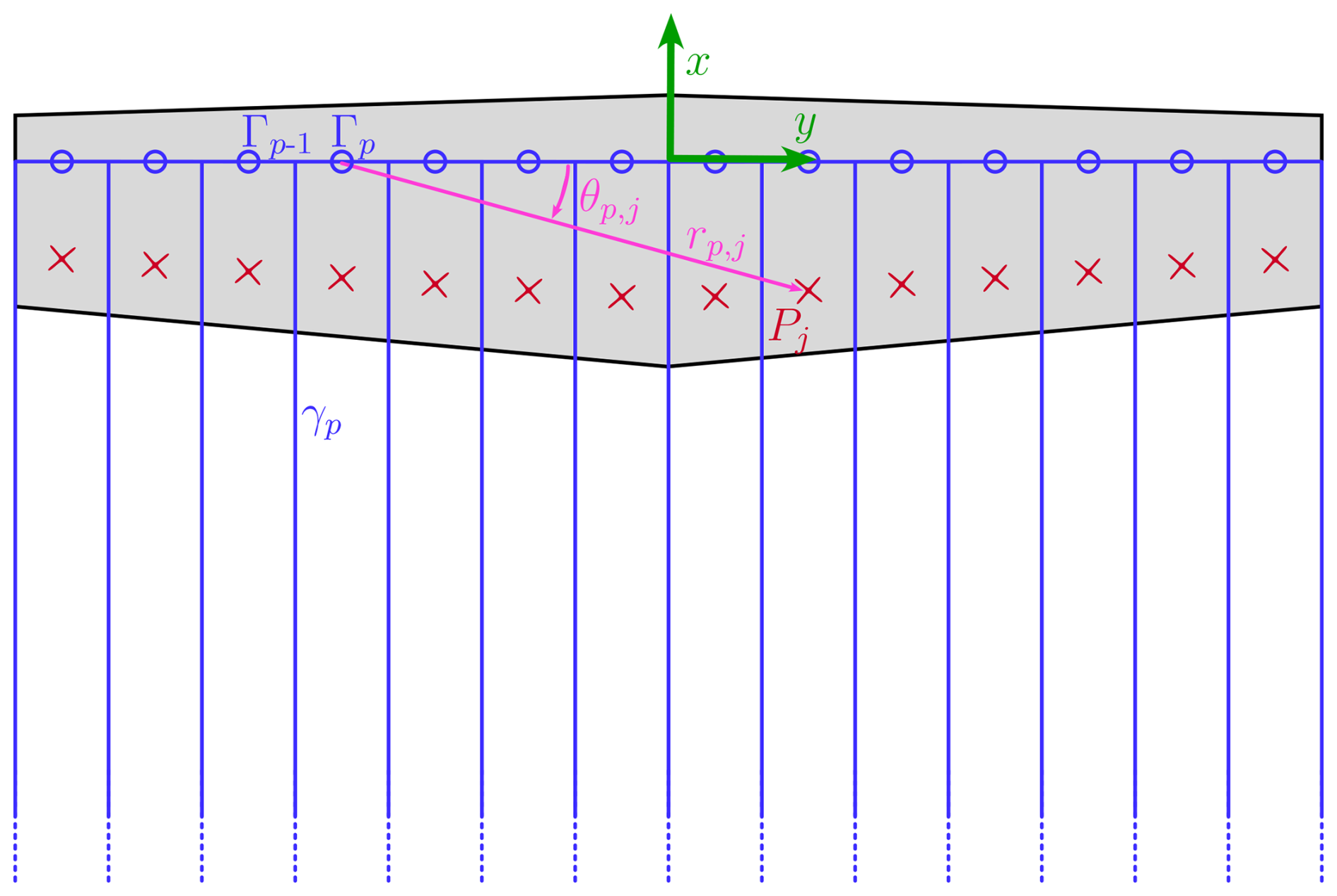
Figure 3 Wing geometry. The bound vorticity Γ_p of the element p and the vorticity ${\mathit{\gamma }}_p={\mathrm{\Gamma }}_p-{\mathrm{\Gamma }}_{p-\mathrm{1}}$ of the trailed vortex p are shown in blue. The red crosses are the evaluation points, with P_j being the evaluation point of element j. The distance r_p,j and the angular position θ_p,j of evaluation point P_j with respect to the start of the vortex filament p are shown in purple.

Since the induced velocities from the three-dimensional vorticity distribution are evaluated at the three-quarter chord point, the induced velocity from the two-dimensional vorticity distribution also needs to be evaluated at the same point (Damiani et al., 2019). The 2D bound vortex induces a velocity at the evaluation point:

$$\begin{array}{}\text{(33)}& \mathrm{\Delta }{w}_j{|}_{\mathrm{2}D}={\displaystyle \frac{{\mathrm{\Gamma }}_j}{\mathrm{2}\mathit{\pi }}}{\displaystyle \frac{\mathrm{1}}{c_j/\mathrm{2}}}.\end{array}$$

The total induced velocity at the evaluation point P_j is then

$$\begin{array}{}\text{(34)}& w_j=\sum _{p=\mathrm{1}}^{N_p}\left(\mathrm{\Delta }{w}_{p,j}{|}_{\mathrm{bound}}\right)+\sum _{p=\mathrm{1}}^{N_p+\mathrm{1}}\left(\mathrm{\Delta }{w}_{p,j}{|}_{\mathrm{trailed}}\right)-\mathrm{\Delta }{w}_j{|}_{\mathrm{2}D}.\end{array}$$

The relative wind velocity at the three-quarter chord point of the aerodynamic section j takes into account the free-stream velocity v_a, as well as the velocities induced by the turbines by the turbines v_t,j and by trailed vorticity w_j:

$$\begin{array}{}\text{(35)}& {\mathit{v}}_{r,j}=\stackrel{{\mathit{v}}_{\mathrm{\infty },j}}{\overbrace{\underset{{\mathit{v}}_a}{\underbrace{-v_{\mathrm{a}}\left[\begin{array}{c}\cos \mathit{\alpha }\\ \mathrm{0}\\ \sin \mathit{\alpha }\end{array}\right]}}+\underset{{\mathit{v}}_{t,j}}{\underbrace{\left[\begin{array}{c}{u}_{t,j}\\ \mathrm{0}\\ w_{t,j}\end{array}\right]}}}}+\left[\begin{array}{c}\mathrm{0}\\ \mathrm{0}\\ w_j\end{array}\right],\end{array}$$

where α is the undisturbed wing angle of attack, defined as the angle between the chord line of the airfoil at the wing center (x direction) and the undisturbed inflow.

The angle of attack used to compute the airfoil lift C_l and drag coefficients C_d is

$$\begin{array}{}\text{(36)}& {\mathit{\alpha }}_{j,\mathrm{3}c/\mathrm{4}}=\arctan \left({\displaystyle \frac{{\mathit{v}}_{r,j}\left(\mathrm{3}\right)}{{\mathit{v}}_{r,j}\left(\mathrm{1}\right)}}\right)+{\mathit{\beta }}_j,\end{array}$$

where β_j is the local twist angle (i.e., the angle between the x direction and the local airfoil chord line), and v_r,j(3) and v_r,j(1) are the third and first elements of the relative wind velocity (Eq. 35).

Figure 4 Angles-of-attack evaluation for an airfoil and sectional lift l_j and drag d_j.

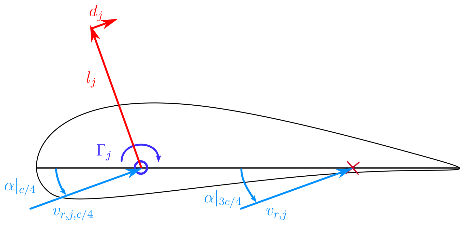
The sectional lift l_j and drag d_j should, however, be projected according to the velocity triangle at the quarter chord lines (Li et al., 2022). The velocity at the quarter-chord line ${\mathit{\alpha }}_{c/\mathrm{4}}$ (${\mathit{P}}_j=[\mathrm{0};y_j;\mathrm{0}]$) takes into account the free-stream velocity v_a, as well as the velocities induced by the turbines v_t,j and by trailed vorticity $w_{j,c/\mathrm{4}}$:

$$\begin{array}{}\text{(37)}& {\mathit{v}}_{r,j,c/\mathrm{4}}=\stackrel{{\mathit{v}}_{\mathrm{\infty },j}}{\overbrace{\underset{{\mathit{v}}_a}{\underbrace{-v_{\mathrm{a}}\left[\begin{array}{c}\cos \mathit{\alpha }\\ \mathrm{0}\\ \sin \mathit{\alpha }\end{array}\right]}}+\underset{{\mathit{v}}_{t,j}}{\underbrace{\left[\begin{array}{c}{u}_{t,j}\\ \mathrm{0}\\ w_{t,j}\end{array}\right]}}}}+\left[\begin{array}{c}\mathrm{0}\\ \mathrm{0}\\ w_{j,c/\mathrm{4}}\end{array}\right].\end{array}$$

The velocity induced by the trailed vorticity is

$$\begin{array}{}\text{(38)}& \begin{array}{rl}{w}_{j,c/\mathrm{4}}& =\sum _{p=\mathrm{1}}^{N_p+\mathrm{1}}{\displaystyle \frac{{\mathit{\gamma }}_p}{\mathrm{4}\mathit{\pi }}}\underset{-\mathrm{\infty }}{\overset{\mathrm{0}}{\int }}{\displaystyle \frac{y_j-y_p}{{r_j}^{\mathrm{3}}}}\mathrm{d}x\\ & =\sum _{p=\mathrm{1}}^{N_p+\mathrm{1}}{\displaystyle \frac{{\mathit{\gamma }}_p}{\mathrm{4}\mathit{\pi }}}{\displaystyle \frac{\mathrm{1}}{y_j-y_p}}.\end{array}\end{array}$$

The angle of attack used to project the lift and drag is then

$$\begin{array}{}\text{(39)}& {\mathit{\alpha }}_{j,c/\mathrm{4}}=\arctan \left({\displaystyle \frac{{\mathit{v}}_{r,j,c/\mathrm{4}}\left(\mathrm{3}\right)}{{\mathit{v}}_{r,j,c/\mathrm{4}}\left(\mathrm{1}\right)}}\right)+{\mathit{\beta }}_j.\end{array}$$

The nonlinear problem formulated to find the induced velocities at each aerodynamic section – and, thus, the aerodynamic coefficients – is solved iteratively by imposing

$$\begin{array}{}\text{(40)}& {\mathrm{\Gamma }}_j{\displaystyle \frac{v_{\mathrm{\infty },j}}{v_{r,j}^{\mathrm{2}}}}={\displaystyle \frac{c_j{C}_{l,j}}{\mathrm{2}}}\end{array}$$

at each evaluation point.

The lift force at each aerodynamic section is

$$\begin{array}{}\text{(41)}& l_j={\displaystyle \frac{\mathrm{1}}{\mathrm{2}}}\mathit{\rho }{c}_j{C}_{l,j}{v}_{r,j}^{\mathrm{2}},\end{array}$$

and the wing lift coefficient is defined as

$$\begin{array}{}\text{(42)}& C_{\mathrm{L}}={\displaystyle \frac{L}{\frac{\mathrm{1}}{\mathrm{2}}\mathit{\rho }A{v}_{\mathrm{a}}^{\mathrm{2}}}}={\displaystyle \frac{{\sum }_{j=\mathrm{1}}^{N_p}{c}_j{C}_{l,j}{v}_{r,j}^{\mathrm{2}}\mathrm{d}{y}_j}{A{v}_{\mathrm{a}}^{\mathrm{2}}}}.\end{array}$$

The integral induced drag D_i can be computed from the induced drag at each wing section d_i,j, which corresponds to the local lift l_j times the local induced angle of attack ${\mathit{\alpha }}_{i,j,c/\mathrm{4}}=\arctan \left(\frac{w_{j,c/\mathrm{4}}}{{\mathit{v}}_{r,j,c/\mathrm{4}}\left(\mathrm{1}\right)}\right)$. The induced drag coefficient is

$$\begin{array}{}\text{(43)}& C_{\mathrm{D},\mathrm{i}}={\displaystyle \frac{D_{\mathrm{i}}}{\frac{\mathrm{1}}{\mathrm{2}}\mathit{\rho }A{v}_{\mathrm{a}}^{\mathrm{2}}}}={\displaystyle \frac{{\sum }_{j=\mathrm{1}}^{N_p}{c}_j{C}_{l,j}{\mathit{\alpha }}_{i,j,c/\mathrm{4}}{v}_{r,j}^{\mathrm{2}}d{y}_j}{A{v}_{\mathrm{a}}^{\mathrm{2}}}}.\end{array}$$

Finally, the three-dimensional profile drag coefficient due to the airfoils C_D,a can be computed as

$$\begin{array}{}\text{(44)}& C_{\mathrm{D},\mathrm{a}}={\displaystyle \frac{{\sum }_{j=\mathrm{1}}^{N_p}{c}_j{C}_{d,j}{v}_{r,j}^{\mathrm{2}}\mathrm{d}{y}_j}{A{v}_{\mathrm{a}}^{\mathrm{2}}}},\end{array}$$

where C_d,j is the airfoil drag coefficient.

2.4 Windplane wake model

To conclude the modeling of the windplane aerodynamics, we need to find how much the wind is slowed down, which means finding the induction a_f in Fig. 2. Trevisi et al. (2023b) show that, for a large turning radius ${\left(\frac{b/\mathrm{2}}{R_{\mathrm{0}}}\right)}^{\mathrm{2}}\ll \mathrm{1}$ and large wing speed ratios $\frac{\mathrm{1}}{{\mathit{\lambda }}^{\mathrm{2}}}\ll \mathrm{1}$, the aerodynamic induction a generated by the helical vortex system (Fig. 5a) can be modeled as the sum of two terms: one due to the first half rotation of the helical vortex filaments (the near-wake induction a_n) and one related to the semi-infinite cascade of vortex rings (the far-wake induction a_f), as in Fig. 5b. The near-wake induction or the near-wake-induced drag D_i can be computed by assuming straight semi-infinite trailed vortices, as carried out in Sect. 2.3.

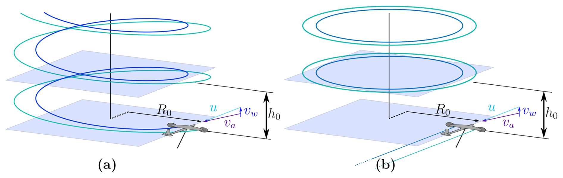
Figure 5 Left and right rolled-up trailed helicoidal vortices (a) and relative modeling after assumptions (b) (Trevisi et al., 2023b).

The far-wake induction a_f can instead be computed by summing up the contribution of each vortex ring. Their strength is equal to the tip vortex strength,

$$\begin{array}{}\text{(45)}& {\mathrm{\Gamma }}_{\mathrm{0}}=\sum _{p=\mathrm{1}}^{N_p/\mathrm{2}+\mathrm{1}}{\mathit{\gamma }}_p,\end{array}$$

and their spanwise position is

$$\begin{array}{}\text{(46)}& y_v={\displaystyle \frac{\mathrm{1}}{{\mathrm{\Gamma }}_{\mathrm{0}}}}\sum _{p=\mathrm{1}}^{N_p/\mathrm{2}+\mathrm{1}}{y}_p{\mathit{\gamma }}_p.\end{array}$$

The wake pitch is

$$\begin{array}{}\text{(47)}& h_{\mathrm{0}}=v_{\mathrm{w}}\left(\mathrm{1}-a_{\mathrm{r}}\right){\displaystyle \frac{\mathrm{2}\mathit{\pi }{R}_{\mathrm{0}}}{u}},\end{array}$$

where v_w(1−a_r) is the axial velocity of the vortex rings. Gaunaa et al. (2020) evaluate the axial velocity of the vortex rings by modeling them as infinite straight vortices and assuming that the dominant effect in the motion of the vortices is the vorticity of the nearest vortex. With this model, tested to be valid by Trevisi et al. (2025), the convection velocity of the rings is

$$\begin{array}{}\text{(48)}& a_{\mathrm{r}}={\displaystyle \frac{\mathrm{1}}{v_w}}{\displaystyle \frac{{\mathrm{\Gamma }}_{\mathrm{0}}}{\mathrm{2}\mathit{\pi }\left(\mathrm{2}{y}_v\right)}}.\end{array}$$

The induction due to the far wake a_f (Fig. 2) can now be evaluated with (Trevisi et al., 2023b)

$$\begin{array}{}\text{(49)}& \begin{array}{rl}{a}_f& ={\displaystyle \frac{\mathrm{1}}{v_{\mathrm{w}}}}{\displaystyle \frac{{\mathrm{\Gamma }}_{\mathrm{0}}}{\mathrm{4}\mathit{\pi }{y}_v}}\sum _{k=\mathrm{1}}^{\mathrm{\infty }}\left({\mathrm{{\rm Y}}}_k\left(-{\mathit{\eta }}_{\mathrm{v}},{\mathit{\lambda }}_{\mathrm{0}}\right)+{\mathrm{{\rm Y}}}_k\left({\mathit{\eta }}_{\mathrm{v}},{\mathit{\lambda }}_{\mathrm{0}}\right)\right)\\ & =a_{\mathrm{r}}\sum _{k=\mathrm{1}}^{\mathrm{\infty }}\left({\mathrm{{\rm Y}}}_k\left(-{\mathit{\eta }}_{\mathrm{v}},{\mathit{\lambda }}_{\mathrm{0}}\right)+{\mathrm{{\rm Y}}}_k\left({\mathit{\eta }}_{\mathrm{v}},{\mathit{\lambda }}_{\mathrm{0}}\right)\right),\end{array}\end{array}$$

where ${\mathit{\eta }}_{\mathrm{v}}=\frac{y_v}{R_{\mathrm{0}}}$ is the tip vortex normalized position, and ${\mathit{\lambda }}_{\mathrm{0}}=\frac{\mathrm{2}\mathit{\pi }{R}_{\mathrm{0}}}{h_{\mathrm{0}}}=\frac{\mathit{\lambda }}{\left(\mathrm{1}-a_{\mathrm{r}}\right)}$ is the normalized torsional parameter of the helicoidal wake. The shape factor Υ_k(η,λ₀) models the induction of one vortex ring and can be computed in closed form as (Trevisi et al., 2023b)

$$\begin{array}{}\text{(50)}& \begin{array}{rl}{\mathrm{{\rm Y}}}_k(\mathit{\eta },{\mathit{\lambda }}_{\mathrm{0}})& ={\displaystyle \frac{-\mathrm{2}\mathit{\eta }}{{\left({\mathit{\eta }}^{\mathrm{2}}+{\left(\frac{\mathrm{2}\mathit{\pi }k}{{\mathit{\lambda }}_{\mathrm{0}}}\right)}^{\mathrm{2}}\right)}^{\mathrm{1}/\mathrm{2}}}}\cdot \\ & \left(F\left(f\right)+{\displaystyle \frac{\mathit{\eta }(\mathit{\eta }-\mathrm{2})-{\left(\frac{\mathrm{2}\mathit{\pi }k}{{\mathit{\lambda }}_{\mathrm{0}}}\right)}^{\mathrm{2}}}{(\mathit{\eta }-\mathrm{2}{)}^{\mathrm{2}}+{\left(\frac{\mathrm{2}\mathit{\pi }k}{{\mathit{\lambda }}_{\mathrm{0}}}\right)}^{\mathrm{2}}}}E\left(f\right)\right),\end{array}\end{array}$$

where F(f) and E(f) are the complete elliptic integral of the first and second kind, respectively, and $f=\frac{\mathrm{4}(\mathit{\eta }-\mathrm{1})}{{\mathit{\eta }}^{\mathrm{2}}+{\left(\frac{\mathrm{2}\mathit{\pi }k}{{\mathit{\lambda }}_{\mathrm{0}}}\right)}^{\mathrm{2}}}$.

3 Windplane aerodynamic design problem

In this section, we formulate the aerodynamic design problem formulation, and we explore the optimal design space. The optimal aerodynamic design problem reads as

$$\begin{array}{}\text{(51)}& \begin{array}{rl}& \underset{\mathit{x}=(a_{\mathrm{f}},\mathbf{\Gamma },\mathit{\alpha },c_{\mathrm{0}},\mathrm{tr},{\mathit{\lambda }}_{\mathrm{t}},K_t)}{max}{C}_P(\mathit{x},\stackrel{\text{parameters: }{\mathrm{\Theta }}_p}{\overbrace{b,m,\underset{\text{turbines}}{\underbrace{N_{\mathrm{bl}},R_{\mathrm{t}\mathrm{0}},R_{\mathrm{t}}}},\underset{\text{tether}}{\underbrace{C_{\mathrm{d},\mathrm{te}},D_{\mathrm{te}},L_{\mathrm{te}}}},\underset{\text{airfoil}}{\underbrace{C_{\mathrm{l}}\left(\mathit{\alpha }\right),C_{\mathrm{d}}\left(\mathit{\alpha }\right)}}}})\\ & \text{subject to:}{h}_{a_{\mathrm{f}}}(\mathit{x},{\mathrm{\Theta }}_p)=\mathrm{0}\mathrm{\text{far wake eq. constraint}}\\ & {\mathit{h}}_{\mathrm{\Gamma }}(\mathit{x},{\mathrm{\Theta }}_p)=\mathbf{0}\mathrm{\text{angles of attack eq. constraints}},\end{array}\end{array}$$

where the optimization variables x are the induction due to the far wake a_f; the bound circulation at each wing aerodynamic section Γ; the wing angle of attack α; the chord at the wing center c₀, the taper ratio of the trapezoidal wing tr; the onboard turbine tip speed ratio λ_t; and the parameter K_t, determining the radial distribution of k(r_t) (see Sect. 2.2).

The induction due to the far wake a_f is settled by the optimizer to satisfy $h_{a_{\mathrm{f}}}(\mathit{x},{\mathrm{\Theta }}_p)=\mathrm{0}$ (Eq. 49), and the bound circulation at each aerodynamic section Γ_j is settled to satisfy ${\mathit{h}}_{\mathrm{\Gamma }}(\mathit{x},{\mathrm{\Theta }}_p)=\mathbf{0}$ (Eq. 40).

The objective function is the power coefficient C_P (Eq. 15). Optimizing for this power coefficient is equivalent to optimizing for the shaft power while keeping the wing span constant.

A trapezoidal wing with constant twist is analyzed here. Future studies will investigate the influence of different wing shapes and twist distributions on the system performances. In particular, understanding the optimal lift distribution for a windplane, considering the far wake and the onboard wind turbines, is expected to increase the power production further. The onboard turbines are conceptually designed by modifying their tip speed ratio λ_t and the parameter K_t. The radial distribution of the parameter k(r_t) (see Sect. 2.2) is assumed to be parabolic and a function of K_t as follows:

$$\begin{array}{}\text{(52)}& k\left(r_t\right)=K_t-{\displaystyle \frac{\mathrm{4}{K}_t}{(R_{\mathrm{t}}-R_{\mathrm{t}\mathrm{0}}{)}^{\mathrm{2}}}}{\left(r_t-{\displaystyle \frac{(R_{\mathrm{t}}+R_{\mathrm{t}\mathrm{0}})}{\mathrm{2}}}\right)}^{\mathrm{2}},\end{array}$$

where R_t is the turbine radius, and R_t0 is the hub radius. Future studies will investigate the effect of different loading shapes (i.e., different distributions of the parameter k(r_t)) on the system performances.

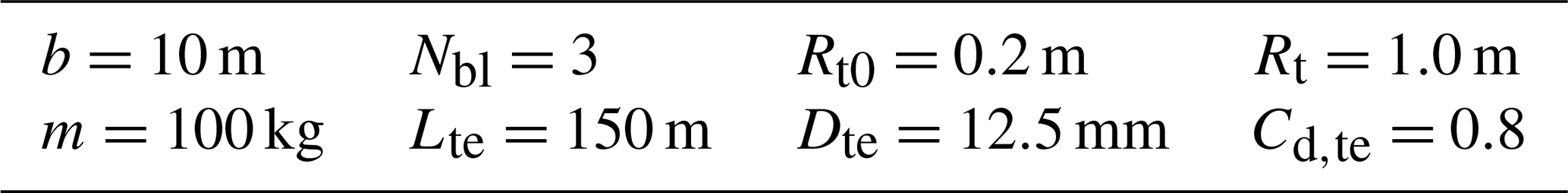
The other fixed parameters are the wing span b, the system mass m, the number of turbine blades N_bl, the tether section drag coefficient C_d,te, the tether diameter D_te, the tether length L_te, and the airfoil polars as a function of the angle of attack (C_l(α),C_d(α)).

By solving this optimization problem, we can get to a design of the wing and of the turbines. To get to the chord and twist of the turbine blades, the Glauert tip correction is applied (Branlard, 2017)⁴. The turbine design features a constant lift coefficient along the blade span at the design tip speed ratio. In order to achieve a realistic design, the design lift coefficient at the blade tip is lowered to delay stall at lower tip speed ratios, and the chord at the blade root is increased to allow for the hub connection. For these reasons, the chord at the root and at the tip is slightly widened, while the twist is adjusted to keep the same lift force.

Design space exploration

We first explore the optimal design space to study the influence of the turbine position and of the airfoil characteristics on the power output. We chose the parameters in Table 1, which are slightly adjusted with respect to the analyses by Trevisi (2024). The wing is discretized into 100 elements of constant size. The optimization problem (51) is solved in MATLAB with the sequential quadratic programming algorithm implemented in the function fmincon. The solution of the problem takes a few tens of seconds on a standard laptop. Local minima, which are not interesting for this application, can be found when the solver finds solutions with an angle of attack above stall.

Table 1 Parameters for the optimal design problem.

For this study, we compared three turbines' positions (Fig. 6):

• a.

  Turbines rotating inboard down, located at one rotor hub radius outward from the wing tip ($y_{\mathrm{t}}=\pm \left(\frac{b}{\mathrm{2}}+R_{\mathrm{t}\mathrm{0}}\right)=\pm \mathrm{5.2}$ m) (indicated with continuous lines in Figs. 7 to 15).

• b.

  Turbines rotating inboard down, located in front of the wing ($y_{\mathrm{t}}=\pm \frac{b}{\mathrm{4}}=\pm \mathrm{2.5}$ m) (indicated with dashed lines in Figs. 7 to 15).

• c.

  Turbines mounted on pylons (indicated with dotted lines from Figs. 7 to Fig. 15). To model this case, we switch off the interactional aerodynamics between the turbines and the wing while neglecting the parasite drag associated with the pylons. A detailed analysis of the effect of the vertical rotor position on the wing aerodynamics is given by Mehr et al. (2024).

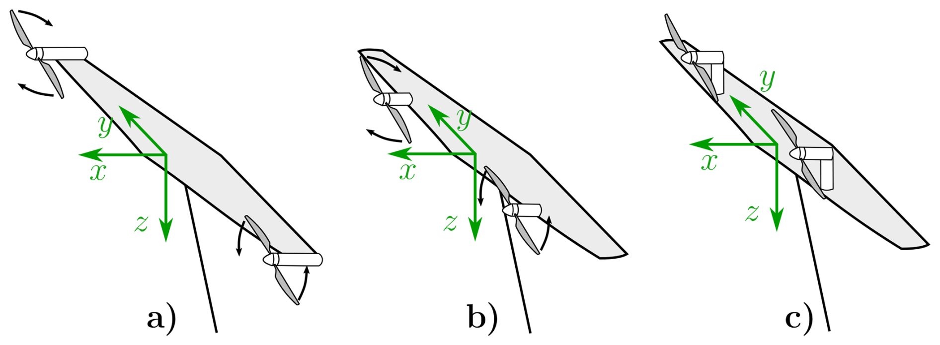
Figure 6 Representation of the three windplane layouts considered for the design space exploration study.

Moreover, we consider idealized airfoils on the windplane wing. This is to study the influence of their key metrics on the resulting design. The idealized airfoils have prescribed maximum efficiency $E_{\mathrm{a},\max }=\frac{C_{\mathrm{l}}}{C_{\mathrm{d}}}{|}_{\max }=[\mathrm{75},\mathrm{100},\mathrm{125}]$ at different lift coefficients $C_{\mathrm{l}}{|}_{E_{\mathrm{a},\max }}$. The airfoil lift coefficient is modeled to vary linearly with respect to the angle of attack as $C_{\mathrm{l}}=\mathrm{2}\mathit{\pi }\mathit{\alpha }+\mathrm{0.3}$, and the efficiency E_a is modeled as a parabola $E_{\mathrm{a}}=E_{\mathrm{a},\max }-e_{\mathrm{2},a}{\left(\left(\mathit{\alpha }-\mathit{\alpha }{|}_{E_{\mathrm{a},\max }}\right)\frac{\mathrm{180}}{\mathit{\pi }}\right)}^{\mathrm{2}}$, with the peak being equal to E_a,max, achieved at the angle of attack $\mathit{\alpha }{|}_{E_{\mathrm{a},\max }}$ and at the lift coefficient $C_{\mathrm{l}}{|}_{E_{\mathrm{a},\max }}$⁵.

Figure 7 shows the wing lift coefficient C_L as a function of the airfoil lift coefficient of maximum efficiency $C_{\mathrm{l}}{|}_{E_{\mathrm{a},\max }}$. Recall that the data in the figure represent the solutions of the optimization problem (51). The trends show that it is optimal to design the wing such that it operates the airfoils at their maximum efficiency.

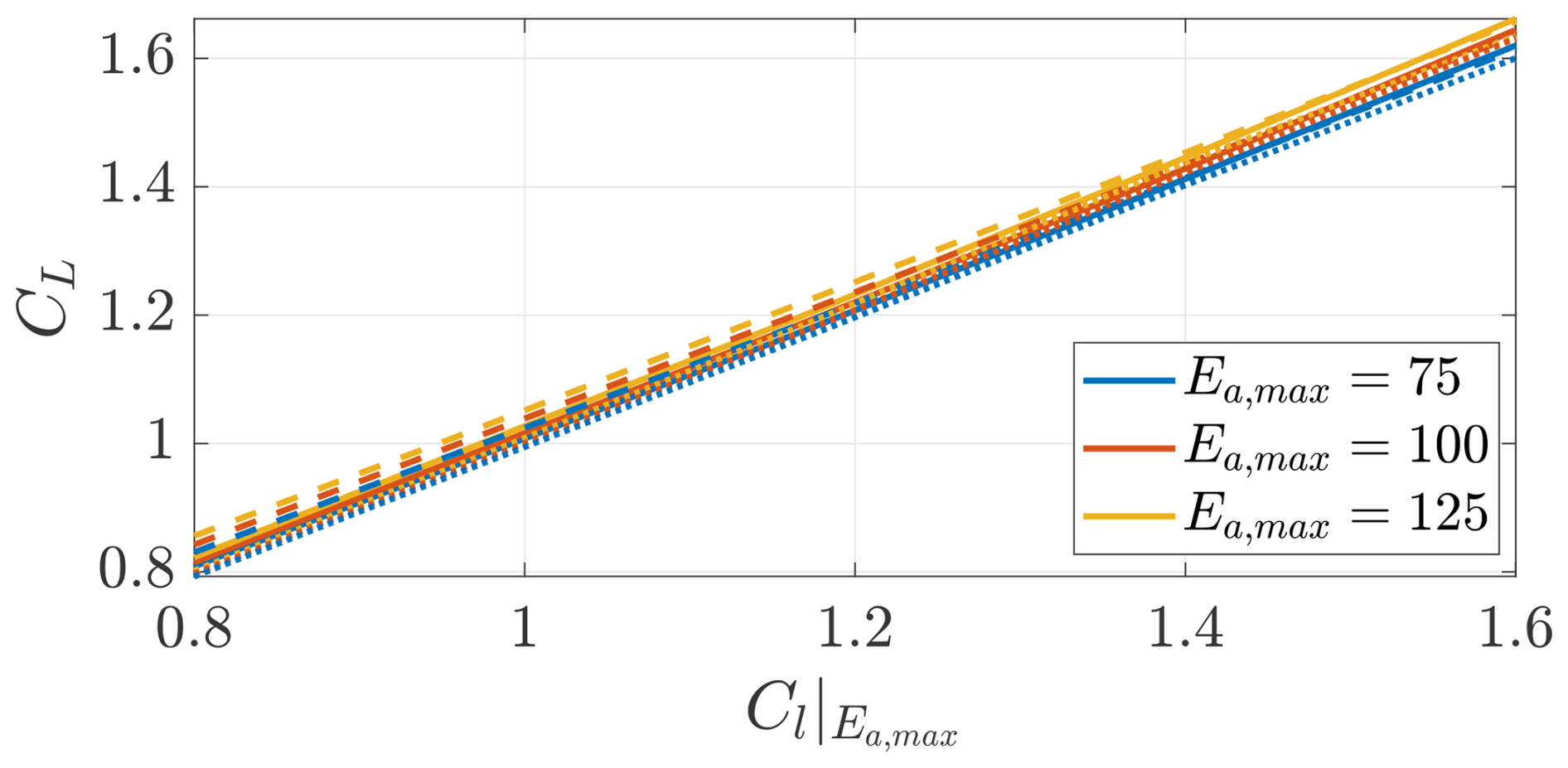
Figure 7 Optimal wing lift coefficient as a function of the lift coefficient of maximum airfoil efficiency $C_{\mathrm{l}}{|}_{E_{\mathrm{a},\max }}$. Trends shown for three different values of maximum airfoil efficiency E_a,max and for three turbines' positions (on the pylons ($\cdot \cdot \cdot$), in front of the wing ($--$), and on the wing tip (−)).

Figure 8 shows the optimal aspect ratio AR as a function of the airfoil lift coefficient of maximum efficiency $C_{\mathrm{l}}{|}_{E_{\mathrm{a},\max }}$. The aspect ratio has a similar physical meaning to the solidity of conventional turbines. For increasing $C_{\mathrm{l}}{|}_{E_{\mathrm{a},\max }}$, increasing aspect ratios are optimal. The optimal aspect ratio is almost insensible to the airfoil maximum efficiency E_a,max and to the interactional aerodynamics.

The trends in Figs. 7 and 8 are a direct consequence of the optimization objective function, i.e., the power coefficient defined in Eq. (15). This power coefficient informs us about the power for a given wingspan. Similarly, the power coefficient of conventional wind turbines informs us about the power for a given blade span. Conventional wind turbines are designed such that the airfoils along the blade span operate at their maximum efficiency. The chord radial distribution (i.e., the solidity) is settled such that the radial distribution of the induction is optimal, subsequently maximizing the power production (Manwell et al., 2009). Similarly, windplanes optimizing this power coefficient are designed such that the airfoils operate at their maximum efficiency. The chord distribution (i.e., the aspect ratio) is settled such that the induced velocities (or the induced drag) are optimal, subsequently maximizing the power production. Airborne wind energy systems in the literature are designed to maximize the power per a given wing area or, equivalently, the power-harvesting factor ξ_P (Fasel et al., 2017; Bauer et al., 2018; Echeverri et al., 2020a; Trevisi et al., 2021 among others), which be written as

$$\begin{array}{}\text{(53)}& {\mathit{\xi }}_{\mathrm{p}}={\displaystyle \frac{P}{\frac{\mathrm{1}}{\mathrm{2}}\mathit{\rho }A{v}_{\mathrm{w}}^{\mathrm{3}}}}=\mathit{\pi }\mathrm{AR}{C}_{\mathrm{P}},\end{array}$$

where the wing area is $A=\frac{b^{\mathrm{2}}}{\mathrm{AR}}$. Wings designed to maximize ξ_p have an high aspect ratio and operate at the angle of attack which maximizes the metric $\frac{C_{\mathrm{L}}^{\mathrm{3}}}{C_{\mathrm{D}}^{\mathrm{2}}}$, which is achieved, in practice, at the highest lift coefficient. The airfoils are then designed to maximize the metric $\frac{C_{\mathrm{l}}^{\mathrm{3}}}{C_{\mathrm{d}}^{\mathrm{2}}}$ (Bauer et al., 2018; De Fezza and Barber, 2022; Porta Ko et al., 2023; Rangriz and Kheiri, 2025, among others). The most meaningful objective among the two is the one leading to the lowest levelized cost of energy. The cost of energy of windplanes is expected to increase with the structural material mass, which scales with the cube of the wingspan b³ (Sommerfeld et al., 2022). Therefore, taking the objective as a function of the wingspan (i.e., the power coefficient) is expected to be aligned with a cost-oriented objective. The influence of the two design objectives on the aerodynamic design was first analyzed by Trevisi (2024), and the main conclusions are confirmed here.

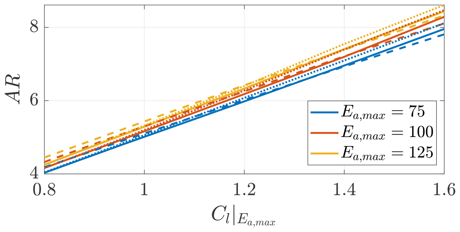
Figure 8 Optimal wing aspect ratio as a function of the lift coefficient of maximum airfoil efficiency $C_{\mathrm{l}}{|}_{E_{\mathrm{a},\max }}$. Trends shown for three different values of maximum airfoil efficiency E_a,max and for three turbines' positions (on pylons ($\cdot \cdot \cdot$), in front of the wing ($--$), and on the wing tip (−)).

Figures 9 and 10 show the onboard turbine tip speed ratio λ_t and the turbines' power coefficient C_P,t. Recall that the onboard turbines are designed to maximize the windplane power coefficient C_P (Eq. 15) and not their own power coefficients C_P,t. Considering the interactional aerodynamics, the optimal tip speed ratio decreases to increase the wake swirl and, thus, to increase the change in inflow angle, reducing the induced drag of the wing aerodynamic sections behind the rotors. With the turbines placed at the wing tips, the tip speed ratio is the lowest. Designs with lower tip speed ratios and, thus, lower angular velocities are typically preferable to reduce the noise emission (Chirico et al., 2018).

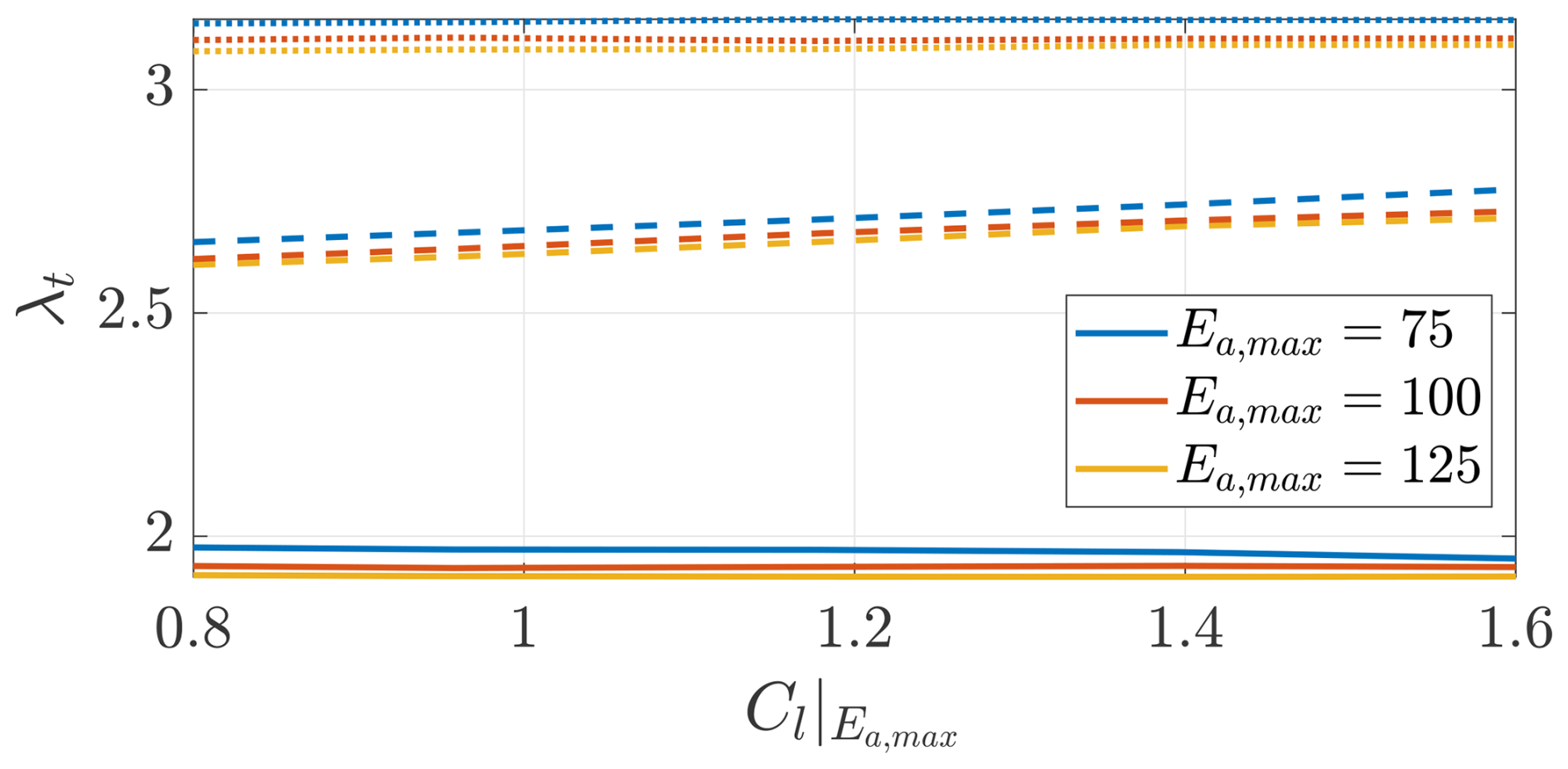
Figure 9 Optimal onboard turbines' tip speed ratios as a function of the lift coefficient of maximum airfoil efficiency $C_{\mathrm{l}}{|}_{E_{\mathrm{a},\max }}$. Trends shown for three different values of maximum airfoil efficiency E_a,max and for three turbines' positions (on pylons ($\cdot \cdot \cdot$), in front of the wing ($--$), and on the wing tip (−)).

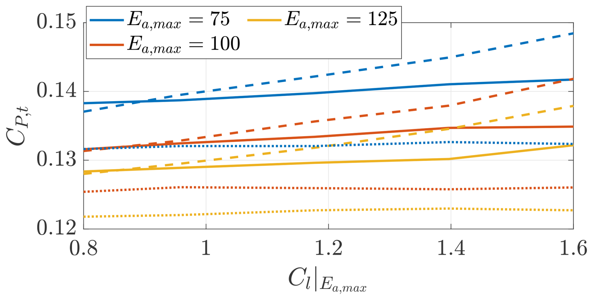
Figure 10 Optimal onboard turbine power coefficient as a function of the lift coefficient of maximum airfoil efficiency $C_{\mathrm{l}}{|}_{E_{\mathrm{a},\max }}$. Trends shown for three different values of maximum airfoil efficiency E_a,max and three turbines' positions (on pylons ($\cdot \cdot \cdot$), in front of the wing ($--$), and on the wing tip (−)).

Figure 11 shows the ratio between the lift coefficient and the system drag coefficient. The designs with the turbines at the wing tips achieve the highest $C_{\mathrm{L}}/C_{\mathrm{D}}$ because of the turbines effectively reducing the induced drag. Figure 12 shows the ratio between the thrust force T_t and the total wind plane drag D_p+D_i. Loyd (1980) shows that, for idealized turbines, the optimal ratio between the turbines' thrust and the total drag is 0.5. The values found in this study confirm this finding, even with a more detailed wind turbine model. For the case with the turbines placed on the pylons, the ratio between the turbines' thrust and drag is slightly lower.

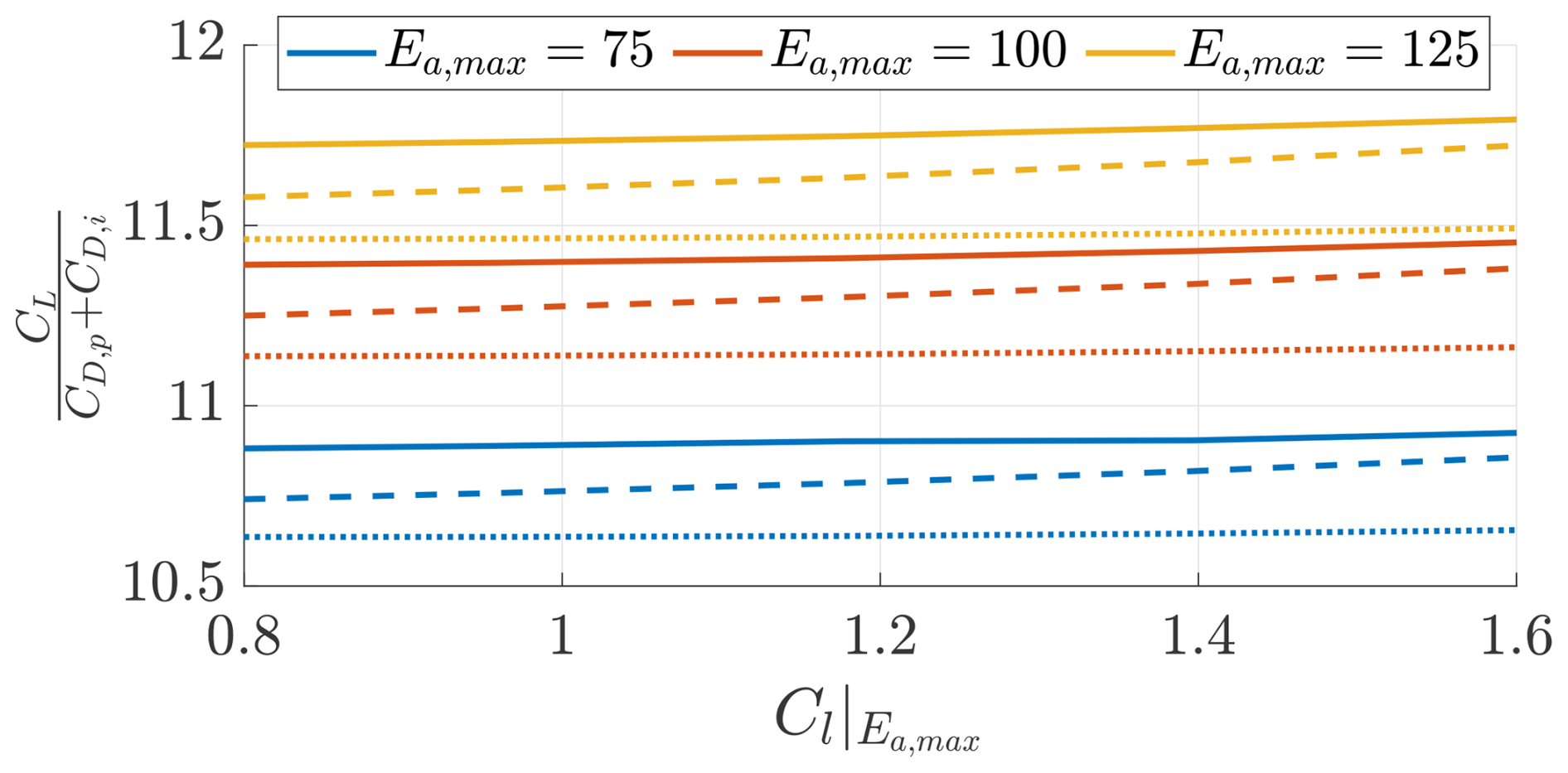
Figure 11 Ratio between the wing lift coefficient C_L and total drag coefficient $C_{D,p}+C_{\mathrm{D},\mathrm{i}}$. Trends shown for three different values of maximum airfoil efficiency E_a,max and for three turbines' positions (on pylons ($\cdot \cdot \cdot$), in front of the wing ($--$), and on the wing tip (−)).

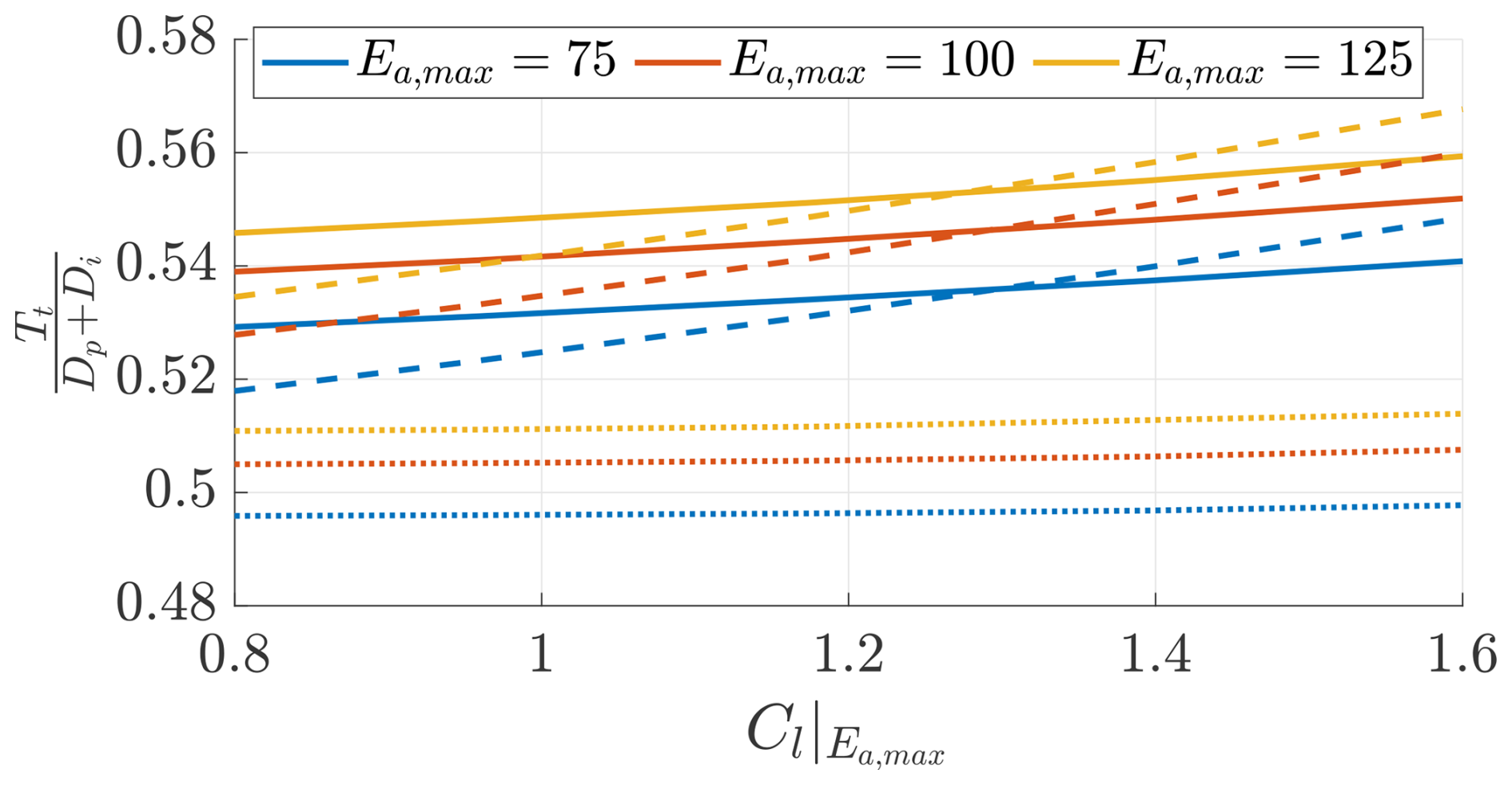
Figure 12 Ratio between the onboard turbine thrust force T_t and total drag force D_p+D_in. Trends shown for three different values of maximum airfoil efficiency E_a,max and three turbines' positions (on pylons ($\cdot \cdot \cdot$), in front of the wing ($--$), and on the wing tip (−)).

Figure 13 shows the wing speed ratios for the analyzed cases. The windplane flies slightly slower when the turbines are placed in front of the wing. The wing speed ratio is strictly related to the $C_{\mathrm{L}}/C_{\mathrm{D}}$ (Fig. 11), but it includes the effect of the turbine thrust and of the far-wake induction (Eq. 13). Recall that the windplane power coefficient C_P (Eq. 15) is a function of the onboard turbines' power coefficient C_P,t and of the cube of the wing speed ratio λ³.

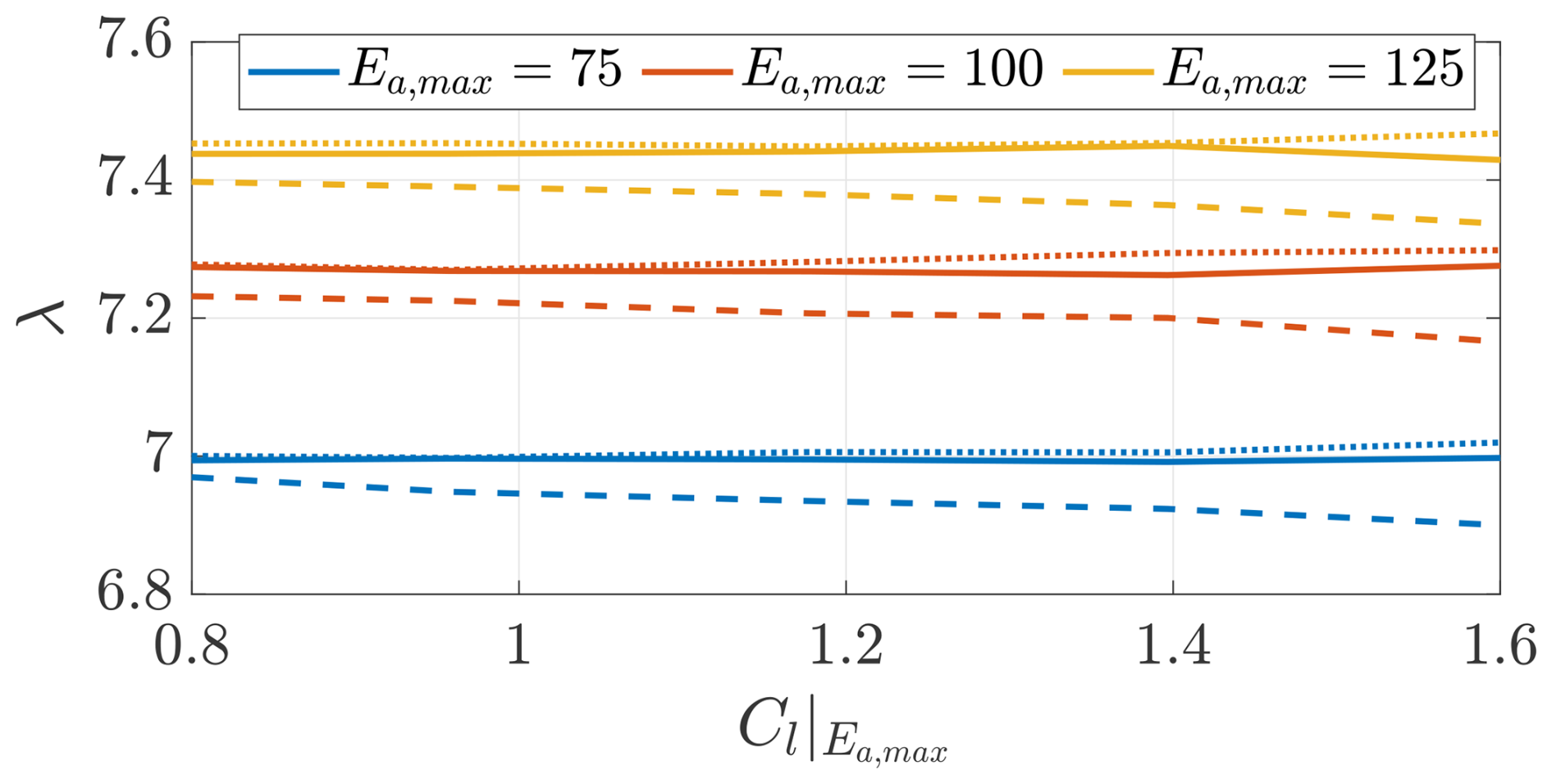
Figure 13 Optimal windplane wing speed ratio as a function of the lift coefficient of maximum airfoil efficiency $C_{\mathrm{l}}{|}_{E_{\mathrm{a},\max }}$. Trends shown for three different values of maximum airfoil efficiency E_a,max and for three turbines' positions (on pylons ($\cdot \cdot \cdot$), in front of the wing ($--$), and on the wing tip (−)).

Figure 14 shows the optimal taper ratio as a function of the airfoil lift coefficient of maximum efficiency $C_{\mathrm{l}}{|}_{E_{\mathrm{a},\max }}$. Higher taper ratios are preferable if the turbines are placed at the wing tips. This is because higher taper ratio wings have more lifting area behind the turbines, enhancing their beneficial effect on the power production.

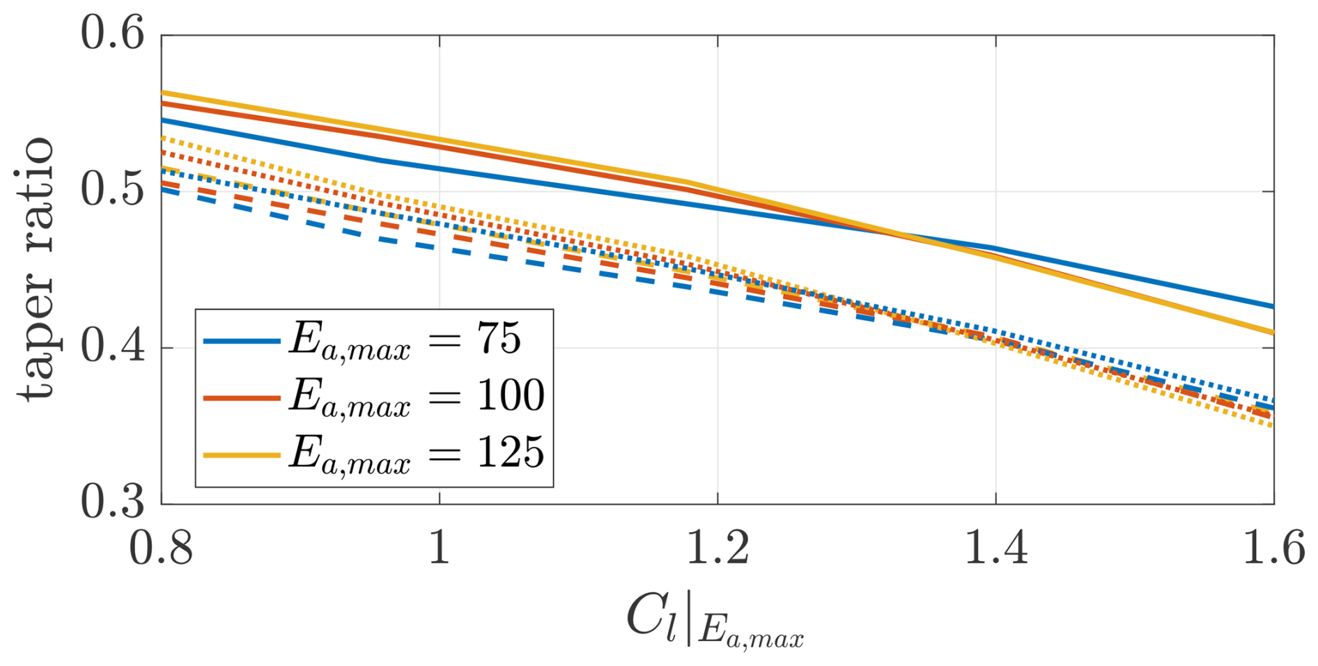
Figure 14 Optimal taper ratio as a function of the lift coefficient of maximum airfoil efficiency $C_{\mathrm{l}}{|}_{E_{\mathrm{a},\max }}$. Trends shown for three different values of maximum airfoil efficiency E_a,max and three turbines position (on pylons ($\cdot \cdot \cdot$), in front of the wing ($--$), and on the wing tip (−)).

Figure 15 shows the optimal power coefficient C_P as a function of the airfoil lift coefficient of maximum efficiency $C_{\mathrm{l}}{|}_{E_{\mathrm{a},\max }}$. The power coefficient is sensitive to the maximum airfoil efficiency E_a,max and slightly sensitive to $C_{\mathrm{l}}{|}_{E_{\mathrm{a},\max }}$. Indeed, larger power coefficients can be achieved with more efficient airfoils. Moreover, the position of the turbines influences the power production. If they are placed on pylons, the power is the lowest even if the parasite drag associated with the pylons is neglected.

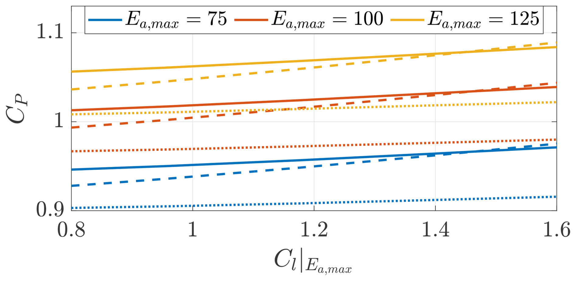
Figure 15 Optimal power coefficient as a function of the lift coefficient of maximum airfoil efficiency $C_{\mathrm{l}}{|}_{E_{\mathrm{a},\max }}$. Trends shown for three different values of maximum airfoil efficiency E_a,max and three turbines' positions (on pylons ($\cdot \cdot \cdot$), in front of the wing ($--$), and on the wing tip (−)).

Placing the turbines at the wing tips improves the power production compared to placing them in front of the wing. Note that the turbines rotate inboard down. This can also be seen in Fig. 16, where the position of the turbines y_t is moved along the wing for three different values of maximum airfoil efficiency E_a,max with $C_{\mathrm{l}}{|}_{E_{\mathrm{a},\max }}=\mathrm{1}$. If the turbines are placed in front of the wing, the wing sections placed inward from the turbine position experience a beneficial change in inflow angle, while the wing sections placed outward experience a disadvantageous change in inflow angle. If the turbines are placed at the wing tips, there are no wing sections outward from the turbine position so that only the beneficial effects in the inward wing sections are experienced. Since the nacelle is not modeled in this study, the portion of wing behind the rotor hub position sees a slight increase in inflow speed. For this reason, the peak in C_P corresponds to one rotor hub diameter inward. The peak in real systems will be influenced by the presence of the nacelle and the associated parasite drag, and so the exact position and amplitude of this peak will change consequently. With the turbines getting closer to the wing tip, the interactional aerodynamics become more beneficial for the power production, and, thus, it is optimal for the onboard turbines to increase their wake swirl. For this reason, the optimal onboard turbines' tip speed ratio decreases for the turbines getting closer to the tip, as shown in Fig. 17. To shed light on how big the beneficial interaction is, the figures also show the effect of rotating the turbines in the non-beneficial outboard down direction, where a significant drop in the power coefficient can be observed.

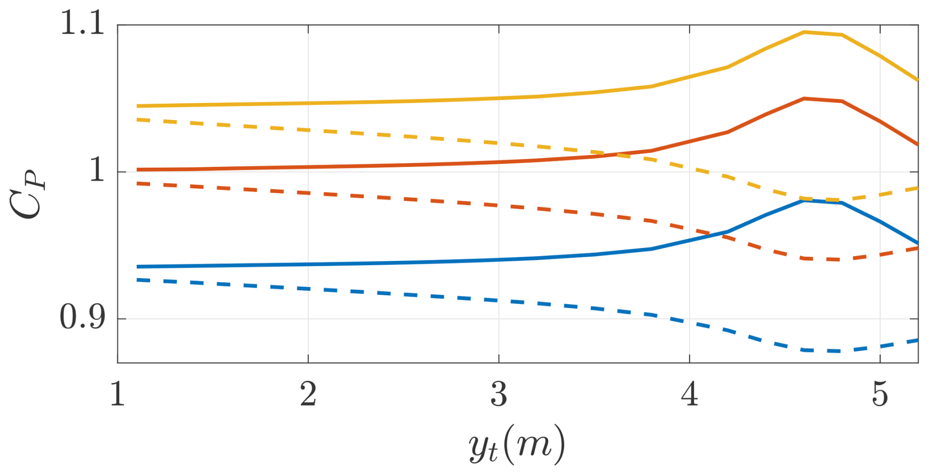
Figure 16 Optimal power coefficient as a function of the spanwise position of the turbines for rotation direction inboard down (−) and outboard down ($--$). Trends shown for three different values of maximum airfoil efficiency E_a,max with $C_{\mathrm{l}}{|}_{E_{\mathrm{a},\max }}=\mathrm{1}$.

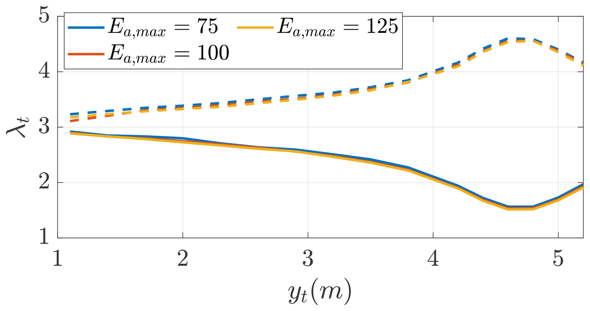
Figure 17 Optimal onboard turbine tip speed ratio as a function of the spanwise position of the turbines for rotation direction inboard down (−) and outboard down ($--$). Trends shown for three different values of maximum airfoil efficiency E_a,max with $C_{\mathrm{l}}{|}_{E_{\mathrm{a},\max }}=\mathrm{1}$.

As a final study, the optimal designs are studied as a function of the onboard turbines' radius. Figure 18 shows the optimal power coefficient as a function of the turbines' radius. The power increases for larger radius, such that the turbines can operate at higher $C_{\mathrm{P},\mathrm{t}}/C_{\mathrm{T},\mathrm{t}}$ (Fig. 19). Higher $C_{\mathrm{P},\mathrm{t}}/C_{\mathrm{T},\mathrm{t}}$ values indicate that less power is lost in the conversion from thrust power (i.e., the power experienced by the windplane dynamics) to generated power (i.e., the power experienced by the turbines' shaft). When the turbines are placed at the wing tips, a lower $C_{\mathrm{P},\mathrm{t}}/C_{\mathrm{T},\mathrm{t}}$ is optimal because of the beneficial effects of the interactional aerodynamics. From an aerodynamic point of view, the turbines' radius should be as large as possible. However, the final turbine size will be determined by including structural, electrical, and control considerations. In this study, we keep the turbine radius fixed to R_t=1 m, which seems to be reasonable because the power coefficient is approaching the plateau.

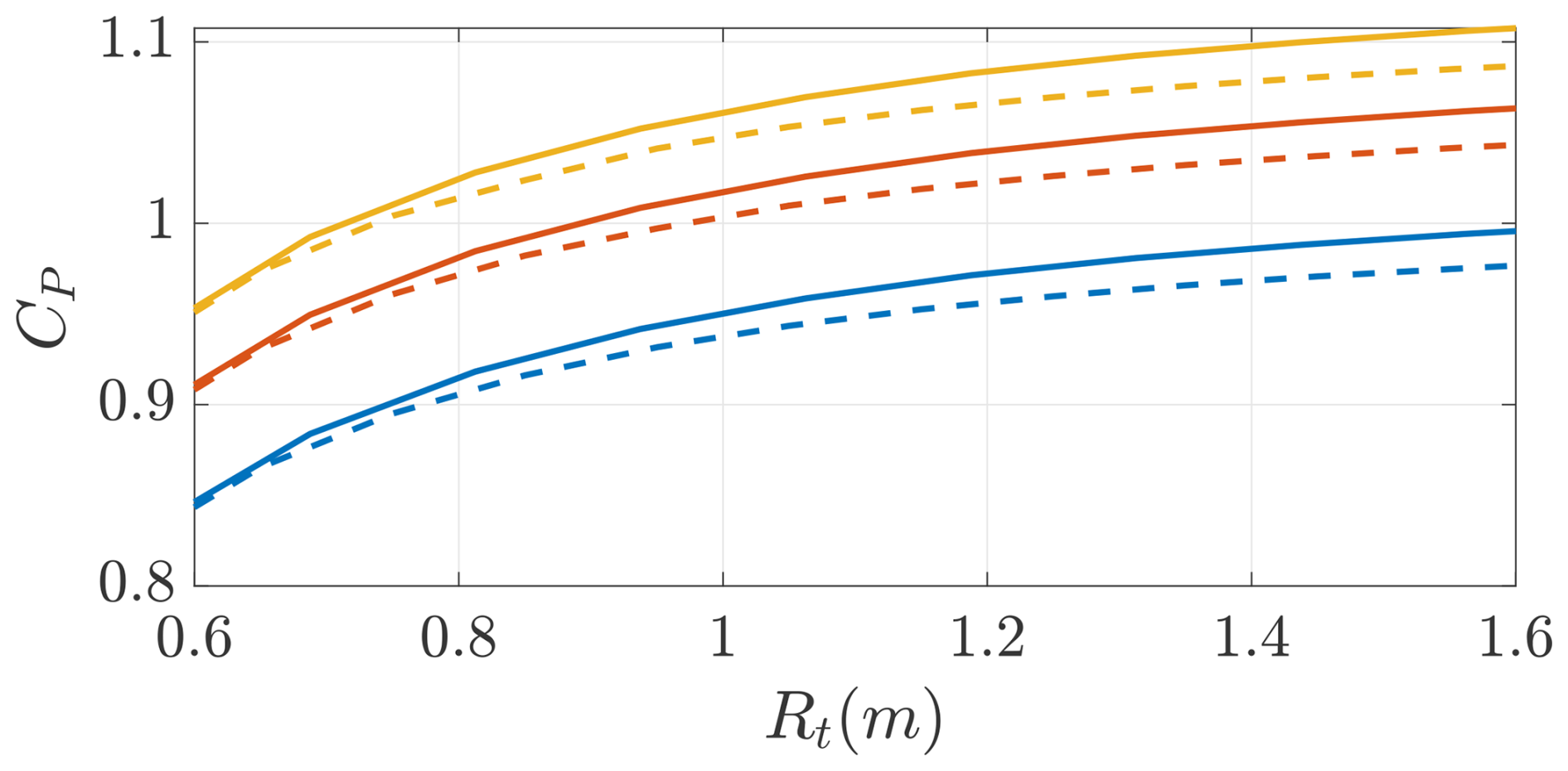
Figure 18 Optimal power coefficient as a function of the onboard turbines' radius R_t for two turbines' positions (in front of the wing ($--$) and on the wing tip (−)). Trends shown for three different values of maximum airfoil efficiency E_a,max with $C_{\mathrm{l}}{|}_{E_{\mathrm{a},\max }}=\mathrm{1}$.

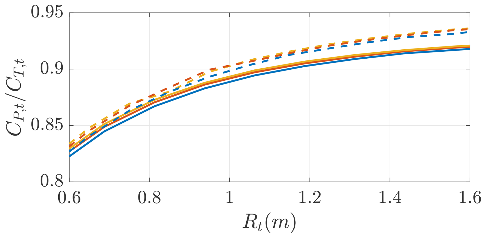
Figure 19 Onboard turbines $C_{\mathrm{P},\mathrm{t}}/C_{\mathrm{T},\mathrm{t}}$ as a function of the onboard turbines' radius R_t for two turbines' positions (in front of the wing ($--$) and on the wing tip (−)). Trends shown for three different values of maximum airfoil efficiency E_a,max with $C_{\mathrm{l}}{|}_{E_{\mathrm{a},\max }}=\mathrm{1}$.

To conclude, this study shows that conventional efficient airfoils should be used in the design of windplanes and that the optimal aspect ratio is finite. The windplane should then be designed such that it operates at the lift coefficient corresponding to the airfoil maximum efficiency. The optimal wing taper ratio and the optimal onboard turbines' tip speed ratios are influenced by the interactional aerodynamics. If the turbines are placed at the wing tips and the windplane is designed accordingly, the power can increase considerably (approx 5 %).

4 Vortex particle method: DUST

To validate our analytical results, we use DUST⁶, an open-source aerodynamic simulation software that employs the vortex particle method (Cottet and Koumoutsakos, 2000). This grid-free Lagrangian approach effectively models free wake vorticity evolution and has been developed in accordance with modern FORTRAN standards. It incorporates classical potential-based aerodynamic models, including the lifting-line method (Gallay and Laurendeau, 2015; Piszkin and Levinsky, 1976), surface panels (Piszkin and Levinsky, 1976), and vortex lattice elements (Katz and Plotkin, 2001). While the software assumes incompressible potential flow, compressibility effects are accounted for using the Prandtl–Glauert correction in steady aerodynamic load computations. Additionally, lifting-line and vortex lattice elements incorporate both compressibility and viscous effects through Mach-dependent aerodynamic coefficient tables.

We select the lifting-line element to model the turbine blades because it eliminates the need for explicitly modeling the surface mesh as the flow particles do not interact directly with the blade surface. For the wing, using a lifting-line element can pose challenges in detecting the penetration condition (Niro et al., 2024). Therefore, we opt for the vortex lattice element as it provides accurate results without the higher computational cost associated with surface panel elements.

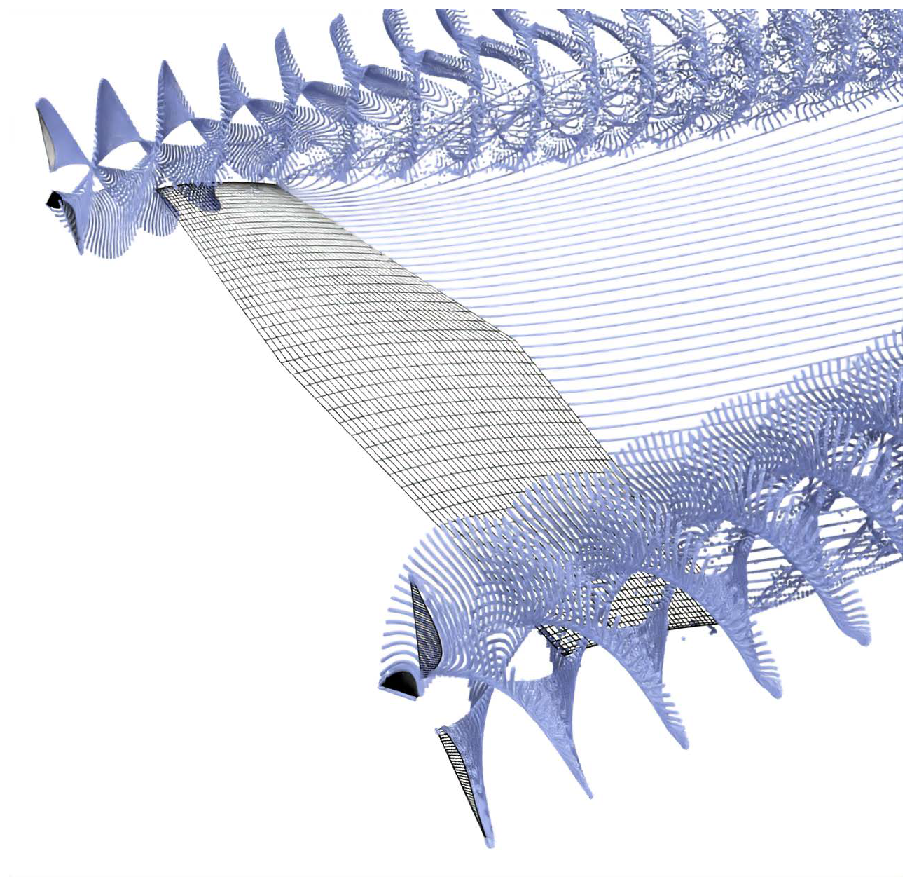
Figure 20 shows the DUST setup for this simulation. The blue dots represent the vortex particles trailed by the lifting surfaces.

Figure 20 Visualization of the DUST simulations. The blue dots are the vortex particles.

5 Optimal aerodynamic design

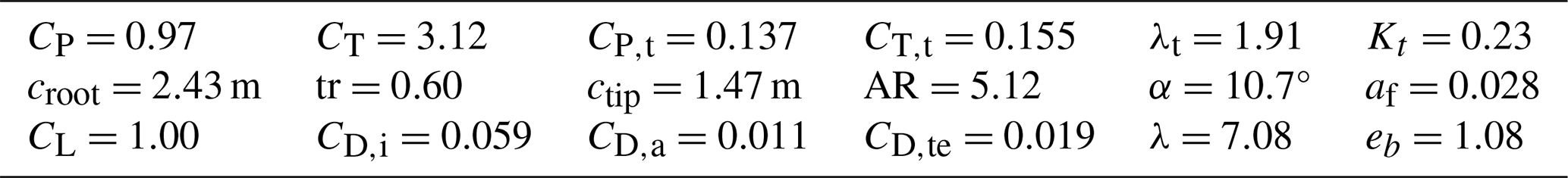
In this section, we present the optimal design and analyze it with DUST. The main inputs for this case study are given in Table 1. The 10 m wingspan windplane was initially designed by Trevisi (2024), and its design is refined here. The NACA4421 airfoils are used for both the wing and the onboard turbines. The chord-based Reynolds number for the wing is above 1×10⁶, while the turbine blades have a chord-based Reynolds number between 200 000 and 500 000. The dependence of the airfoils polars on the Reynolds number can be taken into account in DUST by providing the polars for different Reynolds numbers. This airfoil is chosen because it has a high maximum efficiency $E_{\mathrm{a},\max }=\mathrm{103}$ (Re=10⁶) at a lift coefficient of $C_{\mathrm{l}}{|}_{E_{\mathrm{a},\max }}=\mathrm{1.01}$, with a relatively large thickness (21 %), which is good for the structural design.

The main optimization results are reported in Table 2. The wing is discretized into 60 elements with a cosine distribution to refine the discretizations after the turbines. The windplane achieves a power coefficient of C_P=0.97. The turbines operate with a low tip speed ratio of λ_t=1.91. Lowering the tip speed ratio increases the wake swirl and thus the inflow angle at the wing sections after the turbines. This low value of λ_t is also good to limit the acoustic emission (Chirico et al., 2018). The wing has a low aspect ratio of AR=5.1, which is good for structural design and maneuverability, has a taper ratio of tr=0.60 and operates at the maximum efficiency lift coefficient C_L=1.00, leading to a wing speed ratio of λ = 7.08. The main drag component is the induced drag, accounting for 66.3 % of the total drag, followed by the tether drag with 21.3 % and by the airfoil drag with 12.4 %. While the breakdown of the drag components is case-dependent, the ratio between the total turbines' thrust and the aerodynamic drag is 56.1 %, similarly to the values in Fig. 12 and to the optimal value of 50 % found by Loyd (1980). The spanwise efficiency e_b indicates how efficiently the wing generates lift with respect to the induced drag (Anderson, 2017). It can be estimated as

$$\begin{array}{}\text{(54)}& e_b={\displaystyle \frac{C_{\mathrm{L}}^{\mathrm{2}}}{\mathit{\pi }\mathrm{AR}{C}_{\mathrm{D},\mathrm{i}}}}.\end{array}$$

Modeling the wing with Prandtl lifting-line theory, which is accurate for high aspect ratios, the spanwise efficiency for an isolated wing with an elliptic lift distribution is e_b=1. Modeling the wing with the present formulation is accurate even for a low-aspect-ratio wing because the effects of the 2D bound circulation are considered. When accounting for the onboard turbine's influence on the wing, the spanwise efficiency can take values above 1. This value is then representative of the effects of the onboard wind turbines on the wing-induced drag. Note that the spanwise efficiency e_b should not be confused with the Oswald efficiency, which also accounts for the parasite drag components of the windplane (Anderson, 2017; Trevisi, 2024) and the induced drag produced by other lifting surfaces on the windplane (e.g., stabilizers).

Table 2 Main aerodynamic optimization results.

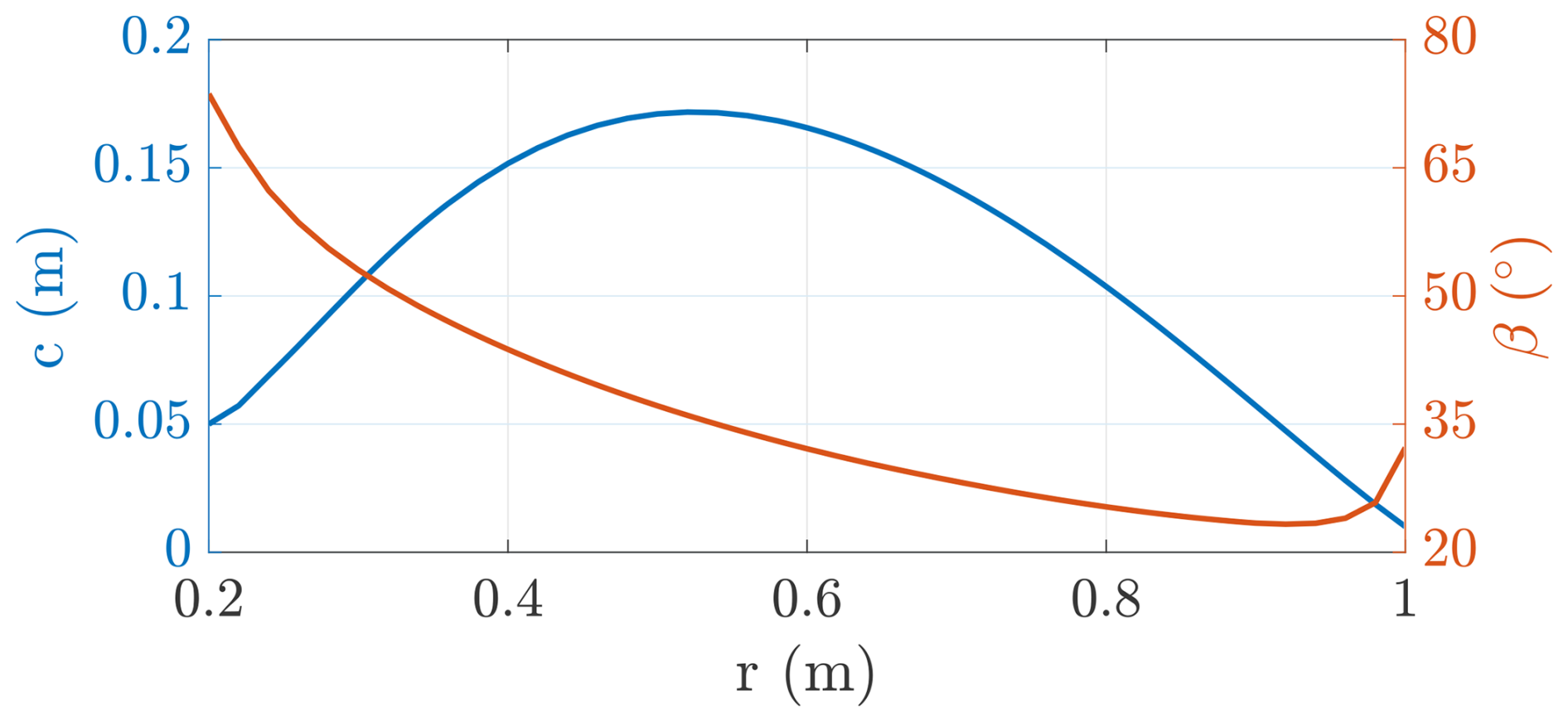
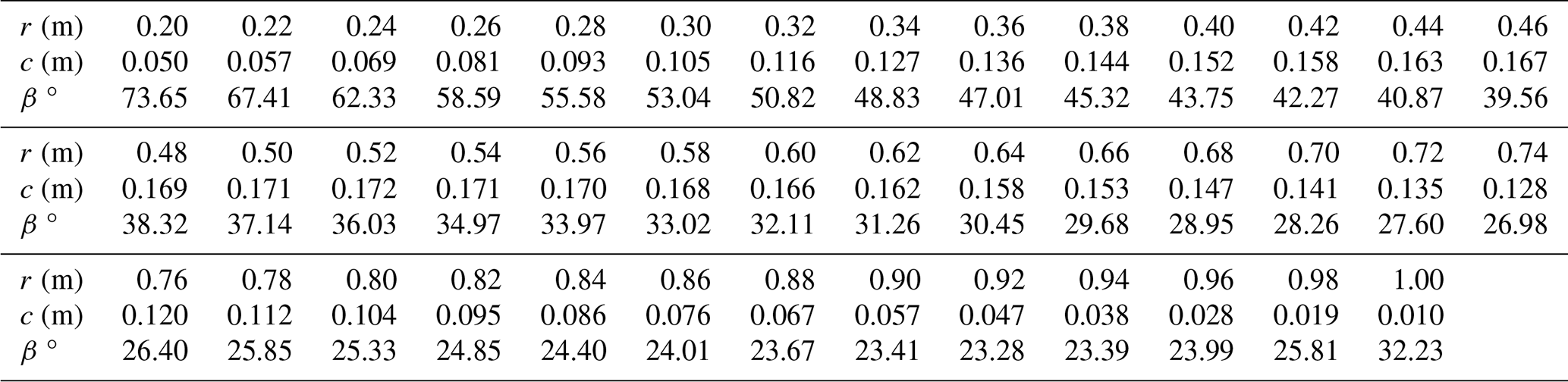
The onboard wind turbines' chord and twist are shown in Fig. 21. The values are given in Table C1. The twist changes drastically from the inner to the outer sections because the operational tip speed ratio λ_t is very low compared to conventional turbines. Recall that the chord and twist are slightly modified at the root and at the tip to achieve a realistic design with the methodology explained in Sect. 3. This leads to the increase in chord and twist at the root and at the tip.

Figure 21 Onboard turbine chord c and twist β as a function of the radius.

5.1 Isolated turbine

The onboard turbines are now studied with DUST, and the results are compared with the vortex cylinder model. The turbines' blades are modeled as lifting lines with 40 elements, and the simulation is run for eight revolutions with a time step corresponding to 5°, according to the convergence study performed in Appendix B. The turbines are simulated at a tip speed ratio of λ_t=1.91, finding a thrust coefficient of $C_{\mathrm{T},\mathrm{t}}=\mathrm{0.142}$, a power coefficient of $C_{\mathrm{P},\mathrm{t}}=\mathrm{0.122}$, and an efficiency of $C_{\mathrm{P},\mathrm{t}}/C_{\mathrm{T},\mathrm{t}}=\mathrm{0.86}$. These values are really close to the values found with the vortex cylinder model (Table 2, $C_{\mathrm{T},\mathrm{t}}=\mathrm{0.155}$, $C_{\mathrm{P},\mathrm{t}}=\mathrm{0.137}$, $C_{\mathrm{P},\mathrm{t}}/C_{\mathrm{T},\mathrm{t}}=\mathrm{0.88}$). The angle of attack and the corresponding sectional lift coefficients along the blade are shown in Fig. 22.

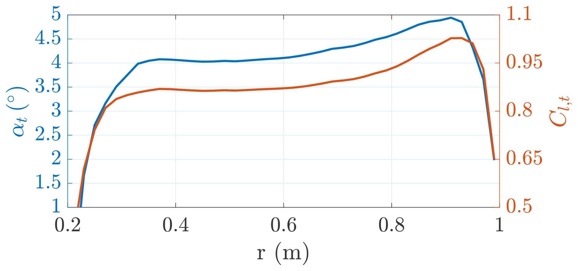
Figure 22 Onboard turbines' angle of attack α_t and lift coefficient C_l,t as a function of the radial coordinate (λ_t=1.91).

Figure 23 shows the induction of the turbines predicted by the vortex cylinder model and by DUST at a few distances from the rotor plane for λ_t=1.91. The trends show a good agreement at the rotor plane (0R_t), with DUST predicting slightly lower induced velocities. This could be due to the lower thrust coefficient. The trends after the rotor shows the change in air speed due to the wake expansion.

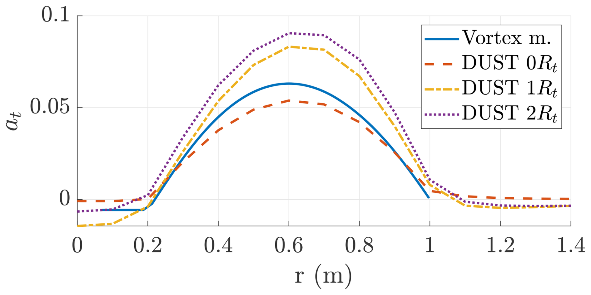
Figure 23 Onboard turbines' induction a_t as a function of the radial coordinate evaluated with the vortex cylinder model and with DUST at a few downstream distances (λ_t=1.91).

Figure 24 shows the change in inflow angle at different downstream positions. The vortex cylinder model and DUST are in good agreement at the rotor plane, with the vortex cylinder model predicting slightly higher change in inflow angle α_i,t.

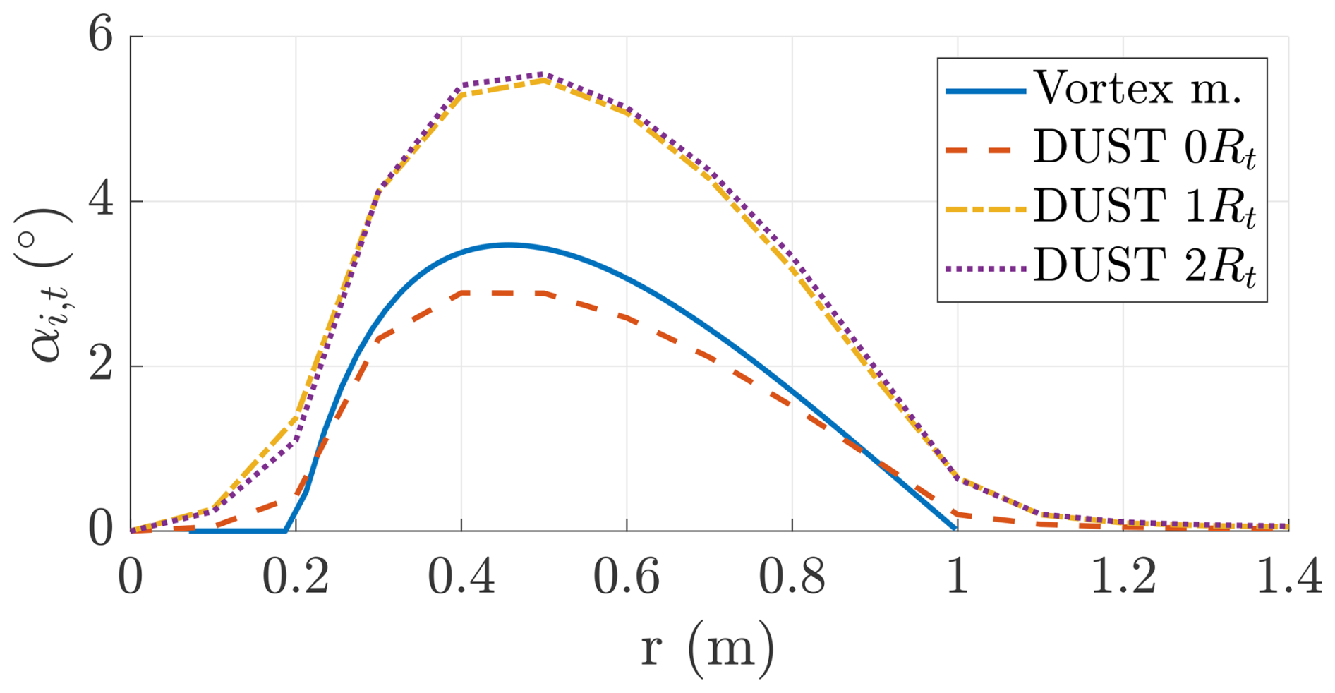
Figure 24 Onboard turbines' induced change in inflow angle α_i,t as a function of the radial coordinate evaluated with the vortex cylinder model and with DUST at a few downstream distances (λ_t=1.91).

To conclude the analysis of the turbine, the performance is studied for different tip speed ratios λ_t. Figure 25 shows the power and thrust coefficients of the turbines as a function of their tip speed ratio computed with DUST.

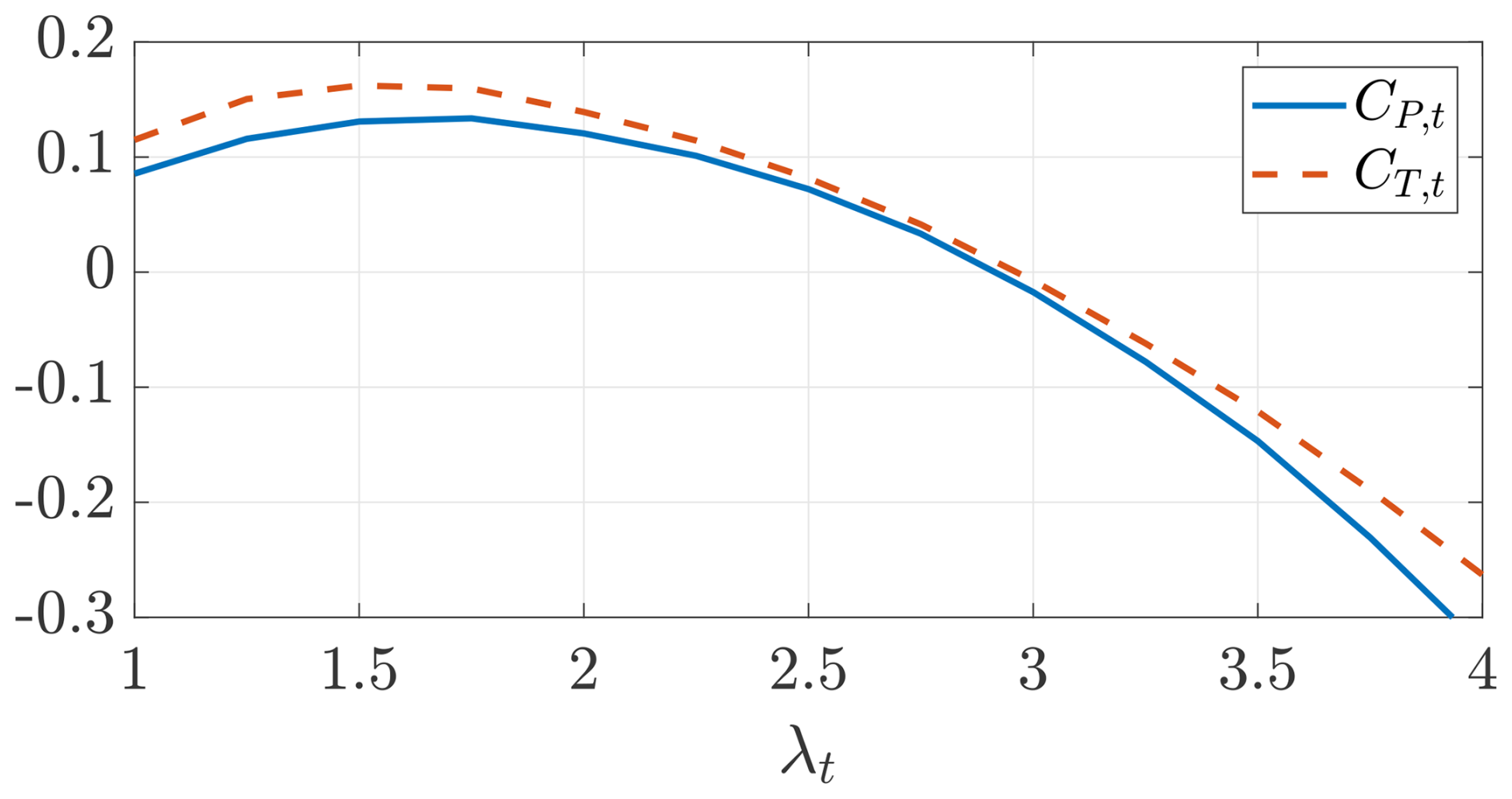
Figure 25 Onboard turbines' power coefficient C_P,t (−) and thrust coefficient C_T,t (− −) as a function of the tip speed ratio λ_t computed with DUST.

When the thrust coefficient reaches negative numbers, the turbine operates as a propeller. This turbine is designed to be fundamentally different from a conventional one for wind energy conversion. Indeed, its maximum power coefficient $C_{\mathrm{P},\mathrm{t}}\approx \mathrm{0.13}$ is far from the Betz limit as it is designed to maximize the windplane power coefficient C_P. The design tip speed ratio of λ_t=1.91 corresponds approximately to the maximum thrust and power coefficient. This means that these turbines cannot produce higher power and, thus, higher braking force, than their design value. Alborghetti et al. (2025) show how to control the windplane turbines in order to smooth the power output, highlighting the need to almost double the power coefficient with respect to the average value in some parts of the loop. Future works should then modify this design to cope with control requirements.

Figures 26 and 27 show the angle of attack and the lift coefficient along the blades for a tip speed ratio of λ_t=1.5 and λ_t=4, respectively. For low λ_t, the outer aerodynamic sections start experiencing positive stall, with the angle of attack exceeding 10°. For higher λ_t, the lift coefficients get to negative values, meaning that the thrust is generated in the opposite direction. The aerodynamic sections along the blade get closer to negative stall, which appears at $\mathit{\alpha }<-\mathrm{14}\mathit{°}$ (Re=200 000) or $\mathit{\alpha }<-\mathrm{16}\mathit{°}$ (Re=1 000 000) for the considered airfoil (NACA 4421).

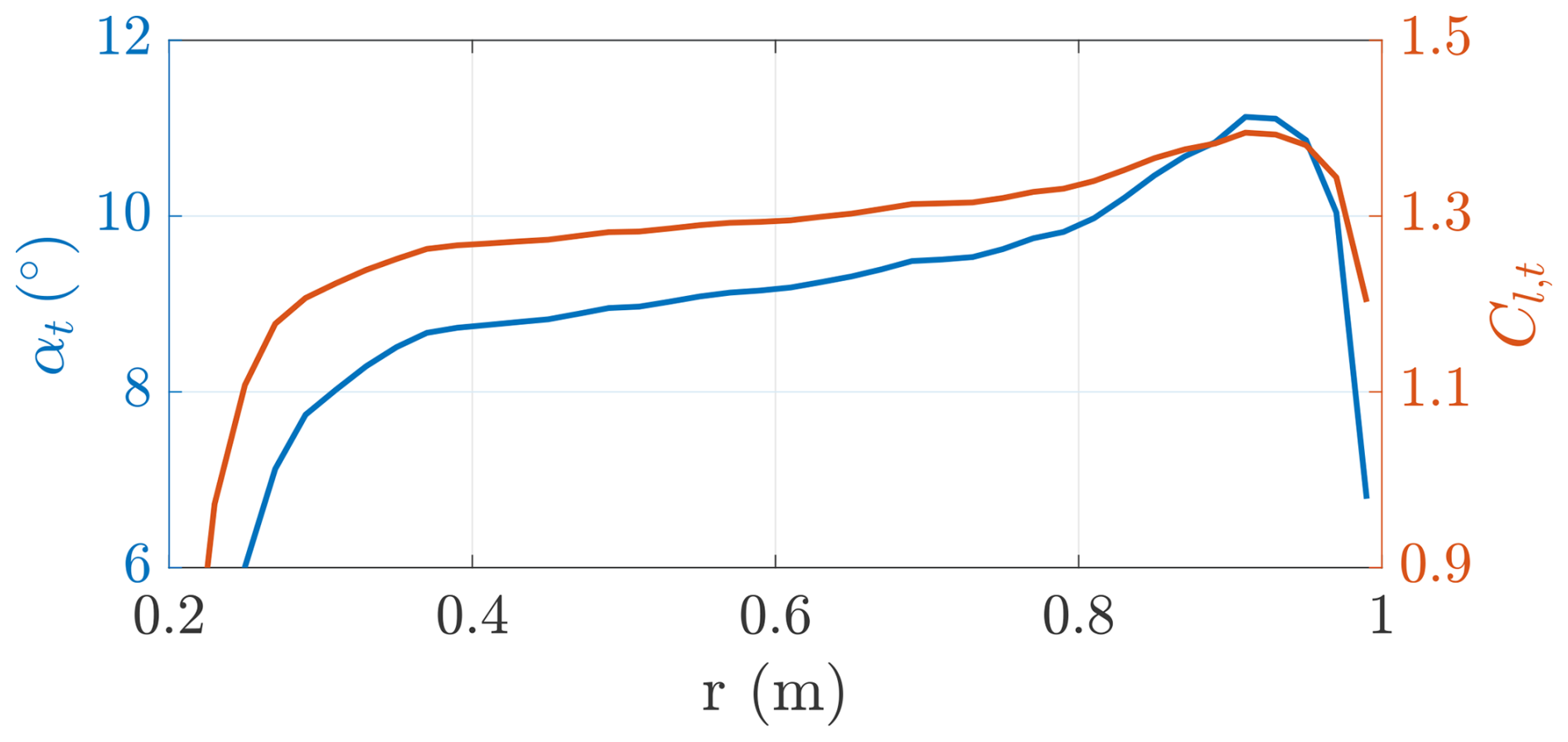
Figure 26 Onboard turbines' angle of attack α_t and lift coefficient C_l,t as a function of the radial coordinate (λ_t=1.5).

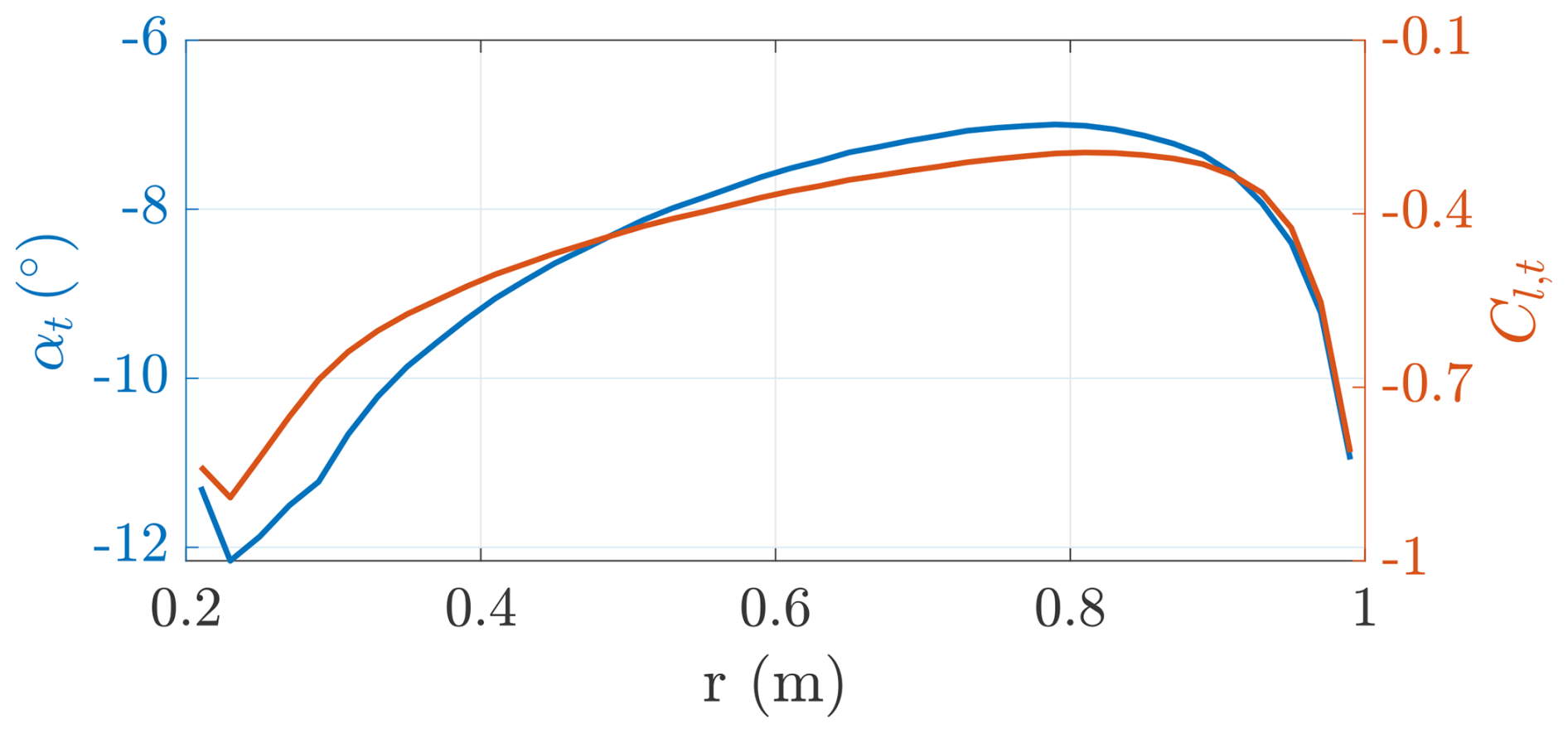
Figure 27 Onboard turbines' angle of attack α_t and lift coefficient C_l,t as a function of the radial coordinate (λ_t=4).

5.2 Isolated wing

The isolated wing is studied here with DUST and with the Weissinger lifting-line model developed for the design. We model the wing in DUST with vortex lattice elements. This modeling approach does not allow for an explicit evaluation of the wing sections' angle of attack and lift and drag coefficients, which can be recovered from the sectional loads. Moreover, this method only captures the induced drag and not the profile drag. The wing is discretized into 40 elements chord-wise and 60 elements span-wise in DUST, with a cosine distribution to better resolve the aerodynamics close to the wing tips, as shown in Fig. 20. The lifting line has the same span-wise discretization.

The lift and induced drag coefficients are presented in Figs. 28 and 29, showing a very good matching between the two approaches, while the lift and induced drag are shown in Figs. 30 and 31. The DUST simulation is run with a wing angle of attack of 11°, and the lifting line is run with a wing angle of attack of 12.2° to match the same wing lift coefficient of C_L=1.11. The wing-induced drag coefficient estimated with the two methods is $C_{\mathrm{D},\mathrm{i}}=\mathrm{0.074}$ (DUST) and $C_{\mathrm{D},\mathrm{i}}=\mathrm{0.072}$ (LL). The lift coefficient distribution (Fig. 28) informs us about the angle of attack distribution, which is influenced itself by the induced velocity distribution (recall that a constant twist is considered). The induced velocities for the considered wing are not constant, but they increase towards the tip, leading to lower angles of attack and thus lower lift coefficients.

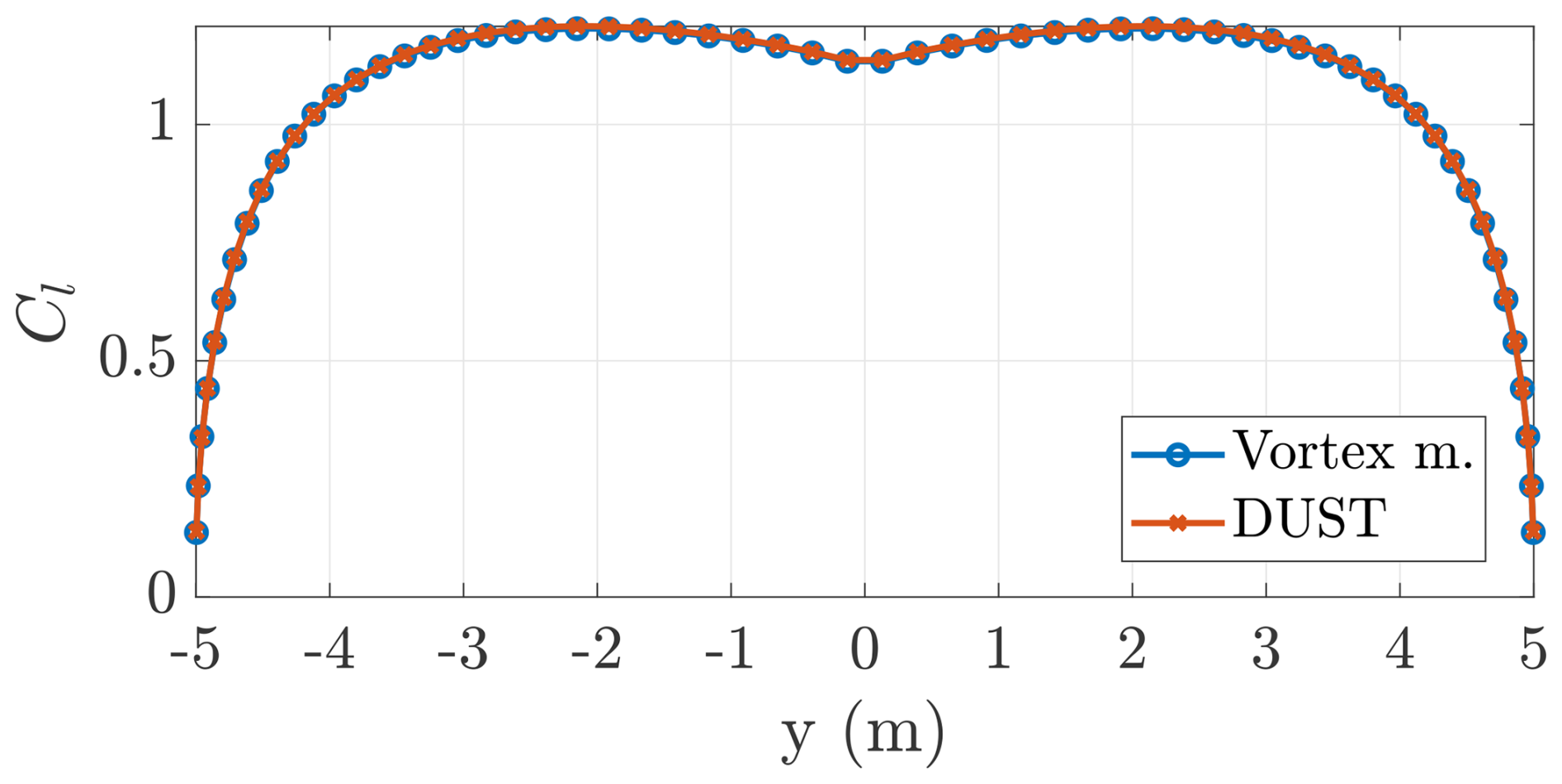
Figure 28 Distribution of lift coefficients along the wing span computed with the vortex model (lifting line) and with DUST.

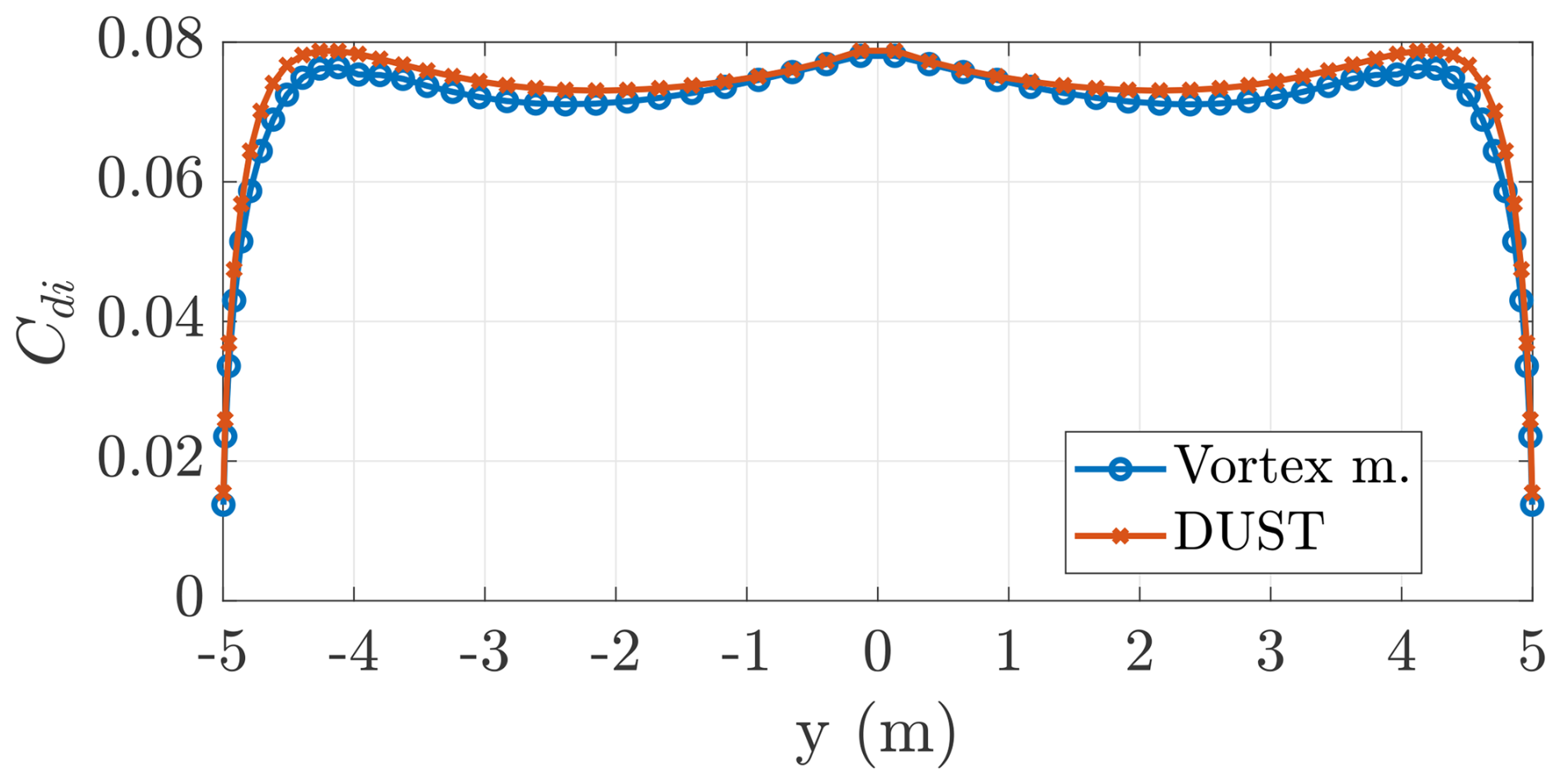
Figure 29 Distribution of induced drag coefficients along the wing span computed with the vortex model (lifting line) and with DUST.

5.3 Interactional aerodynamics

In this section, the interactional aerodynamics between the wind turbines, rotating inboard down, and the wing are studied. The complete problem is analyzed with DUST and with the interactional vortex model proposed in this paper. Figures 30 and 31 show the loads perpendicular to the inflow (lifting forces) and parallel to the inflow (induced drag forces) as estimated with the two methods. The trends of DUST are averaged over the last rotor revolution. The isolated wing results are also shown for reference.

The DUST simulation is run with a wing angle of attack of 11° at v_a=50 m s⁻¹, and the tip turbines are mounted with a tilt angle of −11°, such that the inflow is perpendicular to the rotor disk. The simulation is run for eight rotor revolutions with a time step equivalent to a rotor angle of 5°.

The vortex model is run with a wing angle of attack of 12.5° at v_a=50 m s⁻¹ to match the same integral lifting force computed with DUST of L=32.86 kN. The lift distribution of the solution with and without the turbines is almost identical. This is because of the 2-fold effect that the turbines produce on the following wing sections: they reduce the dynamic pressure by slowing down the apparent wind speed, thus reducing lift, and they modify the inflow angle such that the angles of attack increase, thus increasing lift. These two conflicting effects balance out to give a similar lift distribution. The wing-induced drag computed with DUST is D_i=2121 N, while, with the vortex model, it is D_i=2072 N. The wing spanwise efficiency computed with DUST (Eq. 54) is e_b=1.058, similar to the value computed with the vortex model e_b=1.080. The wind turbines in DUST have a thrust coefficient of $C_{\mathrm{T},\mathrm{t}}=\mathrm{0.148}$ and a power coefficient of $C_{\mathrm{P},\mathrm{t}}=\mathrm{0.129}$ , while, in the vortex model, they have the values shown in Table 2 ($C_{\mathrm{T},\mathrm{t}}=\mathrm{0.155}$,$C_{\mathrm{P},\mathrm{t}}=\mathrm{0.137}$).

The very good match between the vortex model and the DUST simulations proves that the vortex model developed in Sect. 2 captures the main physics of the interactional aerodynamics and thus is suitable for design and analysis.

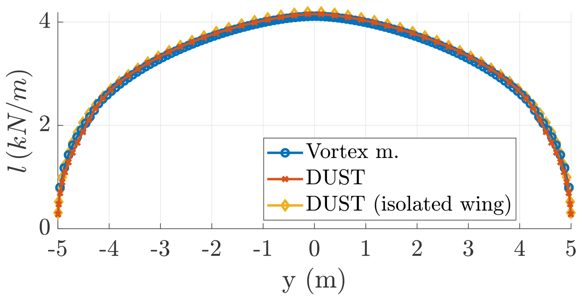
Figure 30 Aerodynamic loads acting on the wing perpendicular to the inflow – lifting forces – estimated with the vortex model and with DUST.

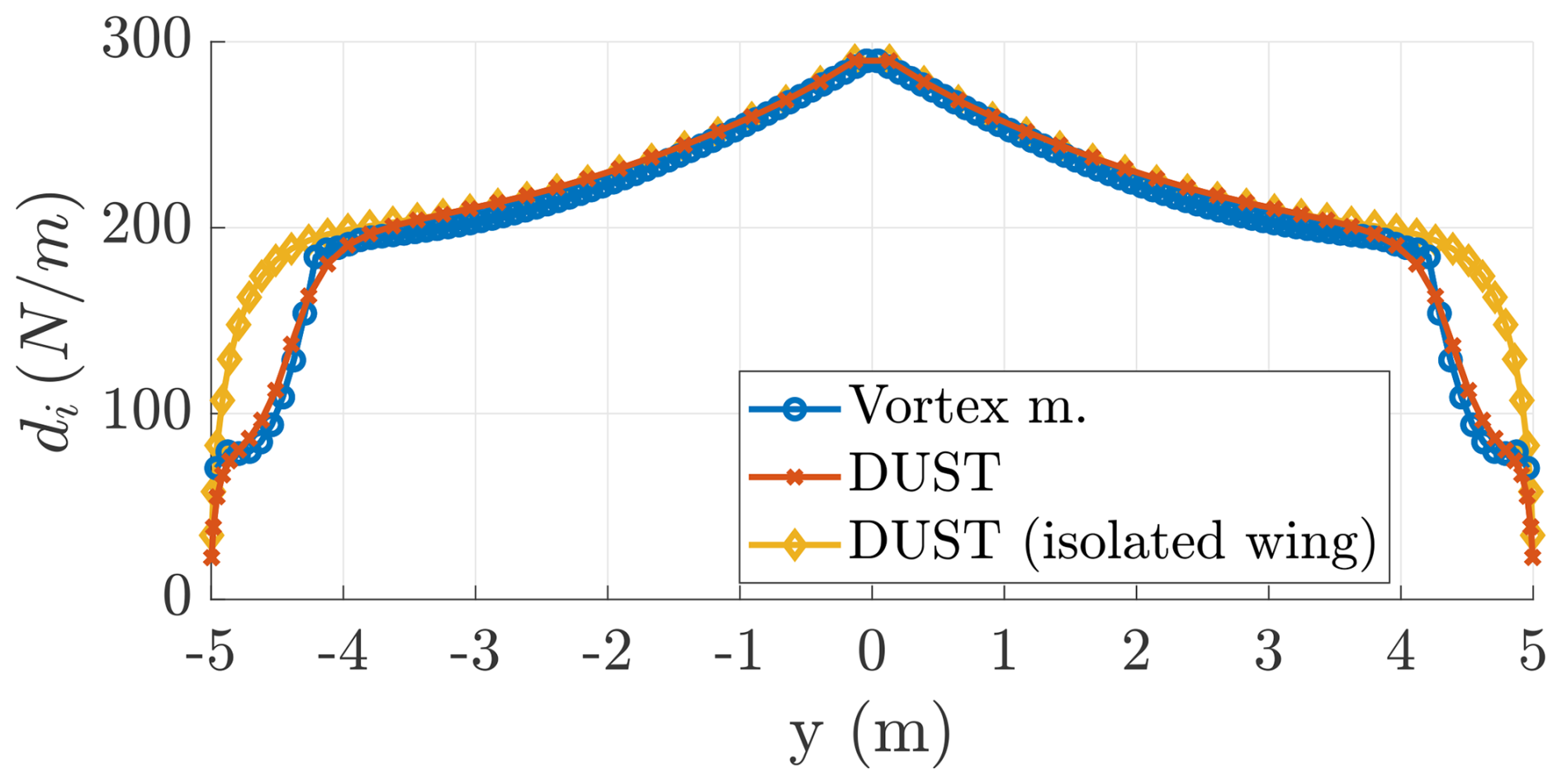
Figure 31 Aerodynamic loads acting on the wing parallel to the inflow – induced drag forces – estimated with the vortex model and with DUST.

5.4 Off-design analysis

To conclude, we analyze the windplane away from the design point. In this study, the isolated wing aerodynamics are exclusively influenced by the wing angle of attack α, while the isolated turbine aerodynamics are exclusively influenced by the onboard turbines' tip speed ratio λ_t. Figure 32 shows the windplane power coefficient C_P (Eq. 15) as a function of α and λ_t and is produced with the isolated wing polars (computed with DUST) and the isolated turbines' $C_{\mathrm{P},\mathrm{t}},C_{\mathrm{T},\mathrm{t}}$ curves (computed with DUST), thus neglecting the aerodynamic interaction between the turbines and wing. The far-wake induction is computed by estimating the tip vortices' strength Γ₀ (Eq. 45) and their position y_v (Eq. 46) from the local lift distribution in DUST.

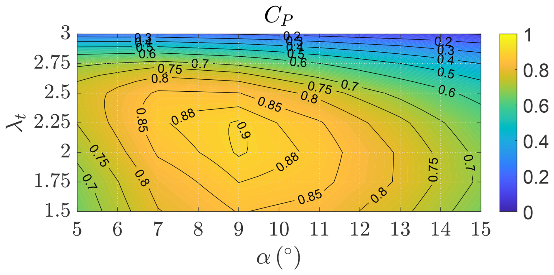
Figure 32 Power coefficient C_P as a function of the wing angle of attack α and the turbines' tip speed ratio λ_t, neglecting the aerodynamic interaction between the turbines and wing.

To include the interactional aerodynamics, we run DUST simulations for different combinations of α and λ_t, and we evaluate the windplane performances. Figure 33 shows the windplane power coefficient C_P (Eq. 15). The interactional aerodynamics are responsible for an increase in power production from C_P=0.90 to C_P=0.94. The power coefficient has an unconstrained maximum at α=9° and λ_t=2, which are far from the stall regions of the wing and of the turbine blades. While the power coefficient C_P informs us about the power production of the windplane, the thrust coefficient C_T, as in Fig. 34 (Eq. 16), informs us about the aerodynamic force generated by the windplane. To conclude the analyses of the design, Fig. 35 shows the wing speed ratio, informing us about the windplane speed u, as a function of α and λ_t. Clearly, the turbines have the strongest influence on the wing speed ratio as they act as a brake. It can be also noted that, for a given λ_t, λ has a maximum.

These three figures (Figs. 33 to 35) can be used to plan the high-level control of the windplane. Indeed, the windplane should be operated at the maximum power coefficient to maximize power production before the rated wind speed. To reduce the aerodynamic power after the rated wind speed, one could decrease the power coefficient by modifying the angle of attack α and the turbines' tip speed ratio λ_t. The control system might be developed to look for the combination of α and λ_t which minimizes the loads while keeping the desired C_P. By inspecting Fig. 34, the more sensible strategy to reduce the C_T is to reduce the angle of attack α. Increasing the tip speed ratio λ_t does decrease power but also increases the wing speed ratio λ (Fig. 35) and thus loads (Fig. 34).

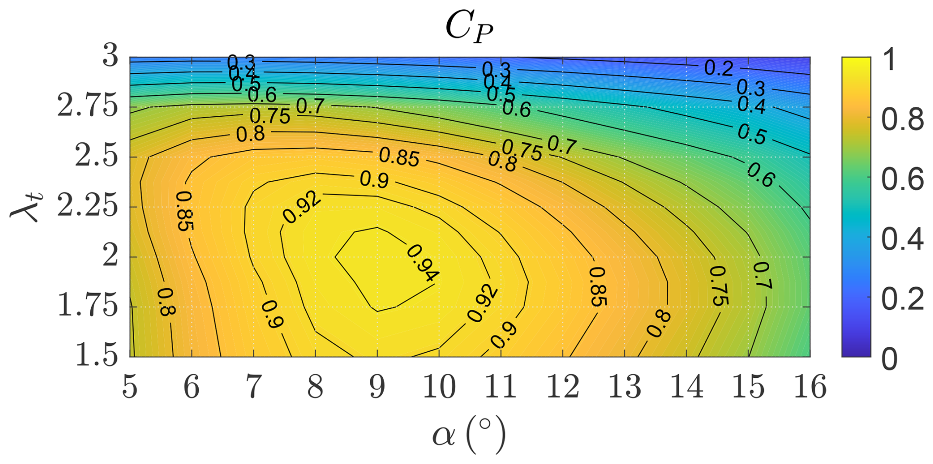
Figure 33 Power coefficient C_P as a function of the wing angle of attack α and the turbine tip speed ratio λ_t evaluated with DUST.

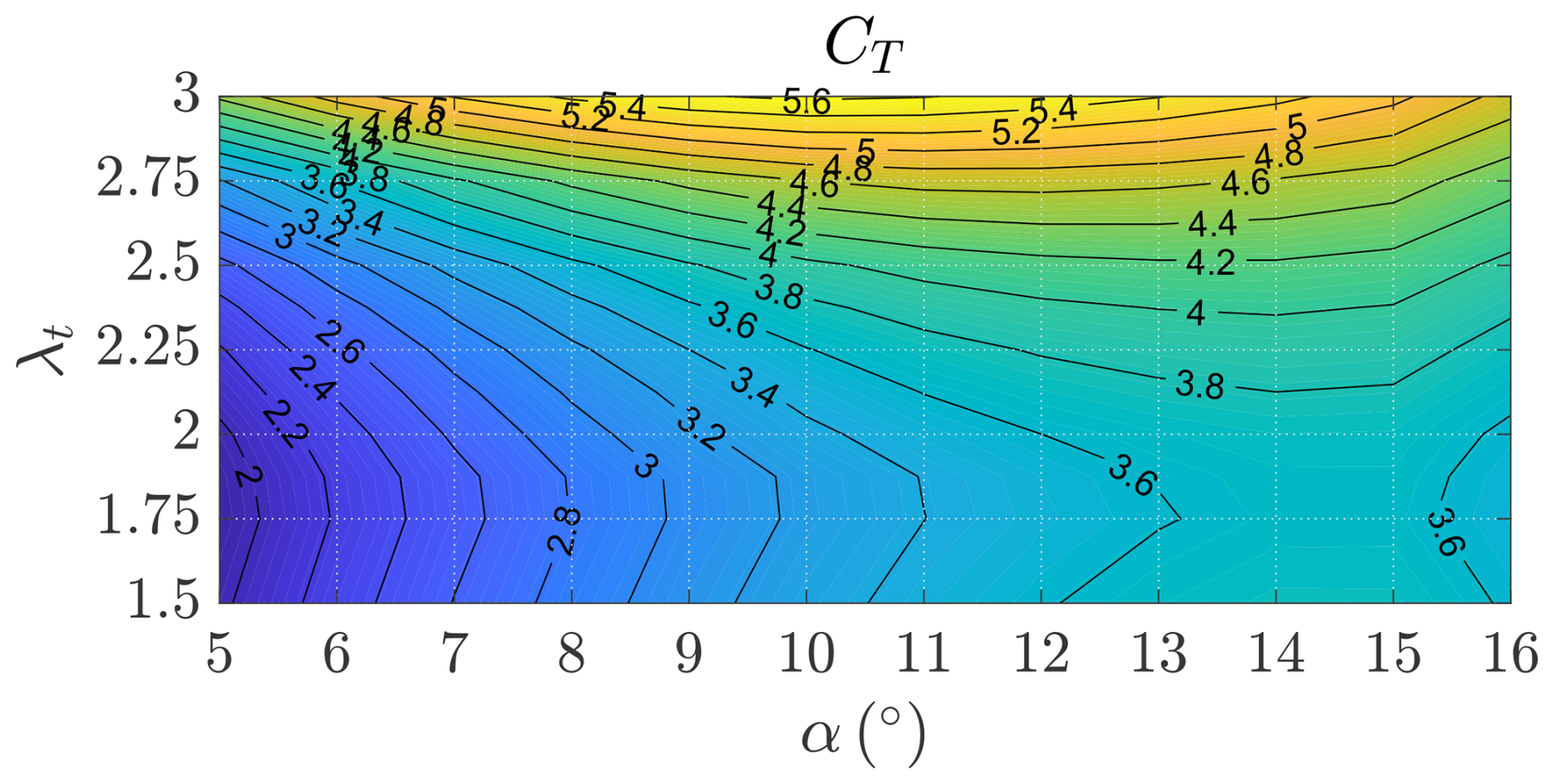
Figure 34 Thrust coefficient C_T as a function of the wing angle of attack α and the turbine tip speed ratio λ_t evaluated with DUST.

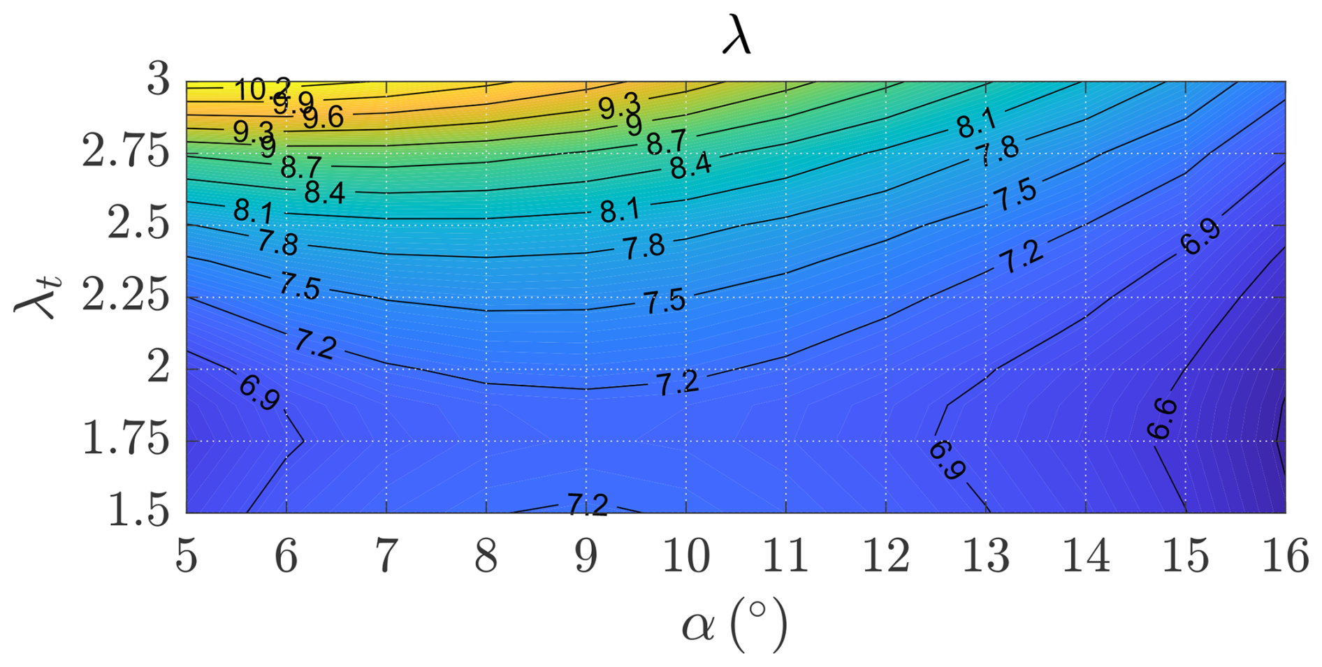
Figure 35 Wing speed ratio λ as a function of the wing angle of attack α and the turbine tip speed ratio λ_t evaluated with DUST.

Finally, Fig. 36 shows the induced drag as a function of the onboard turbines' tip speed ratio for α=10°. For low λ_t, the turbines swirl contributes largely to the reduction in the induced drag.

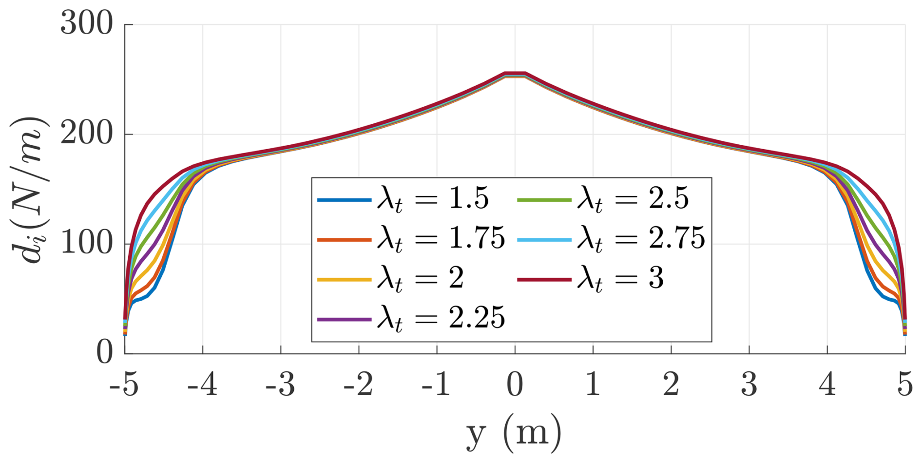
Figure 36 Spanwise distribution of induced drag d_i for different onboard turbine tip speed ratios λ_t.

6 Conclusions

In this paper, we develop a new methodology for the aerodynamic design and analysis of windplanes (the aircraft of fly-gen airborne wind energy systems), and we verify the methodology by comparison with higher-fidelity models and characterize the windplane design further with the vortex particle method.

In the method, a novel engineering model for the onboard turbines' aerodynamics, the wing aerodynamics, and their interactional aerodynamics is employed and coupled to a windplane steady-state model and a windplane far-wake model. The turbines are modeled as vortex cylinders, while the wing is modeled with a lifting-line formulation that accounts for the turbines' induced velocities. An optimization problem is formulated to concurrently design the turbines and the wing, assuming a trapezoidal planform and constant twist. The optimization objective is the windplane power coefficient, which uses as the reference area a disk with a radius equal to the wingspan. This is equivalent to taking as the objective the power while keeping the wingspan fixed. Other metrics could also be used as objectives in this framework.

Using the proposed approach, a design space exploration study is carried out to investigate the influence of turbine position and airfoil characteristics on the optimal design. We find that placing the turbines at the wing tips and rotating them inboard down leads to higher power production compared to mounting them on pylons (i.e., no interactional aerodynamics) or placing them in front of the wing. The key interactional effect arises from the turbine wake swirl, which modifies the inflow angle on the downstream wing sections. By choosing the correct rotor direction, inboard down, and placing the turbines at the wing tips, the outer part of the wing experiences an increase in inflow angles and thus an increase in performance. To enhance this beneficial effect, the optimal designs feature a larger wing taper ratio and a lower turbine tip speed ratio compared to other configurations. The design space exploration study also reveals that conventional efficient airfoils (high $C_{\mathrm{l}}/C_{\mathrm{d}}$) should be used in the design of windplanes, confirming the results of Trevisi (2024), rather than airfoils optimized for the $C_{\mathrm{l}}^{\mathrm{3}}/C_{\mathrm{d}}^{\mathrm{2}}$ metric commonly used in the literature. The wing aspect ratio is then designed such that the power is maximized when the wing, with constant twist, operates at the lift coefficient correspondent to the airfoil maximum efficiency.

Later, NACA4421 airfoils are considered for the aerodynamic optimization of the wing and of the turbines, placed at the wing tips. The turbines are characterized by an optimal tip speed ratio of λ_t=1.91, which dictates their twist and chord distribution. The wing is designed with a low aspect ratio (AR=5.1) and to operate at the lift coefficient corresponding to the airfoil maximum efficiency. The vortex models of the isolated turbines and the isolated wing and their aerodynamic interaction show very good agreement with the solution of the lifting line, the vortex lattice method, and the vortex particle method implemented in open-source code DUST. The behavior of the turbines is also studied with DUST as a function of the tip speed ratio. Finally, the windplane is studied with DUST at different angles of attack α and at different turbine tip speed ratios λ_t, finding the maximum power coefficient C_P=0.94 at α=9° and λ_t=2. The optimal operating point is far from the stall regions of the wing and of the turbine blades.

This paper describes a new comprehensive theory of the windplane aerodynamics, allowing for an in-depth understanding of the main aerodynamic phenomena. This work will be used as a baseline for more detailed aerodynamic studies on the turbines, wing, and tail. It could also be used for computing the aerodynamic derivatives to be used in flight stability analyses, for the closed-loop control development, for the structural design, and for airborne wind farm studies.

Appendix A: Nomenclature

Latin symbols
A	Wing area
af	Induction due the far wake
ar	Normalized axial velocity of the far-
	wake vortex rings
AR	Wing aspect ratio
at	Induction of the onboard turbine
b	Wing span
CD	System drag coefficient
CD,i	Induced drag coefficient
Cd,i	Sectional induced drag coefficient
CD,a	Wing drag coefficient due to the airfoils
CD,te	Equivalent tether drag coefficient
Cd,te	Drag coefficient of the tether section
CL	Wing lift coefficient
CP	Windplane power coefficient
CP,t	Onboard wind turbine power coefficient
CT	Windplane thrust coefficient
CT,t	Onboard wind turbine thrust coefficient
Dte	Tether diameter
E	Windplane aerodynamic efficiency,
	including the tether and the turbine thrust
eb	Spanwise efficiency
Lte	Tether length
m	Windplane mass plus one-third of the
	tether mass
R0	Turning radius
Rt	Onboard turbine radius
Rt0	Onboard turbine hub radius
tr	Taper ratio
u	Windplane tangential velocity
va	Apparent wind speed in the near wake
vw	Wind speed
Greek symbols
α	Wing angle of attack, defined as the angle
	between the x direction and the
	apparent wind speed va
αi,t	Induced change in inflow angle
	at the wing due to the turbine swirl
γn	Inflow angle in the near wake
λ	$\frac{u}{v_{\mathrm{w}}}$: wing speed ratio
λt	$\frac{{\mathrm{\Omega }}_{\mathrm{t}}{R}_{\mathrm{t}}}{u}$: onboard turbine tip speed ratio
Φ	Opening angle of the cone swept by the
	tether during one loop
ρ	Air density
ξt	$R_{\mathrm{t}}/(b/\mathrm{2})$ normalized onboard
	turbines radius

Appendix B: Turbine convergence study

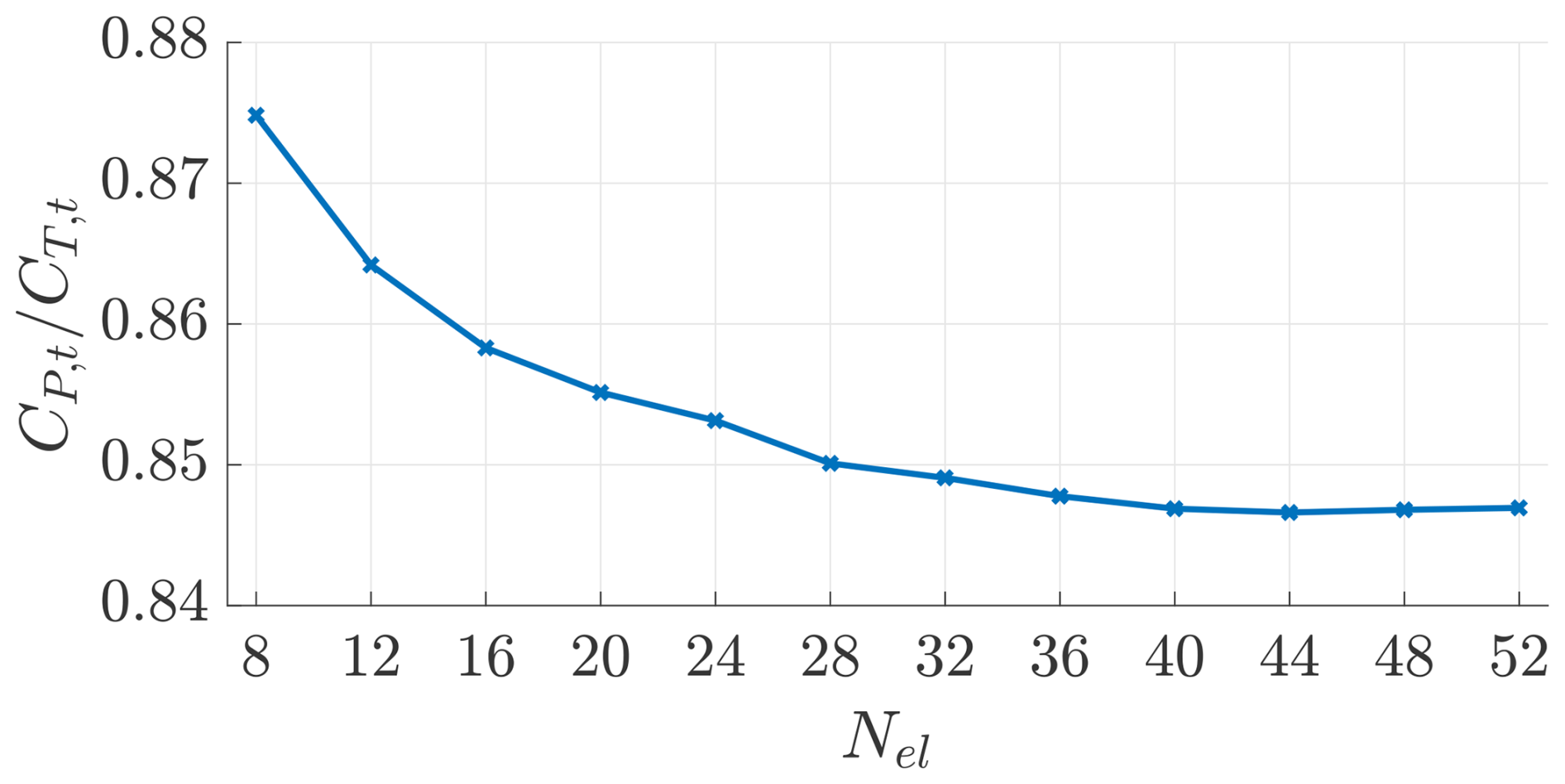
To select the number of lifting-line elements for the turbines for the simulations in DUST, we conduct a convergence study on an earlier turbine design, similar to the final design. For the turbines, we set a number of elements N_el and gradually increased them until the results converged, as shown in Figs. B1 and B2, leading to the use of 40 elements for the blade lifting line (Niro et al., 2024).

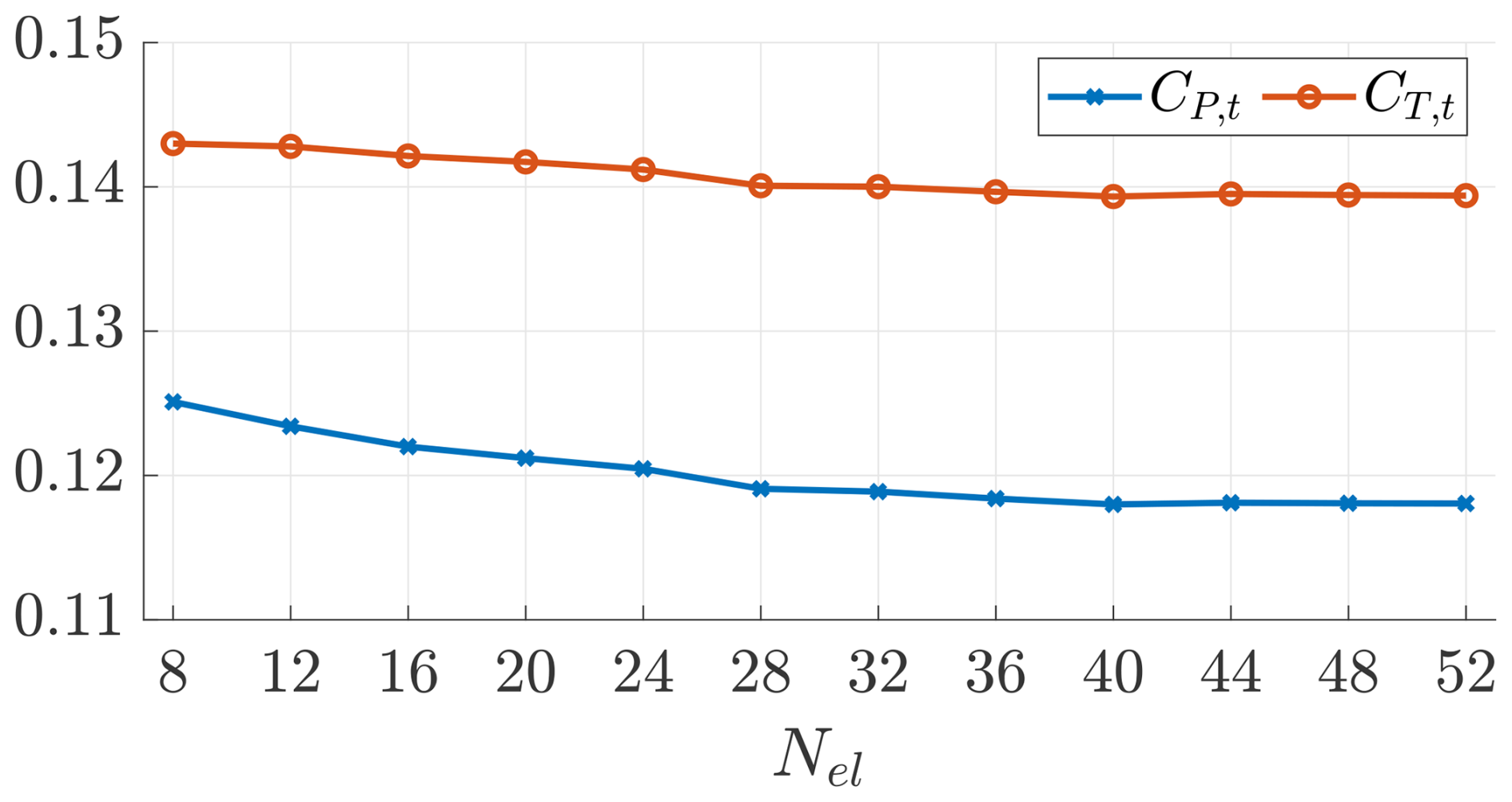
Figure B1 Power coefficient C_P,t and thrust coefficient C_T,t as a function of the lifting-line number of elements.

Figure B2 Turbine $C_{\mathrm{P},\mathrm{t}}/C_{\mathrm{T},\mathrm{t}}$ as a function of the lifting-line number of elements.

Figures B3 and B4 show the power and thrust coefficients and their ratio as a function of the number of rotor rotations. Even if a good convergence is experienced after approximately three rotations, the simulations in this paper are run for eight rotor revolutions. This second convergence study was carried out on the final turbine design.

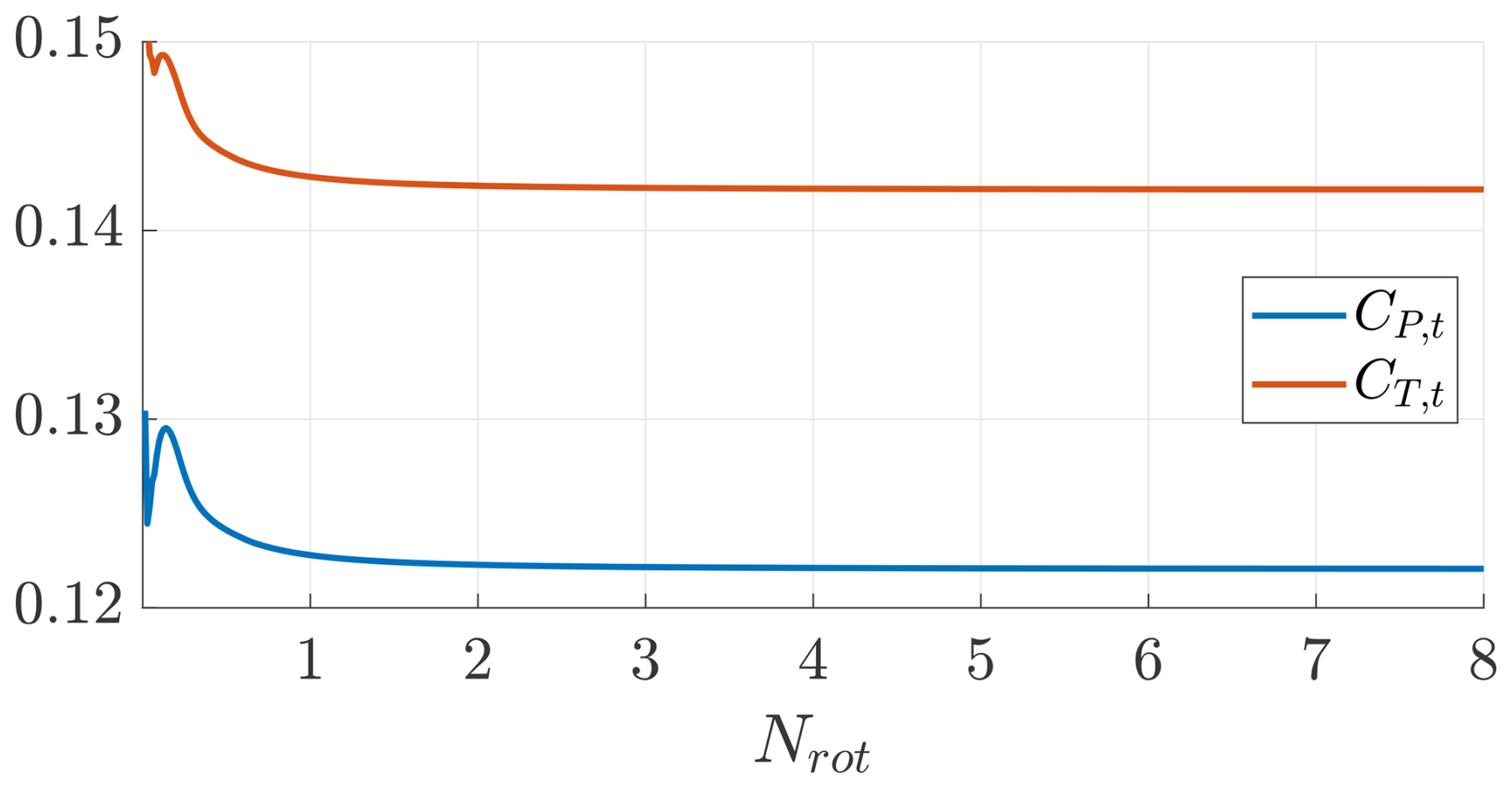
Figure B3 Power coefficient C_P,t and thrust coefficient C_T,t as a function of the rotor rotations (λ_t=1.91).

Figure B4 Turbine $C_{\mathrm{P},\mathrm{t}}/C_{\mathrm{T},\mathrm{t}}$ as a function of the rotor rotations (λ_t=1.91).

Appendix C: Turbine data

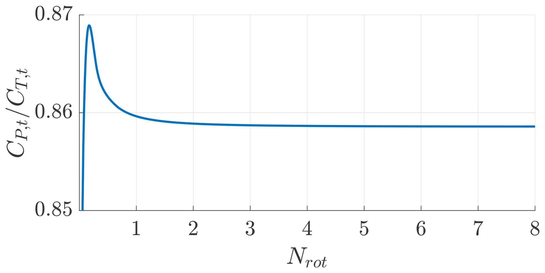
Table C1 Onboard turbine chord and twist distribution for R_t=1 m.