Performance of multi-band MDE-based virtual sensing for estimating lifetime fatigue damage equivalent loads for the IEA 15 MW reference wind turbine

Offshore wind turbines (OWTs) are increasingly susceptible to fatigue damage, motivating structure-wide stress monitoring for asset integrity management and life extension. Virtual sensing methodologies, such as multi-band modal decomposition and expansion (MDE), offer a solution to the above by extrapolating measurements from a few sensors at accessible locations to the global structure. However, most MDE studies model the rotor nacelle assembly (RNA) as a lumped-mass inertia, thereby ignoring rotor flexibility. This can lead to errors in estimated strains or stresses arising from erroneous mode shapes and the omission of relevant rotor modes from the estimates. The present paper quantifies these errors using HAWC2 simulations of the IEA 15 MW reference wind turbine (RWT). Multi-band MDE estimates of section moments are compared to true responses in terms of damage equivalent load (DEL) and stress (DES). Long-term estimates show that MDE accuracy depends on both the design load case and the elevation considered on the RWT support structure, with the MDE exhibiting notable errors near the tower top and at ±15 m around mean sea level (MSL). Furthermore, the error in the MDE estimates exhibits wind speed dependency, which underlines the inherent limitation of the MDE, assuming a linear and time-invariant response. In conclusion, multi-band MDE provides accurate estimates of section moments across most of the IEA 15 MW RWT support structure. However, improvements to the MDE may be achieved by the inclusion of rotor flexibility in the RNA model and environmental variability in the wave load Ritz vector.

1 Introduction

During recent decades, wind turbines have been consistently growing in size, and modern offshore wind turbines (OWTs) already on the market, such as the Vestas V236-15MW, now have a power production of up to 15 MW and rotor diameters approaching 240 m (Vestas Wind Systems A/S, 2026). At the same time, prototypes of the Mingyang MySE18.X-20 MW, with a power production of 20 MW and a rotor diameter of up to 292 m, and the Siemens Gamesa SG DD-276, with a power production of 21.5 MW and a rotor diameter of up to 276 m, have also been installed (Ghoshal, 2024; Salas, 2025). The growth in wind turbine size results in highly flexible support structures (tower, transition piece, and foundation), with the lowest natural frequencies approaching the quasi-static frequency domain. This makes them susceptible to dynamic excitation from turbulence and wave loads, resulting in designs that are increasingly vulnerable to fatigue damage (Zou et al., 2023). The same period has experienced the emergence of structural health monitoring (SHM), where data from sensors installed in a given structure are applied to inform operation and maintenance (O&M) strategies, asset integrity assessments, and lately also the assessment of potential life extension through monitoring of strain histories at fatigue-critical locations. However, for offshore structures, these critical locations are often sub-sea, where strain sensors are only accessible with significant effort, or sub-soil, where strain sensors cannot be installed or maintained in practice after erection. Furthermore, pre-installed sensors are likely to be damaged during erection, while any undamaged strain sensors tend to fail after a few years (Toftekær et al., 2023). To overcome these challenges, virtual sensing has gained traction in SHM of OWTs, where structural responses (stresses or strains) are estimated by so-called virtual sensors in which physical (above-sea) sensor signals are extrapolated to critical locations by a digital process model. Additionally, virtual sensing has the significant benefit of estimating the response of the structure at any location, hence not limiting the information from the structural health monitoring system (SHMS) to a few predefined sensor locations.

According to Zou et al. (2023), virtual sensing process models can be separated into two main categories. The deterministic approach uses model-based extrapolation, from which strain responses are estimated based on measurements from e.g. accelerometers, inclinometers, strain gauges, or 3D point tracking (Baqersad et al., 2015). The alternative probabilistic approach applies state estimation from Kalman filters (Maes et al., 2016); augmented Kalman filters (Vettori et al., 2023); dual Kalman filters (Eftekhar Azam et al., 2015); or, more recently, a generic latent force model (Bilbao et al., 2022; Zou et al., 2023). Lately, the use of neural networks has also entered the field of virtual sensing, e.g. when physics-guided learning from SCADA data and 10 min acceleration statistics are used to estimate damage equivalent moments (de N Santos et al., 2023) or when virtual sensors are trained based on strain sensors for gap filling in strain histories in case of sensor failure (Faria et al., 2025).

The present work applies the predominant deterministic model-based expansion method: modal decomposition and expansion (MDE). The concept of virtual sensing by MDE was initially introduced for dynamic strain estimation in OWTs in the pioneering work by Iliopoulos et al. (2014, 2016) and subsequently extended in Iliopoulos et al. (2017) to multi-band MDE, where strain histories are estimated individually in separate frequency bands (quasi-static, low frequency, and high frequency) based on measurements from strain gauges (for the quasi-static band) and accelerometers (for low- and high-frequency bands) using mode shapes and static deflection shapes from a finite-element (FE) beam model with lumped rotor nacelle assembly (RNA) inertia. This approach has been further developed by Noppe et al. (2016), using a SCADA-driven thrust load model for quasi-static band estimation, and by Henkel et al. (2021) for estimating and validating sub-soil fatigue stresses through dual-band MDE with experimental mode shapes and operational deflection shapes (ODSs).

The use of experimental ODSs and mode shapes is also applied for strain estimation using a synthetic response of the National Renewable Energy Laboratory (NREL) 5 MW reference wind turbine with an OC4 jacket substructure in Henkel et al. (2020), indicating less good performance for strains in the braces due to the occurrence of local brace modes and extrapolation of the wave loading. Augustyn et al. (2021) attempt to improve the estimation accuracy for jacket structures by including sensors in a few submerged braces and applying the wave-load-generated Ritz vectors from Skafte et al. (2017) and local brace modes in MDE.

Recently, Toftekær et al. (2023) have investigated the use of rotations obtained from filtered acceleration measurements in combination with Ritz vectors to estimate quasi-static stresses at the mud line of an 8.4 MW offshore wind turbine, thereby quantifying the accuracy of the estimated stress range histories for different modal expansion configurations. Subsequently, Fallais et al. (2024) have investigated the accuracy of a single-model MDE configuration for estimating damage equivalent stresses in the lower part of an OWT support structure, concluding that varying operational conditions across 2000 time series of 10 min duration only has a minor impact on the estimate precision.

Studies performing strain/stress estimates for monopile-supported OWTs, using MDE with mode shapes and Ritz vectors from an FE model (Iliopoulos et al., 2017; Noppe et al., 2016; Toftekær et al., 2023; Fallais et al., 2024), commonly consider the RNA to be lumped inertia. Consequently, the tower mode shapes that include blade motions are estimated inaccurately. This is demonstrated by Reinhardt et al. (2024), who show that ignoring blade flexibility in the RNA model significantly impacts the natural frequency and mode shape of the second tower bending modes. Additionally, rotor modes, which, given the inherent coupling between the tower and the blades, also affect the tower vibrations, are omitted from the MDE, as these cannot be represented using a lumped-inertia RNA model. These simplifications can therefore introduce errors in the strains or stresses estimated in the support structure. Furthermore, in the reviewed studies, the MDE performance is typically evaluated in the lower part of the support structure, where the influence from errors in the RNA model is less pronounced, thus giving an erroneous impression of their importance for the global response of the considered structure. Finally, these studies do not include wave loading separately in the MDE, thus assuming that wave loads are either insignificant or that the associated dynamic mode shapes can effectively capture their effects. However, these simplifications will lead to errors in the estimated strains and stresses in areas of the OWT support structure exposed to substantial wave loading.

The present paper addresses the errors associated with representing the rotor by lumped RNA inertia and its influence on the MDE prediction of damage equivalent loads (DELs) and stresses (DESs) in modern-scale offshore wind turbines. Furthermore, it investigates how wave loads can be explicitly included in the Ritz vectors for quasi-static and low-frequency estimation. For that precise purpose, uncertainties from soil modelling, variations in the OWT's as-built conditions, and measurement noise from sensors have been eliminated by considering the synthetic response data in Pedersen et al. (2025), which are an open-access dataset (available for download at https://doi.org/10.11583/DTU.24460090, Pedersen et al., 2025), containing response simulations covering the fatigue limit state (FLS) design life of the IEA Wind 15 MW offshore reference wind turbine with a monopile foundation (IEA 15 MW RWT) version 1.1.6 (Gaertner et al., 2020a).

The novel contributions of this paper are summarised as follows. The paper demonstrates the structure-wide performance of multi-band MDE by quantifying the error in terms of DES and DEL along the IEA 15 MW RWT support structure while applying a state-of-the-art lumped-inertia model for deriving mode shapes used in the MDE. It specifically shows how errors are associated with the second and third tower bending modes and the omission of rotor modes coupled to tower excitation. Additionally, this paper proposes a simple time-invariant load distribution for the wave load Ritz vector, which, to the best of the authors' knowledge, has not been explicitly defined in existing studies dealing with virtual sensing in OWTs on monopile foundations. Finally, this is the first work to utilise the Pedersen et al. (2025) dataset. This dataset facilitates cross-institute benchmarking of virtual sensing algorithms, as it provides an unrestricted range of sensor locations and associated output channels. Furthermore, it enables validation of the predicted response in the entire OWT, including the monopile, tower, and blades.

The structure of the paper is as follows. Section 2 briefly presents the data from Pedersen et al. (2025), and Sect. 3 presents the assessment of the performance of the IEA 15 MW RWT, along with a relative lifetime damage calculation made for the individual design load cases included in Pedersen et al. (2025). Section 4 explains the multi-band MDE methodology used in the present work and the finite-element (FE) model used to extract mode shapes and Ritz vectors for the MDE. In Sect. 5, the MDE is used for the estimation of damage equivalent loads (DELs) and stresses (DESs), and the MDE errors are quantified and discussed, with Sect. 6 providing conclusions and perspective for future work.

2 Data

The present work is based on synthetic wind turbine response data from the online open-access dataset IEA-15MW-RWT-Monopile HAWC2 Response Database (Pedersen et al., 2025), which is available for download at https://doi.org/10.11583/DTU.24460090 (Pedersen et al., 2025) along with the relevant documentation, model and input files, and scripts for reading and sorting data. The dataset comprises 4902 HAWC2 output files covering the fatigue limit state (FLS) design life of the IEA 15 MW RWT (presented in Fig. 1) version 1.1.6, which is described in Gaertner et al. (2020a).

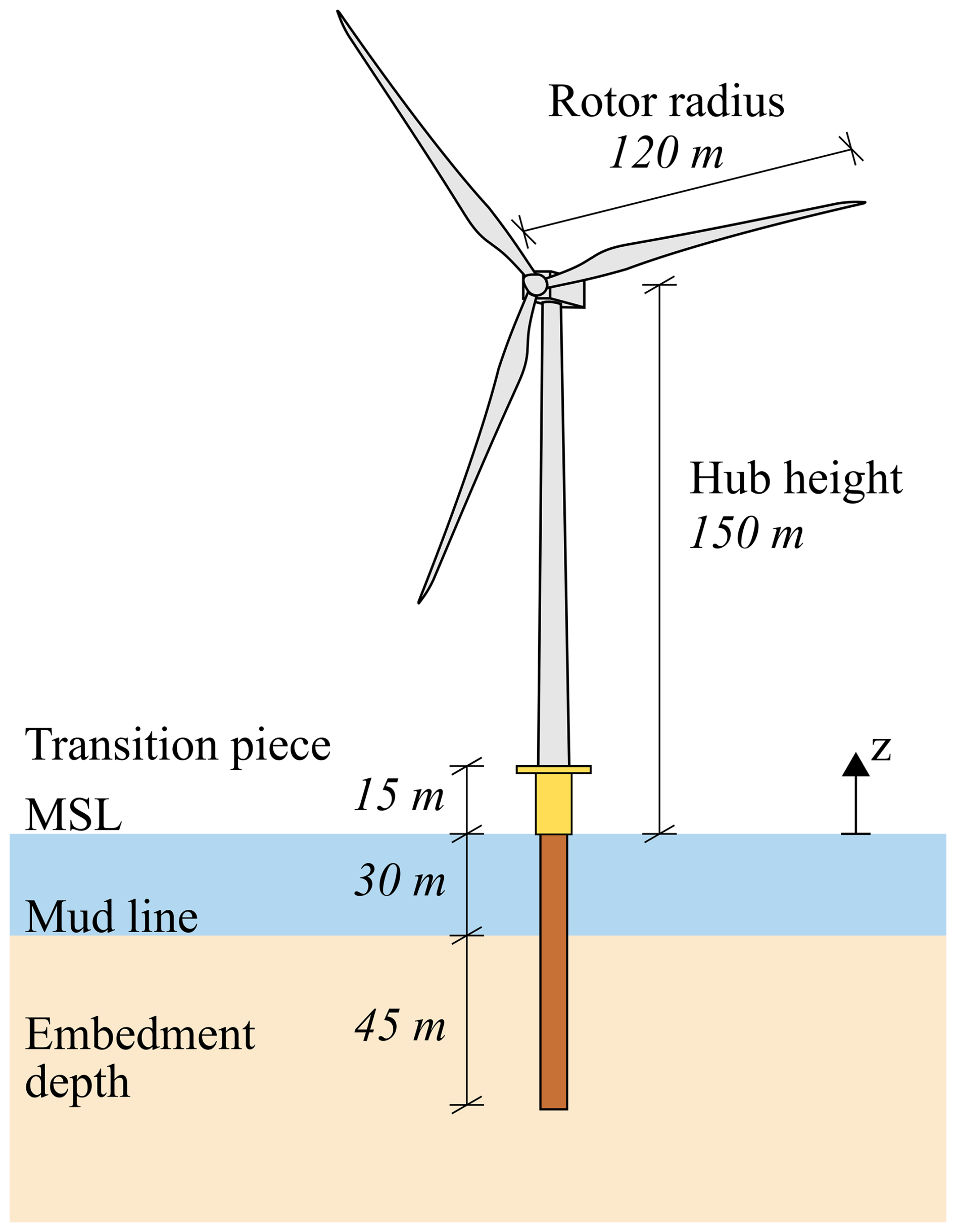
Figure 1 Overview of the IEA 15 MW RWT (data from Gaertner et al., 2020a). The RWT has a hub height of 150 m above mean sea level (MSL) and a rotor radius of 120 m. The water depth at the chosen site is 30 m. The support structure of the RWT consists of a 75 m monopile with an embedment depth of 45 m, a 15 m transition piece, and a 129.4 m tower.

The metocean data used for the simulations performed by Pedersen et al. (2025) are based on the metocean assessment performed for Energinet Eltransmission A/S in DHI (2023a), DHI (2023b), and DHI (2023c). The individual HAWC2 output files contain time series data from 898 sensors, hereunder environmental and operational data (e.g. hub wind speed, wave height, rotor speed, blade pitch angles, torque, thrust, and power production) and structural response data in terms of displacements, rotations, accelerations, forces, and moments in the individual structural members.

Appendix A briefly describes the IEA 15 MW RWT and the modelling assumptions and design load cases (DLCs) considered in Pedersen et al. (2025).

3 IEA 15 MW RWT performance and relative damage assessment

In the present section, the performance of the IEA 15 MW RWT is assessed based on the data presented in Sect. 2. Subsequently, the relative lifetime damage from the individual DLCs from Pedersen et al. (2025) is calculated for the IEA 15 MW RWT, based on DELs.

3.1 Performance of the IEA 15 MW RWT

When performing modal decomposition and expansion (MDE), modal truncation is needed due to a limited number of sensors. Furthermore, a finite number of Ritz vectors can be included to assess the quasi-static part of the response. Hence, it is important to have an overview of the different governing loads to be accounted for in the response estimates. This section gives an example of how diverse operational and environmental conditions can impact the DELs of the IEA 15 MW RWT and hence contribute differently to lifetime damage. Specifically, statistical values of relevant operational parameters and the tower base fore–aft (FA) and side–side (SS) section moments are considered during normal power production (DLC 1.2).

In Fig. 2, the statistics (minimum, mean, maximum) of the operational parameters (rotor speed, electrical power, generator torque, thrust, and pitch angle) and the wave amplitude are presented, while Fig. 3 shows the associated statistics of the tower base FA and SS section moments and the 1 Hz DELs for the individual HAWC2 time series (evaluated by Eq. 4) for DLC 1.2. The operational parameters in Fig. 2 are compared with steady-wind rotor performance values from Gaertner et al. (2023), generated by the Wind-plant Integrated System Design and Engineering Model (WISDEM), which uses the aeroelastic code OpenFAST.

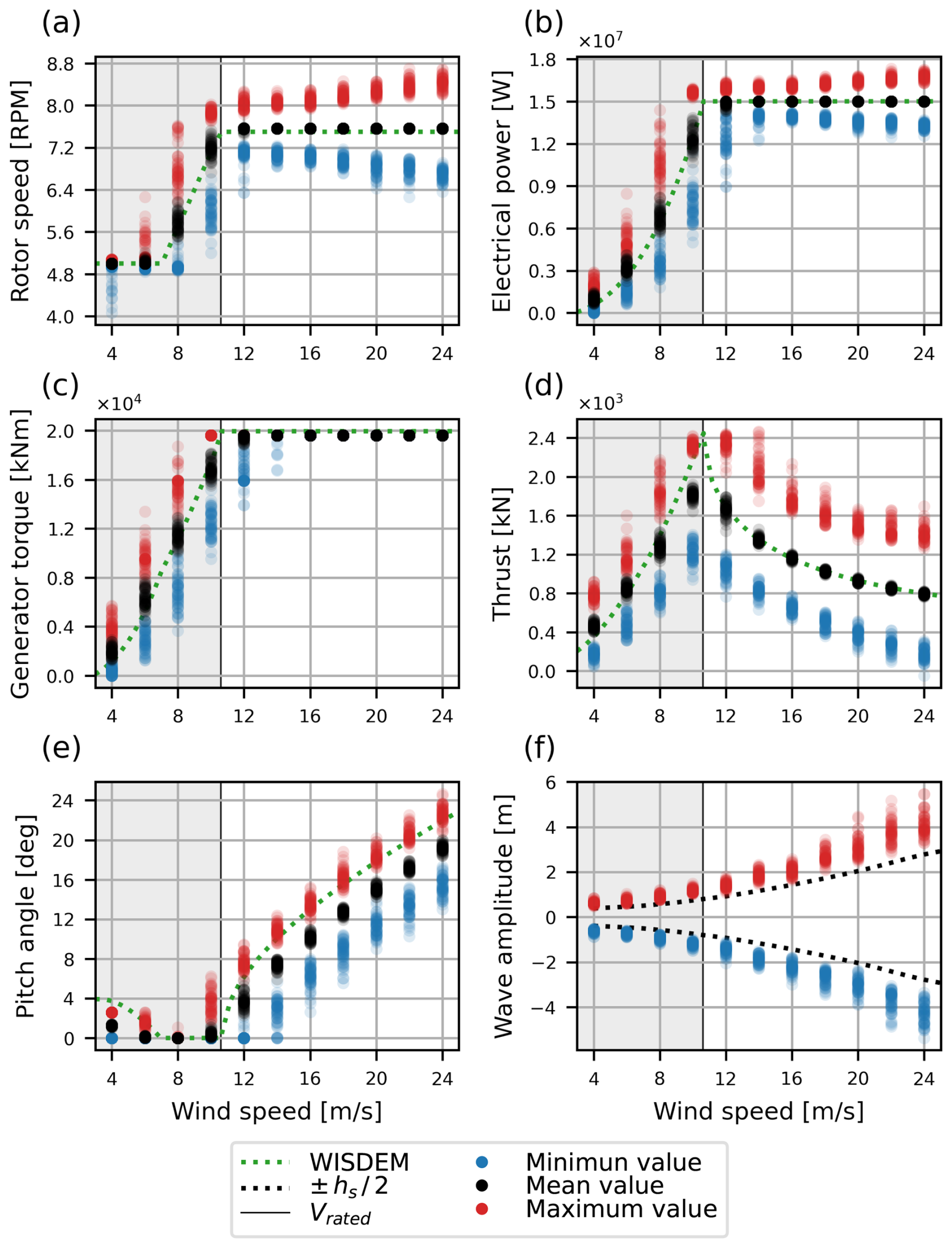
Figure 2 Statistical values (minimum, mean, maximum) for selected operational parameters: (a) rotor speed, (b) electrical power, (c) generator torque, (d) thrust load, (e) pitch angle, and (f) wave amplitude depicted across the wind speed at the hub, calculated for the HAWC2 time series covering DLC 1.2 for the mean water level (MWL) equal to MSL.

Figure 2a–e show that the mean values generally coincide well with the WISDEM output, and Fig. 2f verifies that the minimum and maximum wave amplitudes follow the development of the input significant wave height. The greatest discrepancies are observed for the thrust in Fig. 2d and the pitch angle in Fig. 2e. The discrepancies in the thrust and pitch angle are due to steady versus turbulent operation and the ElastoDyn beam model used in the WISDEM calculation (Gaertner et al., 2020b) not including a torsional degree of freedom (Rinker et al., 2020). The generally good match between the models indicates that the HAWC2 model may be used for further analysis.

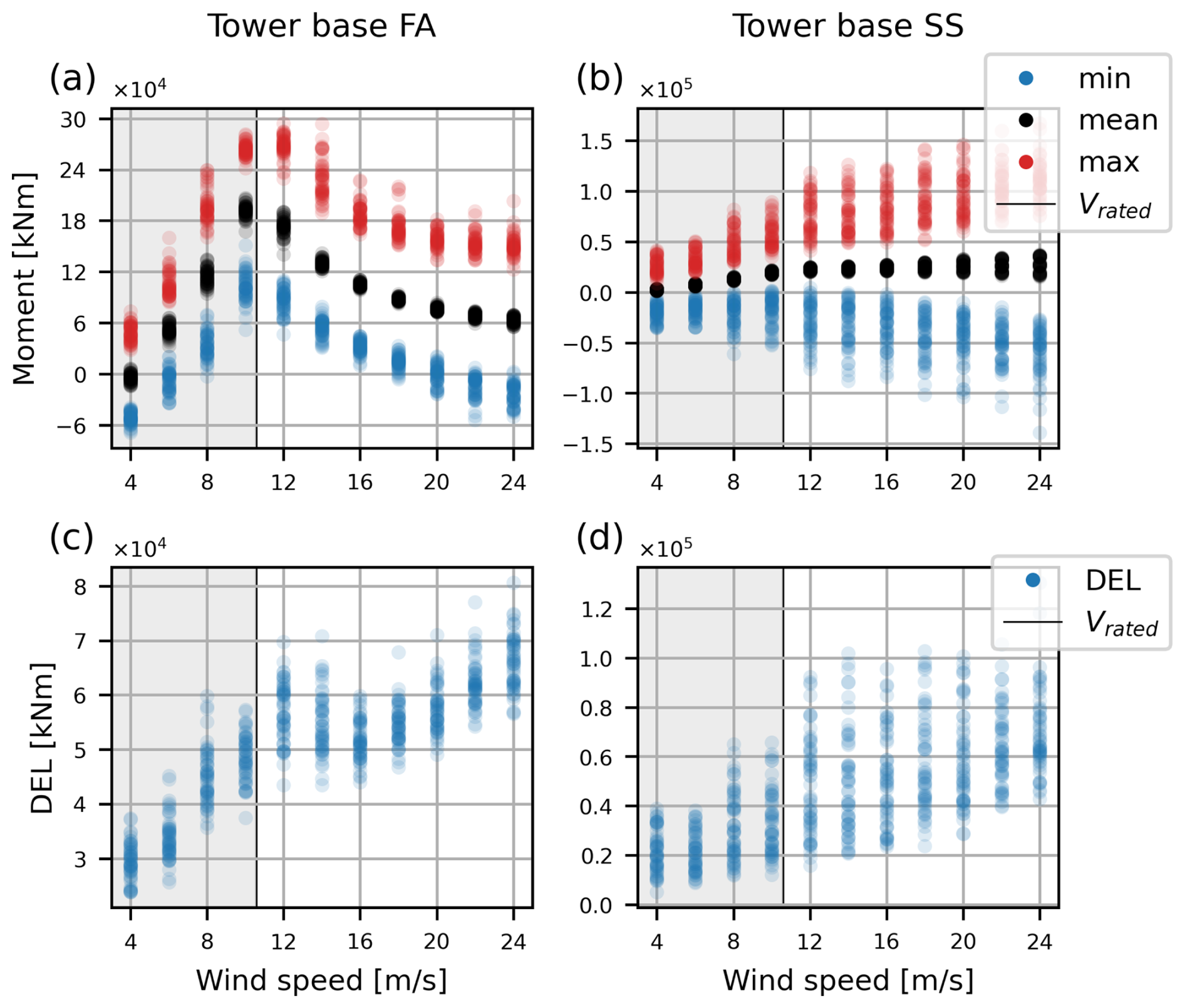
Figure 3 Statistical values (minimum, mean, maximum) of the tower base moment calculated in (a) the FA direction and (b) the SS direction and DELs calculated in (c) the FA direction and (d) the SS direction, all based on the HAWC2 time series covering DLC 1.2 for the MWL equal to MSL.

The statistical values for the tower base FA moment presented in Fig. 3a follow the thrust curve from Fig. 2d as expected. The DELs associated with the tower base FA moment presented in Fig. 3c generally increase with both the wind speed and turbulence. However, they plateau at wind speeds from approximately 12–16 m s⁻¹, in which range the blades start to pitch (see Fig. 2e). This illustrates that the DELs in the FA direction at the tower base are primarily governed by quasi-static wind loading, while operational parameters (e.g. the pitch angle) also affect the damage. Similarly to the statistical values of the tower base FA moment, the mean values of the tower base SS moment presented in Fig. 3b follow the generator torque curve in Fig. 2c. The minimum and maximum values of the tower base SS moment are symmetric around the mean value with increasing amplitudes for increasing wind speeds. The associated DELs in Fig. 3d also increase with the wind speed and turbulence. Furthermore, Fig. 3d shows that the variance in the DELs increases with the wind speed up to rated wind speed, from where it is rather significant.

To assess the cause of the high variance, the time histories of the tower base SS moment, wind speed (in the SS direction), and wave height associated with the minimum and maximum DELs for the wind speed of 14 m s⁻¹ are presented in Fig. 4. Considering the moment time series in Fig. 4a and the related PSD in Fig. 4b, it is concluded that DELs are mainly driven by the first tower SS mode. There is not a significant difference in the frequency content of the wind around the natural frequencies of the first-order tower bending modes. However, the mean wind speed in the SS direction is significantly higher for the maximum DEL than for the minimum DEL due to the −10° yaw error. Furthermore, the waves have an angle of attack of −32.5° for the maximum DEL, whereas it is 0° for the minimum DEL. Thus, the variation in DEL magnitude is caused by the excitation of the first tower SS mode occurring for the maximum DEL, while not for the minimum DEL, likely due to the difference in the excitation forces resulting from the varying angle of attack of the wind and waves between the two time series.

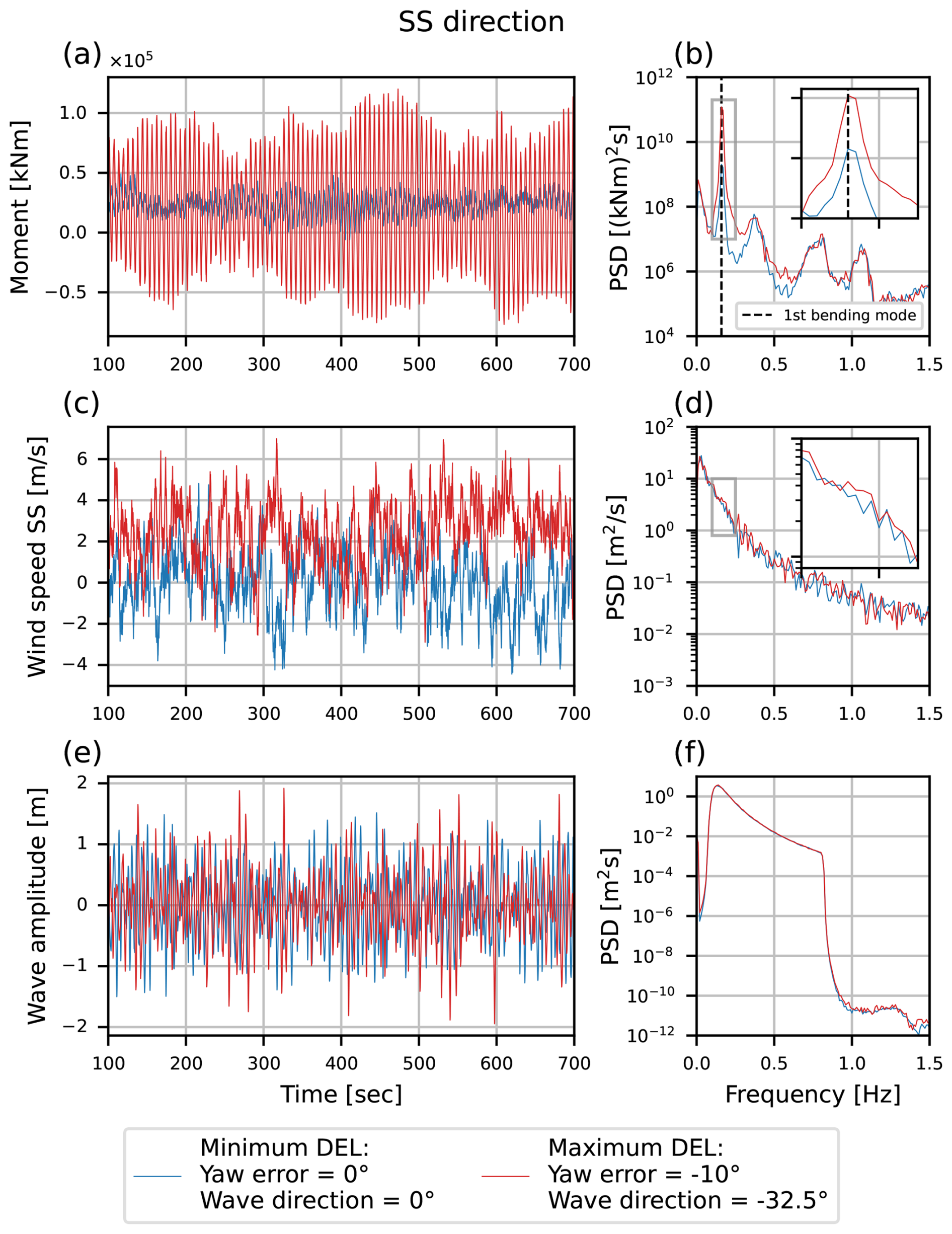
Figure 4 Time series data for maximum and minimum DELs from Fig. 3d at 14 m s⁻¹ hub wind speed: (a) time history and (b) PSD of tower base moment in the SS direction, (c) time history and (d) PSD of hub wind speed in the SS direction, and (e) time history and (f) PSD of wave amplitude (water surface elevation).

In conclusion, the present section underlines that the DELs calculated for the IEA 15 MW RWT are indeed influenced by environmental parameters such as turbulence, which govern the quasi-static response, and wave direction. Furthermore, operational parameters such as pitch angles and yaw errors can, in some cases, contribute to the excitation of the dynamic modes, which significantly impacts the DELs. Thus, the MDE configuration presented in Sect. 5.1 is required to accurately capture both quasi-static and dynamic responses for varying operational and environmental conditions.

3.2 Relative lifetime damage results

The present section investigates the lifetime damage of the IEA 15 MW RWT caused by the individual design load cases presented in Sect. A3, thereby giving an overview of which operating scenarios are significant for the fatigue damage in the support structure.

According to Veldkamp (2006), the relative lifetime damage caused in a given structure by a load case i is given as

$$\begin{array}{}\text{(1)}& d_{i,\mathrm{rel}}={\displaystyle \frac{n_i(\mathrm{\Delta }{P}_{\mathrm{eq},i}{)}^m}{n_{\mathrm{T}}(\mathrm{\Delta }{P}_{\mathrm{eq}}{)}^m}},\end{array}$$

where ΔP_eq,i represents the 1 Hz DEL ranges for the individual load case i, m is the Wöhler coefficient, n_i is the number of 1 Hz cycles for load case i, n_T is the total number of 1 Hz cycles in the structure's lifetime, and ΔP_eq is the lifetime DEL range.

In the present analysis, a similar approach to that of Veldkamp (2006) in Eq. (1) is used for the evaluation of the relative lifetime damage for individual DLCs. By adding the 1 Hz DELs from the HAWC2 simulations contained in a DLC, the relative damage of the individual DLCs is calculated as

$$\begin{array}{}\text{(2)}& d_{\mathrm{DLC},\mathrm{rel}}={\displaystyle \frac{{\sum }_{\mathrm{s}\in \text{DLC}}{n}_{\mathrm{s}}(\mathrm{\Delta }{P}_{\mathrm{eq},\mathrm{s}}{)}^m}{n_{\mathrm{T}}(\mathrm{\Delta }{P}_{\mathrm{eq}}{)}^m}},\end{array}$$

where

$$\begin{array}{}\text{(3)}& n_{\mathrm{s}}=p(\text{DLC},V,{\mathit{\theta }}_{\mathrm{yaw}},{\mathit{\theta }}_{\mathrm{wwm}}){\displaystyle \frac{n_{\mathrm{T}}}{n_{\mathrm{seed}}}}\end{array}$$

is the number of 1 Hz cycles during the lifetime of the IEA 15 MW RWT, p( ) is the joint probability of the input parameters for the operational and environmental conditions (DLC, wind speed (V), yaw error (θ_yaw), and wind–wave misalignment (θ_wwm)) used for the simulation s, and n_seed is the number of simulations that share these operational and environmental conditions. Note that the number of summations in Eq. (2) refers to the number of (converged) simulations in Table A2 for a given DLC at MWL equal to MSL. Finally, in Eq. (2) the 1 Hz DEL range for the individual HAWC2 simulations is evaluated as

$$\begin{array}{}\text{(4)}& \mathrm{\Delta }{P}_{\mathrm{eq},\mathrm{s}}={\left({\displaystyle \frac{\sum n_j\mathrm{\Delta }{P}_j^m}{n_{\mathrm{eq}}}}\right)}^{\frac{\mathrm{1}}{m}},\end{array}$$

where n_eq is the number of 1 Hz cycles in the time series s, while ΔP_j and n_j are the binned load ranges and corresponding number of load cycles identified from the individual time series using the rainflow counting method from ASTM E1049-85 (2017). In the present work, a single slope S–N curve with a Wöhler coefficient of m=5 is used for the support structure. This is based on m₁ of the S–N curves for welded and non-welded circular hollow sections from Chapter 8 in DSF/FprEN 1993-1-9 (2024), which is not representative of the damage at all locations in the support structures but still considered sufficiently accurate for the assessment of the impact of the individual DLCs.

The relative damage for the individual DLCs, d_DLC,rel, is presented in Fig. 5 for the FA and SS directions of the IEA 15 MW RWT support structure.

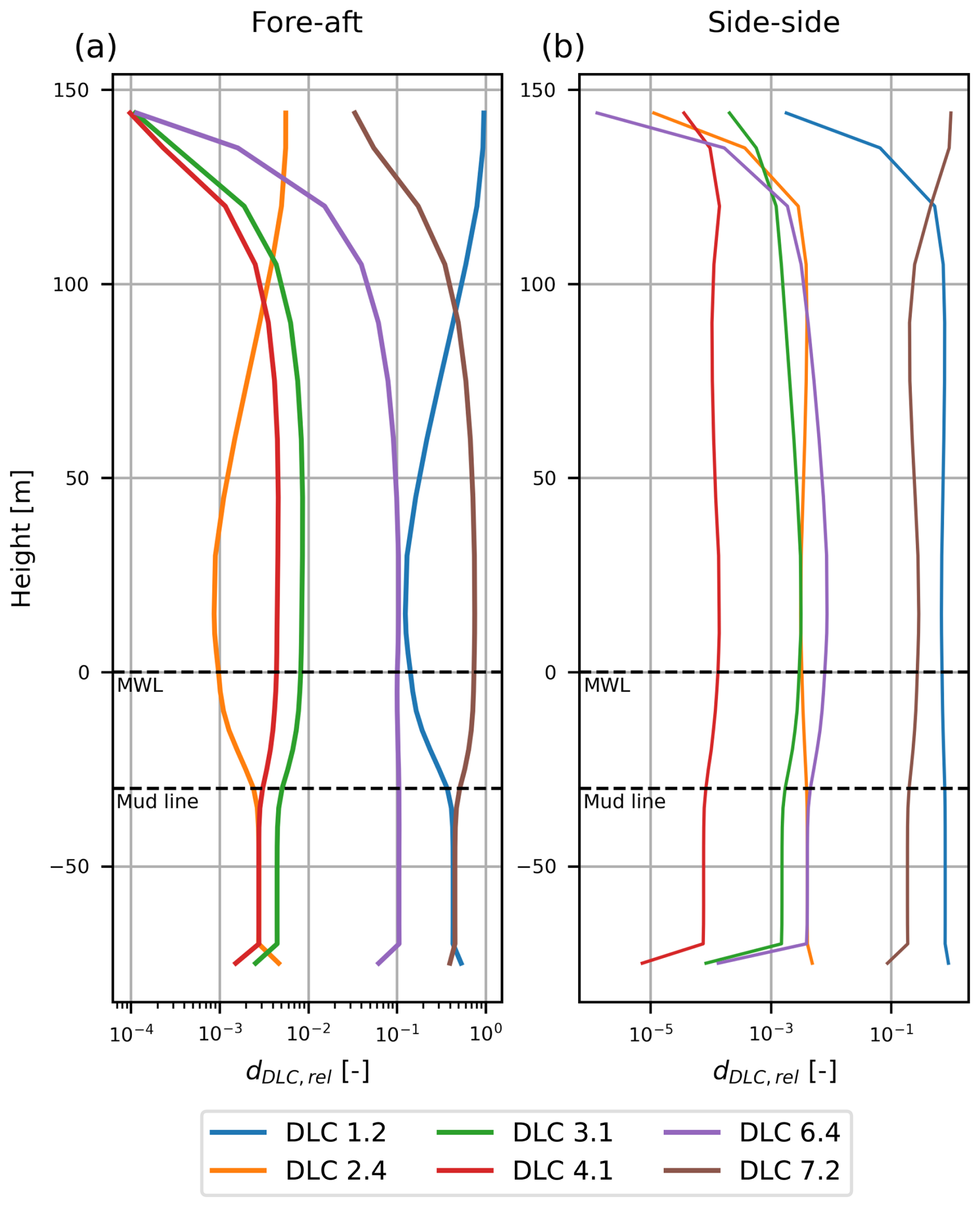
Figure 5 Relative damage for the individual DLCs calculated across the height of the IEA 15 MW RWT support structure as presented in Eq. (2) for the FA (a) and SS (b) directions.

From these relative damage plots in Fig. 5, it is observed that there is a big resemblance in the distribution of damage across the height of the IEA 15 MW RWT for DLCs 1.2 and 2.4, which is expected as these load cases are both for operation in normal conditions. A similar expected resemblance is found for DLCs 3.1 and 4.1, as these load cases represent start-up and shut-down, respectively. Figure 5a shows that approximately 99 % of the damage in the FA direction is caused by DLC 1.2 (power production in normal conditions), DLC 6.4 (parked – idle rotor in normal conditions), and DLC 7.2 (fault – locked rotor in normal conditions). In the SS direction, shown in Fig. 5b, the damage from DLC 6.4 falls below 1 %, so only DLCs 1.2 and 7.2 are considered significant for the damage in the SS direction. As presented in Table A3, DLC 1.2 is significantly more frequent than DLCs 6.4 and 7.2, and the significant damage contribution of this DLC is associated with the large duration, whereas for DLCs 6.4 and 7.2, the substantial damage contribution is associated with the large DELs (see Fig. 12).

The relative damage in the FA direction in Fig. 5a is dominated by DLC 1.2 at the tower top (≈100–144 m above the MSL). This is due to 3P effects (tower shadow, wind shear, and turbulence), which are significant contributors to damage in the tower top, as the varying forces on the blades and uneven loading on the rotor result in a significant moment at the hub. In the remainder of the free-standing support structure ($\approx -\mathrm{30}$–100 m), the relative damage in the FA direction is dominated by DLC 7.2. In this area, the section moments are governed to a higher degree by the global bending of the support structure caused by the thrust loading (for DLC 1.2) and especially the first tower FA mode (for DLCs 6.4 and 7.2). The tower bending modes in the FA direction for DLC 1.2 are subject to significant aerodynamic damping arising from the operating rotor, thus explaining the smaller contribution to the relative damage from this DLC and the larger contribution from DLCs 6.4 and 7.2, where the rotor does not operate and the aerodynamic damping is effectively negligible. Below MSL the relative damage contribution from DLCs 1.2 and 7.2 approaches each other and balances out at the mud line. This is likely due to the influence of wave loads, which increase with water depth and are less affected by the aerodynamic damping present for DLC 1.2.

The relative damage in the SS direction in Fig. 5b is dominated by DLC 7.2 at the tower top (≈120–144 m above MSL), while DLC 1.2 dominates the damage below this area. Unlike the FA response, the SS response for DLC 1.2 is not significantly affected by aerodynamic damping, the 3P effects, or the thrust load variations. Consequently, the damage in both DLC 1.2 and DLC 7.2 is primarily driven by ambient excitation at the turbine's resonant frequencies. However, the locked rotor condition in DLC 7.2 particularly influences damage at the tower top. Because the rotor is fixed in rotation and the blades are pitched 90°, the blades are more susceptible to turbulence-induced excitation, which creates a moment at the blade root. This, in turn, excites the second tower SS mode and possibly different rotor modes, resulting in DLC 7.2's dominant contribution to damage in the upper part of the support structure. In the lower part, the damage patterns are more governed by the first-order tower bending modes, which are similar for DLCs 1.2 and 7.2. However, the significantly longer duration of DLC 1.2 (90 % of the turbine's lifetime) results in it being dominant below 120 m. This effect is visible in Fig. 5b, where the distribution of relative damage from DLCs 1.2 and 7.2 remains rather constant in the support structure below 100 m, with d_DLC,rel for the two DLCs varying between 69 %–80 % and 19 %–29 %, respectively.

In conclusion, the damage in the support structure of the IEA 15 MW RWT is governed by both normal operation conditions and conditions where the rotor is idling or locked, whereas start-up and shut-down of the wind turbine and operation with yaw error are less critical. However, in a real operating scenario, shut-down and start-up may have a larger influence on the lifetime damage, as they occur more frequently than described by IEC (2019b) due to, for example, curtailment. This has not been accounted for in the present paper. The damage contribution across the elevation of the support structure arises from different local and global effects caused by different environmental and operational scenarios, e.g. turbulence, 3P effects, wave loads, and inherent dynamical properties. It should be emphasised that the durations used in this analysis for the DLCs are estimated, and scenarios can occur where the durations are differently distributed between the DLCs. Therefore, it is also relevant to evaluate DELs for individual DLCs, without accounting for their specific durations, when assessing how the different operational scenarios impact lifetime damage, as done in Sect. 5.2.

4 Virtual sensing

The present section initially explains the basic concepts of multi-band MDE and the methodology applied when moving from nodal displacements to internal force estimates. This is followed by a presentation of the prediction FE model used in the subsequent estimation of DELs and DESs in Sect. 5. Finally, the current section presents the model output with respect to dynamic mode shapes and quasi-static Ritz vectors.

4.1 Modal decomposition and expansion

Modal decomposition and expansion (MDE) is a well-established process model in virtual sensing (see Sect. 1). The formulation used in the present work is described in Iliopoulos et al. (2017). MDE assumes that the displacement vector u(t) of an undamped dynamic system can be decomposed and written as a linear combination of the system's mode shapes and modal coordinates on the matrix form:

$$\begin{array}{}\text{(5)}& \mathit{u}\left(t\right)=\mathbf{\Phi }\mathit{q}\left(t\right).\end{array}$$

The mode shape matrix $\mathbf{\Phi }=[{\mathit{\phi }}_{\mathrm{1}},{\mathit{\phi }}_{\mathrm{2}},\mathrm{\dots },{\mathit{\phi }}_n]$ contains the n mode shapes (φ_j) included to describe the dynamical system, while the modal coordinate vector $\mathit{q}\left(t\right)=\left[q_{\mathrm{1}}\right(t),q_{\mathrm{2}}(t),\mathrm{\dots },q_n(t){]}^{\mathrm{T}}$ collects the corresponding modal coordinates (q_j) at each time instant t. The mode shapes of the system φ_j can be derived from e.g. experimental or operational modal analysis, while in the present work, the vectors φ_j are derived from an FE model representing the dynamic system in Sect. 4.3. Assuming that the FE model is an accurate representation of the considered dynamic system, it follows that

$$\begin{array}{}\text{(6)}& \mathbf{\Phi }={\mathbf{\Phi }}_{\mathrm{FE}},\end{array}$$

which applies in the remainder of the paper. If the total number of degrees of freedom (DOFs) in the FE model is n_dof, the modal matrix Φ becomes an n_dof×n array. The nodal displacement vector u(t) in Eq. (5) is conveniently partitioned as

$$\begin{array}{}\text{(7)}& \mathit{u}\left(t\right)=\left[\begin{array}{c}{\mathit{u}}_{\mathrm{m}}\left(t\right)\\ {\mathit{u}}_{\mathrm{p}}\left(t\right)\end{array}\right]=\left[\begin{array}{c}{\mathbf{\Phi }}_{\mathrm{m}}\\ {\mathbf{\Phi }}_{\mathrm{p}}\end{array}\right]\mathit{q}\left(t\right),\end{array}$$

where the first n_m DOFs in u_m(t) represent those that are measured by physical sensors, while the remaining n_p DOFs in u_p(t) are those that are predicted by the MDE, i.e. the virtual sensors. By direct comparison of Eqs. (5) and (7), the mode shape matrix is similarly partitioned into

$$\begin{array}{}\text{(8)}& \mathbf{\Phi }=\left[\begin{array}{c}{\mathbf{\Phi }}_{\mathrm{m}}\\ {\mathbf{\Phi }}_{\mathrm{p}}\end{array}\right],\end{array}$$

in which the n_m×n array Φ_m refers to the mode shape amplitudes associated with the measured DOFs, while, correspondingly, the n_p×n array Φ_p accounts for the remaining DOFs that are used for the subsequent prediction procedure. From the above partitioning in Eqs. (7) and (8), it is seen that the total number of DOFs in the FE model is $n_{\mathrm{dof}}=n_{\mathrm{m}}+n_{\mathrm{p}}$, i.e. the sum of measured and predicted DOFs.

MDE utilises the fact that the displacements in u_m(t) are available from measurements, while the remaining DOFs in u_p(t) are predicted simultaneously once the modal matrix in Eq. (8) can be obtained from the underlying FE model with sufficient accuracy. It follows from Eq. (7) that the predicted nodal displacements can be expressed by the modal representation

$$\begin{array}{}\text{(9)}& {\mathit{u}}_{\mathrm{p}}\left(t\right)={\mathbf{\Phi }}_{\mathrm{p}}\mathit{q}\left(t\right).\end{array}$$

The modal coordinates in q(t), used for the extrapolation in Eq. (9), are determined by the corresponding relation

$$\begin{array}{}\text{(10)}& {\mathit{u}}_{\mathrm{m}}\left(t\right)={\mathbf{\Phi }}_{\mathrm{m}}\mathit{q}\left(t\right)\end{array}$$

for the measured DOFs in u_m(t). The inversion of this relation requires that the dynamic displacement field can be represented by at most n modes, where n must be less than or equal to the number of measured DOFs n_m. Hereby, the modal coordinates can be determined as

$$\begin{array}{}\text{(11)}& \mathit{q}\left(t\right)={\mathbf{\Phi }}_{\mathrm{m}}^{†}{\mathit{u}}_{\mathrm{m}}\left(t\right)\end{array}$$

using the Moore–Penrose pseudo-inverse depicted by the commonly used ( )^† symbol. The predicted nodal displacements are then obtained by substitution of Eq. (11) into Eq. (9), which then takes its final form

$$\begin{array}{}\text{(12)}& {\mathit{u}}_{\mathrm{p}}\left(t\right)={\mathbf{\Phi }}_{\mathrm{p}}{\mathbf{\Phi }}_{\mathrm{m}}^{†}{\mathit{u}}_{\mathrm{m}}\left(t\right).\end{array}$$

In virtual sensing, one of the objectives is to minimise the number of physical sensors n_m by introducing virtual sensors. Hence, the condition n ≤ n_m poses a challenge, as this limits the number of modes n that can be included to describe the dynamic system. Furthermore, for low frequencies, it can be desirable to perform MDE using only a subset of the measurements ${\stackrel{\mathrm{̃}}{\mathit{u}}}_{\mathrm{m}}\left(t\right)$ to minimise the noise introduced in the estimates or to introduce Ritz vectors containing static deflection shapes to predict the response u_p(t) in frequency ranges not dominated by resonant response (see Sect. 4.3.2). The introduction of multi-band virtual sensing in Iliopoulos et al. (2017) utilises the fact that the nodal displacement vector u(t) can be divided into separate bands B_i in the frequency domain, which, when combined by summation, reattains the original nodal displacement vector

$$\begin{array}{}\text{(13)}& \mathit{u}\left(t\right)=\sum _{i=\mathrm{1}}^N{\mathit{u}}_i\left(t\right)=\sum _{i=\mathrm{1}}^N{B}_i\left(\mathit{u}\right(t\left)\right),\end{array}$$

where u_i is the nodal displacement vector band-pass filtered in the band B_i, and $i=\mathrm{1},\mathrm{2}\mathrm{\dots }N$ denotes the individual frequency bands (see Fig. 11). Similarly, the predicted nodal displacements u_p(t) can be calculated in individual bands and combined by summation as

$$\begin{array}{}\text{(14)}& {\mathit{u}}_p\left(t\right)=\sum _i{\mathit{u}}_{i,p}\left(t\right)=\sum _i{\stackrel{\mathrm{̃}}{\mathbf{\Phi }}}_{i,p}{\stackrel{\mathrm{̃}}{\mathbf{\Phi }}}_{i,m}^{†}{\stackrel{\mathrm{̃}}{\mathit{u}}}_{i,m}\left(t\right),\end{array}$$

now only including the modes and Ritz vectors ${\stackrel{\mathrm{̃}}{\mathbf{\Phi }}}_i$ and the measurements ${\stackrel{\mathrm{̃}}{\mathit{u}}}_{\mathrm{m}}\left(t\right)$ that are relevant for the band B_i. This representation assumes that the energy content of u_p(t) is fully captured by the sum of its filtered components in the bands B_i.

4.2 Internal force estimation

Section 4.1 has explained how modal decomposition and expansion can be used to predict displacement response at virtual sensor locations. The present section extends the MDE to predict internal forces based on the predicted nodal displacement vector u_p(t).

The section forces to be predicted by the proposed method are specific to the element of the applied FE representation, e.g. bending moments for the planar beam elements used to describe the dynamics of the present support structure. Let the nodal forces be contained in the nodal element vector

$$\begin{array}{}\text{(15)}& \begin{array}{rl}{\mathbf{r}}_e\left(t\right)& ={\left[\begin{array}{c}{\mathbf{r}}_A\left(t\right)\\ {\mathbf{r}}_B\left(t\right)\end{array}\right]}_e={\left[\begin{array}{c}{f}_x^A\left(t\right),f_y^A\left(t\right),m^A\left(t\right),f_x^B\left(t\right),f_y^B\left(t\right),m^B\left(t\right)\end{array}\right]}_e^{\mathrm{T}}\\ & ={\left[\begin{array}{c}-N_A\left(t\right),V_A\left(t\right),-M_A\left(t\right),N_B\left(t\right),-V_B\left(t\right),M_B\left(t\right)\end{array}\right]}_e^{\mathrm{T}}\end{array}\end{array}$$

for a planar (2D) beam element e between two nodes A and B, with f_x, f_y, and m representing the nodal normal force, shear force and moment, respectively. As shown in Eq. (15), the corresponding section forces N, V, and M are derived from the nodal force by appropriate sign changes.

For a given element (subscript) e, the element nodal force vector in Eq. (15) can be determined by the element stiffness matrix k_e. The element stiffness relation can thus be written as

$$\begin{array}{}\text{(16)}& {\mathbf{r}}_e\left(t\right)={\mathbf{k}}_e{\mathbf{T}}_e{\mathit{u}}_{\mathrm{p}}\left(t\right),\end{array}$$

where T_e is a 6×n_p array that both collects and rotates the 6 DOFs from the global vector u_p(t) into the local coordinate system for element $e=\mathrm{1},\mathrm{2}\mathrm{\dots }{N}_e$. Elimination of the response in the predicted DOFs u_p(t) by Eq. (12) gives the compact representation

$$\begin{array}{}\text{(17)}& {\mathbf{r}}_e\left(t\right)={\mathbf{k}}_e{\mathbf{T}}_e{\mathbf{\Phi }}_{\mathrm{p}}{\mathbf{\Phi }}_{\mathrm{m}}^{†}{\mathit{u}}_{\mathrm{m}}\left(t\right)={\mathbf{D}}_e{\mathit{u}}_{\mathrm{m}}\left(t\right),\end{array}$$

where

$$\begin{array}{}\text{(18)}& {\mathbf{D}}_e={\mathbf{k}}_e{\mathbf{T}}_e{\mathbf{\Phi }}_{\mathrm{p}}{\mathbf{\Phi }}_{\mathrm{m}}^{†}\end{array}$$

defines the section force matrix that predicts the section forces r_e(t) from the measured nodal displacements in u_m(t). For a model with vertical beam elements, as in the present case, the transformation matrix T_e is an all-zero 6×n_p matrix, except for ±1 entries in the 6×6 block associated with the specific element e.

4.3 Prediction FE model

The prediction FE model from which the mode shapes and Ritz vectors used in the MDE are obtained is a 3D linear elastic beam model with the rotor nacelle assembly (RNA) and transition piece modelled as lumped inertias. The FE model is created using non-commercial Python-based FE software. The beam model is presented schematically in Fig. 6. The geometrical properties and the mass and stiffness input parameters for the prediction FE model are extracted from the HAWC2 model of the IEA 15 MW RWT described in Sect. A1 and presented in Appendix B.

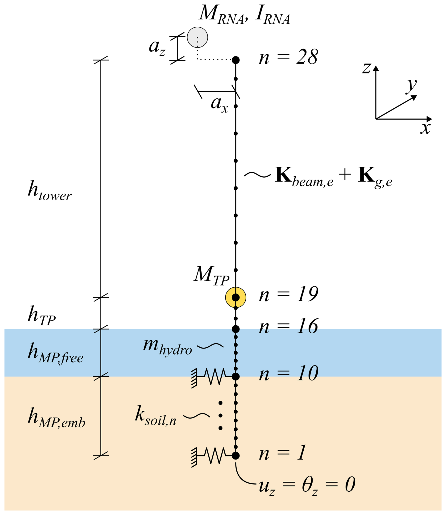
Figure 6 Schematic presentation of the prediction FE model used for the modal decomposition and expansion, including the height of the members in the support structure h_*, the element stiffness ${\mathbf{K}}_{\mathrm{beam},\mathrm{e}}+{\mathbf{K}}_{\mathrm{g},\mathrm{e}}$, the nodal masses of the transition piece M_TP and rotor nacelle assembly (RNA) M_RNA, the RNA inertia tensor I_RNA, the soil stiffness in node n k_soil,n, and the hydrodynamic added mass m_hydro.

The beam element stiffness is established according to Krenk and Høgsberg (2013), which combines the element stiffness matrix developed from the Timoshenko beam theory K_beam,e with a so-called geometric stiffness term K_g,e, expressing the total element stiffness matrix as

$$\begin{array}{}\text{(19)}& {\mathbf{K}}_e={\mathbf{K}}_{\mathrm{beam},\mathrm{e}}+{\mathbf{K}}_{\mathrm{g},\mathrm{e}},\end{array}$$

thus accounting for the stiffness contribution adhering from the normal forces causing Euler buckling in bending, although omitting the stiffness terms associated with torsion, i.e. loads causing lateral buckling in static analysis.

The monopile foundation support conditions are modelled using lateral linear elastic soil springs in the embedded part of the monopile. The stiffness of the individual springs k_soil,n varies with the embedment depth, as presented in Table A1. The bottom node in the beam model restrains torsion and vertical translation.

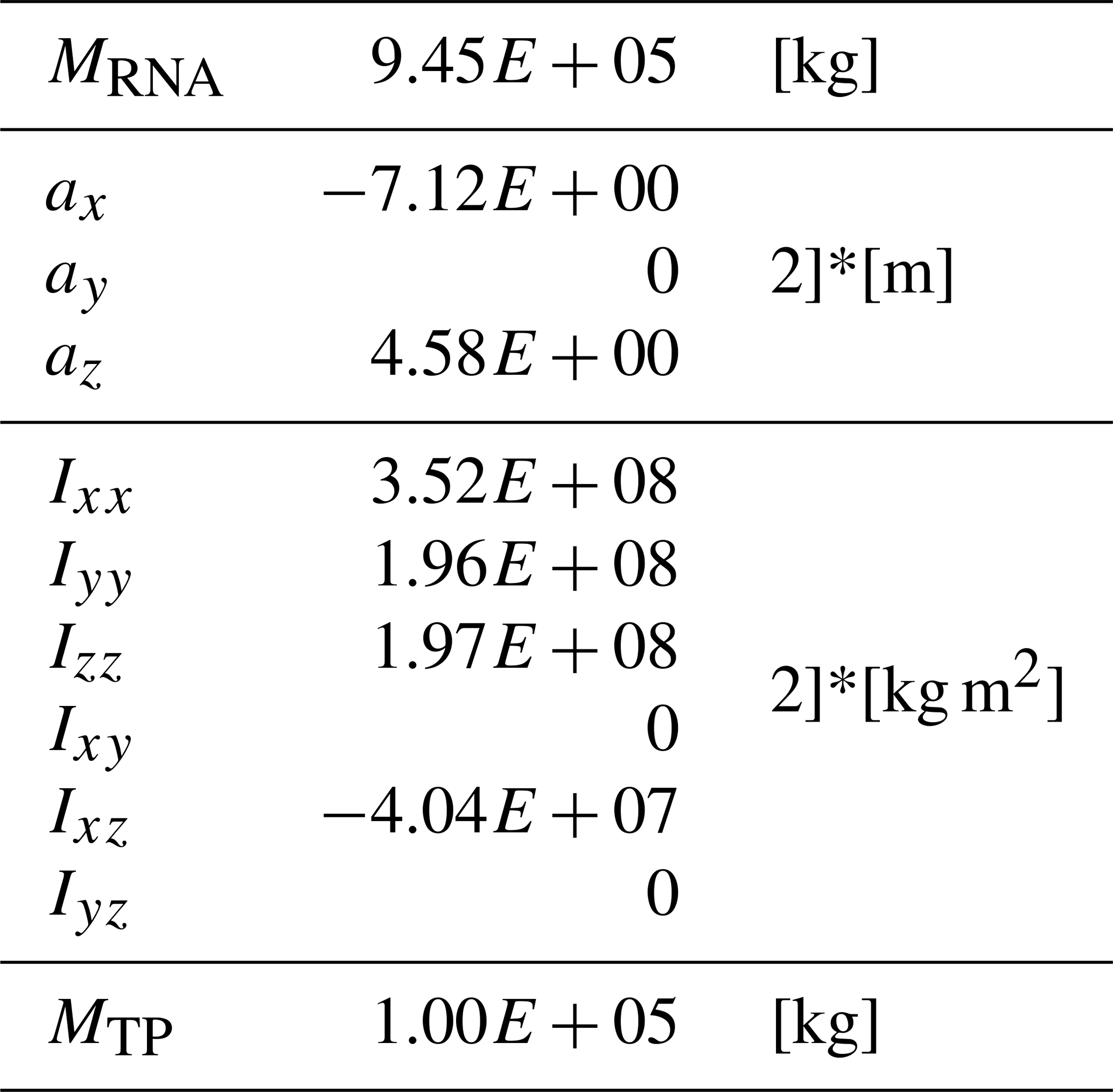
The mass contributing to the modal mass of the prediction FE model includes the distributed mass of the tower, transition piece, and monopile presented in Appendix B; the nodal mass of the transition piece M_TP located at the top of the transition piece; and the eccentric nodal mass and inertia tensor of the RNA, M_RNA and I_RNA, located at the distances a_x, a_y, and a_z relative to the top of the tower. The input parameters for the nodal masses for the TP and RNA and the mass moments and mass products of inertia included in the inertia tensor ($I_{xx},I_{yy},I_{zz},I_{xy},I_{xz},I_{yz},$) are presented in Table 1.

Table 1 Nodal mass, inertia tensor, and centre of gravity (CoG) of the IEA 15 MW RWT RNA, calculated based on the individual body properties extracted from HAWC2 and the nodal mass of the IEA 15 MW RWT transition piece (TP).

In addition to the mass contributions already presented, an external mass contribution, referred to as the hydrodynamic mass m_hydro, arises when a body moves in a fluid. According to Sumer and Fredsøe (1997), the hydrodynamic mass per unit length of a free circular cylinder can be expressed as

$$\begin{array}{}\text{(20)}& m_{\mathrm{hydro}}=\mathit{\rho }{C}_{\mathrm{m}}A\end{array}$$

if the current is disregarded. Here, the fluid density is ρ = 1027 kg m⁻³, C_m=1 is the hydrodynamic mass coefficient for a cylinder, and A = π r² is the fluid-displaced area for the monopile with radius r.

The first three tower bending mode shapes used for the MDE configuration in Sect. 5.1 have been calculated using the FE model presented above. They are shown in Fig. 7 for displacements and bending moments in the FA and SS directions.

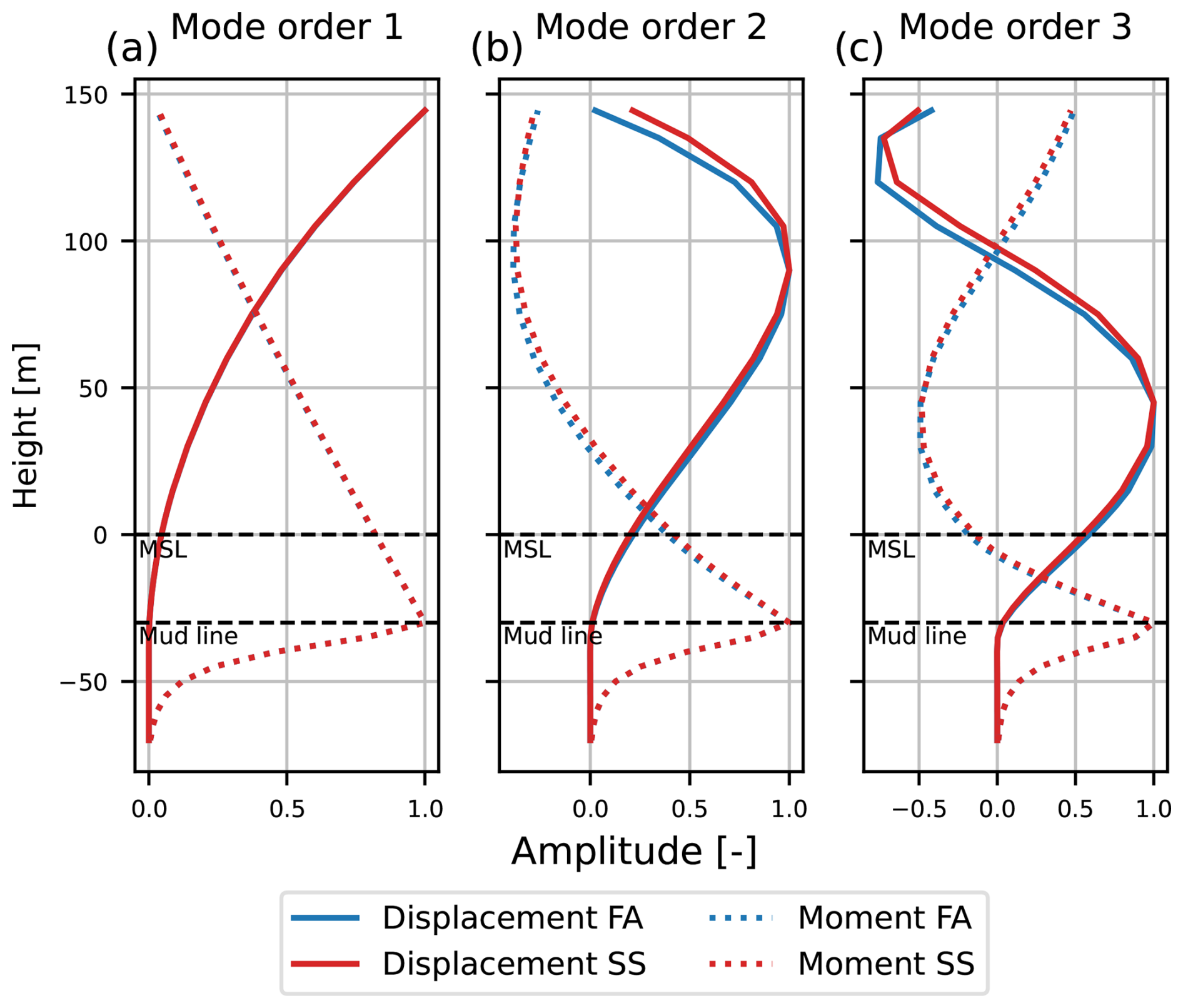
Figure 7 Mode shapes in terms of displacement and bending extracted from the prediction FE model presented in Fig. 6 in the FA and SS directions: (a) the first tower bending modes, (b) the second tower bending modes, and (c) the third tower bending modes.

4.3.1 Model validation

In the present section, the prediction FE model presented in Sect. 4.3 is validated. The validation is performed simply by comparing the undamped natural frequencies f_n of the prediction FE model to those of the IEA 15 MW RWT extracted using the HAWC2 built-in module system_eigenanalysis.

The objective of this validation is to ensure the correct interpretation of the input parameters derived from HAWC2 and used in the prediction FE model in Fig. 6. Therefore, this validation does not compare the prediction FE model against the full HAWC2 model of the IEA 15 MW RWT. Instead, the comparison is performed stepwise using the simplified HAWC2 model setups 1, 2, and 3 for the IEA 15 MW RWT, in which the rotor flexibility is deactivated so that the model comparison is performed accounting for the contributions to the mass and stiffness terms.

As mentioned previously, the prediction FE model does not include a detailed model of the RNA. Therefore, the influence of an operating rotor, blade flexibility, and shaft torsion is not included in the prediction FE model. In the simplified HAWC2 models, this is acknowledged by restraining shaft rotation, disabling torsional deformations, and using stiff blades. The comparison aims at validating the effects of mass and stiffness terms, soil support conditions, and hydrodynamic mass used in the prediction FE model by gradually adding these terms. This yields the following three model setups for the simplified HAWC2 model:

• Model setup 1. The hydrodynamic elements and the soil model are excluded, and the bottom node is fixed in all DOFs. This model resembles a bottom-fixed land-based wind turbine.

• Model setup 2. The hydrodynamic elements are excluded, while the soil support from the original HAWC2 model in Sect. A1 is reintroduced.

• Model setup 3. The hydrodynamic elements are introduced without water kinematics to reduce complexity.

The comparison of the natural frequencies of the simplified HAWC2 model f_n,HAWC2 and the prediction FE model f_n,Pred is presented for the first seven modes in Table 2, in which the error is calculated as

$$\begin{array}{}\text{(21)}& \mathit{\epsilon }\left(f_{\mathrm{n}}\right)={\displaystyle \frac{f_{\mathrm{n},\mathrm{Pred}}-f_{\mathrm{n},\mathrm{HAWC}\mathrm{2}}}{f_{\mathrm{n},\mathrm{HAWC}\mathrm{2}}}}.\end{array}$$

As presented in Table 2, the error ε(f_n) for the tower bending modes is within the range from −0.88 to 1.13 %, while for the torsion mode, the error range increases to 3.17 %–3.32 %. The two models are created from different underlying beam theories and implemented in different software tools, whereby discrepancies are expected. Thus, the agreement in Table 2 is generally good, with the larger error for the torsion mode possibly arising from the geometric stiffness matrix K_g,e in Eq. (19) not affecting torsional deformations.

Table 2 Overview of comparison of natural frequencies of the three different model setups for a simplified version of the IEA 15 MW RWT HAWC2 model and the prediction FE model presented in Sect. 4.3.

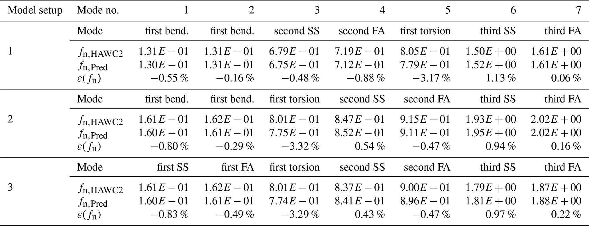
Based on the results in Table 2, it is concluded that the mass and stiffness terms and the soil model are reasonably implemented in the prediction FE model. Furthermore, the simple implementation of the hydrodynamic mass is deemed acceptable for cases where waves and currents are not included in the analysis. However, it is acknowledged that the model cannot capture the effects of currents and waves, as well as boundary effects at the seabed and water line. In the following sections, where the mode shapes used for the subsequent multi-band MDE are presented, only model setup 3 is considered, as it represents the most complete structural model that includes both soil support and hydrodynamic mass.

4.3.2 Ritz vectors

As explained in Sect. 4.1, the predicted response u_p(t) of a dynamic system can be estimated as the sum of the predicted response in the individual frequency bands B_i based on the mode shape matrix Φ. However, for large-scale OWTs, the quasi-static effects arising from e.g. yawing, wind, and waves significantly contribute to the response. These effects can be captured by a linear combination of higher-order modes. However, because a modal truncation omitting higher-order modes is needed in MDE, due to the limited number of sensors available, the accuracy of the predicted response may be compromised in the quasi-static region and between the resonant peaks. Different suggestions have been made to account for the quasi-static response, where Skafte et al. (2017) suggest the use of Ritz vectors. Similar methods are applied in Iliopoulos et al. (2017), Augustyn et al. (2021), and Toftekær et al. (2023). Furthermore, Tarpø (2020) compares the use of Ritz vectors with a modal truncation augmentation method and finds that the difference in performance is insignificant for the considered case. In the present work, the methodology using Ritz vectors based on static loads from Skafte et al. (2017) is applied, as explained in the following.

The mode shape matrix in Eq. (8) is extended to include not only the n mode shapes of the dynamic system Φ_d obtained from the eigenanalysis of the FE model presented in Sect. 4.3, but also the m Ritz vectors obtained from static analysis Φ_s:

$$\begin{array}{}\text{(22)}& \mathbf{\Phi }=\left[\begin{array}{c}{\mathbf{\Phi }}_{\mathrm{s}}{\mathbf{\Phi }}_d,\end{array}\right]\end{array}$$

whereby Φ becomes an $n_{\mathrm{dof}}\times (m+n)$ array. The matrix ${\mathbf{\Phi }}_{\mathrm{s}}=[{\mathit{\varphi }}_{\mathrm{1}},{\mathit{\varphi }}_{\mathrm{2}},\mathrm{\dots },{\mathit{\varphi }}_m]$ contains the m Ritz vectors (ϕ_k), obtained by the static solution

$$\begin{array}{}\text{(23)}& {\mathbf{\Phi }}_{\mathrm{s}}={\mathbf{K}}^{-\mathrm{1}}\mathbf{F},\end{array}$$

where K is the stiffness matrix of the FE model presented in Fig. 6, and F contains the static load vectors f_i, representing the load effects included in the MDE. Both Toftekær et al. (2023) and Iliopoulos et al. (2017) suggest that an appropriate Ritz vector for the thrust load can be obtained by applying a horizontal nodal force at the top of the FE model tower; see Fig. 8a. Furthermore, Toftekær et al. (2023) show that a supplemental Ritz vector from the nodal tower top moment in Fig. 8b improves the MDE strain estimates associated with RNA yaw or uneven rotor loading. Finally, Skafte et al. (2017), Tarpø (2020), and Augustyn et al. (2021) all include load from waves in the performed MDE; see Fig. 8c. In the present work, three pairs of Ritz vectors are included in the MDE, representing the FA and SS directions. In each direction, the tower top nodal load (Fig. 8a) and moment (Fig. 8b) and the wave loading (Fig. 8c) are presented in Fig. 8. A Ritz vector for the distributed wind load on the tower has not been established in the present work. However, as presented in Table 3, the first tower bending mode shapes are used to represent the quasi-static response resulting from this load.

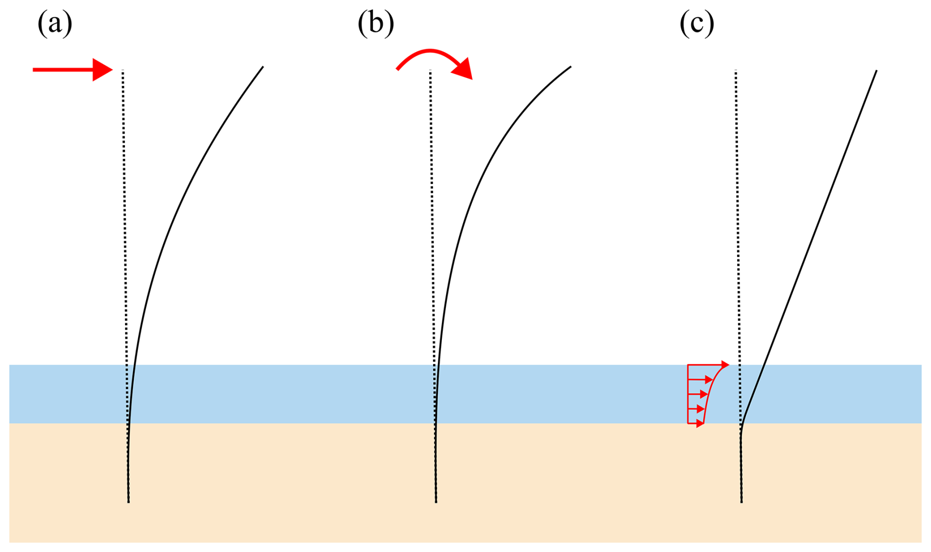
Figure 8 Loads and moments applied to determine the Ritz vectors for the estimation of the quasi-static response. Based on suggested loads in Toftekær et al. (2023). Panel (a) shows the tower top nodal load, (b) shows the tower top moment, and (c) shows the wave loading.

The wave load depicted in Fig. 8c is based on the expression for the total force

$$\begin{array}{}\text{(24)}& F_x(z,t)={\displaystyle \frac{\mathrm{2}\mathit{\rho }gH}{k}}{\displaystyle \frac{\cosh \left(k\right(z+h\left)\right)}{\cosh \left(kh\right)}}A\left(k{r}_{\mathrm{0}}\right)\cos (\mathit{\omega }t-\mathit{\delta })\end{array}$$

on a unit height of a vertical cylinder (Sumer and Fredsøe, 1997). In the present work, normalised displacements are used. Hence, only the distribution across the water depth of the monopile is of interest, whereby the temporal and constant terms can be removed in Eq. (24). Thereby, the vertical distribution of the force (above the seabed) is reduced to

$$\begin{array}{}\text{(25)}& F_x^{\prime }\left(z\right)={\displaystyle \frac{\cosh \left(k\right(z+h\left)\right)}{\cosh \left(kh\right)}},\end{array}$$

where h=30 m is the water depth, and $k=\frac{\mathrm{2}\mathit{\pi }}{L}$ is the deep-water wave number, derived for the wave length $L=\frac{g}{\mathrm{2}\mathit{\pi }}{T}^{\mathrm{2}}$ with the wave period T = 6.52 s calculated for a hub wind speed of V_hub=10 m s⁻¹. The distributed force in Eq. (25) assumes that the wave loads are dominated by the inertia contribution in Morison's equation, while neglecting drag. This assumption is indeed valid for V_hub=10 m s⁻¹, for which inertia forces constitute 98.5 % of the total force. However, extending the wave load Ritz vector to be wind speed dependent might be relevant, as suggested in Tarpø (2020). The Ritz vectors obtained from the load presented in Fig. 8 are presented in Fig. 9 in terms of displacements and bending moments.

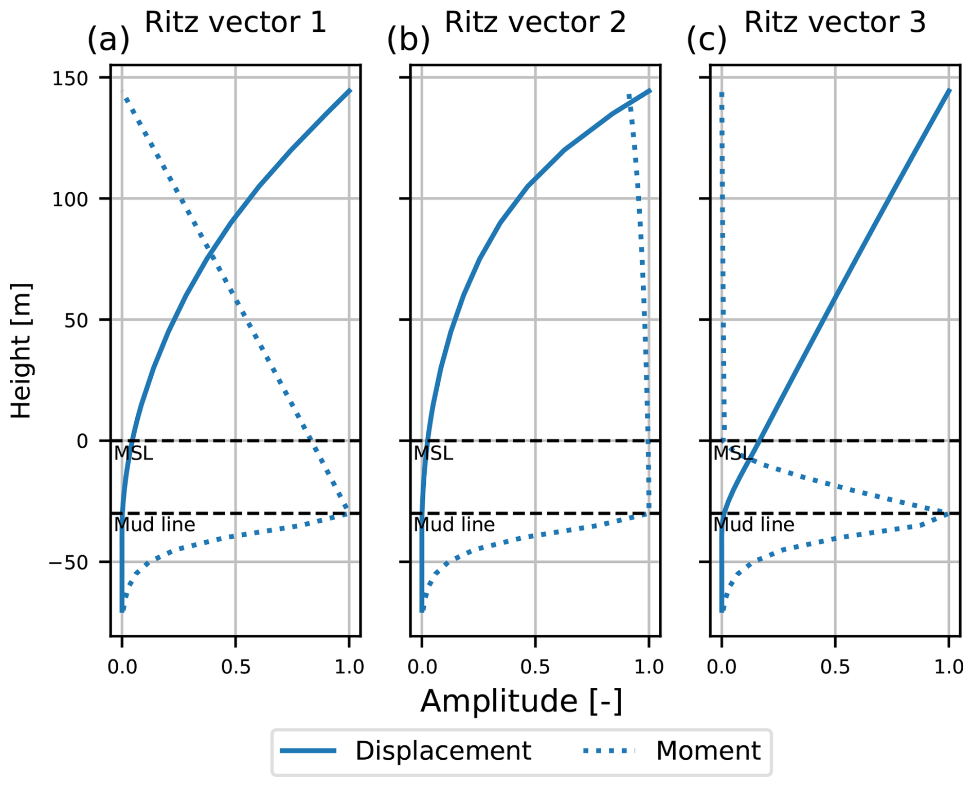
Figure 9 Ritz vectors in terms of displacement and bending moments extracted from the prediction FE model presented in Fig. 6: (a) is based on the nodal force in the tower top, (b) is based on the nodal moment in the tower top, and (c) is based on the approximated wave load presented in Eq. (25). The three loads are illustrated in Fig. 8.

5 MDE estimation of damage equivalent loads and stresses

The objective of the multi-band MDE is to obtain valid estimates of strains, stress, or force histories at any given location in a given structure. The accuracy of the MDE depends not only on the quality of the FE model from Sect. 4.3, but also on the configuration and input data, which are presented in Sect. 5.1. The purpose of the applied multi-band MDE is to evaluate the fatigue damage from bending stresses in any relevant location of the support structure. Hence, the performance of the MDE should be assessed using a measure that accounts for the accuracy in terms of strains or forces, while also being consistent with how fatigue damage is evaluated. In Sect. 5.2 this comparison is therefore conducted in terms of DELs and DESs.

5.1 MDE setup

This section presents the basis for the MDE performed for the IEA 15 MW RWT support structure in terms of sensor type and placement (i.e. the HAWC2 output channels in u_m(t)), band separation used in the frequency domain, and the choices of Ritz vectors and mode shapes used within the individual bands (${\stackrel{\mathrm{̃}}{\mathbf{\Phi }}}_i$).

As presented in Sect. 1, it is widely accepted in the literature that the dynamic part of the response u_p(t) can be predicted based on measured accelerations. From these accelerations, displacements are obtained through double integration. However, for the quasi-static part of the response, the displacements are often inaccurate because measurement noise in the acceleration measurements is amplified during low-frequency integration. To overcome this challenge, Iliopoulos et al. (2017) use strain gauge measurements as input to the MDE for the quasi-static response estimation. Alternatively, Toftekær et al. (2023) use the low-pass-filtered (vertical) accelerations obtained from DC accelerometers relative to the gravitational acceleration to estimate rotations. This has the advantage that no double integration must be performed, and no additional sensors must be installed. In the present work, u_m(t) therefore contains displacements and rotations for the prediction of dynamic and quasi-static responses, respectively (see Fig. 10).

Obviously, the location of the accelerometers will impact the quality of the virtual sensors. Different methods have been used to optimise the sensor placement (Mehrjoo et al., 2022; Ercan and Papadimitriou, 2021). However, in practical applications, accessibility is just as relevant for the installation of sensors, since maintenance and replacement of structural health monitoring systems play a central role in the robustness of the overall system. Thus, in the present work, the physical sensors are placed at locations where internal platforms are most likely installed inside the tower (see Fig. 10).

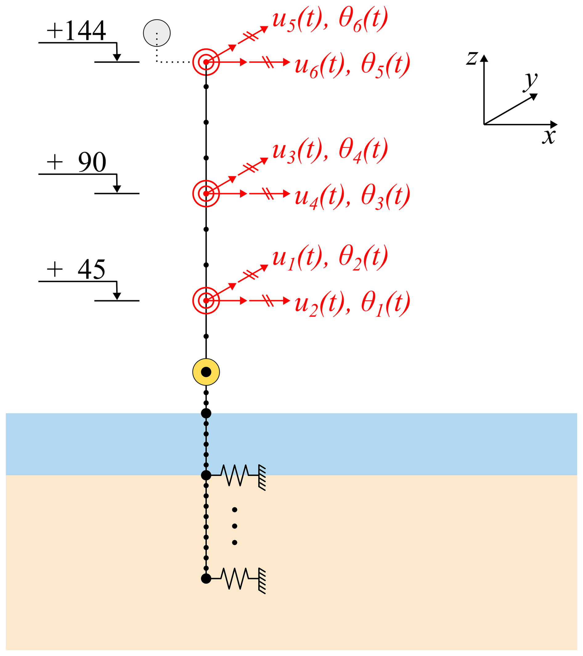
Figure 10 Measurement locations, i.e. HAWC2 output channels in red in terms of displacements u_*(t) included in MDE in dynamic frequency range and rotations θ_*(t) included in MDE in quasi-static frequency range.

As presented in Fig. 11, the multi-band MDE in Eq. (14) is performed by separating the response of the IEA 15 MW RWT into four individual bands (B₁ to B₄) before combining them into the total predicted response u_p(t).

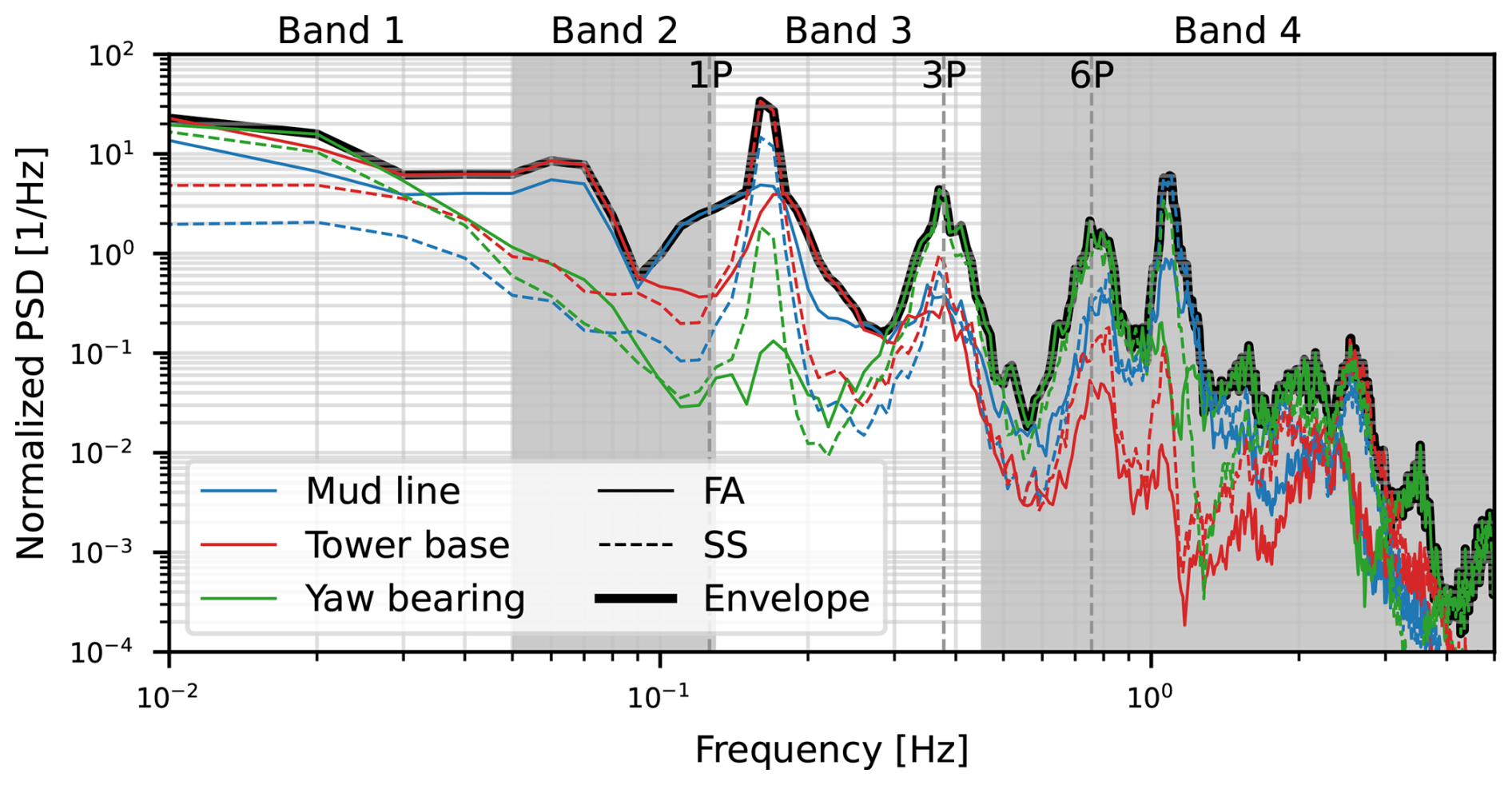
Figure 11 Normalised PSD of moment time series (from DLC 1.2). The frequency spectra of the moments at the yaw bearing, tower base, and mud line are shown in the FA and SS directions. Transparent white/grey bands indicate the frequency ranges used in the MDE, representing Band 1 (turbulence), Band 2 (turbulence and wave loads), Band 3 (first tower bending and wave loads), and Band 4 (higher dynamic modes and rotor harmonics).

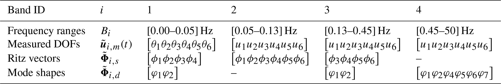
The rationale for the band separation depends on case-specific factors, including the frequency distribution of the external loads, the dynamic properties of the considered structure, and the properties of the sensors available in the monitoring system. Thus, the frequency bands should be selected such that the response is predicted accurately without exceeding the inherent sensor limitations of the MDE. The justification of the present band separation is given below for the MDE configuration summarised in Table 3:

• B₁ is defined with an upper limit of 0.05 Hz. According to Toftekær et al. (2023), accurate displacements cannot be obtained from measured accelerations at frequencies below 0.05 Hz. Hence, the measured DOFs in Φ_m are defined in terms of rotations in B₁, and the boundary represents a practical limitation of the sensors. B₁ represents the quasi-static domain of the response, primarily driven by turbulence. Thus, the Ritz vectors included for the prediction in this band are obtained from the nodal force and moment in Fig. 8a and b. Furthermore, the wind is assumed to act as a distributed load across the tower, whereby the first tower bending mode shapes in Fig. 7a are also included in the MDE.

• B₂ is defined within the frequency range 0.05 to 0.13 Hz. The upper limit is chosen as the boundary between the thrust-dominated and the resonant parts of the response, dominated by the first tower bending modes. B₂ is governed by wave loading with a wave frequency of $\mathrm{1}/T_{\mathrm{p}}=\mathrm{0.068}$ Hz at V = 35 m s⁻¹ and $\mathrm{1}/T_{\mathrm{p}}=\mathrm{0.18}$ Hz at V = 4 m s⁻¹ for the given site conditions. Furthermore, the wind load also contributes significantly to the response in this frequency band, whereby all three pairs of Ritz vectors in Fig. 9 are included in the MDE for this band.

• B₃ is defined within the frequency range 0.13 to 0.45 Hz. The upper limit is defined as the boundary between the 3P frequency and the frequency of the first flapwise blade mode. B₃ is governed by the first tower bending modes along with the wave loads and the 3P excitation. Hence, the first tower bending mode shapes in Fig. 7a and the Ritz vectors from wave loading in Fig. 8c are included in the MDE. As the 3P excitation is driven primarily by uneven thrust loading on the rotor, it is well represented by the Ritz vector obtained from a nodal moment in Fig. 8b; hence, the Ritz vector in Fig. 9b is also included in B₃ for the MDE.

• B₄ is defined within the frequency range 0.45 to 50 Hz. This frequency band represents a part of the response where the external loads are of minor influence. Hence, B₄ includes the higher-order dynamics and rotor harmonics. Here, the first three pairs of tower bending modes in Fig. 7 are included in the MDE, while the first tower torsion mode is omitted as it is considered less significant for estimating bending stresses.

The following section assesses the performance of the MDE using the configuration described above and the prediction FE model presented in Sect. 4.3. This is achieved by comparing DELs and DESs, calculated from section moment load histories, obtained from both the MDE and the true HAWC2 output time series. The comparison is performed in both the FA and the SS directions and at all nodes in the support structure for the DLCs described in Sect. A3.

Table 3 Configuration used for the multi-band MDE in Eq. (14) in the band frequency ranges B₁, B₂, B₃, and B₄. The configuration is defined in terms of measured DOFs u_i,m(t) (Fig. 10), Ritz vectors (Fig. 9), and mode shapes (Fig. 7) applied within the individual bands.

5.2 Damage equivalent loads and stresses

Fatigue DELs reduce a load history to a single equivalent load range ΔP_eq, which is defined as the constant amplitude 1 Hz sinusoidal load causing the same amount of fatigue damage as the original load history. The same applies to fatigue DESs ΔS_eq, making DELs and DESs convenient measures of comparing fatigue contributions across load cases with different durations (Veldkamp, 2006). Thus, in the present section, the DELs and DESs combined for the individual DLCs presented in Sect. A3 are compared and discussed. Furthermore, the MDE performance is assessed: first for DELs and DESs calculated for the individual DLCs and, subsequently, in Sect. 5.3, for the DESs calculated for the individual HAWC2 section moment time histories. In both cases, the comparison is performed in all nodes of the IEA 15 MW RWT HAWC2 model.

The DEL for a single load history ΔP_eq,s can be calculated as in Eq. (4), where n_eq is the number of 1 Hz cycles in the considered time series. Similarly, the DEL for the individual DLCs can be calculated as

$$\begin{array}{}\text{(26)}& \mathrm{\Delta }{P}_{\mathrm{eq},\mathrm{DLC}}={\left({\displaystyle \frac{{\sum }_{\mathrm{s}\in \text{DLC}}{n}_{\mathrm{eq}}(\mathrm{\Delta }{P}_{\mathrm{eq},\mathrm{s}}{)}^m}{n_{\mathrm{eq},\mathrm{DLC}}}}\right)}^{\frac{\mathrm{1}}{m}},\end{array}$$

where

$$\begin{array}{}\text{(27)}& n_{\mathrm{eq},\mathrm{DLC}}=n_{\mathrm{eq}}{n}_{\mathrm{seed},\mathrm{DLC}}\end{array}$$

is the total number of 1 Hz cycles in the simulations contained in the individual DLCs, with n_seed,DLC being the simulation seeds for the individual DLC (i.e. the number of (converged) simulations in Table A2 for a given DLC at MWL equal to MSL). Inserting Eq. (27) in Eq. (26) yields the more compact representation

$$\begin{array}{}\text{(28)}& \mathrm{\Delta }{P}_{\mathrm{eq},\mathrm{DLC}}={\left({\displaystyle \frac{{\sum }_{\mathrm{s}\in \text{DLC}}(\mathrm{\Delta }{P}_{\mathrm{eq},\mathrm{s}}{)}^m}{n_{\mathrm{seed},\mathrm{DLC}}}}\right)}^{\frac{\mathrm{1}}{m}}.\end{array}$$

As the DEL retains the unit of the load, the DES ΔS_eq,s can be obtained by applying Navier's stress distribution formula to the DEL ΔP_eq,s for the individual nodes of interest in the support structure. However, the elements in the IEA 15 MW RWT are not consistent in terms of bending stiffness across the nodes, whereby Navier's formula will produce discontinuous stresses at the nodes. Thus, only the DES associated with the maximum nodal stresses in the monopile and tower circumference are considered for each node. Furthermore, only the contributions arising from the bending moments are included in the DESs, which are calculated as

$$\begin{array}{}\text{(29)}& \mathrm{\Delta }{S}_{\mathrm{eq},\mathrm{DLC}}={\left({\displaystyle \frac{{\sum }_{\mathrm{s}\in \text{DLC}}(\mathrm{\Delta }{S}_{\mathrm{eq},\mathrm{s}}{)}^m}{n_{\mathrm{seed},\mathrm{DLC}}}}\right)}^{\frac{\mathrm{1}}{m}}\end{array}$$

for the individual DLCs.

Figures 12 and 13 show the DELs and DESs related to the FA and SS section moments obtained from the HAWC2 simulations directly (solid line) and predicted using the multi-band MDE configuration from Sect. 5.1 (dashed line).

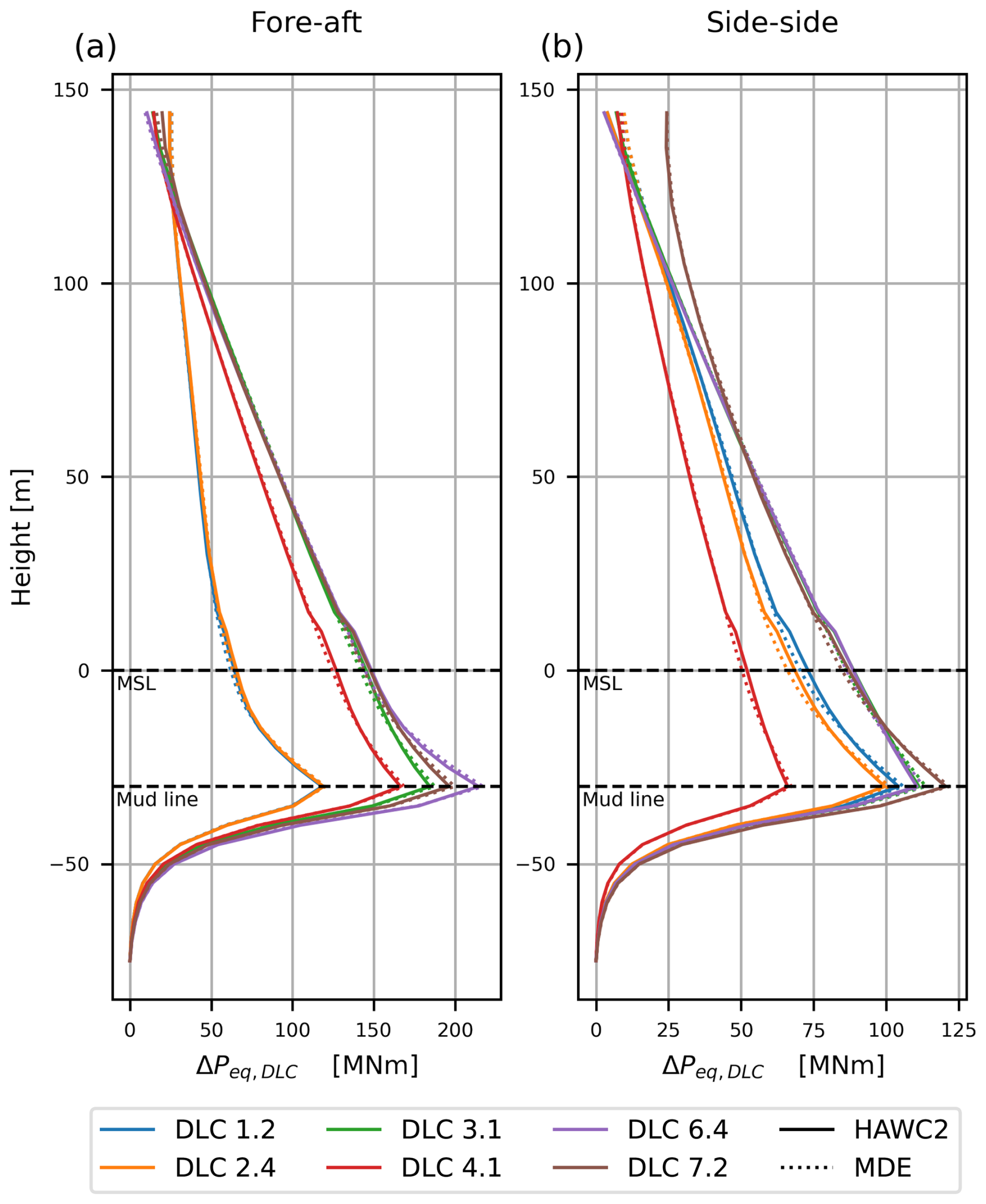
Figure 12 DELs calculated for the individual DLCs based on section moment load histories from HAWC2 (solid line) and MDE prediction (dashed line) in the FA (a) and SS (b) directions of the IEA 15 MW RWT, as presented in Eq. (28).

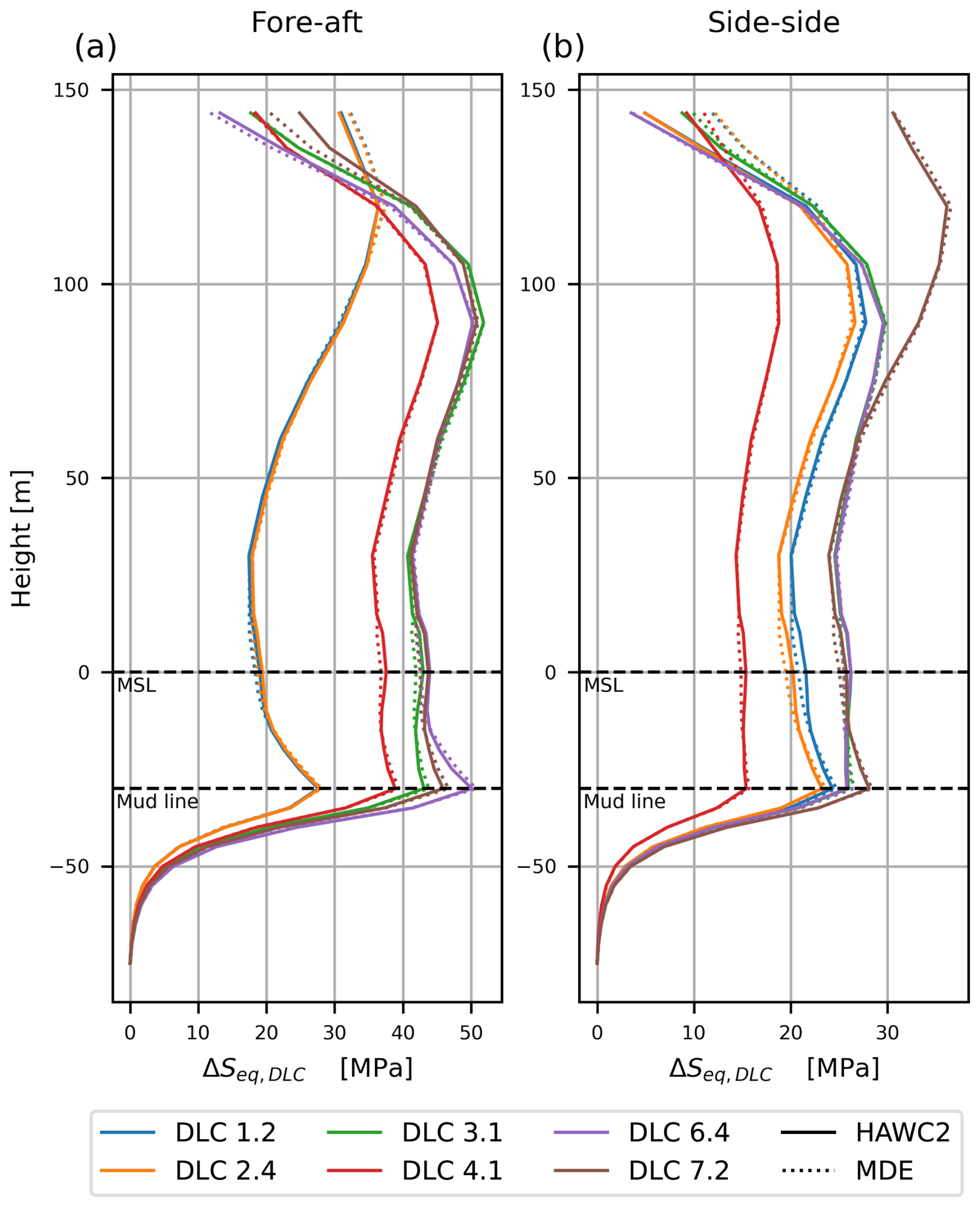
Figure 13 DESs calculated for the individual DLCs based on section moment load histories from HAWC2 (solid line) and MDE prediction (dashed line) in the FA (a) and SS (b) directions of the IEA 15 MW RWT, as presented in Eq. (29).

As illustrated in Fig. 12, the DELs generally look similar to the moment curve from the first tower bending modes or the thrust load (see Figs. 7 and 9), with overlying effects from other loads and modes. In the FA direction (a), the operating DLCs 1.2 and 2.4 generally induce lower DELs compared to DLCs 3.1, 4.1, 6.4, and 7.2, with DLC 6.4 resulting in the maximum DEL across all DLCs and directions (FA and SS) at the mud line. The lower DELs of DLCs 1.2 and 2.4 can be attributed to the significant aerodynamic damping provided by the operating rotor, as discussed in Sect. 3.2. However, within the tower top region, specifically from around 120–144 m, the operating DLCs show higher DELs due to uneven loading of the rotor and 3P effects, as discussed in Sect. 3.2.

In the SS direction (b), in which the aerodynamic damping, the effects from thrust load variations, and the 3P effects have less influence, the differences in DEL between operating and non-operating DLCs are generally smaller than those observed in the FA direction (a). It is worth noting that DLC 7.2 results in significantly higher DELs than all other DLCs at elevations above approximately 75 m. As discussed in Sect. 3.2, this can be attributed to tower top moment arising from the blade vibrations, which are enabled by the locked rotor configurations specific to this DLC.

An inherent problem of the DELs in Fig. 12 is that they do not explicitly account for changes in cross-section dimensions, whereby small DELs might still cause large stresses in regions with small tower diameters. Thus, in Fig. 13, the DESs have large values in the tower top region, where the corresponding DELs in Fig. 12 are small. This indicates that the accuracy of the MDE cannot be ignored in the tower top region. For the present analysis in Fig. 13, this is especially important for DLCs 1.2 and 2.4 in the FA direction (a) and DLC 7.2 in the SS direction (b), which have their DES maxima in the tower top region.

Figures 12 and 13 show that the MDE underestimates the DELs in a ±15 m zone around the MSL for all DLCs in both the FA and the SS directions. Furthermore, for the DESs estimated by MDE in Fig. 13, it is seen that the multi-band MDE performs poorly at the tower top, where it overestimates the DESs of the operating DLCs (1.2 and 2.4) in both the FA and the SS directions while underestimating the DESs for the standstill DLCs (6.4 and 7.2) in the FA direction.

5.3 MDE performance

Figures 12 and 13 are based on a combined DEL and DES calculated for the individual DLCs for each elevation z along the IEA 15 MW RWT support structure. Thus, it corresponds to an averaged or mean error, conveniently used for assessing long-term MDE performance, although inherently sensitive to bias errors. Therefore, to assess the short-term performance of the MDE in the individual HAWC2 simulations, the relative error of the DESs is calculated for the individual HAWC2 simulations as

$$\begin{array}{}\text{(30)}& {\mathit{\epsilon }}_{\mathrm{MDE}}={\displaystyle \frac{\mathrm{\Delta }{S}_{\mathrm{eq},\mathrm{s},\mathrm{MDE}}}{\mathrm{\Delta }{S}_{\mathrm{eq},\mathrm{s},\mathrm{HAWC}\mathrm{2}}}}-\mathrm{1},\end{array}$$

where ( )_HAWC2 denotes the DESs calculated from the HAWC2 time series of the FA and SS section moments, and ( )_MDE denotes the DESs calculated from the corresponding MDE estimate. Figure 14 presents the relative error ε_MDE of the DESs, related to the FA and SS section moment and calculated for each elevation z along the IEA 15 MW RWT support structure.

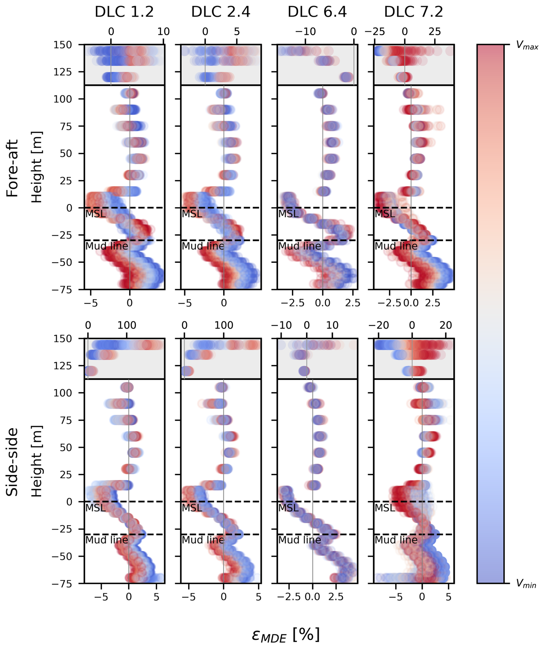
Figure 14 Error ε_MDE of DESs for the MDE-predicted section moment load histories in the FA (top) and SS (bottom) directions of the IEA 15 MW RWT from the individual HAWC2 simulation s, as presented in Eq. (30). Colour gradient represents the mean wind speed at the hub V_hub for the considered simulation s. Two separate x axes are used to present ε_MDE (illustrated with white and grey background colour).

It is observed in Fig. 14 that the error ε_MDE is predominantly in the range of ±5 %, except at the tower top, where the MDE performs inconsistently for the various DLCs. The error generally shows a dependency on the wind speed, which can be attributed to the operational and environmental variability of the IEA 15 MW RWT, arising from the varying rotor speeds, changing turbulence, and changing wave loads, which cannot be captured by the MDE, assuming a linear and time-invariant response.

In the following sections, the tower top MDE error observed in Figs. 13 and 14 is discussed for the individual operating scenarios (operating, idle, and locked rotor). Furthermore, the MDE error observed at ±15 m around MSL in Figs. 12 and 13 is discussed. To contextualise the behaviour observed in Figs. 12 to 14 and enhance insight into the discrepancies between the DELs and DESs obtained from HAWC2 and MDE, selected sample moment histories are considered in the discussion. These are chosen based on the error metric ε_MDE; however, for DLC 7.2, the sample moment histories have been chosen based on the absolute error obtained from

$$\mathrm{\Delta }{S}_{\mathrm{eq},\mathrm{s},\mathrm{MDE}}-\mathrm{\Delta }{S}_{\mathrm{eq},\mathrm{s},\mathrm{HAWC}\mathrm{2}}.$$

Intervals of the selected moment histories discussed in the following sections are presented in Appendix C

5.3.1 DLCs 1.2 and 2.4: MDE error at tower top

In the present section, the MDE error (ε_MDE) at the tower top elevation from 135–144 m (Figs. 13 and 14) is considered for the operating DLCs (1.2 and 2.4). As previously mentioned, Fig. 13 shows that the MDE generally overestimates the DES for DLCs 1.2 and 2.4, which is most pronounced in the SS direction (b). This is underlined by Fig. 14, which shows that the maximum MDE error for DLCs 1.2 and 2.4 is approximately 10 % in the FA (top) direction, while reaching approximately 188 % in the SS (bottom) direction for DLC 1.2, with similar errors observed for DLC 2.4.

To contextualise the behaviour observed in Figs. 13 and 14, the moment histories from DLC 1.2 corresponding to the five largest MDE errors at an elevation of 144 m in the FA and SS directions, respectively, have been selected for further analysis. Figures C1 and C2 present segments of the moment histories, while Figs. 15 and 16 provide an overview of the moment response in terms of the PSDs of the HAWC2 moment histories, the difference between the HAWC2- and MDE-predicted moment histories, the wind speed, and the wave amplitude for this selection.

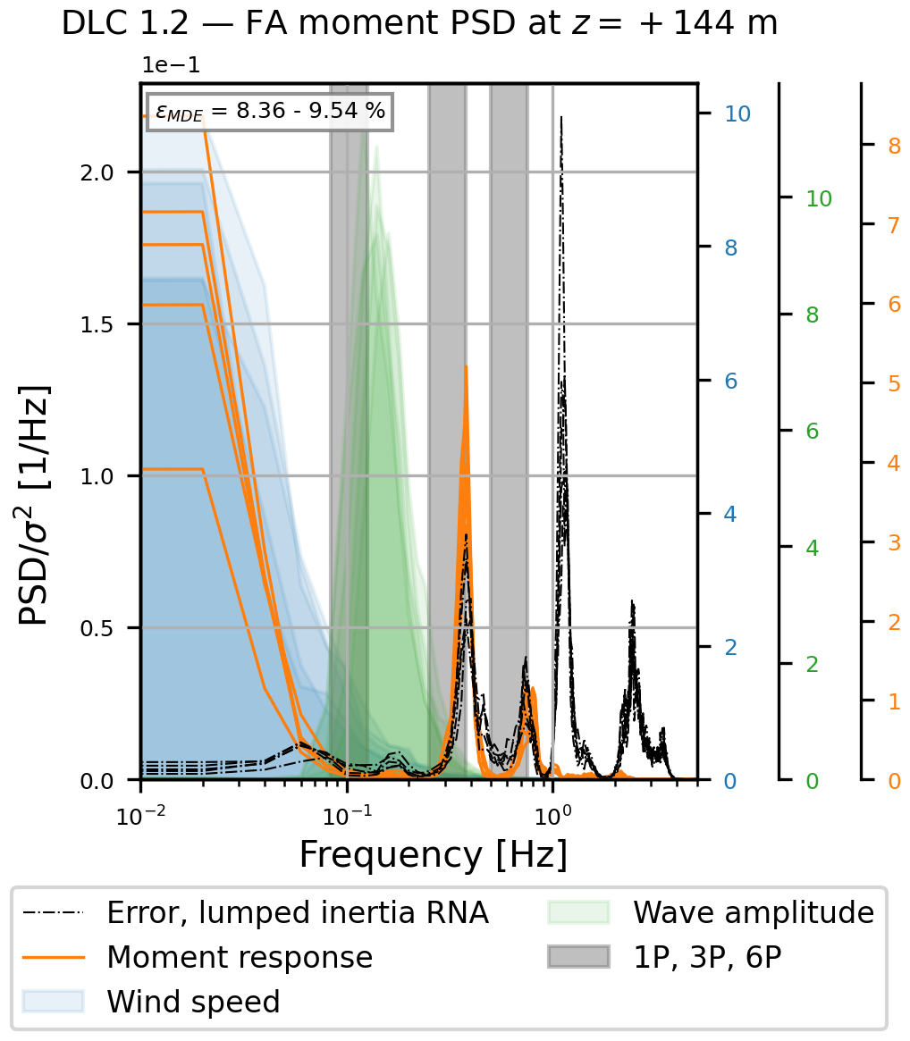
Figure 15 Normalised PSDs representing the MDE performance for the FA moment at the 144 m elevation for five selected moment histories in DLC 1.2. The corresponding selected moment histories are presented in Fig. C1. The PSDs include (1) the MDE error for the lumped-inertia RNA model (black), (2) the 10 min section moment time series (orange), (3) the wind speed in the FA direction (light blue), and (4) the wave amplitude (green). The grey bands indicate the 1P, 3P, and 6P excitation frequencies.

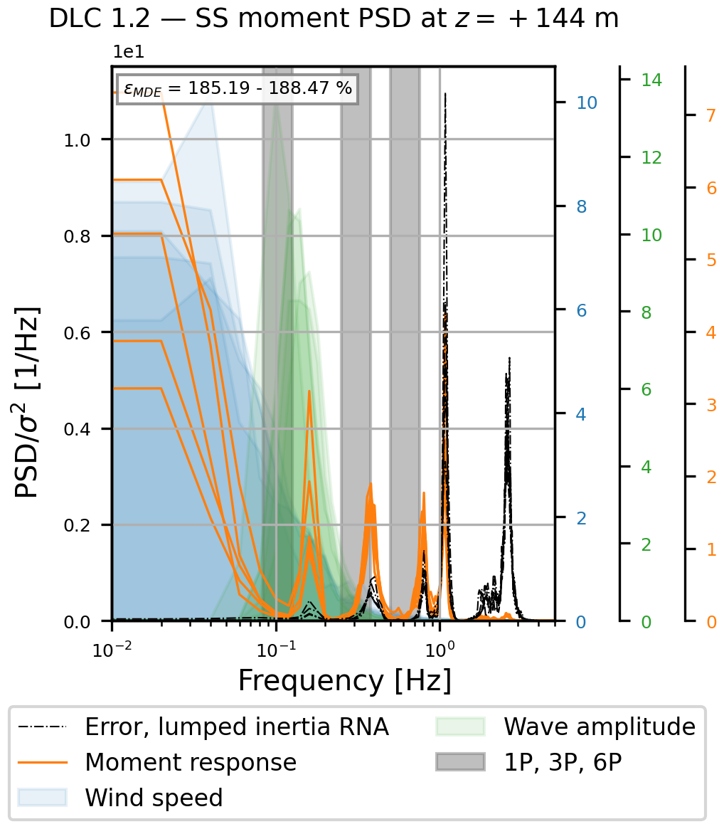
Figure 16 Normalised PSDs representing the MDE performance for the SS moment at the 144 m elevation for five selected moment histories in DLC 1.2. The corresponding selected moment histories are presented in Fig. C2. The PSDs include (1) the MDE error for the lumped-inertia RNA model (black), (2) the 10 min section moment time series (orange), (3) the wind speed in the FA direction (light blue), and (4) the wave amplitude (green). The grey bands indicate the 1P, 3P, and 6P excitation frequencies.

Figures 15 and particularly 16 show that tower top MDE errors observed for DLC 1.2 in Figs. 13 and 14 are highly related to the second and partly third tower bending modes (at ≈1.1 Hz and 2.4–2.6 Hz) in both the FA and the SS directions. As shown by Reinhardt et al. (2024), these mode shapes are highly sensitive to the inclusion of flexible blades in the rotor model, whereby the error might be improved by the inclusion of a flexible rotor in the RNA model. Furthermore, Fig. 14 shows that the MDE error increases proportionally with wind speed for DLCs 1.2 and 2.4 in both the FA (top) and the SS (bottom) directions. This may be explained by blade flexibility, which is dependent on the rotor speed due to e.g. gyroscopic stiffening and blade pitch. Consequently, the MDE error will, to some extent, depend on the wind speed. This dependency may also arise from varying forced excitation from wind and waves, as well as the excitation of different modes due to the varying turbulence, as these effects may not be equally well represented by the MDE.

5.3.2 DLC 6.4: MDE error at tower top

The present section considers the MDE error (ε_MDE) at the tower top elevation (Figs. 13 and 14) for DLC 6.4 (idle rotor). Figure 13 shows that the MDE underestimates the DES in the FA (a) direction, while in the SS (b) direction, the tower top error is considered to be insignificant. However, Fig. 14 shows that the maximum MDE error (ε_MDE) in the FA (top) direction is approximately 15 %, while reaching approximately 13 % in the SS (bottom) direction.

Due to the low DES and small discrepancies observed between MDE and HAWC2 DES for DLC 6.4 in Fig. 13b, the MDE error is not considered further for the SS direction. However, the moment histories from DLC 6.4, corresponding to the five largest MDE errors at an elevation of 144 m in the FA direction, have been selected for further analysis. These are presented in Fig. C3, and the PSDs representing the moment response are presented in Fig. 17, following the approach as in Sect. 5.3.1.

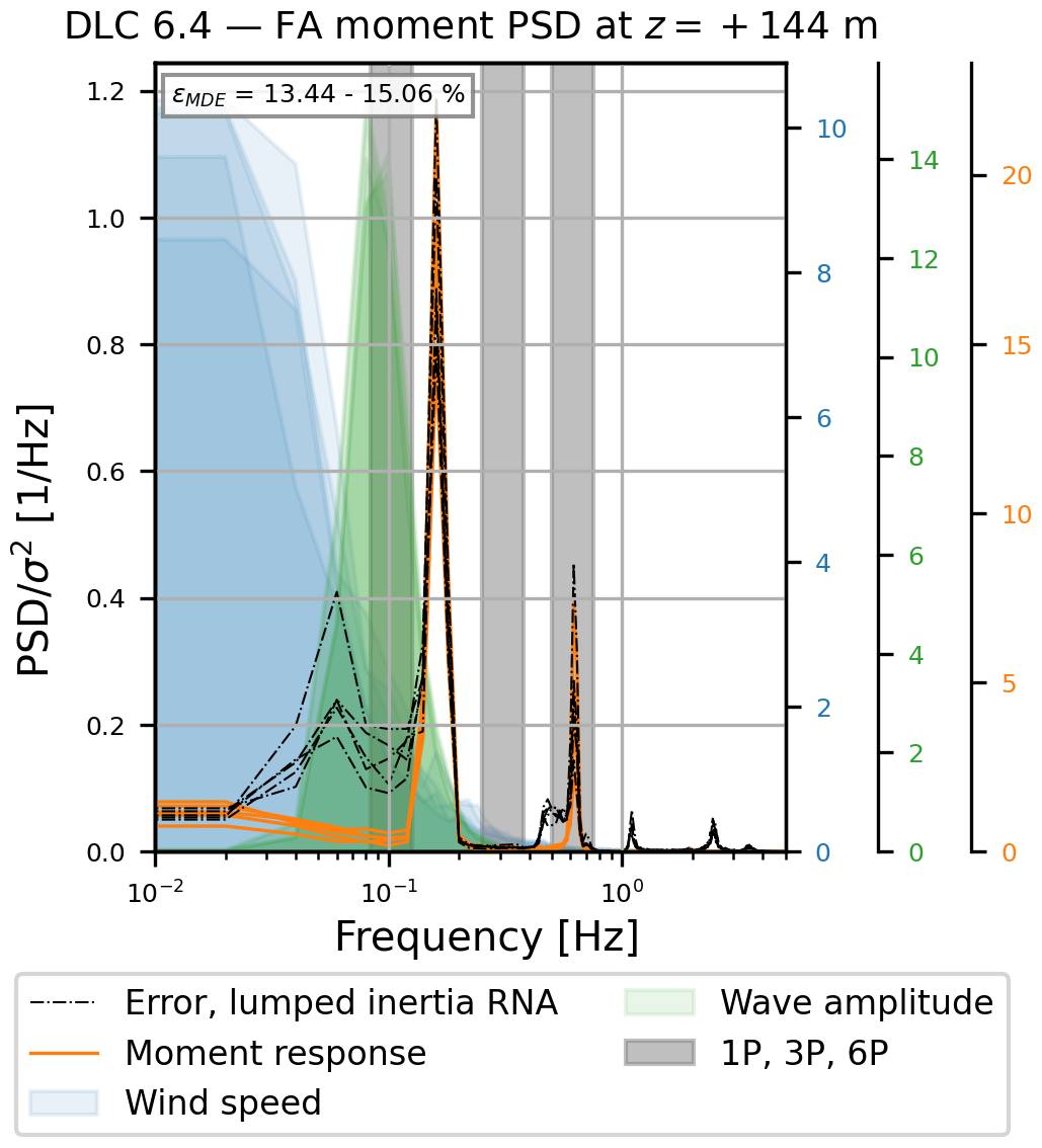
Figure 17 Normalised PSDs representing the MDE performance for the FA moment at the 144 m elevation for five selected moment histories in DLC 6.4. The corresponding selected moment histories are presented in Fig. C3. The PSDs include (1) the MDE error for the lumped-inertia RNA model (black), (2) the 10 min section moment time series (orange), (3) the wind speed in the FA direction (light blue), and (4) the wave amplitude (green). The grey bands indicate the 1P, 3P, and 6P excitation frequencies.

Figure 17 shows that the dominating frequency for the MDE error (ε_MDE) for the moment history at the tower top for DLC 6.4 coincides with the natural frequency of the first tower bending modes at approximately 0.16 Hz. This error may be a result of a discrepancy between the mode shapes extracted from the prediction FE model and the actual mode shapes of the IEA 15 MW RWT. However, since frequency band B₃ utilises mode shapes and Ritz vectors which are not orthogonal to each other, the error may also stem from the matrix Φ_m being ill-conditioned, leading to an erroneous model decomposition for this frequency band. It is therefore relevant to investigate the implications for the MDE results arising from the current lack of independence of the Ritz vectors and mode shapes applied in B₃.

In addition to the MDE error at 0.16 Hz, a pronounced error peak in the MDE error PSD is associated with the natural frequency of the first edgewise blade mode, at approximately 0.64 Hz, where a significant contribution to the moment response is also observed (Fig. 17). This underlines that not only the tower modes but also the rotor modes contribute to the DES, and these must be accurately accounted for by the MDE.

Finally, Fig. 14 shows that the wind speed dependency of ε_MDE is less obvious for DLC 6.4 than for DLC 1.2. This could be attributed to vibrations being governed by the inherent dynamics of the wind turbine (first tower bending modes and the first edgewise blade mode, as shown in Fig. 17 for DLC 6.4), which are not influenced by operational variability (e.g. gyroscopic stiffening and blade pitching) for an idle rotor. However, it is likely because DLC 6.4 is only considered for wind speeds above 25 m s⁻¹.

5.3.3 DLC 7.2: MDE error at tower top

The present section considers the MDE error (ε_MDE) at the tower top elevation (Figs. 13 and 14) for DLC 7.2 (locked rotor). For DLC 7.2, a large variance is observed for the MDE error (ε_MDE) at the tower top, being in the ranges ±25 % in the FA (top) direction and ±20 % in the SS (bottom) direction, respectively. It is somewhat surprising that the large variance in the error ε_MDE for DLC 7.2 in the SS direction, shown in Fig. 14(bottom), results in such small discrepancies in the HAWC2 and MDE DESs, shown in Fig. 13b. However, it underlines that the long-term MDE prediction is mostly sensitive to biased errors.

As for DLC 1.2, five FA and five SS moment histories from DLC 7.2 have been further analysed to contextualise the behaviour observed in Figs. 13 and 14. However, the DLC 7.2 moment histories have been selected based on their absolute MDE rather than their relative MDE error (ε_MDE), as previously mentioned. The selected moment histories for DLC 7.2 are presented in Figs. C4 and C5, and the PSDs representing the moment responses are presented in Figs. 18 and 19, following the approach as in Sect. 5.3.1.

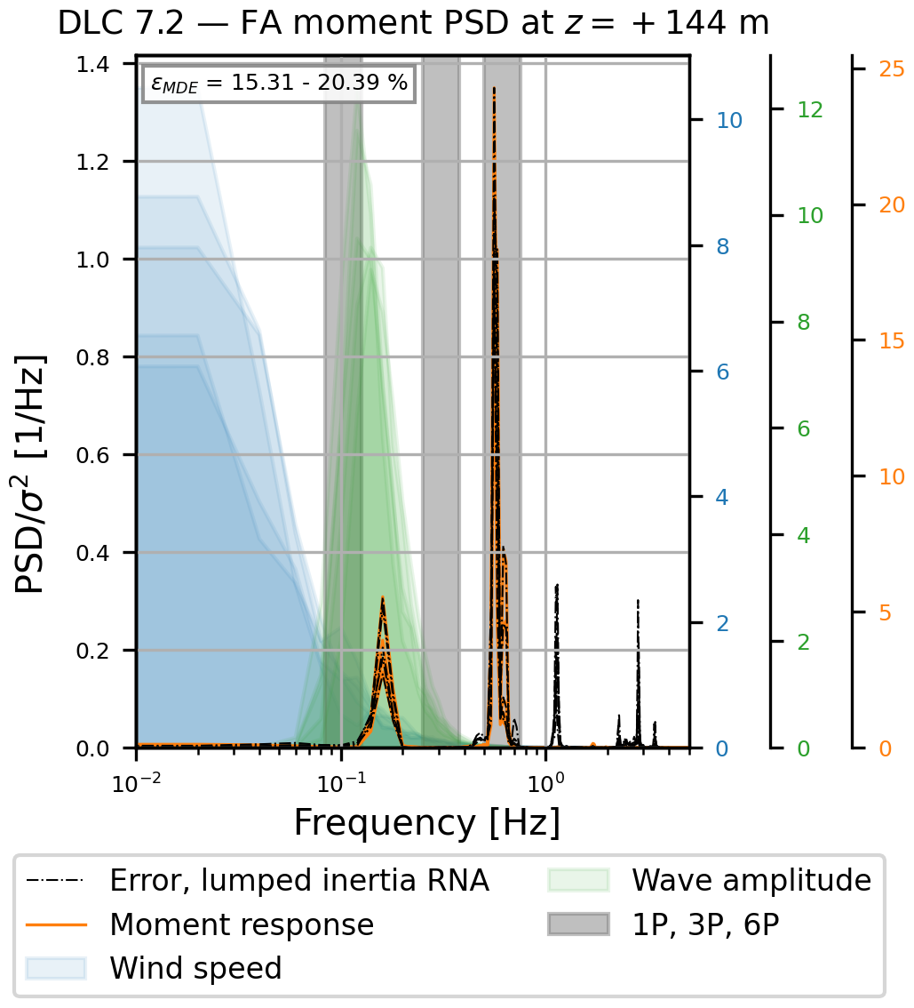
Figure 18 Normalised PSDs representing the MDE performance for the FA moment at the 144 m elevation for five selected moment histories in DLC 7.2. The corresponding selected moment histories are presented in Fig. C4. The PSDs include (1) the MDE error for the lumped-inertia RNA model (black), (2) the 10 min section moment time series (orange), (3) the wind speed in the FA direction (light blue), and (4) the wave amplitude (green). The grey bands indicate the 1P, 3P, and 6P excitation frequencies.

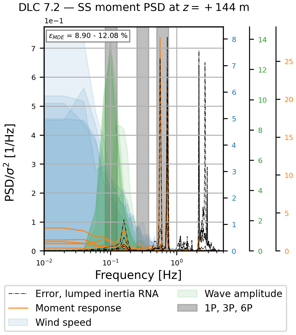
Figure 19 Normalised PSDs representing the MDE performance for the SS moment at the 144 m elevation for five selected moment histories in DLC 7.2. The corresponding selected moment histories are presented in Fig. C5. The PSDs include (1) the MDE error for the lumped-inertia RNA model (black), (2) the 10 min section moment time series (orange), (3) the wind speed in the FA direction (light blue), and (4) the wave amplitude (green). The grey bands indicate the 1P, 3P, and 6P excitation frequencies.

In contrast to the idle-rotor configuration (DLC 6.4), the locked-rotor configuration (DLC 7.2) enables excitation of both the flapwise and the edgewise blade modes. Thus, the wind turbine is susceptible to excitation of different rotor modes by different wind fields in the locked configuration. This is shown in Figs. 18 and 19, where the PSD of the moment response exhibits significant peaks at different frequencies near the natural frequencies of the first flapwise and edgewise blade modes (at ≈0.56 and 0.64 Hz). Figures 18 and 19 also demonstrate that significant contributions to the MDE error arise from the rotor modes at these frequencies. This indicates the need to include a rotor mode in the multi-band MDE for this DLC, which cannot be achieved using a lumped-inertia RNA model.

5.3.4 MDE error at ±15 m MSL

The present section considers the MDE error (ε_MDE) present for all of the considered DLCs at ±15 m around MSL. Figure 14 shows that the MDE generally underestimates the moment DES in the region around MSL, with the maximum MDE error for the individual DLCs being approximately in the range −3 % to −6 %.

To explain the underlying reason for MDE error in this region, five moment histories, corresponding to the five largest MDE errors at an elevation of 0 m for DLC 1.2 in the FA and SS directions and DLC 6.4 in the FA direction, respectively, have been selected for further analysis. Figures C6, C7, and C8 present segments of the moment histories, while Figs. 20, 21, and 22 provide an overview of the moment response, following the approach from Sect. 5.3.1.

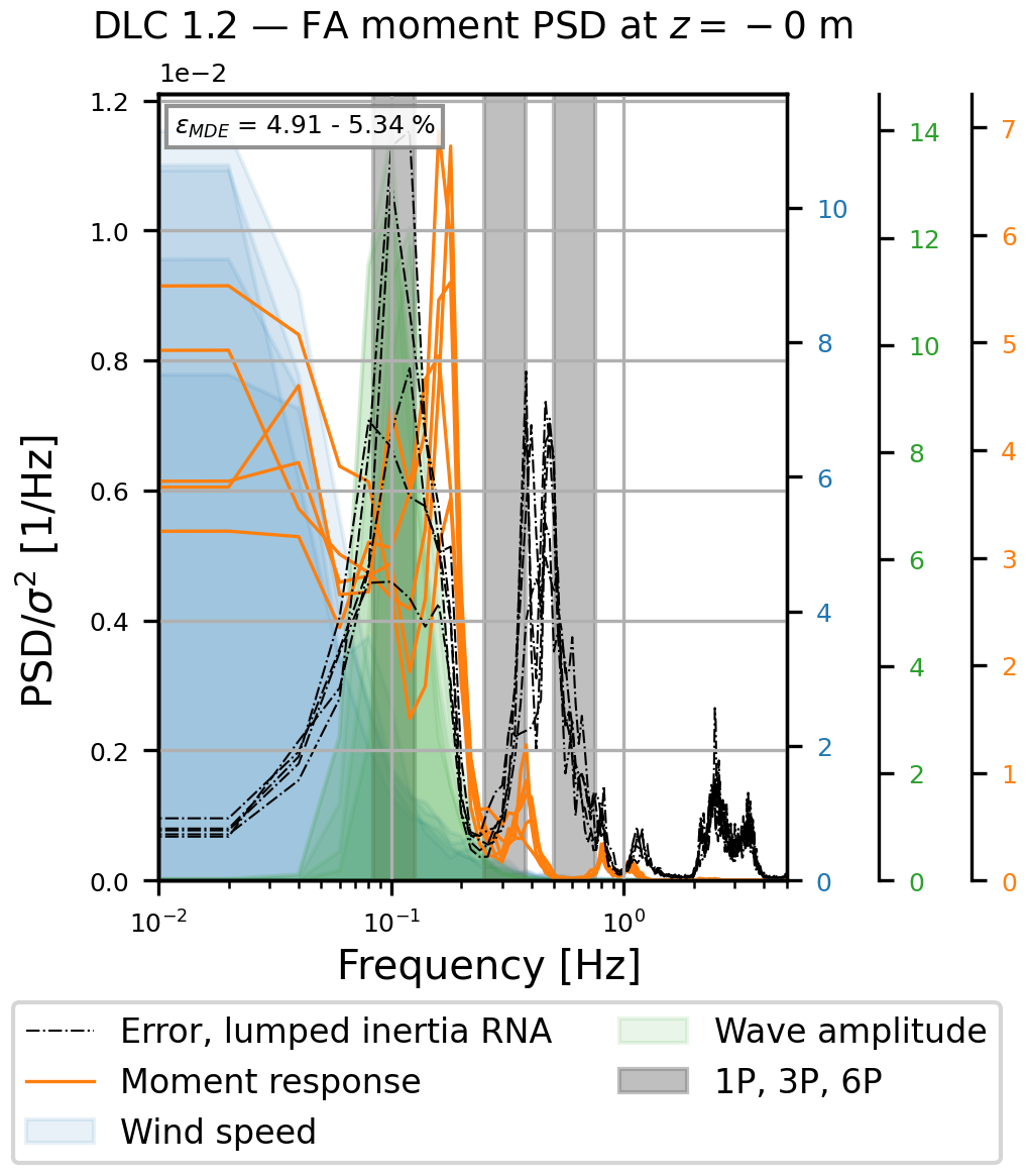
Figure 20 Normalised PSDs representing the MDE performance for the FA moment at the 0 m elevation for five selected moment histories in DLC 1.2. The corresponding selected moment histories are presented in Fig. C6. The PSDs include (1) the MDE error for the lumped-inertia RNA model (black), (2) the 10 min section moment time series (orange), (3) the wind speed in the FA direction (light blue), and (4) the wave amplitude (green). The grey bands indicate the 1P, 3P, and 6P excitation frequencies.

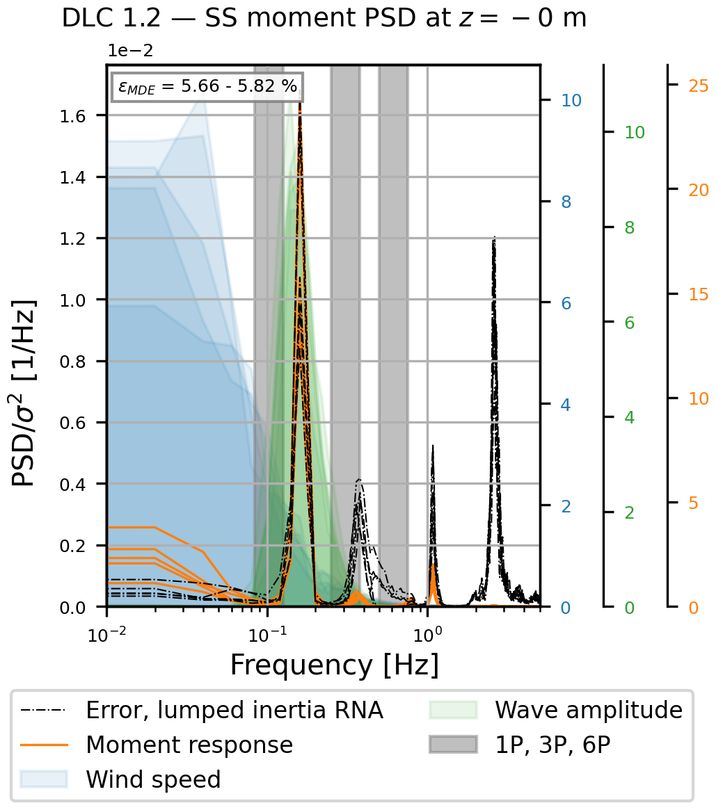
Figure 21 Normalised PSDs representing the MDE performance for the SS moment at the 0 m elevation for five selected moment histories in DLC 1.2. The corresponding selected moment histories are presented in Fig. C7. The PSDs include (1) the MDE error for the lumped-inertia RNA model (black), (2) the 10 min section moment time series (orange), (3) the wind speed in the FA direction (light blue), and (4) the wave amplitude (green). The grey bands indicate the 1P, 3P, and 6P excitation frequencies.

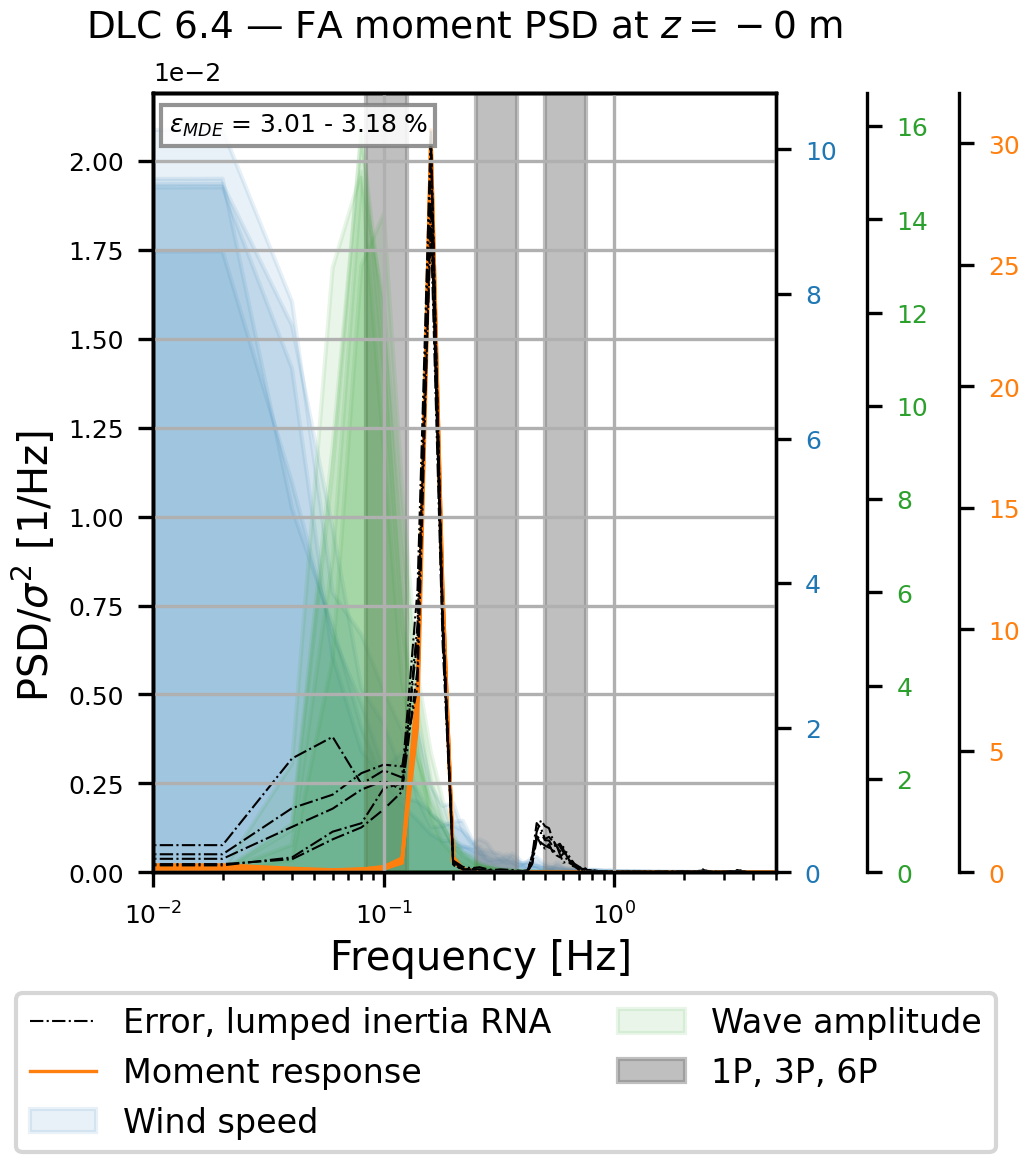
Figure 22 Normalised PSDs representing the MDE performance for the FA moment at the elevation 0 m for five selected moment histories in DLC 6.4. The corresponding selected moment histories are presented in Fig. C8. The PSDs include (1) the MDE error for the lumped-inertia RNA model (black), (2) the 10 min section moment time series (orange), (3) the wind speed in the FA direction (light blue), and (4) the wave amplitude (green). The grey bands indicate the 1P, 3P, and 6P excitation frequencies.

Figure 20 shows that the main contribution to the MDE error in the FA direction at MSL coincides with the natural frequencies for the waves for DLC 1.2. This behaviour can be attributed to the MDE errors arising from using a wave model that is too simple. The wave load Ritz vectors do not account for wave height fluctuations or the dynamic interchange between drag and inertia forces. Furthermore, the wave load is applied to the monopile between the mud line and MSL, thus ignoring the change in loading area during the transition from wave trough to crest. In conclusion, the wave load Ritz vector is unable to capture the full complexity of the actual wave load in the IEA 15 MW RWT HAWC2 model.

In the SS direction, where aerodynamic damping is significantly lower, the response is governed by structural dynamics rather than wave loads. Consequently, the error PSD coincides with the first three SS tower bending modes, approximately 0.16, 1.1, and 2.6 Hz. In this direction, the waves are less influential, as they are generally more aligned with the FA direction. Furthermore, due to the low aerodynamic damping in the SS direction compared to the FA direction, the response is mainly dominated by the inherent structural dynamics of the IEA 15 MW RWT, and thus, the relative contribution from the waves to the moment response is small. This is also underlined by the MDE error observed in the FA direction for DLC 6.4 (Fig. 22), which is dominated by the first FA tower bending mode, resulting in the forced excitation being of small significance.

As the error observed in Figs. 21 and 22 cannot be explained by the wave load Ritz vector, the reason for the MDE error for these moment histories is more likely related to discrepancies between the mode shapes of the FE prediction model and the actual mode shapes of the IEA 15 MW RWT. However, the MDE error might also arise from the lack of independence of the mode shapes and Ritz vectors in frequency band B₃, as discussed previously.

5.4 Summary

When combining the conclusions from the above discussion, it is assessed that the MDE used in the present work generally performs well, except at the tower top, where it performs inconsistently across the different considered DLCs. Furthermore, in the ±15 m range around MSL, the MDE consistently underestimates the DES, resulting in an error of up to 6 %. This may be improved by further enhancing the MDE as described below, although, in practice, a 5 %–6 % error level may be overshadowed by other uncertainties. Hereby, the main challenges associated with the present use of MDE the following:

• capturing the local effects of the flexible and dynamic response of the rotor and blades

• including the effects from rotor flexibility and operation in the tower mode shapes used in the MDE

• including the relevant rotor modes for the standstill DLCs (6.4 and 7.2)

• including wind speed variability and time dependency of the waves in the MDE

• ensuring independent mode shapes and Ritz vectors while representing various forced excitations and excited structural modes in the same frequency bands.

Some of the errors observed in the present section may also be related to the chosen sensor locations and the associated MDE configuration presented in Sect. 5.1. However, as noise is not included in the present analysis, the noise-to-signal ratio is not an issue, whereby a non-optimal sensor location would have less impact in the present comparison.

6 Conclusions

This paper presents an overview of the dataset available in Pedersen et al. (2025), containing response simulations covering the fatigue limit state (FLS) design life of the IEA Wind 15 MW offshore reference wind turbine with a monopile foundation (IEA 15 MW RWT) version 1.1.6.

The paper explores how diverse operational and environmental scenarios impact the damage equivalent loads (DELs) calculated from the fore–aft (FA) and side–side (SS) section moment histories at the tower base, after which the relative lifetime damage for the individual FLS design load cases (DLCs), described in IEC 61400-3-1:2019 (IEC, 2019b), is calculated at all nodes in the support structure of the IEA 15 MW RWT. It has been found that the DLCs representing power production in normal conditions (DLC 1.2), a parked turbine with an idle rotor in normal conditions (DLC 6.4), and a fault of a locked rotor in normal conditions (DLC 7.2) govern the lifetime damage of the support structure. The high contribution from DLC 1.2 occurs because of its long duration (90 % of the design life) and the excitation at the tower top caused by 3P effects, while the contribution of DLCs 6.4 and 7.2 is large because of their high DELs associated with low aerodynamic damping. The damage associated with start-up and particularly shut-down in normal conditions (DLCs 3.1 and 4.1) might be significantly underestimated in the present paper, as the durations specified by IEC (2019b) for these DLCs do not necessarily reflect a real operation scenario, where start-up and shut-down can occur for many reasons, including curtailment.

The paper gives an overview of multi-band modal decomposition and expansion (MDE) and a methodology for expressing the estimated response in sectional forces, after which it presents the finite-element (FE) model used to calculate the Ritz vectors and mode shapes used to perform MDE. It explains the configuration used to perform MDE for the estimation of section moment time histories in the support structure of the IEA 15 MW RWT, which is based on rotation and displacement data from six HAWC2 sensors located at three elevations in the RWT tower (in both the FA and the SS directions), and includes both the quasi-static and the dynamic part of the frequency response.

The present work utilises MDE to estimate section moment histories in all nodes of the support structure of the IEA 15 MW RWT across different operational and environmental regimes represented in the data from Pedersen et al. (2025). Based on the moment histories, the combined DELs of the individual DLCs are calculated along with the combined DESs for the individual DLCs and the DESs from the individual HAWC2 simulations. The MDE generally performs well in estimating the combined DELs and DESs for the individual DLCs. However, its accuracy strongly depends on the elevation considered on the IEA 15 MW RWT support structure. Thus, notable errors occur around the tower top, specifically from 120–144 m above mean sea level (MSL) and at ±15 m MSL. The error magnitude is also influenced by the operational and environmental conditions of the OWT, as highlighted by the dependency of the MDE error on the DLC considered. This is directly related to the external forces and structural modes dominant in each DLC. This is emphasised by the errors at the tower top, which are closely linked to the second and third tower bending modes in DLC 1.2 and to various rotor modes in DLC 7.2. As these modes are sensitive to rotor flexibility, the MDE performance in the tower top region may be improved by including rotor flexibility in the rotor nacelle assembly (RNA) model rather than using a lumped-inertia RNA model. Furthermore, the MDE errors at MSL may be attributed to limitations of the Ritz vector used to represent the wave loads for DLC 1.2 in the FA direction, whereas the error may stem from erroneous tower mode shapes in the SS direction. It is also suggested that the linear dependency between the mode shapes and Ritz vectors used in the MDE in the low-frequency band B₃ may result in MDE errors.

The relative MDE errors for the DESs of the individual HAWC2 simulations ε_MDE are predominantly in the range of ±5 %, thus confirming that the MDE performs well in general. These MDE errors also underline that the MDE performs poorly around the tower top, where errors of up to 188 % are observed. Finally, the MDE errors show a wind speed dependency. It is concluded that the wind speed dependency of the MDE error is caused by environmental and operational variability of the rotor, which is not captured by the MDE assuming a linear and time-invariant response. Additionally, the lumped-inertia RNA model and the wave load Ritz vector, which do not incorporate wind speed variability and the time-dependent nature of waves, likely contribute further to the observed wind speed dependency of the MDE error.

In future work, the authors suggest investigating the effects of including a flexible rotor in the FE model used to obtain the mode shapes used in the MDE. The knowledge obtained from the present work will serve as a basis for updating the RNA model to include blade flexibility and, subsequently, to include operational and environmental variability in RNA modelling, e.g. by using individual RNA models for various wind speeds. The authors also plan to implement a wave load model that accounts for the waves' variation with wind speed. Finally, it would be vital to investigate the MDE accuracy of a reduced number of physical sensors, e.g. from existing monitoring systems, not specifically designed for virtual sensing purposes.

Appendix A: Database description

The present appendix briefly describes the IEA 15 MW RWT, as well as the modelling assumptions and design load cases (DLCs) considered in Pedersen et al. (2025).

A1 IEA Wind 15 MW offshore reference wind turbine

The IEA 15 MW RWT is a monopile-founded offshore wind turbine with a rated power of 15 MW and a cut-in, rated, and cut-out wind speed of V_in = 3 m s⁻¹, V_r = 10.69 m s⁻¹, and V_out = 25 m s⁻¹, respectively. The support structure consists of a 75 m monopile with an embedment depth of 45 m, a 15 m transition piece, and a 129.4 m tower; see Fig. 1. The design of the support structure has been derived from the ultimate limit state (ULS) and modal analysis following a soft–stiff approach (Gaertner et al., 2020a), thus locating the natural frequency of approximately 0.17 Hz for the first-order tower bending modes between the 1P and 3P rotor frequencies. The design of the IEA 15 MW RWT is available from the GitHub repository in Gaertner et al. (2023).

A2 Modelling

As previously stated, the database in Pedersen et al. (2025) comprises synthetic wind turbine response data obtained by HAWC2 simulations, whereby it inherits the limitations and assumptions associated with HAWC2. HAWC2 calculates the aerodynamic loads based on blade element momentum (BEM) theory. The implementation of BEM theory in HAWC2 has been extended to account e.g. for dynamic inflow, dynamic stall, and the rotor's yaw and tilt (Larsen and Hansen, 2021). In the present work, the turbulent wind field is modelled using the Mann turbulence generator, which is directly linked with HAWC2. The tower shadow effect is accounted for using a potential flow model, and the wind shear is implemented using the standard power law expression

$$\begin{array}{}\text{(A1)}& V\left(z\right)=V\left(z_{\mathrm{r}}\right){\left({\displaystyle \frac{z}{z_{\mathrm{r}}}}\right)}^{\mathit{\alpha }},\end{array}$$

where V(z) is the wind speed across the elevation z above mean sea level (MSL), z_r is the reference elevation at which the wind speed V(z_r) is known (in this case at hub height), and α=0.08 from the metocean assessment in DHI (2023a).

The structural modelling in HAWC2 is based on a multi-body formulation, where each body is an assembly of Timoschenko beam elements. Thus, the formulation for the structural members accounts for large deflections and rotations, geometrical non-linearities, and shear deformations (Larsen and Hansen, 2021). The soil model implemented in the model for simulations performed by Pedersen et al. (2025) utilise the lateral linear soil springs presented in Table A1. In HAWC2, the hydrodynamic forces acting on the monopile are calculated using Morison's formula. The present work ignores the current when calculating hydrodynamic forces, and the water kinematics are calculated based on the irregular Pierson–Moskowitz wave spectrum, utilising the significant wind-speed-dependent wave height and the wave period from the metocean assessment in DHI (2023c).

Table A1 Lateral spring stiffness of soil in node n of the embedded part of the monopile (presented in Fig. 6) as a result of the z coordinate presented in Fig. 1. Defined in Appendix B.2 in Gaertner et al. (2020a) and used by Pedersen et al. (2025).

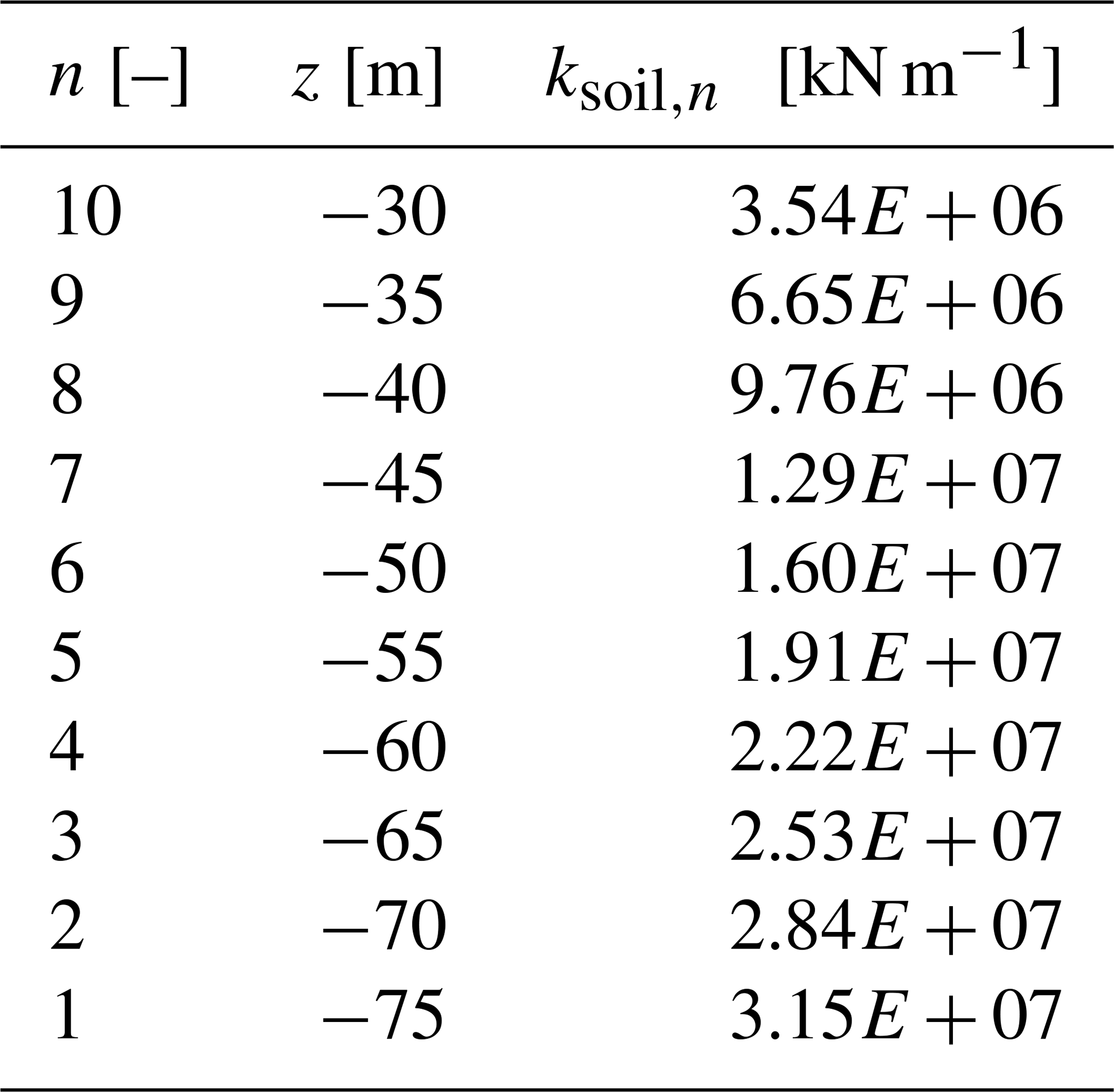
A3 Load cases

The design load cases (DLCs) for the fatigue limit state (FLS) of bottom-fixed OWTs are described in IEC 61400-3-1:2019 (IEC, 2019b). In Pedersen et al. (2025), the implementation of the DLCs follows Natarajan et al. (2016), with the input values used for the HAWC2 simulations presented in Table A2. The number of simulations in Table A2 is a result of the operational and environmental variability needed to capture the individual load cases, e.g. DLC 1.2 considers 11 different wind speeds at three different yaw errors, wind–wave misalignments, and mean water levels (MWLs). Finally, six seeds are used to secure numerical robustness for the simulation of both turbulence and irregular waves. In total, this gives $\mathrm{11}\times \mathrm{3}\times \mathrm{3}\times \mathrm{3}\times \mathrm{6}=\mathrm{1782}$ simulations for DLC 1.2. According to DHI (2023b), the tidal effects at the chosen site are weak, and thus only the simulations where the MWL is equal to the MSL are considered, thereby discarding simulations where the MWL is at either the lowest (LAT) or the highest (HAT) astronomical tide in the analysis conducted for the present paper.

To evaluate the lifetime damage contribution from the individual HAWC2 simulations, their representative durations are calculated based on the joint probability of the DLC occurrence and the environmental parameters: wind speed, yaw error, and wind–wave misalignment. An overview of the input for the duration of the individual simulations is presented in Table A3. The duration of the individual DLCs is based on the recommendations in Sect. 7 of IEC (2019b). The application of these recommendations in the present work is presented below.

• DLC 1.2. It is expected that the wind turbine will be available for operation under normal conditions for 90 % of its 20-year lifetime. In the present work, this is interpreted as DLC 1.2 occurring 90 % of the time when the wind speed falls within the cut-in and cut-out wind speed (V_in = 3 m s⁻¹ and V_out = 25 m s⁻¹).

• DLC 2.4. For operation during the occurrence of fault or loss to the electrical network, IEC (2019b) suggests that the duration may be applied as follows: 10 shut-downs per year for an overspeed event, 24 h per year of operation for events with yaw error, 24 h per year of operation for events with pitch error, and 20 times per year for loss of electrical network connection. In Pedersen et al. (2025), only the fault “operation for events with yaw error” is modelled. To account for the damage occurring during the remaining fault conditions specified for DLC 2.4, the duration is adjusted to 50 h yr⁻¹ of operation (0.57 % of the time the wind speed falls within V_in and V_out) in the present work.

• DLCs 3.1 and 4.1. IEC (2019b) states that start-up/shut-down in normal conditions (DLCs 3.1/4.1) can be expected to occur 1100 times annually: 1000 times at the cut-in wind speed, 50 times at the rated wind speed, and 50 times at the cut-out wind speed (0.35 % of the total life for DLCs 3.1 and 4.1).

• DLC 6.4. In the present analysis, DLC 6.4 is considered to occur only when the wind speed at the hub exceeds the cut-out wind speed V_out=25 m s⁻¹. As this DLC is the only one expected to occur for wind speeds above V_out, the duration of DLC 6.4 is assumed to be the total duration the hub wind speed exceeds the cut-out wind speed.

• DLC 7.2. As IEC (2019b) does not specify a duration for DLC 7.2, this work defines its duration as the time not accounted for by previous DLCs within the operational wind speed range from V_in to V_out, which is 8.7 %.

Table A2 Overview of DLCs from IEC (2019b) considered in Pedersen et al. (2025).

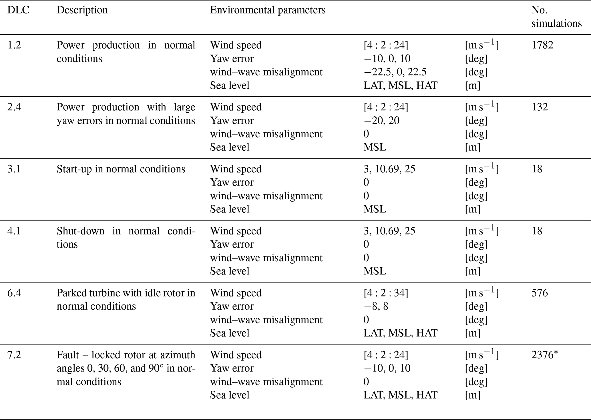
^* 208 simulations of the simulations for DLC 7.2 failed to converge and are disregarded in further work.

Table A3 Input for joint probability used for calculating the expected lifetime duration for the individual time series available in Pedersen et al. (2025).

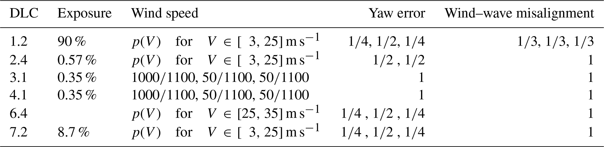
The wind speed's probability density is assumed to follow the Weibull distribution:

$$\begin{array}{}\text{(A2)}& p\left(V\right)={\displaystyle \frac{k}{A}}{\left({\displaystyle \frac{V}{A}}\right)}^{k-\mathrm{1}}\exp \left(-{\left({\displaystyle \frac{V}{A}}\right)}^k\right),\end{array}$$

with the omnidirectional Weibull parameters k=2.35 and A=9.91 m s⁻¹ given in DHI (2023b) for a mean wind speed ${\overline{V}}_{\mathrm{10}}=\mathrm{8.79}$ m s⁻¹ at 10 m above MSL. These values are corrected for the hub height using a wind shear for the normal wind profile (NWP) presented in Eq. (A1). According to IEC (2019b), only part of the wind speed spectrum is considered, namely $V_{\mathrm{hub}}\in [V_{\mathrm{in}},V_{\mathrm{out}}]$ for DLCs 1.2, 2.4, 3.1, 4.1, and 7.2 and $V_{\mathrm{hub}}\in [V_{\mathrm{out}},\mathrm{0.7}{V}_{\mathrm{ref}}]$ for DLC 6.4. As such, it is assumed that there is no contribution to the fatigue life consumption for $V_{\mathrm{hub}}\notin [V_{\mathrm{in}},\mathrm{0.7}{V}_{\mathrm{ref}}]$, where V_ref = 50 m s⁻¹ is the reference wind speed for wind turbine class 1 (IEC, 2019a).

Although the DLCs described above do not exhaustively represent the scenarios occurring during the actual lifetime of an OWT, they provide an overview of the fatigue-life impact from the most common and governing operating scenarios.

Appendix B: Properties of IEA 15 MW RWT support structure

Table B1 Structural properties of element e in the IEA 15 MW RWT support structure. Including the node coordinates of the end nodes in elements n_e,1 and n_e,2, Young's modulus E, the shear modulus G, the outer radius r, the cross-section area A, the moments of inertia I_xx and I_yy, the polar moment of inertia I_p, and the distributed mass m along the height z.

Appendix C: Moment histories

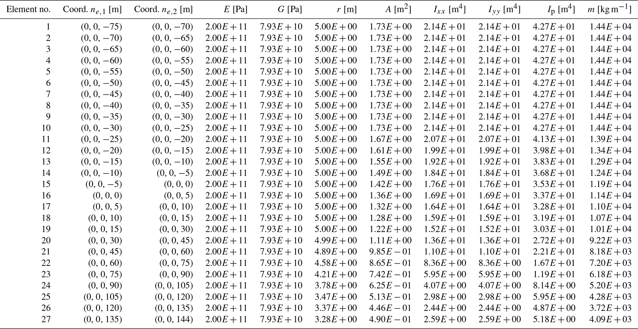
The present appendix presents Figs. C1 to C8, which contain the 20 s segments in the time interval from 390 to 410 s of the moment histories corresponding to the PSDs presented in Sect. 5.3.1 to 5.3.4 and Figs. 15 to 22, respectively. The content of the individual figures are described below:

• Figure C1 shows 20 s segments of the five moment histories corresponding to the five largest relative MDE errors (ε_MDE) occurring in the FA direction at the 144 m elevation for DLC 1.2. The figure provides the HAWC2- and MDE-predicted moment histories, the relative error metric ε_MDE, and the filename for the individual HAWC2 simulations.

• Figure C2 shows 20 s segments of the five moment histories corresponding to the five largest relative MDE errors (ε_MDE) occurring in the SS direction at the 144 m elevation for DLC 1.2. The figure provides the HAWC2- and MDE-predicted moment histories, the relative error metric ε_MDE, and the filename for the individual HAWC2 simulations.

• Figure C3 shows 20 s segments of the five moment histories corresponding to the five largest relative MDE errors (ε_MDE) occurring in the FA direction at the 144 m elevation for DLC 6.4. The figure provides the HAWC2- and MDE-predicted moment histories, the relative error metric ε_MDE, and the filename for the individual HAWC2 simulations.

• Figure C4 shows 20 s segments of the five moment histories corresponding to the five largest absolute MDE errors ($\mathrm{\Delta }{S}_{\mathrm{eq},\mathrm{s},\mathrm{MDE}}-\mathrm{\Delta }{S}_{\mathrm{eq},\mathrm{s},\mathrm{HAWC}\mathrm{2}}$) occurring in the FA direction at the 144 m elevation for DLC 7.2. The figure provides the HAWC2- and MDE-predicted moment histories, the relative error metric ε_MDE, and the filename for the individual HAWC2 simulations.

• Figure C5 shows 20 s segments of the five moment histories corresponding to the five largest absolute MDE errors ($\mathrm{\Delta }{S}_{\mathrm{eq},\mathrm{s},\mathrm{MDE}}-\mathrm{\Delta }{S}_{\mathrm{eq},\mathrm{s},\mathrm{HAWC}\mathrm{2}}$) occurring in the SS direction at the 144 m elevation for DLC 7.2. The figure provides the HAWC2- and MDE-predicted moment histories, the relative error metric ε_MDE, and the filename for the individual HAWC2 simulations.

• Figure C6 shows 20 s segments of the five moment histories corresponding to the five largest absolute MDE errors ($\mathrm{\Delta }{S}_{\mathrm{eq},\mathrm{s},\mathrm{MDE}}-\mathrm{\Delta }{S}_{\mathrm{eq},\mathrm{s},\mathrm{HAWC}\mathrm{2}}$) occurring in the FA direction at the 0 m elevation for DLC 1.2. The figure provides the HAWC2- and MDE-predicted moment histories, the relative error metric ε_MDE, and the filename for the individual HAWC2 simulations.

• Figure C7 shows 20 s segments of the five moment histories corresponding to the five largest absolute MDE errors ($\mathrm{\Delta }{S}_{\mathrm{eq},\mathrm{s},\mathrm{MDE}}-\mathrm{\Delta }{S}_{\mathrm{eq},\mathrm{s},\mathrm{HAWC}\mathrm{2}}$) occurring in the SS direction at the 0 m elevation for DLC 1.2. The figure provides the HAWC2- and MDE-predicted moment histories, the relative error metric ε_MDE, and the filename for the individual HAWC2 simulations.

• Figure C8 shows 20 s segments of the five moment histories corresponding to the five largest absolute MDE errors ($\mathrm{\Delta }{S}_{\mathrm{eq},\mathrm{s},\mathrm{MDE}}-\mathrm{\Delta }{S}_{\mathrm{eq},\mathrm{s},\mathrm{HAWC}\mathrm{2}}$) occurring in the FA direction at the 0 m elevation for DLC 6.4. The figure provides the HAWC2- and MDE-predicted moment histories, the relative error metric ε_MDE, and the filename for the individual HAWC2 simulations.

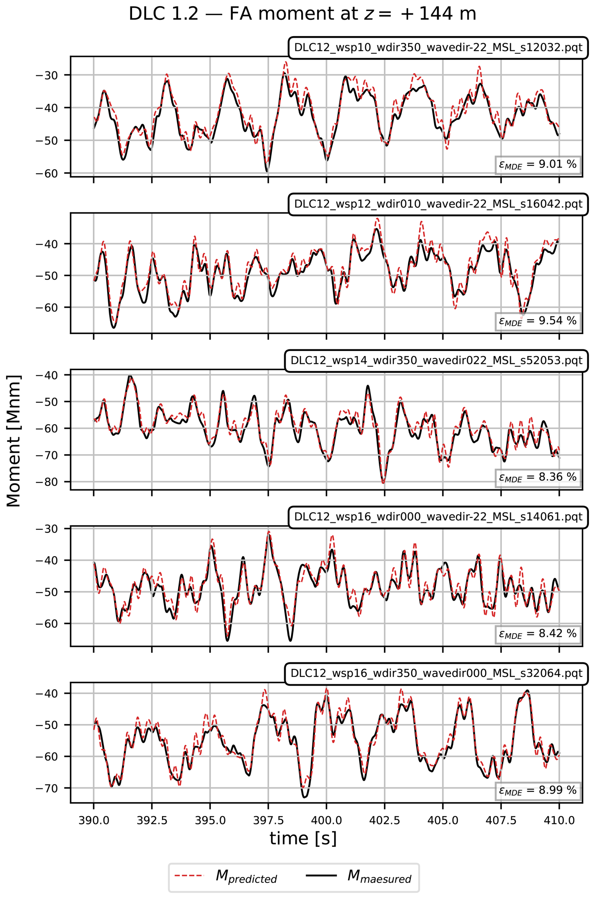
Figure C1 Segments of selected FA moment histories corresponding to the largest relative MDE errors (ε_MDE) at the 144 m above MSL elevation for DLC 1.2. The time series segments include (1) the predicted moment history (red) and (2) the true (or measured) moment history (black).

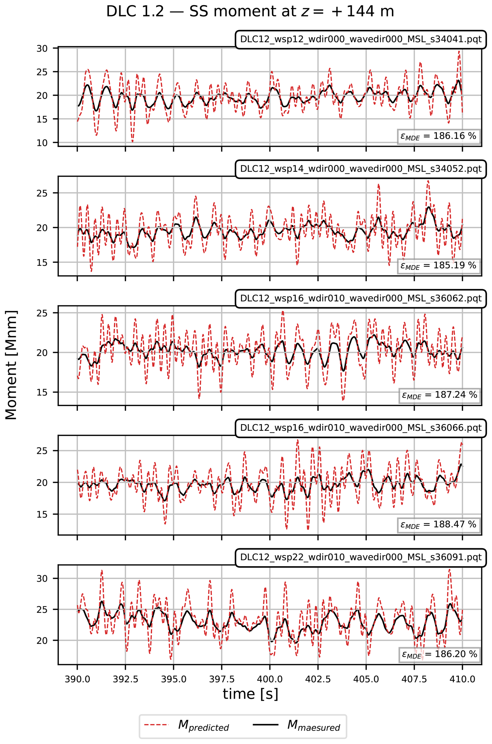
Figure C2 Segments of selected SS moment histories corresponding to the largest relative MDE errors (ε_MDE) at the 144 m above MSL elevation for DLC 1.2. The time series segments include (1) the predicted moment history (red) and (2) the true (or measured) moment history (black).

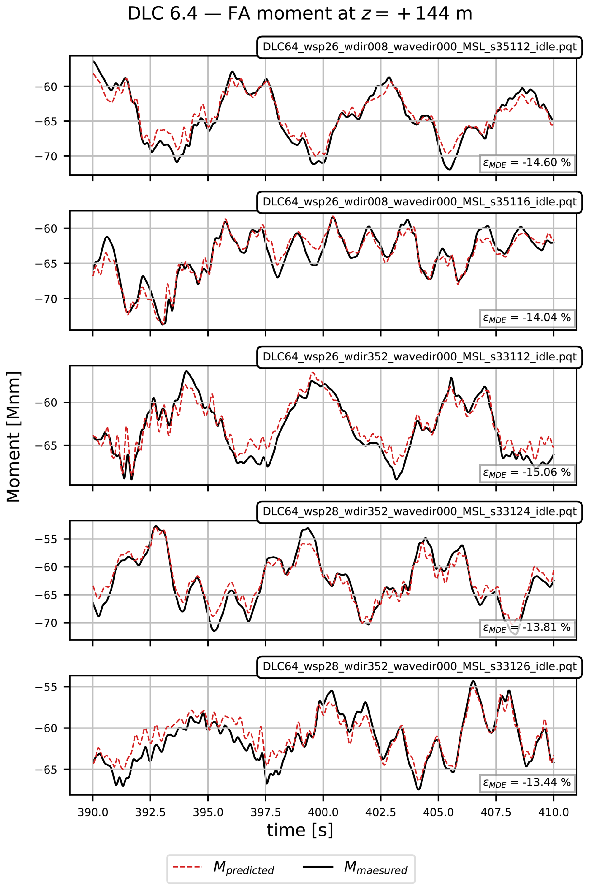
Figure C3 Segments of selected FA moment histories corresponding to the largest relative MDE errors (ε_MDE) at the 144 m elevation above MSL for DLC 6.4. The time series segments include (1) the predicted moment history (red) and (2) the true (or measured) moment history (black).

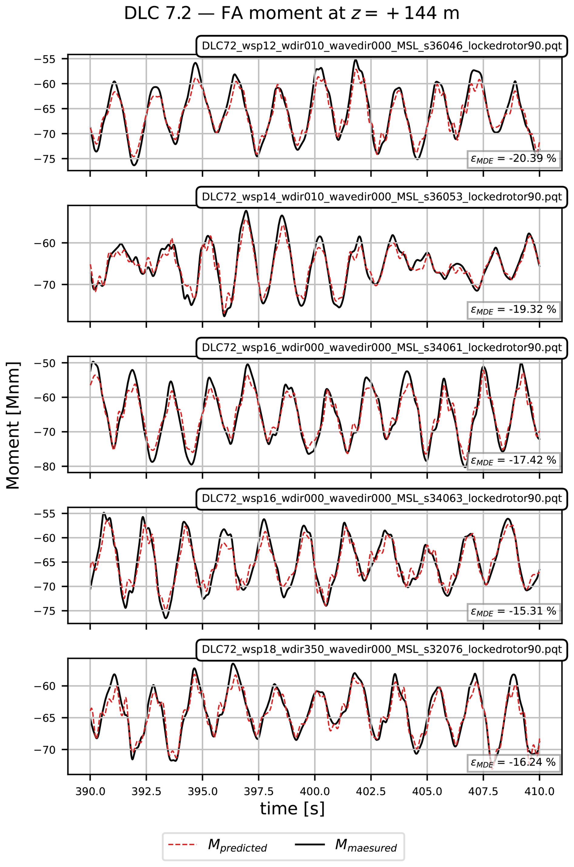
Figure C4 Segments of selected FA moment histories corresponding to the largest absolute MDE errors (ε_MDE) at the 144 m elevation above MSL for DLC 7.2. The time series segments include (1) the predicted moment history (red) and (2) the true (or measured) moment history (black).

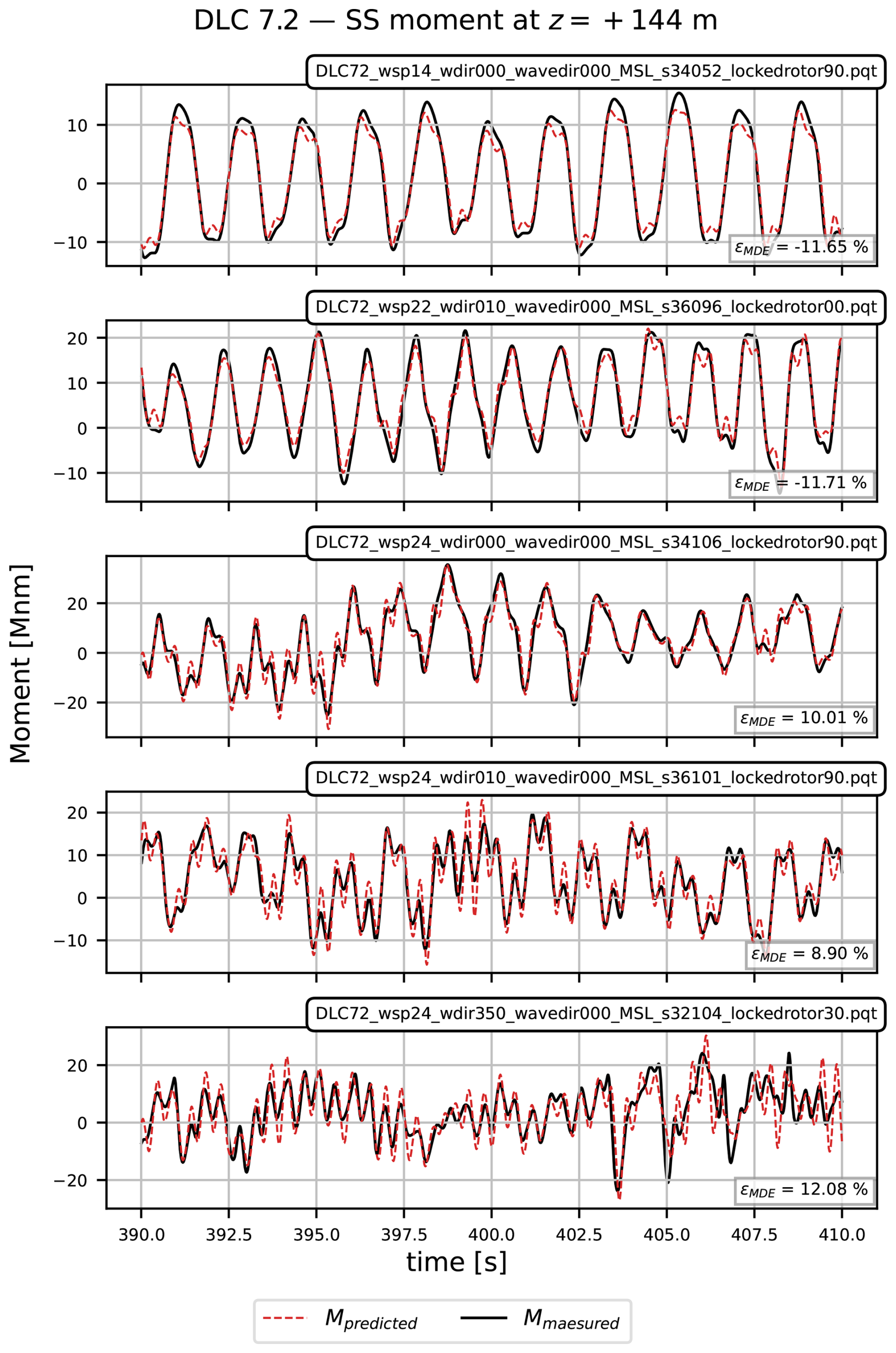
Figure C5 Segments of selected SS moment histories corresponding to the largest absolute MDE errors (ε_MDE) at the 144 m above MSL elevation for DLC 7.2. The time series segments include (1) the predicted moment history (red) and (2) the true (or measured) moment history (black).

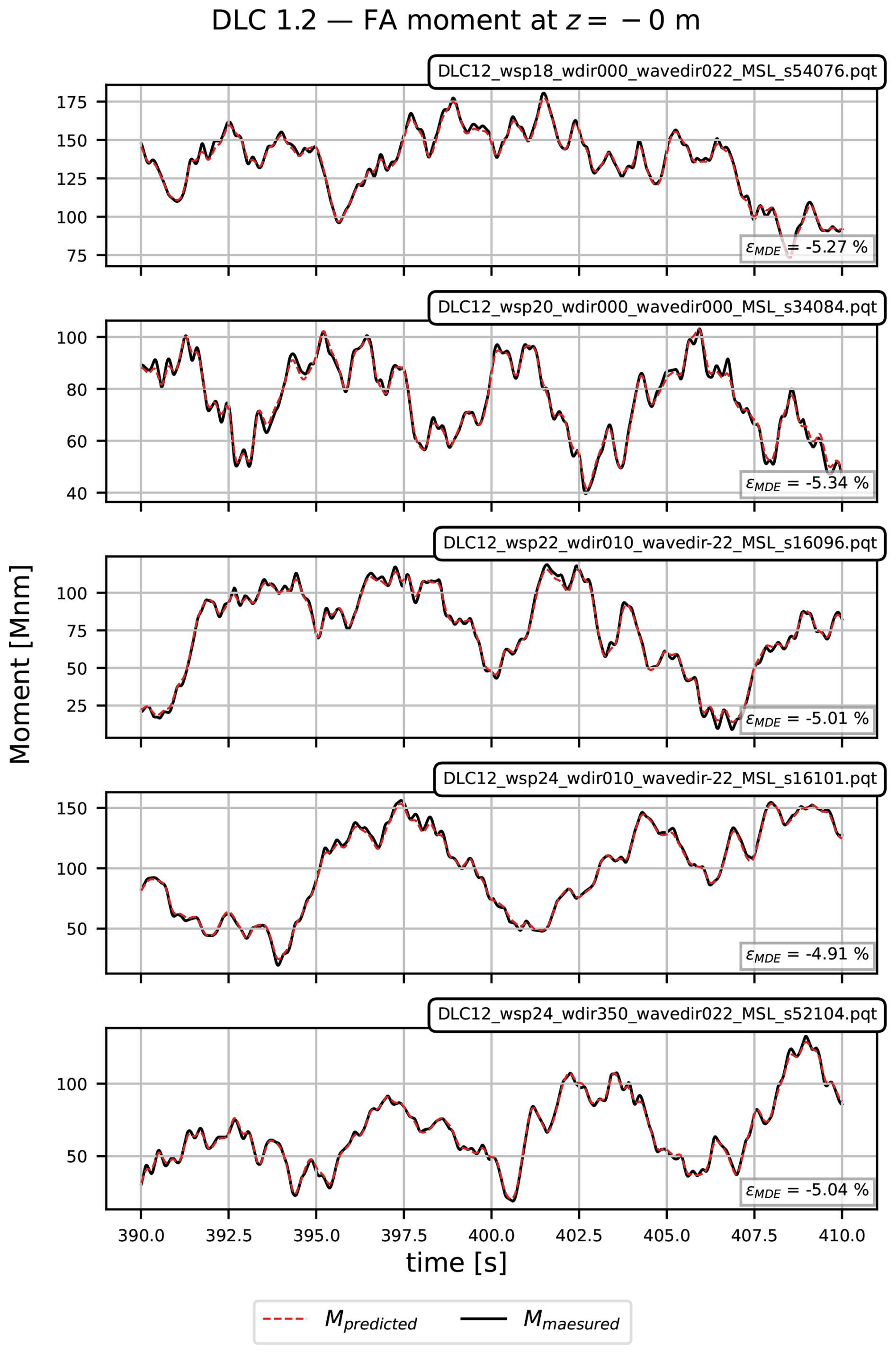
Figure C6 Segments of selected FA moment histories corresponding to the largest relative MDE errors (ε_MDE) at the 0 m above MSL elevation for DLC 1.2. The time series segments include (1) the predicted moment history (red) and (2) the true (or measured) moment history (black).

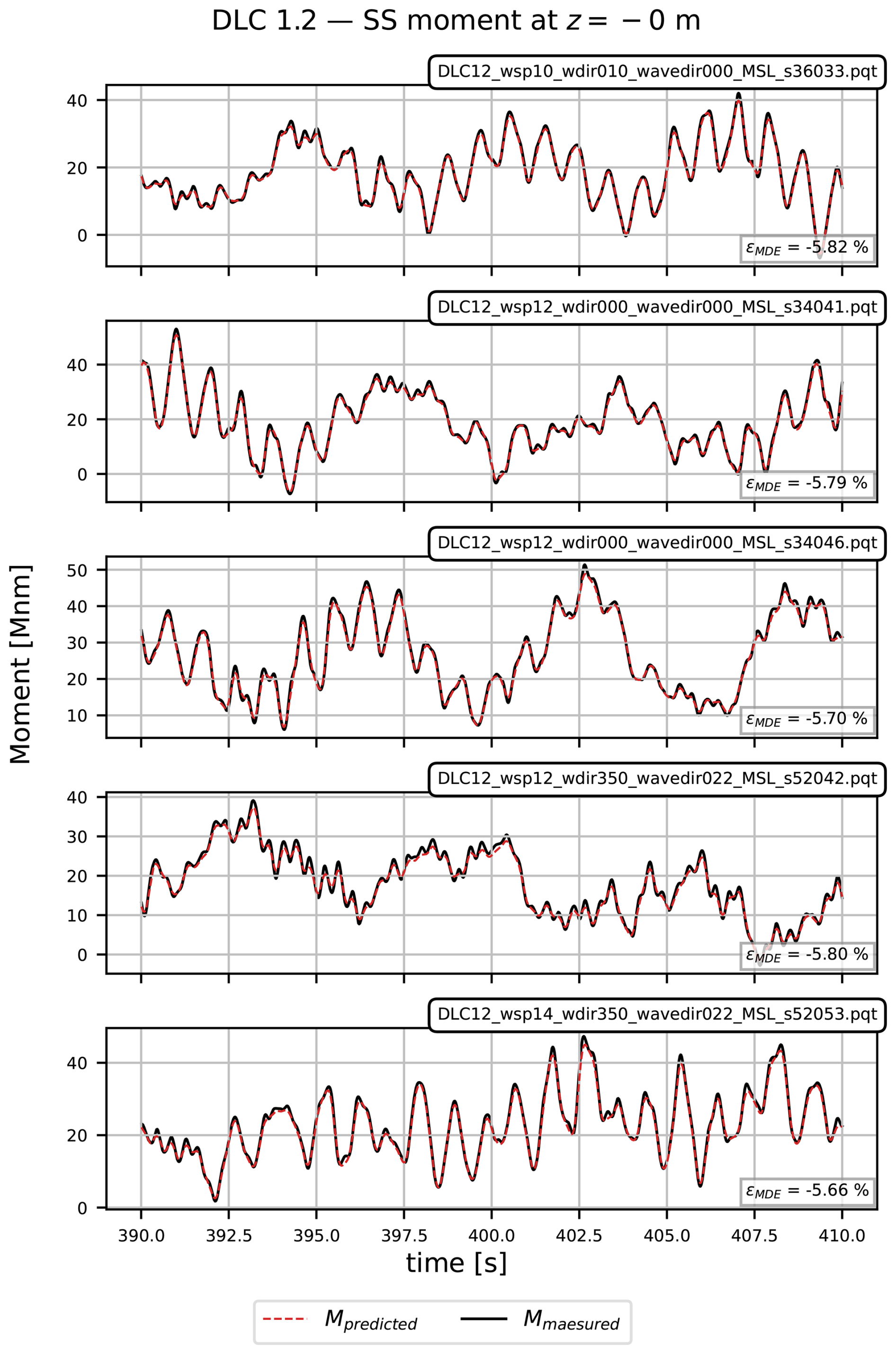
Figure C7 Segments of selected SS moment histories corresponding to the largest relative MDE errors (ε_MDE) at the 0 m above MSL elevation for DLC 1.2. The time series segments include (1) the predicted moment history (red) and (2) the true (or measured) moment history (black).

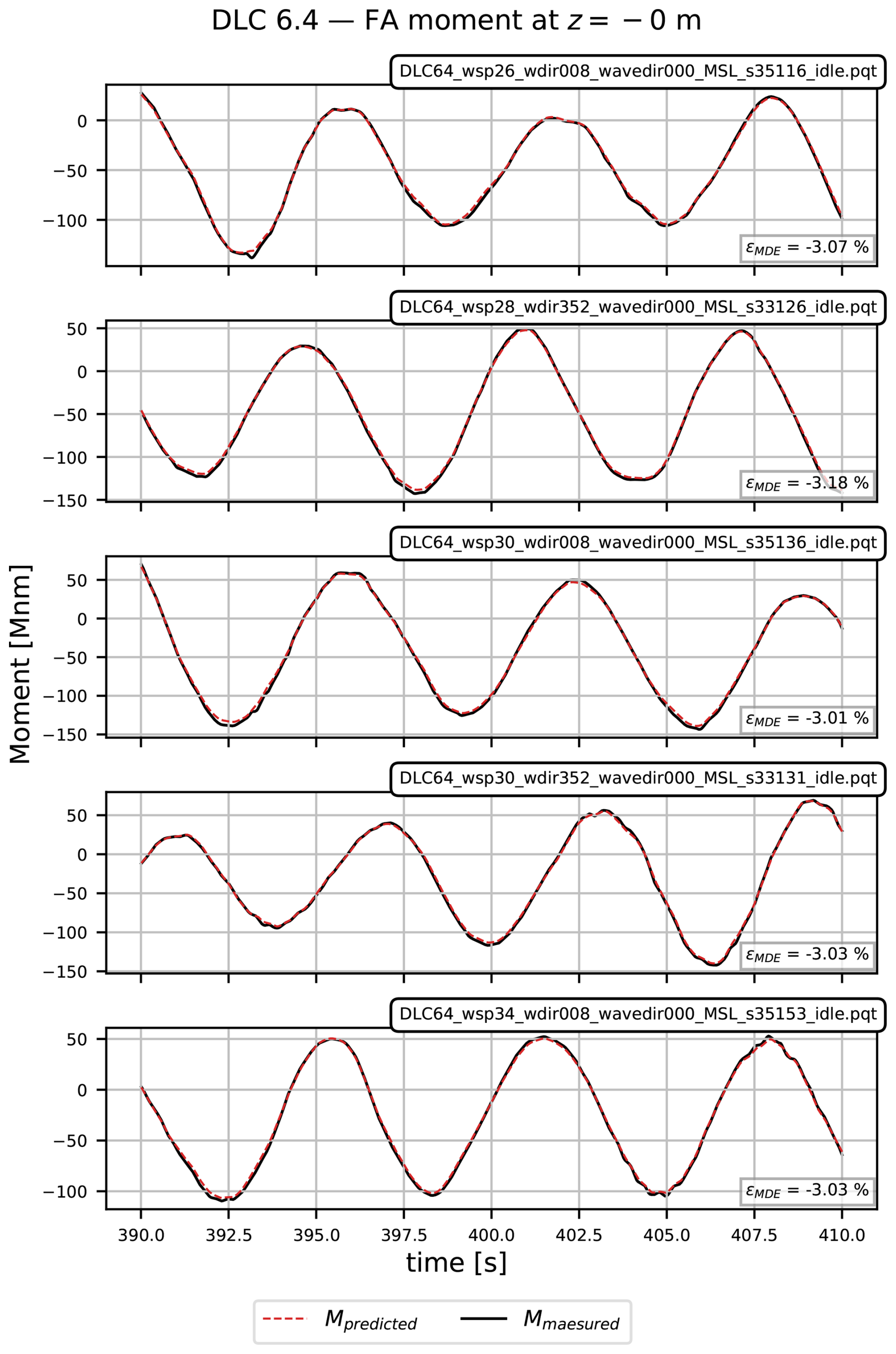
Figure C8 Segments of selected FA moment histories corresponding to the largest relative MDE errors (ε_MDE) at the 0 m above MSL elevation for DLC 6.4. The time series segments include (1) the predicted moment history (red) and (2) the true (or measured) moment history (black).