Wake steering under inflow wind direction uncertainty: an LES study

Wake steering through static yaw control is a promising wind farm flow control strategy; however, full-scale implementation in real wind farms is hampered by uncertainties not typically present in a simulation environment. The most notable of these are bias and variability in inflow wind direction – which are both inherent in the atmosphere and introduced through imperfect measurements. To investigate the impact of these uncertainties, large-eddy simulations (LES) are conducted on a row of four turbines in a conventionally neutral boundary layer, using three yaw configurations (an unyawed baseline, the leading turbine yawed and the first three turbines yawed) under different mean inflow wind directions $\in [-\mathrm{5},\mathrm{8}]\mathit{°}$. The impact of the applied yaw strategy and mean wind direction offset is first studied, considering the asymmetry introduced by veer, mean wake shape, changes in local inflow angle, and individual turbine power and loads. Considering mean wind farm power output, the inflow wind direction standard deviation in the current study (σ_WD = 2.3°) results in a beneficial window for wake steering of 8.5° ($\in [-\mathrm{1.5},\mathrm{7.0}]\mathit{°}$) with peak total power gains of 23 % and 7.5 % for the two yaw strategies, respectively. Therefore, an error in assumed or measured mean inflow wind direction of ∼ 4° could turn a promising prediction into an actual power loss. Extrapolating to an uncertainty of σ_WD = 4.5° using a Gaussian convolution reduces the beneficial ranges to 8 and 6.5°, respectively, with peak gains reduced to 7.5 % and 2 %. While exact numbers depend on turbine spacing, the substantial decrease in peak power and narrow range of power gains signify that wake steering is highly sensitive to wind direction uncertainty and small biases in mean inflow wind direction, even in favourable atmospheric conditions. Therefore, accurate measurement of these quantities and inclusion of them in prediction models is essential to the operational implementation of wake steering.

1 Introduction

Wake effects – namely lower mean velocity and higher turbulence intensity – cause power losses and fatigue increases in wind farms when wind turbines operate in the wakes of those upstream. Wind farm flow control (WFFC) involves altering the operation of individual turbines in order to reduce wake-induced losses in a wind farm, and hence improve overall metrics such as total power production (Meyers et al., 2022). Static yaw control is a WFFC technique that consists of applying a constant yaw misalignment angle to a turbine nacelle relative to the incoming flow. This produces the effect of wake steering, in which the asymmetry in the rotor loads imparts forces on the flow which lead to deflection of the mean wake centreline in the crosswind direction. Therefore, in aligned or nearly aligned flow scenarios with significant wake effects, wake steering could be applied to redirect the wakes of upstream turbines and hence increase the mean inflow velocity and power output of downstream turbines (Jiménez et al., 2010). However, static yaw results in a power output and fatigue penalty for the turbines it is applied to (Hulsman et al., 2020; Debusscher et al., 2022), hence identifying exactly where and how to utilise wake steering when WFFC is in reality non-trivial.

This is in particular due to the complex, three-dimensional and dynamic nature of wind turbine wake behaviour and wind farm flows. Wake recovery – and hence the effectiveness of applying wake steering – is significantly impacted by ambient turbulence intensity (Wu and Porté-Agel, 2012; Churchfield et al., 2012), veer (van der Laan and Sørensen, 2017) and turbulence integral length scale (Du et al., 2021; Hodgson et al., 2023a), which are driven by atmospheric stability. Wind farm flows also include interactions with the size and layout of the wind farm (Cortina et al., 2016; VerHulst and Meneveau, 2014; Andersen et al., 2017) and with the atmospheric boundary layer (Allaerts and Meyers, 2017; Abkar and Porté-Agel, 2015). The asymmetry introduced by yawing further complicates wake physics by introducing a counter-rotating vortex pair which deflects the wake and modifies the mean wake shape to a curled (or “kidney”) shape (Mikkelsen, 2004; Howland et al., 2016). This leads to further interactions with wake rotation and veer, which lead to anticlockwise yaw (as seen from above) being more effective in the Northern Hemisphere (Fleming et al., 2018; Archer and Vasel-Be-Hagh, 2019; Narasimhan et al., 2022).

Even once appropriate conditions for applying static yaw control have been identified in a theoretical, quasi-static sense – a wind farm with relatively close spacing, aligned mean inflow wind direction, below-rated velocity and low ambient turbulence intensity – significant challenges remain when implementing yaw control in a practical context. Sources of uncertainty exist in both the application of the intended control strategy and the measurement of inflow conditions which the strategy relies on. Concerning the application of the intended control strategy, the response to control inputs is affected by time lags and low speed of yaw actuation, and large deadband zones in individual turbine yaw controllers lead to imprecise tracking of the mean inflow angle. Yaw position uncertainty has been reported both as a Laplacian distribution with a scale factor of ν = 6.16° (Quick et al., 2020) and Gaussian distributed with a standard deviation of 1.75° (Simley et al., 2020). Regarding the measurement of inflow conditions, using e.g. nacelle anemometers and wind vanes can introduce bias and uncertainty due to sensor drift and error, which are exacerbated in yawed conditions due to calibration issues and flow distortion around the nacelle. Additionally, inflow conditions have an inherent uncertainty due to turbulence and inhomogeneity of background flow conditions over the extent of a wind farm. Reported values of wind direction uncertainty (the short-term variability within 1–10 min periods) typically range from 2.5 to 6°: 2.7° from 10 min sonic anemometer data from an offshore wind farm (Gaumond et al., 2014), 3.6° predicted from 10 min turbine sensor data (Mittelmeier et al., 2017), and 5.15 and 5.2° using 1 min averages for two different onshore locations (both a combination of yaw position and wind direction uncertainty), with much larger values for wind speeds of less than 8 m s⁻¹ (Simley et al., 2020, 2021). Spatial variability in mean values can also be significant; the difference in wind direction (without wind farms present) was found to have quartiles of −1.5 and 1.3° on an intra-cluster scale (∼ 10km, and −3.8 and 5.0° on an inter-cluster scale (∼ 50km) using New Europe Wind Atlas (NEWA) data in Von Brandis et al. (2023).

The range of inflow wind directions over which yaw control is predicted to be beneficial varies between setups, depending on turbine spacing and the flow model used in the prediction. In field experiments, yaw predictions are typically made using engineering models, such as implemented in FLORIS (Gebraad et al., 2016) or PyWake (Pedersen et al., 2023). Typical ranges over which yaw is applied are $\sim [\mathrm{0},\mathrm{25}]\mathit{°}$ if only one yaw direction is considered (Fleming et al., 2019, 2020) or $\sim [-\mathrm{20},\mathrm{20}]\mathit{°}$ for both directions (Doekemeijer et al., 2021), with large yaw angles (e.g. > 15°) occurring in a smaller range ($\sim [\mathrm{0},\mathrm{10}]\mathit{°}$ or $\sim [-\mathrm{10},\mathrm{10}]\mathit{°}$). When attempting to evaluate the impact of the applied strategy, results are binned by wind speed and direction, and the inactive and active control periods are compared within each bin. In order to ensure enough data per bin, and not to over-resolve relative to measurement uncertainties, wind direction bin widths are typically 3–5° (Göçmen et al., 2022; Fleming et al., 2020; Doekemeijer et al., 2021). This is relatively large in comparison to the predicted beneficial wind direction window for wake steering. Additionally, optimal yaw setpoint predictions often display a discontinuous change in yaw misalignment with wind direction (e.g. through a change in sign) around fully aligned conditions, as the models predict a “breaking point” where it is optimal to yaw the turbine in the opposite direction (Rott et al., 2018). This leads to a very high sensitivity in the desired yaw position in exactly the area where potential gains (and potential losses if incorrect control is applied) are highest.

Rott et al. (2018) attempt to address both the issues related to discontinuities in yaw setpoint and wind direction uncertainty by proposing applying a Gaussian convolution to the predicted setpoints from engineering models, which both reduces the high gradients around fully aligned conditions and the magnitude of predicted yaw angles. Simley et al. (2020) used a similar approach to achieve a better fit between numerical and experimental data by proposing that the achieved yaw offsets were a convolution of the Gaussian yaw error distribution and the intended yaw setpoints. Kanev (2020) suggests a hysteresis-based approach to reduce the turbine yaw duty due to sign changes in optimal angle. In Quick et al. (2020), the impact of five sources of uncertainty on yaw optimisations were studied: yaw position, wind direction, wind speed, turbulence intensity and shear, with the former two found to be the most impactful. The largest overall impact was that of wind direction uncertainty, with larger values leading to a greater spread in the possible wake area, therefore increasing baseline (unyawed) power production and decreasing the optimal yaw setpoint. However, assessing uncertainties only using engineering wake models has some drawbacks. Engineering models generally only include the impact of turbulence implicitly through wake expansion coefficients (Peña et al., 2016) and so do not capture the effect of wake dynamics such as far-wake meandering (Larsen et al., 2008; Medici and Alfredsson, 2006). Many models do not include the curled mean shape of a yawed wake and can also struggle to correctly capture wake deflection (Steiner et al., 2025). Additionally, the asymmetry between effectiveness of anticlockwise and clockwise yaw angles, and the interaction of the wake with veer, are not modelled. All of these factors may affect how wind direction uncertainty is predicted to impact the wind farm flow and total power output.

Therefore, this work aims to address the issue of wake steering under inflow wind direction uncertainty using large-eddy simulations (LES). By utilising a conventionally neutral boundary layer (CNBL) inflow, and an aero-servo-elastic coupled actuator disc for turbine modelling, the wakes, wind farm flow, power and loads can be studied while including the effect of dynamic wake behaviour and turbulent inflow, and interaction with shear and veer. However, while LES allow atmospheric boundary layers to be used as inflow, these do not include the impact of meso-scale variations and instead typically use a constant geostrophic wind to drive the flow, resulting in less variability in inflow velocity and direction than in field experiments. Hence, a number of inflow wind directions are simulated in order to study both the impact of bias (e.g. an error between the assumed and actual mean wind direction) and uncertainty (e.g. short-term variability) in inflow wind direction. Rotating the wind farm coordinates means that different wind directions can be simulated using an identical inflow, and hence the effect of the incoming wind direction can be isolated. A row of four turbines is simulated with three different yaw configurations: a baseline with no yaw; the leading turbine yawed anticlockwise by 20°; and the first three turbines yawed anticlockwise by 20°. Six different inflow wind directions are simulated: $[-\mathrm{5},-\mathrm{3},\mathrm{0},\mathrm{3},\mathrm{5},\mathrm{8}]\mathit{°}$. First, the flow is studied: wake deflection, wake shape, local inflow angle and their development through the turbine row. Then, the individual turbine power and loads are addressed, and finally the total wind farm power output and impact of wind direction bias and uncertainty are examined.

2 Methodology

2.1 Flow solver

All simulations are conducted using EllipSys3D, a general purpose multi-block Navier–Stokes solver developed at the Technical University of Denmark (DTU) (Sørensen, 1995; Michelsen, 1992, 1994). EllipSys3D solves the incompressible governing equations with a finite volume method in general curvilinear coordinates using a collocated grid. The potential temperature transport equation is also solved, as a conventionally neutral boundary layer (CNBL) is utilised as inflow and hence temperature effects are included in simulations. An extended SIMPLEC algorithm solves the pressure correction equation (Shen et al., 2003; Kobayashi and Pereira, 1991) with Rhie/Chow interpolation, and time advancement is performed with a second-order accurate three-level implicit method including sub-iterations in each time step. A fourth-order central differencing scheme discretises the convective terms, with a fourth-order dissipation term to reduce numerical instabilities (Wit and van Rhee, 2013). Turbulence modelling is achieved using LES with the AMD subgrid scale model (Abkar et al., 2016). Log law is applied at the lowest grid cell to calculate the instantaneous shear stress.

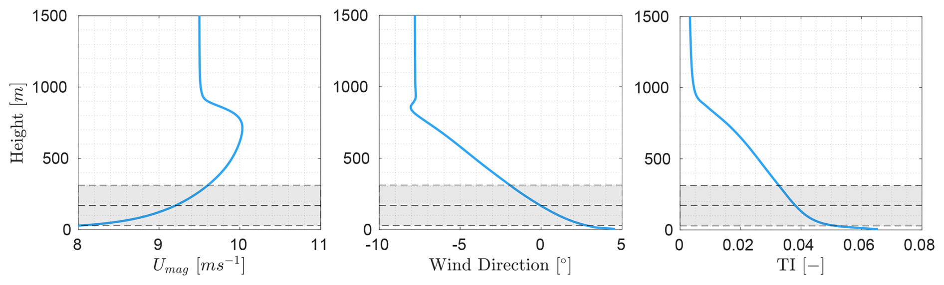
Figure 1 Horizontally and time-averaged profiles of the CNBL precursor inflow: (A) velocity magnitude U_mag (m s⁻¹), (B) wind direction (°), (C) turbulence intensity (TI) based on hub height mean velocity. Area marked in grey represents the turbine rotor extent.

2.2 Wind turbine modelling

The IEA22MW reference wind turbine is used in this work, which has a diameter of D = 284 m and a rated power of 22MW (Zahle et al., 2024). Wind turbines are modelled in LES using the actuator disc (AD) method (Mikkelsen, 2004), which is coupled to the aero-servo-elastic solver HAWC2 (Larsen and Hansen, 2007) through the open-source python coupling framework Dynamiks (Pedersen et al., 2026). Dynamiks extracts the velocity components along the positions of the three rotating blades from EllipSys3D and passes them to HAWC2, which calculates loads and deflections using a blade-element momentum (BEM) approach based on tabulated aerofoil data, and uses the modified AD tip correction described in Pirrung et al. (2020). HAWC2 has a multi-body formulation based on Timoshenko beam elements and is able to account for non-linear effects of large deflections. The calculated loads and deflections of each blade are transferred back to EllipSys3D and used to set the position and magnitude of the body forces which make up the AD. These AD body forces are applied to the computational grid in three overlapping 240° sections, in which the forcing decreases linearly from a maximum at the blade location to zero at the neighbouring blades. A one-dimensional Gaussian smearing is also applied in the streamwise direction. This aeroelastic-coupled AD formulation, built from three overlapping sectors each representing a single blade, therefore resembles an azimuthally smeared actuator line or actuator sector. Hence, it is different from conventional AD approaches, which often use uniform loading or a rotor-element approach based on aerofoil data (Wu and Porté-Agel, 2011). The AD used here has been validated against the aeroelastic-coupled actuator line model (Hodgson et al., 2021) and other LES codes (Hodgson et al., 2023b), and results in very close alignment with the actuator line in terms of blade loading and thrust coefficient C_T. Therefore, the near-wake breakdown and wake development is also well represented, despite the fact that the AD results in a shear layer rather than tip vortices, being shed from the rotor disc (Hodgson, 2023). It allows non-uniform loading (e.g. due to shear and/or yaw) and its impact on both turbine response and wake to be captured. The two-way nature of the coupling means that the interaction between loading, deflections and flow is also represented (Hodgson et al., 2021). Additionally, HAWC2 uses the DTU Wind Energy Controller (Hansen and Henriksen, 2013), meaning that the turbine exhibits realistic changes in rotational speed and pitch in response to the turbine operation and loading. No individual turbine yaw controller is included, as the setup assumes zero nacelle orientation error in relation to the mean freestream wind (see Sect. 2.4), and the secondary steering effects are not large enough to trigger a realignment of downstream turbines (see Sect. 3.1, Fig. 5).

2.3 Atmospheric boundary layer precursor

One inflow is used for all simulations, consisting of 5100 s of a conventionally neutral boundary layer (CNBL). The CNBL is generated using a precursor simulation in LES, using a domain size of 16 640 m × 16 640 m × 3000 m (in streamwise, spanwise, vertical, respectively) with periodic boundary conditions applied on lateral and streamwise faces and a grid resolution of $\mathrm{d}x=\mathrm{d}y=\mathrm{2}\mathrm{d}z$ = 20 m, with moderate grid stretching applied in the z direction above 1500 m. This leads to a total mesh size of approximately 266 million cells. Rayleigh damping is applied above a height of 2000 m (Klemp and Lilly, 1978). At the ground, the log law is applied to the velocity field at the lowest vertical cell centres to calculate the instantaneous shear stress. The precursor is initialised with the following conditions: a temperature profile which is a constant T₀ = 288.15 K until 600 m height, with perturbations up to 100 m height to encourage breakdown into turbulence, then a linear gradient of $\mathrm{d}{T}_{\mathrm{0}}/\mathrm{d}z$ = 1 K km⁻¹ above, geostrophic wind values U_G = 9.48 m s⁻¹ and V_G = −0.59 m s⁻¹, and velocity profiles based on a log law with a 600 m boundary layer height (Allaerts and Meyers, 2015). Conditions constant throughout the precursor are the Coriolis parameter f_c = 1.1947 × 10⁻⁴ s⁻¹, wall roughness z₀ = 0.001 m, wall temperature T_wall = 288.15 K and geostrophic wind magnitude $\sqrt{(U_{\mathrm{G}}^{\mathrm{2}}+V_{\mathrm{G}}^{\mathrm{2}})}$ = 9.5 ms⁻¹. These conditions (and the resulting boundary layer flow) are designed to represent offshore conditions in northern Europe (Peña, 2019; Türk and Emeis, 2010). A wind direction controller is also active, which alters the geostrophic wind components in order to obtain a fully aligned flow (0°) at the turbine hub height of 170 m. The time step used is 1 s. The precursor is spun up over of flow time of 28 h, over which the boundary layer and turbulence develops. Then, another 5100 s of flow time is run, over which the three velocity components and temperature are extracted over a streamwise plane spanning the entire domain in vertical and lateral extent. These data are then used as the inflow to the successor simulation containing the turbines. Figure 1 shows the horizontally and time-averaged profiles of the CNBL over the 5100 s used as inflow to the successor simulation. The achieved inflow has below-rated velocity, a fully aligned mean wind direction at hub height (−0.05°), mild veer (4.5° over the rotor area) and a relatively low hub height TI of 3.8 %. Therefore, the simulated atmospheric conditions are ideal for the application of wake steering and hence allow the uncertainties that are present even in such favourable conditions to be investigated.

2.4 Simulation setup

All successor simulations utilise the same computational domain, which has dimensions of 13 490 m × 4970 m × 3000 m (47.5D × 17.5D × 10.5D). Following the precursor setup, Rayleigh damping is applied above 2000 m height, log law is used to calculate the instantaneous shear stress at the lowest vertical cell centres and the two lateral domain boundaries are modelled as periodic. The refined region extends from the inlet to 9940 m (35D) downstream, with lateral extent of 2840 m (10D) centred on the domain centreline and extending vertically from the ground to a height of 1136 m (4D). Inside the refined region, the grid resolution is $\mathrm{d}x=\mathrm{d}y=\mathrm{d}z$ = $D/\mathrm{32}$, a resolution sufficient to converge both the turbine thrust coefficient and wake behaviour (Hodgson et al., 2021, 2023b). Outside of the refined region, the cell sizes are stretched to the domain boundaries, and the total mesh size is approximately 116 million cells. The simulated wind farm consists of a row of four turbines spaced 7D apart, with the leading turbine placed 3.5D from the inlet and hence the final turbine being placed 11.5D (1.5 times the turbine spacing) before the end of the refined region. All simulations are run for 5100 s of flow time, in which the first 1500 s (the time taken for a full flow-through of the computational domain at U_hub, or a full flow-through of the refined region at 0.7U_hub) are used as spinup to develop the flow and wakes. The last 3600 s are used for analysis, and the flow solver time step is 0.5 s.

In order to examine wake steering wind farm flow control, three different yaw configurations are examined: the first, a baseline case where no yaw is applied; second, a single-turbine yaw case where the upstream turbine is yawed −20°; and third, a multi-turbine yaw case where the first three turbines are yawed −20°. Note that a negative yaw direction in this context refers to the turbine rotating anticlockwise when seen from above and hence is the direction which produces more beneficial wake steering in the Northern Hemisphere due to the interaction between turbine yaw, wake rotation and veer (Fleming et al., 2018; Archer and Vasel-Be-Hagh, 2019). This work investigates both mean wind direction bias (a constant offset, which is what is simulated) and standard deviation (both included and extrapolated to larger values from the obtained results). As the mean wind direction is unaltered in the LES, the wind farm coordinates are rotated to achieve a change in wind direction relative to the wind turbine row. Note that the wind turbines still face directly into the incoming wind, and hence this simulates a situation with zero error in the individual turbine nacelle orientations. Six different inflow wind directions (and therefore coordinate rotations of the wind farm) are studied: $[-\mathrm{5},-\mathrm{3},\mathrm{0},\mathrm{3},\mathrm{5},\mathrm{8}]\mathit{°}$. Consistent with the yaw rotation definition, a positive wind direction indicates a clockwise rotation of the incoming wind relative to a fully aligned inflow.

In order to achieve a fair comparison, the available power outputs and inflow angles at each of the turbine locations (e.g. in each coordinate configuration) should be identical, so that results can be attributed to the simulated inflow wind direction rather than the turbine locations. Therefore, initial simulations were run – one set without turbines present and another with only the first turbine present – to assess the dependency of inflow angle, wind speed and first turbine power output on location. Mean velocity matched to 0.1 % between each turbine location in the empty domain, and power output for the first turbine changed less than 0.5 % – consequently, this defines the minimum level of power change that can be judged as significant in the results. For the inflow angle, across all turbine locations in the empty domain, the hub height values are between −0.15 and 0.15° (the mean horizontally averaged value during the last 5100 s of the precursor was −0.05°). This minimal variation around 0.0° was judged as sufficient to say that the six desired wind directions ($[-\mathrm{5},-\mathrm{3},\mathrm{0},\mathrm{3},\mathrm{5},\mathrm{8}]\mathit{°}$) are achieved by the coordinate rotations.

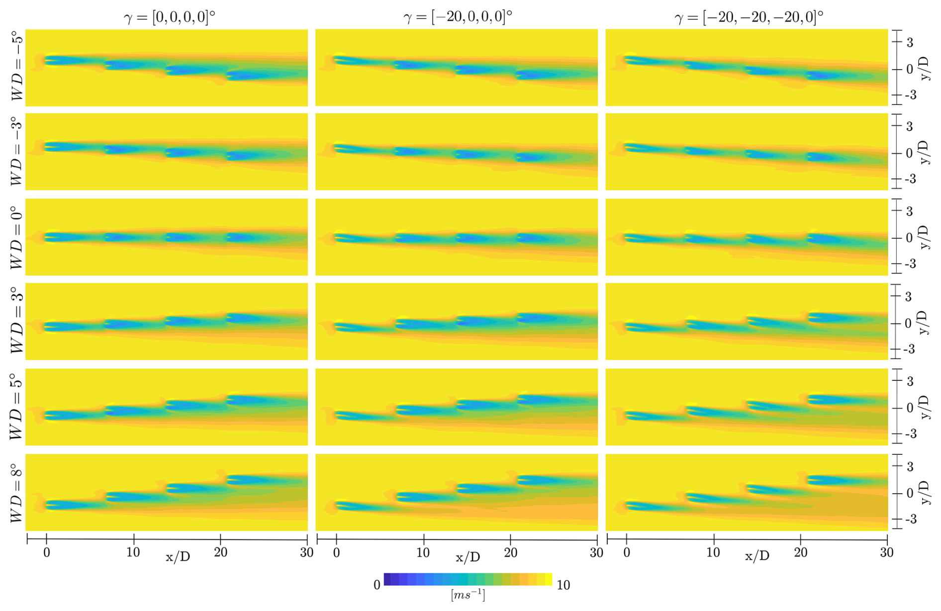
Figure 2 Contour plots using horizontal plane at turbine hub height of U_mag (m s⁻¹) for all wind directions, showing baseline case with no yaw (left), yawed case with first turbine yawed −20° (middle) and yawed case in which the first three turbines are yawed −20° (right). From top to bottom: −5, −3, 0, 3, 5, 8°.

3 Results

3.1 Wind farm flow

The impact of the different inflow wind directions on the wind farm flow is first qualitatively examined by comparing the mean flows across a horizontal plane at hub height for all wind directions and all yaw configurations, shown in Fig. 2.

Figure 2 demonstrates how the coordinate rotations of the wind farm allow different inflow wind directions to be simulated. The third row, first column simulation ($\text{WD}=\mathrm{0},\mathit{\gamma }=[\mathrm{0},\mathrm{0},\mathrm{0},\mathrm{0}]\mathit{°}$) shows the baseline case in which the wind direction is fully aligned with the turbine row and no yaw is applied. There is already flow turning through the farm in this case, due to the interaction of the wakes with the inflow veer (van der Laan and Sørensen, 2017). As shown in Fig. 1, the veer is ∼ 4.5° over the rotor area and the boundary layer height is around 900 m. This veer is relatively low compared to stable times of day with lower boundary layer heights (e.g. as simulated in a diurnal cycle inflow in Hodgson et al., 2025a, or a CNBL in Ivanell et al., 2025) and hence even stronger effects could be present with other inflow conditions. Wind directions of WD = $[-\mathrm{5},-\mathrm{3},\mathrm{3},\mathrm{5}]\mathit{°}$ represent partial wake cases, where in the unyawed configuration, the mean wake from each turbine impinges on the rotor area of the following. By comparing the unyawed configurations of WD = −5 and 5°, and −3 and 3°, the asymmetry of the wind farm flow introduced by the veer can be seen, as the negative inflow wind directions lead to greater wake impingement, due to the flow turning through the row. The largest wind direction offset WD = 8° shows very little wake impingement on downstream turbines in the unyawed configuration (this of course depends on the turbine spacing in addition to the angle). It is therefore likely that with this large a bias in wind direction, the yawed configurations at WD = 8° will give a total power loss due to the power reduction for yawed turbines. It is also apparent that the yawed configurations in cases WD = −5° and WD = −3° will result in a loss, as the applied yaw acts to steer the wakes into the downstream turbines, turning a partial wake case into a full wake.

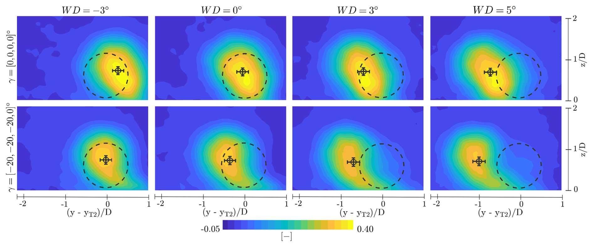
Figure 3 Contour plots using cross-stream plane at 0.5D in front of Turbine 2, showing mean normalised velocity deficit, $\left(U\right(z{)}_{\text{in}}-U)/U(z{)}_{\text{in}}$ velocity. Mean wake centre position and error bars showing standard deviation of wake centre in black. Dashed circle represents the rotor position and area of Turbine 2. Top row: baseline cases without yaw; bottom row: first three turbines yawed. From left to right: wind directions of −3, 0, 3, 5°. Planes oriented as seen from behind.

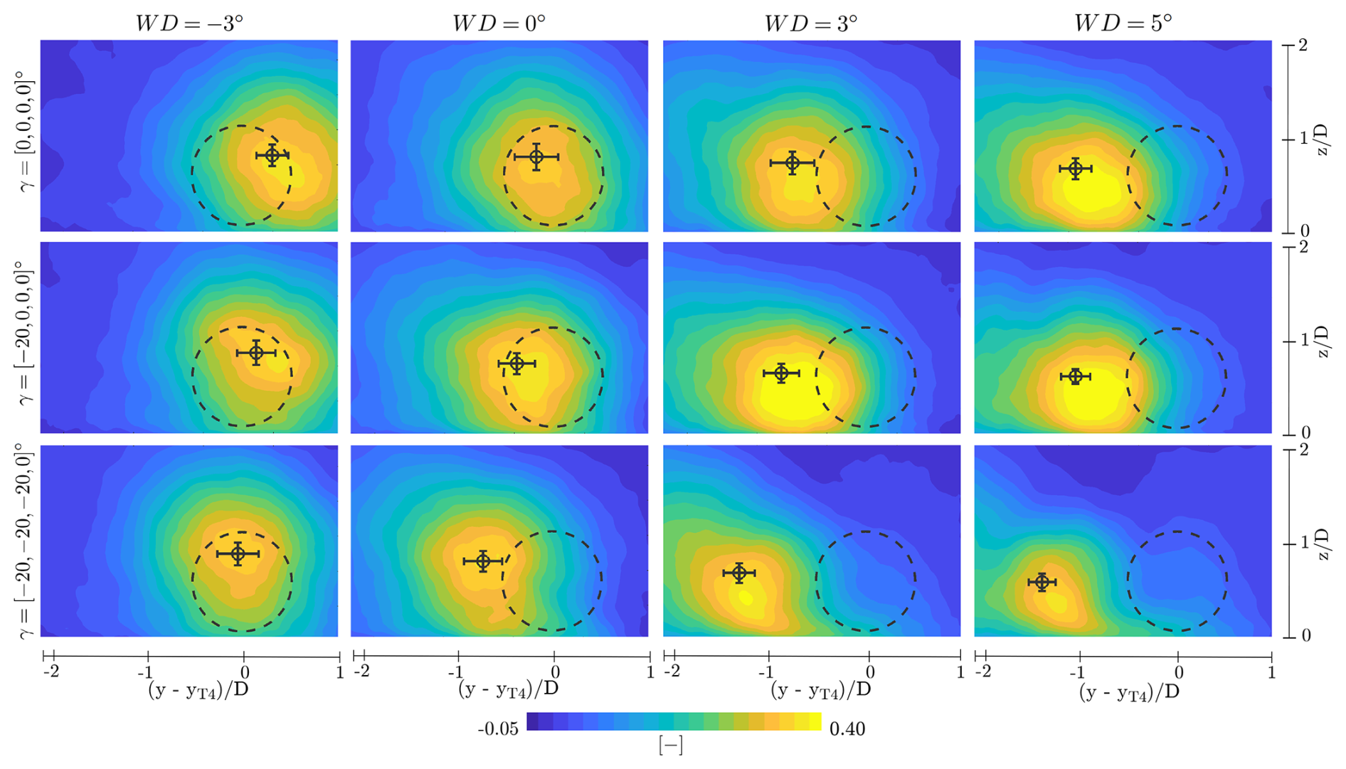
Figure 4 Contour plots using cross-stream plane at 0.5D in front of Turbine 4, showing mean normalised velocity deficit, $\left(U\right(z{)}_{\text{in}}-U)/U(z{)}_{\text{in}}$ velocity. Mean wake centre position and error bars showing standard deviation of wake centre in black. Dashed circle represents the rotor position and area of Turbine 4. Top row: baseline cases without yaw; middle row: first turbine yawed; bottom row: first three turbines yawed. From left to right: wind directions of −3, 0, 3, 5°. Planes oriented as seen from behind.

To examine the mean wake shapes and wake deflection, Figs. 3 and 4 show the mean normalised wake deficit at 0.5D upstream from the second turbine location (Fig. 3) and the fourth turbine location (Fig. 4), with mean wake centres and standard deviations marked, calculated using a centre-of-mass approach (Andersen, 2014). Only the four most relevant wind directions are shown: WD = $[-\mathrm{3},\mathrm{0},\mathrm{3},\mathrm{5}]\mathit{°}$. It should be noted that Fig. 3 only shows one of the two yawed configurations as the second turbine inflow is effectively identical in these cases.

The impact of both veer and yaw on the mean wake shapes can be clearly seen in the inflow to Turbine 2 (Fig. 3). For the unyawed configurations (top row), a skewed mean wake deficit is visible, while the yawed configurations (bottom row) display a mean wake deficit which is both skewed and curled, as well as having a deflected mean centre position. As expected, the wake centre standard deviation due to wake meandering is larger in the lateral direction than the vertical (España et al., 2012). There is little noticeable difference between the standard deviations in the unyawed and yawed configurations, suggesting similar wake meandering for both. The yaw applied to the leading turbine deflects the wake centre by around 0.25D by the second turbine location in all cases.

In Fig. 4, the mean inflows contain a much broader area of velocity deficit than in Fig. 3, as these inflows are formed from the combined wakes of three turbines rather than one. The wake centre standard deviations are also larger than in Fig. 3, as the interaction of multiple wakes leads to larger and more chaotic motions. Additionally, there is little evidence of the skewed and curled mean shapes that are present for the first wake. As a turbine wake has additional turbulence and a velocity deficit, it changes the shear and veer profiles at the inflow to downstream turbines, meaning that their wakes do not display the same strong veer interaction as the leading wake. This also demonstrates that beyond the entry region of a wind farm, it is the characteristics of the wakes and wind farm rather than the ambient conditions that can begin to dominate the flow, as seen for turbulent spectra in Hodgson et al. (2025b) and Andersen et al. (2017). This is particularly the case for the more aligned wake cases, while for WD = 3° and WD = 5° cases, the curled shape can be seen when all three turbines are yawed (the rightmost two of the bottom row in Fig. 4). It is only because the wakes of the other turbines are already sufficiently deflected that the third turbine wake behaves closer to what is seen for freestream conditions.

After qualitatively analysing the mean wakes and the mean local inflows, the local wind direction at each turbine is assessed. Figure 5 shows area-normalised histograms (to make the total area unit magnitude) of the local wind direction, calculated from a point velocity which is sampled at hub height 0.5D in front of each turbine, after applying a 60 s moving mean on the 1 Hz signal. Note that 0.5D in front (or upstream) means a point in negative x direction relative to each turbine, rather than relative to the rotated centreline of the wind farm.

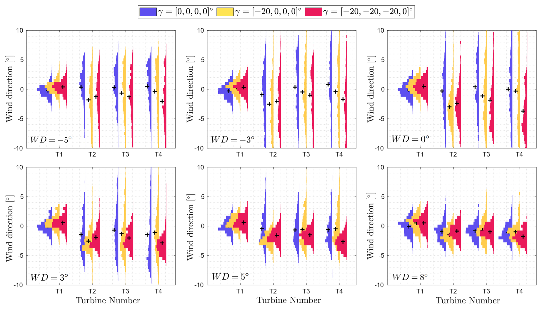
Figure 5 Area-normalised histograms of wind direction measured 0.5D upstream of each turbine location for all yaw scenarios and for each inflow wind direction. Black crosses indicate the mean of each distribution.

For all wind directions, the leading turbine in the baseline unyawed case has a wind direction with a mean at 0° and a relatively Gaussian distribution, as expected. There is a slight positive offset in the mean for all of the leading turbines in yawed configurations, presumably due to asymmetry introduced in the induction zone due to the yaw. The standard deviation of the freestream inflow distributions, using the 60 s moving mean, is σ_WD = 1.2°. However, the moving mean is applied to clarify the underlying trends in the distributions, and it is the standard deviation of the raw 1 Hz signal that gives the most appropriate value to compare with other work. The 1 and 10 min standard deviations of the raw 1 Hz freestream wind direction are similar: 2.4 and 2.3°, respectively. The 10 min freestream wind direction standard deviation σ_WD = 2.3° is therefore used to characterise the wind direction variability throughout this work.

It is clear that the distribution of inflow wind direction experienced by the first turbine is substantially different to that of downstream turbines that operate in wake. Particularly visible for the most aligned wake cases, WD = −3° and WD = 0°, the standard deviation of the wind direction is substantially increased by the presence of wakes, with a spread greater than ± 10°, while the spread at the first turbine inflow is ± 3°. Therefore, the presence of wakes generates large uncertainty in inflow wind direction for waked turbines, regardless of the uncertainty present in the ambient flow, as also shown in Andersen et al. (2015). The distributions of inflow wind direction also clearly demonstrate that, for this spacing of 7D, at WD = 8° there is very little wake impingement on the downstream turbines, as all distributions are similar in shape to that at the inflow to the first turbine.

The yaw misalignment also leads to a mean local wind direction offset at the turbine immediately downstream, due to not only deflecting the mean wake centre but also leading to a local redirection of the flow. For example, for WD = 0°, a difference in mean local wind direction of 3° is present at the second turbine; similar trends are reflected for all other wind directions. Additionally, when only the leading turbine is yawed (the yellow distributions), the local wind direction distribution converges towards the unyawed baseline by the end of the turbine row, while the largest difference in mean local wind direction occurs at the fourth turbine, in the configurations where three turbines are yawed.

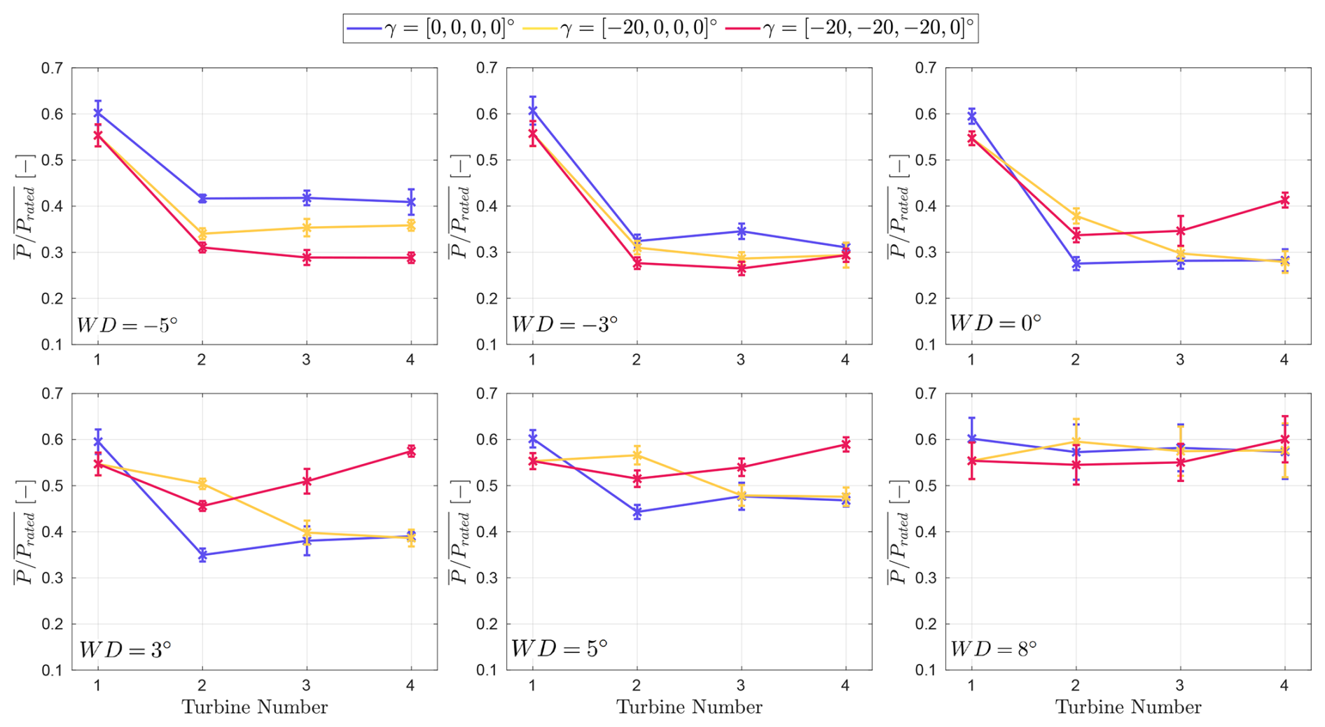
Figure 6 Mean and standard deviation of individual turbine power output across each turbine row for all yaw scenarios. Each plot shows a different inflow wind direction (as labelled).

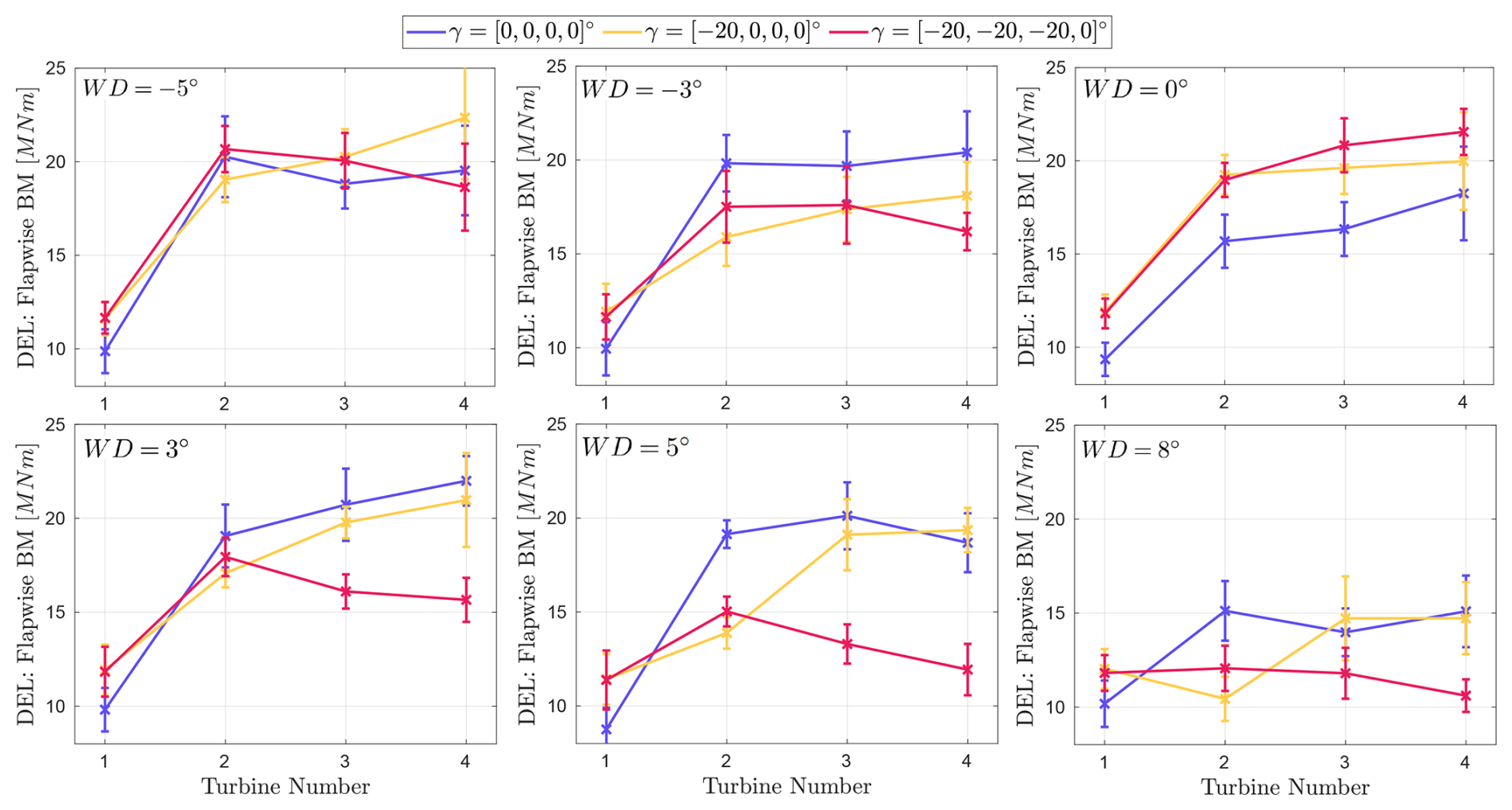
Figure 7 Mean and standard deviation of 10 min damage equivalent loads for flapwise blade root bending moment for individual turbines across each turbine row for all yaw scenarios. Each plot shows a different inflow wind direction (as labelled).

3.2 Individual turbine response

After examining the flow and local wind directions, the response of the individual turbines – in terms of power output and loading – can be examined. Figures 6 and 7 show the mean and standard deviation of power output and damage equivalent loads (DELs) of the flapwise blade root bending moment of each turbine in the row for all yaw configurations and all inflow wind directions. Damage equivalent loading is calculated from data at a frequency of 1 Hz over 10 min periods, staggered by 5 min, in order to generate 11 samples for the 1 h time period. The mean and standard deviation in Fig. 7 are of those 11 samples. The power output mean and standard deviations are likewise calculated from 10 min means of the raw 1 Hz data.

As expected, the leading turbine has the highest power output and the lowest damage equivalent loads, as it experiences the freestream inflow with higher velocity and lower turbulence intensity than the flow within the turbine row. Generally, after the first turbine, the individual turbine power output decreases and the flapwise DELs increase, depending on the degree of waked inflow. For the first turbine, yawing increases the flapwise DELs and reduces the power output. Similar to the mean local wind direction offset induced by wake redirection, the power output of the one-turbine yaw configuration converges towards the baseline through the row, which agrees with the conclusions of Archer and Vasel-Be-Hagh (2019) that yawing only the leading turbine is insufficient to achieve changes past two to three turbines downstream. In the three-turbine yaw configuration, for wind directions WD = 0° and WD = 3°, the most significant power gains compared to the baseline occur at the last turbine, showing the importance of the cumulative gains.

The trends in power output confirm the qualitative conclusions from the mean flow plots in Fig. 2 – that for negative wind directions, yawing causes a power loss as it enhances rather than mitigates wake effects, and for a wind direction offset of 8°, there is very little wake interaction. For WD = 8°, the downstream turbines in the baseline case have a higher power output than the yawed leading turbine in the yawed configurations. This case clearly exists past the boundary for beneficial application of wake steering for this wind farm, as the losses due to the power–yaw relation exceed the wake losses present in the baseline. The exponent α in the power–yaw relation has a value of 3 according to momentum theory but in reality varies between 1 and 3 for different turbines and waked states (Liew et al., 2020). Fitting the power–yaw relation to the first turbine loss at WD = 0° (so based on γ = 0° and γ = −20°) gives an exponent of α = 1.35, a low exponent which leads to a relatively small penalty for yawing compared to other turbines and the assumptions made in engineering wake models.

The DEL plots in Fig. 7 show that the maximum flapwise DELs occur in partial wake cases: for the unyawed configurations at WD = −3°, WD = 3° and the yawed configurations for WD = 0°. While yawing increases the flapwise DELs for an individual turbine, there are several wind directions in which the yaw strategy leads to reductions in total DELs over the turbine row: WD = −3°, WD = 3°, WD = 5° and WD = 8°. The DEL reduction for WD = −3° is due to moving from a partial wake to a full wake state, which is therefore accompanied by an undesirable power loss. However, for WD = 3°, WD = 5° and WD = 8°, the load reduction occurs through mitigation of the partial wake state by steering the wakes farther away from downstream turbines. These results are aligned with Bartl et al. (2018), in which yaw moment reductions were observed when partial wake states were mitigated. This is particularly interesting for WD = 8°, where flapwise DEL decreases are present for the three-turbine yaw scenario despite it resulting in total power losses. This decrease in flapwise DELs by mitigation of partial wake can be seen in the local inflow wind direction plots of Fig. 5, as the high spread of local wind direction for downstream turbines present in the unyawed configurations is significantly reduced in the yawed configurations.

3.3 Wind farm power output

Examining the wind farm power output allows the effect of applying wake steering and its sensitivity to inflow wind direction uncertainty to be established. Figure 8 shows the mean wind farm power output for all configurations, grouped by inflow wind direction. Error bars show the standard deviation of the instantaneous (1 Hz) wind farm power.

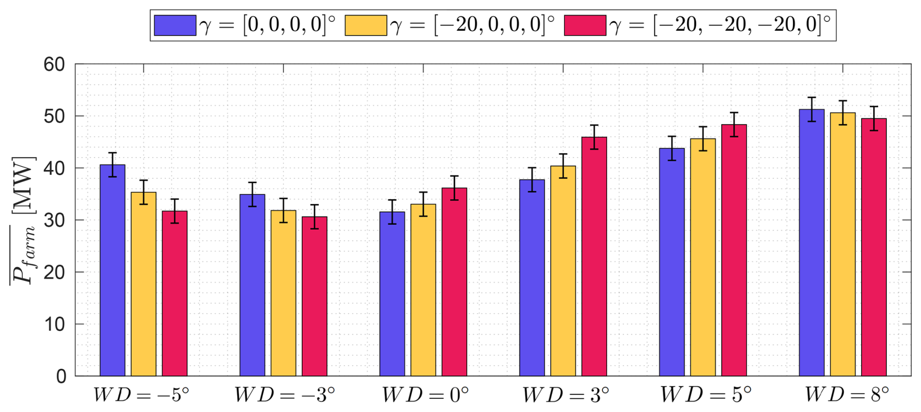
Figure 8 Mean wind farm power output for all cases. Error bars represent standard deviation of instantaneous (1 Hz) power.

As expected, the lowest wind farm power output of any unyawed configuration occurs at the fully aligned inflow conditions of WD = 0°, with increases in power output at both positive and negative wind directions due to the offset in inflow wind direction reducing the wake losses in the turbine row. The difference in power output between the unyawed configurations at WD = −3° and WD = 3° (2.8 MW, around 8 %), and WD = −5° and WD = 5° (3.2 MW, also around 8 %) shows the asymmetry introduced due to the wake interaction with veer, as otherwise the two pairs of cases are mirror images of one another.

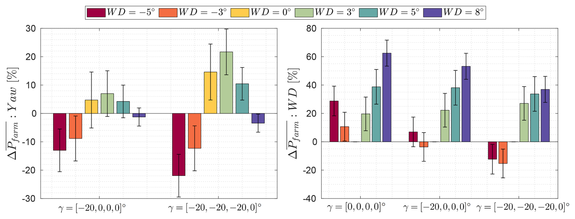
Figure 9 Differences in mean wind farm power output: (A) power difference due to yawing (e.g. difference relative to unyawed baseline case); (B) power difference due to wind direction offset (e.g. difference relative to WD = 0° case). Error bars represent the standard deviation of the instantaneous (1 Hz) power difference.

To clarify the power changes between yaw configurations and wind directions, Fig. 9 shows the difference in mean wind farm power output. Figure 9A shows the power change between the yawed and unyawed configurations (e.g. the power change due to applying wake steering) for all wind directions; Fig. 9B shows the power change between the non-zero inflow wind directions and the fully aligned case (e.g. the power change due to the offset in inflow wind direction) for all yaw configurations. Including both plots is important because it is interesting to note the relative size of the power output change caused by the two effects. Error bars on both plots show the standard deviation of the instantaneous (1 Hz) difference between cases, therefore representing the 16th and 84th percentiles of the distributions (which are Gaussian in shape).

Figure 9A shows that yawing either the first turbine, or the first three turbines, leads to wind farm power gains for wind directions WD = 0, 3 and 5°, and losses for WD = −5, −3 and 8°. Peak power gains occur at a mean wind direction of 3°. Yawing three turbines rather than one leads to greater potential power output gains at beneficial inflow wind directions but also greater losses at disadvantageous ones. However, the ratio between losses and gains (e.g. between power gain at WD = 3° and power loss at WD = −3°) is better when yawing three turbines. Hence, this yaw configuration is more promising despite the higher sensitivity to inflow wind direction. Additionally, the high standard deviation of the instantaneous power change indicates that if power losses should be avoided, then even the maximum gain in the one-turbine yaw configuration is insufficient to ensure this. However, for the three-turbine yaw case, within one standard deviation of the mean, a power gain is still predicted for WD = 0°, WD = 3° and WD = 5°. The standard deviation is largest for WD = 0° in both yaw configurations and decreases with increasing wind direction as the wake effects within the turbine row decrease.

The maximum percentage gain in wind farm power output due to yaw is 22 %, achieved by yawing the first three turbines when the inflow wind direction angle is 3°. This percentage increase is similar to the impact of around a 2–3° change in inflow wind direction, as shown in Fig. 9B. For the unyawed configuration, there is a change in wind farm power output of 20 % between inflow wind directions of 0° and 3°, and an additional 18 % between 3 and 5°. This underlines two somewhat competing conclusions: first, the significant power losses due to wake effects in an exactly fully aligned case and hence the importance of mitigating such losses; and second, the high degree of certainty that is required about the mean wind direction if wake steering is to be applied. It is a relatively small range of wind directions that result in significant wake losses for this wind farm (and therefore large power gains from wake steering), and the wind farm power output in an unyawed state increases regardless of yaw when a small wind direction offset is present.

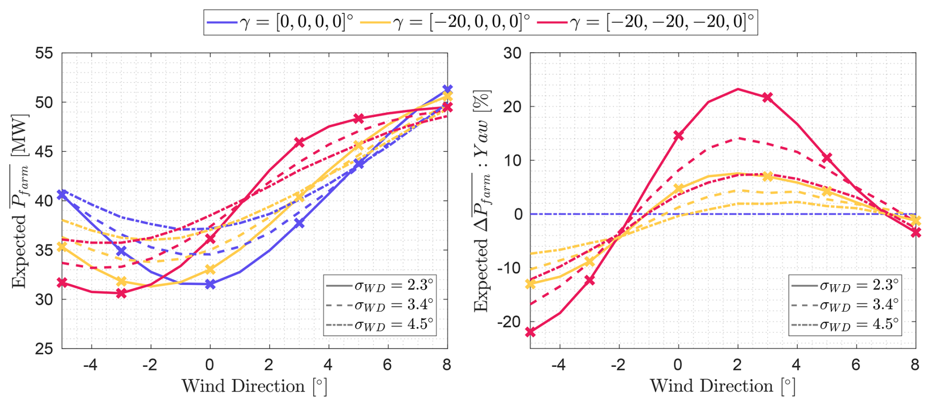
Figure 10 Impact of inflow wind direction uncertainty on wind farm power output: (A) mean wind farm power output under different wind direction uncertainties and yaw configurations, with crosses indicating LES data points (from Fig. 8), solid lines showing a fitted spline through the LES results and dashed lines giving predicted results from different wind direction standard deviations; (B) percentage difference in mean wind farm power output for each wind direction uncertainty, with crosses showing LES data points (from Fig. 9A), solid lines showing a spline fit to the LES results and dashed lines giving predicted results under different wind direction standard deviations.

Finally, using the mean wind farm power output results from different wind directions, the sensitivity of power output to inflow wind direction uncertainty can be established. This is achieved by firstly fitting a spline to each of the mean wind farm power output to inflow wind direction relationships for each yaw configuration (the data points in Fig. 8). In order to improve the spline gradients at the extreme points, WD = −5° and WD = 8°, additional data points are added at WD = −12° and WD = 10°, at which the turbines are assumed to operate completely in freestream. As a result, the farm has a total power which can be calculated from summing the mean powers of the unyawed and/or yawed states of the leading turbine. The splines exactly pass through each LES data point. These splines (one for each yaw configuration) represent the wind farm power output response under an inflow wind direction uncertainty of σ_WD,LES = 2.3°, which is the 10 min standard deviation of the freestream wind direction at the inflow to the first turbine. This value is inherent in the LES, arising due to the turbulent variations in the simulated atmospheric boundary layer. However, the purpose of simulating many wind directions is to expand the conclusions to the larger values of wind direction uncertainty present at real wind farms, with values reported in literature between 2.5 and 6° (Gaumond et al., 2014; Mittelmeier et al., 2017; Simley et al., 2020, 2021). Therefore, the impact of larger inflow wind direction standard deviations σ_WD is simulated by applying Gaussian convolutions with different standard deviations to the original splines (Rott et al., 2018; Simley et al., 2020). As the un-convoluted results (e.g. the original splines) already include the inherent σ_WD = 2.3° from LES, the total σ_WD shown is calculated as ${\mathit{\sigma }}_{\text{WD}}=\sqrt{{\mathit{\sigma }}_{{\text{WD}}_{\text{LES}}}^{\mathrm{2}}+{\mathit{\sigma }}_{{\text{WD}}_{\text{ADDED}}}^{\mathrm{2}}}$, where ${\mathit{\sigma }}_{{\text{WD}}_{\text{LES}}}$ = 2.3°. These results are shown in Fig. 10A and show the expected value of mean wind farm power output for different yaw configurations and different wind direction uncertainties. The x axis represents the mean of the inflow wind direction (the bias), each line style represents a different standard deviation (the uncertainty) and each colour a different yaw configuration. Figure 10B shows the percentage difference in wind farm power output between the yawed and unyawed configurations for each wind direction uncertainty.

The solid lines and crosses in Fig. 10A are simply splines fitted to the LES results from Fig. 8 and hence show the same results. However, trends in each yaw configuration are demonstrated more clearly: that the unyawed configuration has a minimum power output at fully aligned conditions, while for the yawed configurations the minimum is essentially shifted by −1.5 or −3°, respectively – the amount of row misalignment equivalent to the achieved wake redirection. The inclusion of larger values of wind direction uncertainty leads to the flattening of the trends; for the unyawed baseline, wind direction uncertainty increases the expected power output at WD = 0°, as the contribution from the most aligned wind direction is decreased. Expected wind farm power output is also increased in the minima of the curves for the yawed configurations, but the gradient of power increase and the peak values are reduced.

Figure 10B shows the percentage difference between the yawed and unyawed configurations under different wind direction uncertainties. Therefore, this also represents the application of a Gaussian convolution to the wind farm power difference plots in Fig. 9. Again, the crosses show the LES results and hence the solid lines represent a spline fit to those values. Considering only the inherent σ_WD = 2.3° present in the LES, the predicted peak gain is 23 % at a mean wind direction of 2° for the three-turbine yaw case and 7.5 % also at a mean wind direction of 2° for the one-turbine yaw case. The range of inflow wind directions at which these wake steering regimes are beneficial are $\in [-\mathrm{1.5}\mathit{°},\mathrm{7}\mathit{°}]$ and $\in [-\mathrm{1}\mathit{°},\mathrm{7}\mathit{°}]$, respectively. However, with larger values of wind direction uncertainty, the expected power gains and range over which they are achieved decrease. An examination of Fig. 10A explains why this is the case: the expected power of the baseline unyawed configuration significantly increases with larger wind direction uncertainties, and therefore there is less to gain from wake steering. Additionally, the smoothing of the gradient in the yawed configurations due to the Gaussian convolution reduces the peak expected power, therefore further diminishing the difference between yawed and unyawed setups. The maximum expected power change decreases from 23 % and 7.5 %, respectively for the two yawed configurations at σ_WD = 2.3°, to 7.5 % and 2.0 %, respectively, at σ_WD = 4.5°. The range of positive power change is reduced to $\in [-\mathrm{1}\mathit{°},\mathrm{7}\mathit{°}]$ for the three-turbine yaw configuration and to $\in [\mathrm{0.5}\mathit{°},\mathrm{7}\mathit{°}]$ for the one-turbine yaw configuration. In addition to changing the size of the peak power change, the ratio between losses and gains is also detrimentally affected. While the peak is reduced from 23 % to 7.5 % in the three-turbine yaw case, the power losses outside of the beneficial range do not decrease as much, changing from −22 % to −12 % at WD = −5° and from −3.5 % to −3 % at WD = 8°. Therefore, the potential gains are decreased due to the uncertainty of the full wake state actually occurring, while the losses incurred by individual turbines when yawing are relatively unaffected.

4 Discussion

4.1 Summary and implications

This work investigates the impact of inflow wind direction uncertainty (both in mean bias and standard deviation) on wake steering wind farm flow control using LES of a row of four turbines in a conventionally neutral atmospheric boundary layer. The veer included in the inflow induces flow turning through the turbine row, such that under the otherwise mirrored mean wind directions WD = $[-\mathrm{3}\mathit{°},\mathrm{3}\mathit{°}]$ and WD = $[-\mathrm{5}\mathit{°},\mathrm{5}\mathit{°}]$ there is an 8 % change in the baseline wind farm power output. This large difference in power output, and the skewed wake visible behind the first turbine, emphasises the need for lower fidelity models to include the impact of veer (even before adding its interaction with wake steering), as they may over- or underestimate the impact of control strategies by incorrectly predicting the baseline flow and wind farm performance.

Although the inflow to the second turbine clearly exhibited skewed and curled mean wake shapes due to veer and yaw, further into the turbine row there was a broader and more self-similar mean deficit, with higher wake centre standard deviation and less evidence of skew or curl. In the turbine row in deep wake cases, it is therefore the wake-generated turbulence and velocity that begin to dominate the behaviour, as seen for turbulent spectra in Hodgson et al. (2025b). Studying the distributions of local wind direction at each turbine showed that the standard deviation and spread increase significantly when in wake flow, in comparison to the freestream. The distribution spread was also linked to the turbine damage equivalent loads for flapwise blade root bending moments, particularly visible for the wind direction WD = 8° where yawing led to a total power decrease but also a significant decrease in flapwise DELs. In fact, all the partial wake cases (which experienced the highest baseline loads) saw flapwise DEL reductions on the waked turbines when yaw control was applied. This suggests that from a flapwise loads perspective, there could be advantages in yawing to mitigate partial wake states (Bartl et al., 2018). However, it should be emphasised that other load channels might increase.

Examining wind farm power output showed that for both the peak power gains and the ratio of gains to losses under unfavourable wind directions, yawing the first three turbines was more promising than yawing only the first. Operationally applying wake steering may also rely on ensuring no risk of instantaneous power losses, in addition to only a mean gain. In that case, the standard deviations of instantaneous power difference showed that yawing only the first turbine was unable to meet this requirement, while yawing three turbines did ensure this under mean wind directions $\in [\mathrm{0}\mathit{°},\mathrm{5}\mathit{°}]$.

However, this work demonstrates that potential power gains from applying wake steering rely on precise knowledge of the mean and standard deviation of inflow wind direction. The maximum range of wind directions where a mean power gain is predicted is ≤ 8.5°, and peak gains decreased significantly for higher wind direction uncertainties. Although the range would occur twice over the entire 360° of possible wind directions due to symmetry, or even up to four times if positive yaw angles were considered (although wake redirection and potential power gains would be lower for these scenarios, and many field experiments only apply a single yaw direction), the challenge is fundamentally in the narrowness of the range. Although wake steering is clearly beneficial in LES with perfect knowledge and control over simulation parameters, this work shows that relatively small biases in mean wind direction (± 3–4° for this case) or an increase in uncertainty could remove any potential gain. Mean biases could be introduced in an operational context by assuming a single mean wind direction over an entire large wind farm extent, especially when considering complex atmospheric boundary layer inflows (Ivanell et al., 2025). Even without wind farms present, Von Brandis et al. (2023) show spatial variability in mean wind direction of ∼ ± 2° on ∼ 10 km scale and ∼ ± 4° in ∼ 50 km scale, suggesting that ± 3° is entirely possible for certain atmospheric conditions. In field experiments, an overall mean wind direction has been determined either through measurements using nacelle-mounted lidars or anemometers (Simley et al., 2021; Doekemeijer et al., 2021), or nearby lidars and sodars (Simley et al., 2020). Although the difference in mean wind direction may be low in small farms such as these, the present work suggests that using a single “global” mean wind direction in yaw angle optimisation could be problematic for large farms, if the atmospheric conditions or terrain lead to spatial mean wind direction variations of even a few degrees. However, locally measuring the wind direction using wind vanes and anemometers also presents challenges, due to measurement drift, calibration issues and flow distortion when yawing. Larger values of wind direction or yaw error uncertainty are both inherent in the ambient flow and introduced through imprecise measurements or servos. The significant decrease in the peak power gain due to wind direction uncertainty arguably suggests that even if the mean wind direction was precisely known, wind direction uncertainties of > 4° may result in wake steering not being worthwhile for this case. In addition, the decision to apply wake steering in reality would require a higher expected power gain (e.g. not just above zero) due to trade-offs with loading or other risks. Therefore, the maximum allowable wind direction uncertainty would likely be even smaller.

The exact range of wind directions over which wake steering is beneficial is dependent on the turbine spacing, as that determines the effective “wake overlap” between downstream turbines at a given mean wind direction. In order to provide a first estimation at a generalisation of the results in this work, the contour plot in Fig. 11 shows the percentage area overlap between turbine rotor areas (only the rotor, not considering wake expansion) for different spacings and wind directions, with lines at constant area overlaps equal to that at the wind directions of zero-crossings in Fig. 10B. This approach does not consider the change in wake deficit or the non-linear increase in wake deflection with downstream distance. Although highly simplified, this demonstrates a basic trend in the relationship: that shorter spacings will be more robust to wind direction uncertainty as a larger mean angle is required for no wake effects to be present. For comparison, predictions using “robust” optimal yaw angles from Rott et al. (2018) and spacing of 4D showed a 12° range of mean wind directions which resulted in a positive power change. In field experiments, Simley et al. (2020) saw ranges with a positive power change of ∼ 10° and ∼ 18° for spacings of 5.04D and 2.89D, respectively, suggesting that the highly simplified approach in Fig. 11 slightly overestimates the range for shorter spacings (by 2–3° for these examples).

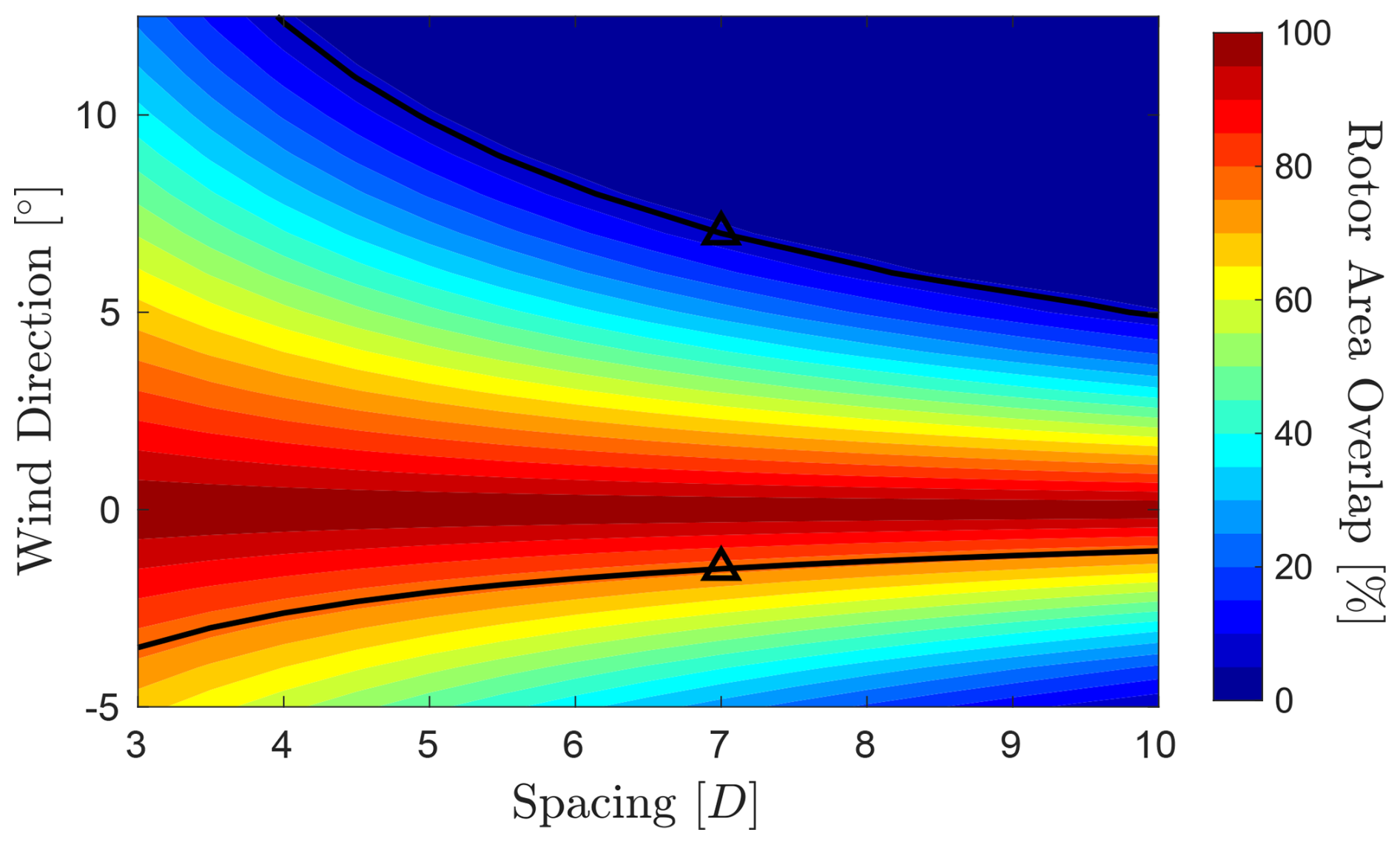
Figure 11 Percentage overlap of two aligned row turbine rotor areas at different spacings and for different wind directions. Markers shows the zero crossing of $\mathrm{\Delta }\stackrel{\mathrm{‾}}{P_{\text{farm}}}$, as predicted in Fig. 10B, for the spacing 7D simulated here. Lines show a constant rotor overlap percentage calculated for each marker point.

4.2 Limitations and further work

In the present work, a single yaw setpoint is applied, which remains unchanged across wind directions (as the impact of both bias and uncertainty are investigated), rather than finding optimal yaw angles for each wind direction and then applying a Gaussian convolution, thereby assuming no error in the mean, as in Rott et al. (2018). It could be the case that a “robust” yaw angle optimisation for this case would result in smaller yaw angles. This would likely decrease the peak power gain, and may not extend the beneficial range of wind directions (Rott et al., 2018). Fundamentally, the issue remains the same: the range of mean wind direction angles over which wake steering can be successfully applied stretches between, on one side, a small opposing angle, beyond which the yaw control acts to steer the wakes into the subsequent turbines rather than away from them; on the other side is an angle large enough to have relatively minimal wake interaction anyway, and hence the power losses incurred by yawing are larger than any possible benefit of wake steering. Then, any wind direction uncertainty will act to shrink this range further.

One limitation of both the current work and others considering the impact of wind direction uncertainty is exactly what type of uncertainty is simulated and how, compared to what occurs in the real atmosphere. It is well reported that short-term wind direction variability can be modelled with a Gaussian distribution, for statistics taken over 5 or 10 min periods (Gaumond et al., 2014), and that this is a more significant contributor to the total uncertainty than yaw position uncertainty (Quick et al., 2020). Yaw position uncertainty applied to each turbine individually would result in all turbines having small random offsets relative to the local wind direction, whereas this work assumes the turbines exactly face the incoming wind direction, and the bias is introduced e.g. through the wind farm controller assuming a different direction to what is locally present. This therefore represents a best case scenario, particularly regarding short-time variability, as in reality the turbines would not be exactly aligned with the wind direction.

Perhaps the biggest limitation of the results is applying a Gaussian convolution across a range of wind directions in order to extrapolate the impact of wind direction uncertainty. This relates firstly to atmospheric stability: in reality, a higher measured wind direction uncertainty may be indicative of more unstable conditions and higher turbulence intensity. This would therefore lead to improved baseline wake recovery and hence may make wake steering unfavourable regardless. However, the maximum chosen value of σ_WD = 4.5° is representative of measured values during wake steering experiments, therefore is likely to be reasonable as an upper bound to consider (Simley et al., 2020, 2021). Second, the Gaussian convolution approach simulates short-term (10 min) variability, and therefore a single fluctuation of the inflow wind direction is unlikely to have a length scale equivalent to the downstream farm extent. As a result, representing the effect of that fluctuation by rotating the entire wind farm coordinates by a certain value is perhaps an overestimate of the impact. This is emphasised by the additional gains achieved by yawing three turbines instead of only one, despite the very high local wind direction variability seen in the turbine row (e.g. it is still possible to achieve a gain from wake steering under a very high local inflow uncertainty). In the scenario studied here, with a spacing of 7D and diameter of 284 m, the flow-through time of the turbine row is 650 s at freestream velocity or 930 s assuming a wake velocity of 0.7U₀, greater than the 600 s time period length used to define σ_WD. Therefore, estimation of the impact of wind direction uncertainty greater than the inherent 2.3° may represent an upper bound. However, this does not apply to the impact of bias, and additionally the beneficial impact of assuming perfect relative alignment of the turbines may counteract any overestimation of the detrimental impact of wind direction uncertainty.

Other possible limitations inevitably stem from the single wind farm configuration and atmospheric boundary layer inflow that are utilised. As LES are computationally expensive, care was taken in the study design to create a fair and reasonable setup that allowed the impact of wind direction uncertainty to be investigated in a flow scenario where wake steering was likely to be beneficial. Therefore, the fact that high sensitivity to wind direction is shown even in this favourable flow scenario further highlights the need to improve both models and measurements, and the caution required when applying yaw control to real wind farms. Atmospheric stability is a key determinant of wake behaviour, due to driving the ambient turbulence intensity, shear and veer. Therefore, different stability conditions would result in different wake recovery and wind farm performance to that seen here, and hence could result in a narrowing of the range of mean wind directions where wake steering is beneficial or mean that wake steering is not beneficial at all. Different wind farm layouts also require additional considerations. For example, large wind farms with close lateral spacing may have a different dependency on mean inflow wind direction, as larger offset angles lead to wake interactions between neighbouring rows rather than all turbines experiencing the freestream inflow. However, the overall conclusions of this work – that wake steering is highly sensitive to wind direction uncertainty and small offsets in mean wind direction – are still relevant to all of these scenarios. Finally, the simulations are performed with IEA22MW turbines, but the results are expected to apply across most modern-sized wind turbines. The inflow shown in Fig. 1 exhibits a near-logarithmic velocity profile and the wind direction change with height is constant below the capping inversion. Wind turbine wake behaviour scales consistently with wind turbine size for comparable inflow conditions across the rotor disc (van der Laan et al., 2020).

As this work has shown that the potential gains from wake steering are sensitive to bias and uncertainty in wind direction, the obvious next question is: are there other wind farm control strategies that would perform better? Approaches such as derating (Annoni et al., 2016) or helix control (Frederik et al., 2020) act to reduce the wake deficit rather than redirect the wake and therefore could be more robust. Recent work by Baricchio et al. (2025) combining static yaw and the helix approach in control optimisation using engineering wake models suggests that the helix is indeed more robust to wind direction uncertainty; however, further investigation using higher fidelity models could be valuable. The impact of stable and unstable atmospheric conditions on robustness to uncertainty and bias could be investigated by using a diurnal cycle, as in Hodgson et al. (2025a). Further work could also clarify the impact of using clockwise yaw angles rather than anticlockwise, as although they are known to be less beneficial, their use is often not penalised in engineering models. Considering the sensitivity seen here even for anticlockwise yaw angles, it could be that there are almost no scenarios in which clockwise yaw is beneficial when taking into account realistic wind direction uncertainty.

5 Conclusions

This work investigates the impact of bias and uncertainty in inflow wind direction on wake steering wind farm flow control by conducting LES on a row of four turbines with 7D spacing, using a conventionally neutral boundary layer inflow. Coordinate rotations are applied to the wind farm to simulate inflow wind directions of $[-\mathrm{5},-\mathrm{3},\mathrm{0},\mathrm{3},\mathrm{5},\mathrm{8}]\mathit{°}$. Three yaw configurations are compared: a baseline with no yaw, the first turbine yawed anticlockwise by 20° and the first three turbines yawed anticlockwise by 20°. When studying both flow and power output, the impact of veer interaction is significant, leading to a 8 % difference in power output between unyawed configurations for both pairs WD = $[-\mathrm{3},\mathrm{3}]\mathit{°}$ and WD = $[-\mathrm{5},\mathrm{5}]\mathit{°}$. The wake of the first turbine exhibits a skewed and/or curled mean wake shape due to veer and/or yaw, but after the second turbine this becomes much less apparent in aligned row cases, as the wake properties begin to dominate the flow. The local inflow wind direction standard deviation significantly increases between the leading turbine and those that experience waked inflows, highlighting the increased uncertainty that is present in deep wake cases. When studying the damage equivalent loads of flapwise blade root bending moments, partial wake cases show the highest loading, and applying wake steering causes load reductions for these cases.

For the wind direction uncertainty inherent in the LES (σ_WD = 2.3°), the peak wind farm power change due to yawing occurs at a mean wind direction of 2°, with increases of 23 % and 7.5 % for the three-turbine and one-turbine yaw configurations, respectively. Positive power changes occur over a range of mean wind directions $\in [-\mathrm{1.5}\mathit{°},\mathrm{7.0}\mathit{°}]$. The peak gain of 23 % is roughly equivalent to the power increase caused by a 2–3° change in mean wind direction in the unyawed baseline. When investigating a wind direction uncertainty of σ_WD = 4.5° by applying a Gaussian convolution to the results from different wind directions, the peak power gains reduce to 7.5 % over a range of $\in [-\mathrm{1}\mathit{°},\mathrm{7}\mathit{°}]$, and 2.0 %, and over a range of ∈ [0.5°, 7°], respectively. Both the significant decrease in expected power peak with increased wind direction uncertainty, and the relatively small range of inflow wind directions over which positive power changes are predicted (regardless of uncertainty), demonstrate the challenges with applying wake steering operationally. Even if the mean inflow direction is precisely known, this study shows that it arguably might still not be worthwhile to apply wake steering when the uncertainty is high. And, conversely, if the wind direction standard deviation could be accurately measured and known to be low, then even a ± 3–4° bias in the mean wind direction measurement (which could occur e.g. due to measurement error or by assuming a single value across an entire large wind farm) is enough to remove the predicted gains for this wind farm spacing (7D). Therefore, it is important that robust and accurate wind direction measurements are available locally at each turbine to help reduce the impact of mean wind direction bias. It may also be advisable to specify a minimum range of wind directions for predicted gains to occur over before considering wake steering, such that expected levels of uncertainty cannot accidentally lead to losses.