Fast response methods for aero-elastic floating wind turbine design

Fast response calculations in the frequency domain are valuable during the initial design of floating wind turbines, where many design variants must be evaluated. A direct frequency-domain treatment of aero-elastic rotor loads is typically infeasible due to the azimuthal time dependence of the system matrices. To overcome this limitation, we introduce a perturbation-based formulation inspired by Hill's method, which reformulates the response equations into separate orders involving constant system matrices derived via Fourier decomposition. This enables accurate and efficient response computation using the fast Fourier transform (FFT). For comparison, a Laplace-based perturbation method is also developed using the Laplace transform instead of the Fourier transform. To evaluate the novel fast response methods, we develop an azimuthally periodic and fully linearized model of a floating wind turbine. The response to various load cases is computed under different inflow and floater motion conditions. The proposed Fourier-based fast response method achieves high accuracy, with peak and standard deviation errors of 2 % and 3.5 %, respectively, while reducing computation time to 2.5 s for a 4096 s simulation – significantly faster than linear (45 s) and time-domain (90 s) models. Through detailed comparison, we find that one of our approaches, the so-called single perturbation method, offers an effective trade-off between accuracy and speed, making it suitable for design and optimization studies.

1 Introduction

During the concept development and optimization phase of floating wind turbine design, methods based on linearized models are useful to quickly calculate aerodynamic and hydrodynamic response from pre-computed rotor loads. As a wide range of aerodynamic and hydrodynamic load cases are necessary to be tested, the development of a frequency-domain solver is a solution in providing computationally fast responses.

An example of a frequency-domain solver that leverages pre-computed rotor loads and a pre-computed radiation hydrodynamic damping is the QuLAF (Quick Load Analysis of Floating wind turbines) model. The QuLAF model was introduced by Pegalajar-Jurado et al. (2018) and its performance was further studied by Madsen et al. (2019). It was designed to solve the equations of motion (EOMs) in the frequency domain to increase the simulation speed and to facilitate the consideration of frequency-dependent effects, such as added hydrodynamic mass or radiation damping. Its efficiency relies on the fast Fourier transform (FFT) solution of a 4 degrees of freedom (DOFs) model that accounts for the floater surge, heave, and pitch, and the first tower mode's modal amplitude. It considers the aerodynamic rotor loads to be concentrated as a thrust and moment located at the rotor hub height position and includes the surge, heave, and pitch forcing at the floater basis. QuLAF's features have been proven to be useful, notably for the geometric optimization of a TetraSpar floater (Pollini et al., 2023) for a 15 MW wind turbine. Similarly, NREL's Response Amplitudes of Floating Turbines (RAFT) model (Hall et al., 2022) was developed to solve the dynamic response in the frequency domain using the EOMs (Hall et al., 2023) and has also been applied for control, optimization, and mooring analysis purposes (Hall et al., 2022; Zalkind and Bortolotti, 2024; Lozon et al., 2024). Another related fast solver is the Simplified Low-Order Wind turbine (SLOW) model (Schlipf et al., 2013), which was initially developed for non-linear model predictive control in floating wind energy applications, and has since been extended for control and optimization purposes (Lemmer et al., 2017, 2020a, b, 2021). Recent efforts from the Norwegian University of Science and Technology (NTNU) have also focused on applying frequency-domain solvers for floater and mooring designs (Abdelmoteleb and Bachynski-Polić, 2024, 2025).

These fast response solvers are beneficial in the preliminary design phase of floating wind turbines because FFT-based linearized models substantially reduce computational cost compared to a time-domain model (TDM) or linear model (LM). In terms of hydrodynamic loads, these typically include wave-induced forces, added mass, hydrostatic effects, and radiation damping, which can be accounted for in the system matrices. As mentioned, the aerodynamic rotor loads, however, are usually pre-calculated with a non-moving nacelle and parameterized aerodynamic damping. In this decomposition, the rotor loads are due to the turbulent inflow variation, while the aerodynamic damping arises from the relative motion between the structure and the airflow. Since these effects are naturally embedded in full aero-elastic models, the extraction of linearized forcing and damping is possible through linearization. Due to the azimuthal dependence of blade positions, however, the resulting system matrix is not constant in time, and transformation to the frequency domain and solution by FFT are not directly possible.

To address this limitation, the present study introduces novel fast response methods for a blade-resolved LM that are executed with the FFT algorithm as in the QuLAF code. For comparison with Fourier-based methods, we implement a technique that uses the inverse Laplace transform to convert the solution from the s domain to the time domain. The novelty of this study lies in the development of fast response methods based on the separation of time-varying elements of the system matrices and corrections within a state-space formulation, which can be expressed in either the frequency or Laplace domain.

Building on this foundation, the present work extends frequency- and Laplace-domain methodologies to floating wind energy with a focus on blade aerodynamic loads rather than floater hydrodynamic and mooring loads. In our model, we explicitly account for blade-dependent rotor loads in both the frequency and Laplace domain, rather than reducing them to thrust and moment at the rotor hub, as done in existing models such as QuLAF, RAFT, and SLOW. While previous studies modelled the EOM in state-space form without considering azimuthal blade load effects, our formulation includes these effects directly. Linearizing motion-coupled aerodynamic forces remains challenging because of the blades' passage through a disturbed inflow, leading to time-variant azimuthal dependencies in the system matrices. To enable the assembly of a constant system transfer function, one needs to get around the azimuthal dependence of the system matrix.

The proposed fast response methods draw inspiration from Hill's method (Hill, 1886), which employs harmonic decomposition to convert a periodic system into a linear time-invariant (LTI) one – a process also related to Floquet's theory (Floquet, 1883). Our previous work (Pamfil et al., 2025) has shown that Hill's method produces stability analysis results consistent with Floquet's theory and Coleman's (Coleman and Feingold, 1958) transformation, while avoiding the latter's limitations for two-bladed rotors or cases with wind shear and gravity effects. The fast response methods that we developed are particularly relevant for linearized models in which the Coleman transform does not yield time-invariant system matrices and where the accurate resolution of rotor loads is required. The transformation is designed to eliminate only the first-harmonic (1P) periodicity related to the rotational speed and does not remove higher-order harmonic contributions (Pamfil, 2025). This occurs, for instance, in two-bladed turbines, for which the transformation does not produce an azimuthally time-invariant (constant) mass matrix, as well as in three-bladed turbines operating under strong shear conditions, where significant higher harmonic content persists in the system. Consequently, our fast response methods enable the efficient evaluation of rotor loads in situations where residual periodicity remains in a Coleman transformed system. For such periodic systems, eigenmode analysis can be conducted by Hill's method, which uses a truncated Fourier series to decompose the system matrix into a harmonic summation of constant terms. The reliability and accuracy of this decomposition have been further verified by Hansen (2016) and Skjoldan (2009). Consequently, we exploit this harmonic decomposition to enable fast response calculations based on the FFT algorithm (Cooley and Tukey, 1965) and to develop a Laplace-based method relying on the inverse of the Laplace transform.

The FFT algorithm (Cooley and Tukey, 1965) ensures computational efficiency in the frequency domain while the Laplace transform provides a pathway for response analysis through transfer functions represented in the s domain. Although Laplace-domain computations require the inverse transformation to obtain time-domain results – often a computational bottleneck – various numerical inversion algorithms, such as Talbot's method (Talbot, 1979), Stehfest's algorithm (Stehfest, 1970), and the de Hoog continued fraction method (de Hoog et al., 1982), offer accurate solutions. In this study, MATLAB's symbolic inverse Laplace function (ilaplace) is used for convenience.

The fast response methods in this paper are verified using a simplified four-DOF floating wind turbine model, incorporating floater pitch motion and blade flapwise deflection (first mode only), as well as dynamic stall and gravity effects. The rotor speed is assumed constant, and pitch control and tower deflection are neglected to reduce complexity. Other modelling assumptions relate to hydrodynamic loading on the floater, dynamic stall, and the number of blade sections and modes used in rotor load computations. This simplified four-DOF model was chosen to enable efficient validation while retaining the dominant coupled aero-hydro-elastic effects. These assumptions do introduce certain limitations with respect to the behaviour of a full-scale floating wind turbine. In particular, neglecting tower flexibility removes the dynamics associated with tower bending and its coupling to the platform motion, while assuming constant rotor speed and omitting blade pitch control disregards control-induced coupling effects and load mitigation mechanisms. Yet, the tower flexibility can readily be incorporated by following the same approach as in the QuLAF model (Pegalajar-Jurado et al., 2018). Moreover, the inclusion of varying rotor speed and control is a natural extension of both the stability method of Pamfil et al. (2025) and has been described in Pamfil (2025). However, the included dynamics capture the key degrees of freedom relevant to demonstrating the proposed fast response methods. Therefore, despite its simplicity, the model remains suitable for demonstrating the effectiveness of the fast response methods that we developed and for identifying trends that are expected to persist in more complete models.

Multiple load cases are simulated, including steady, sheared, and turbulent inflow, and harmonic or stochastic floater pitch excitation. The accuracy for the fast response calculation variants is analysed for a given duration against benchmark results of the original LM. Metrics include the exceedance probability results and the standard deviation relative error (SDRE) with respect to the LM and CPU time. Results demonstrate that fast response methods achieve a good trade-off between speed and accuracy. With limited loss of accuracy, they can potentially accelerate the state-of-the-art TDMs such as HAWC2, OpenFAST, SIMA, and Bladed, making them promising tools for the early-stage design and optimization of floating offshore wind turbines (FOWTs).

2 Model description

As illustrated in Fig. 1, the floating wind turbine model considered operates at a constant rotational speed Ω and has 4 structural DOFs, being the flapwise deflection of the three blades, denoted by a_l; and the floater's pitch angular motion, represented by ξ₅. Floater surge motion was not included in order to reduce the model's complexity and to focus on the dominant coupled pitch–blade dynamics relevant to the proposed fast response methods. In other words, the model is intended to provide a minimal representation of the coupled floater–blade response. Including the floater surge would introduce additional coupling effects and wake–platform interactions. This would require the consideration of a dynamic wake model with time-varying induction factors in the directions normal and tangential to the rotor plane, which is beyond the scope of the current model. The paper aims to develop an analytical model that could combine platform surge motion with dynamic inflow effects in future extensions, while the present work focuses on establishing and validating the core formulation. Nonetheless, among the floater surge and pitch DOFs, pitch is the most dynamically significant for floating wind turbines, as it typically exhibits the highest natural frequency and is the mode in which control-induced instabilities may arise under above-rated wind speed conditions (Larsen and Hanson, 2007). Moreover, there is a hydrodynamic forcing moment M_F exerted on the floater base, which represents wave forcing. The dynamic rotor loads for each lth blade are applied in the rotor out-of-plane direction (along the ${\widehat{y}}^{\prime }$ axis), which coincides with the blade deflection u_l(r,t). These loads arise from a concentrated aerodynamic blade force F_l,aero applied at a reference location d from the hub, as well as from a constant velocity V₀ with the fluctuation ΔV_0,l generated by a sheared and turbulent inflow. The blade aerodynamic loads and the contributions to wind velocity from the constant velocity V₀, turbulent fluctuation $\mathrm{\Delta }{V}_{\mathrm{0},l,\mathrm{turb}}$, and sheared inflow $\mathrm{\Delta }{V}_{\mathrm{0},l,\mathrm{shear}}$ are illustrated in Fig. 1. More details about the considered floating wind turbine model can be found in the author's previous related work (Pamfil et al., 2025). In this paper, we extend the floating wind turbine model to include wind loads acting on blade elements of mass m(r), wave loads applied at the floater base, and gravitational loads exerted on the blade elements as well as on the hub and nacelle of cumulative mass M.

The floating wind turbine model (Pamfil et al., 2025) also includes Øye's dynamic stall model (Øye, 1991), through 3 additional aerodynamic DOFs. The blade deflection is approximated using a modal approach, where only the blade first flapwise mode (1f) contribution is taken into account. The reason why the blade deflection approximation is computed using only the blade first flapwise mode is in order to alleviate the model's number of DOFs and thus simplify it. The structural properties of the floating wind turbine, such as the blade first flapwise mode's characteristics (natural frequency ω_1f, mode shape ϕ_1f, and modal mass), blade length L_b, mass per unit length m(r), rotor hub height H, and combined mass M for the hub and nacelle, are all based on the DTU 10 MW reference wind turbine (Bak et al., 2013). The floater pitching moment coefficient $K_{{\mathit{\xi }}_{\mathrm{5}}}$ describes the component of the water plane stiffness matrix due to hydrostatic effects. The value of $K_{{\mathit{\xi }}_{\mathrm{5}}}$ was chosen to achieve a floater pitch period of 28.57 s and thus a frequency of $f_{{\mathit{\xi }}_{\mathrm{5}}}=\mathrm{0.035}\mathrm{Hz}$ (Pamfil et al., 2025).

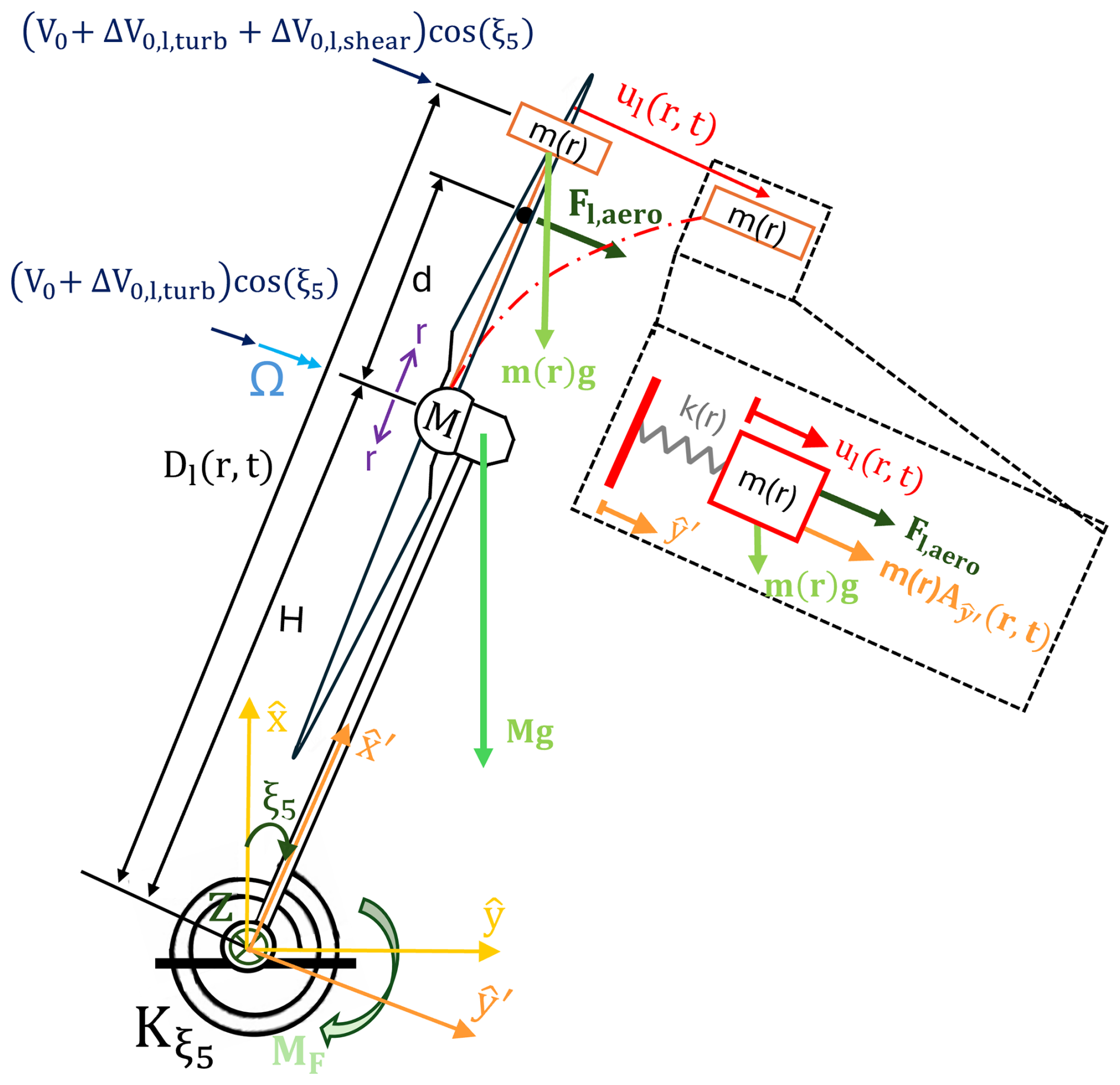
Figure 1 Floating wind turbine model where blade properties and parameters vary in the radial direction r and with blade index l. This includes the blade deflection u_l(r,t) and the distance of a blade element mass m(r) from the floater base being D_l(r,t).

The distance d measured from the hub marks a reference radial position r=d along the blade, at 70 % of the blade's length (d=0.7L_b), where the aerodynamic load on each blade F_l,aero is calculated. F_l,aero is indicative of the load distribution along the entire blade.

Finally, it should be emphasized that this floating wind turbine model serves solely as a representative case study to illustrate the proposed fast response methods. As previously noted, the model makes simplifying assumptions regarding the dynamic stall, number of blade sections and modes in rotor load calculations, and hydrodynamic loading on the floater. Despite these simplifications, it provides a basis for demonstrating the fast response methods, with future work aimed at applying it within a fully detailed modelling framework.

2.1 Equations of motion

For completeness, we provide a summary of the derivation of EOMs that we have already elaborated on in previous work (Pamfil et al., 2025). To this end, we introduce the time-varying azimuthal angular position Ψ_l(t) of a blade l, which is defined as ${\mathrm{\Psi }}_l\left(t\right)=\frac{\mathrm{2}\mathit{\pi }}{N_{\mathrm{b}}}\left(l-\mathrm{1}\right)+\mathrm{\Omega }t$ and where N_b=3 is the rotor's number of blades and Ω is its constant rotational speed.

For a non-deformed blade, the time-varying distance D_l(r,t) of a blade element with mass m(r) along the ${\widehat{x}}^{\prime }$ axis is calculated relative to the floater base position. It is also impacted by the radial position r from the hub, yielding $D_l(r,t)=H+r\cos {\mathrm{\Psi }}_l\left(t\right)$. For a deformed blade case, the local blade deflection u_l(r,t) is computed as $u_l(r,t)={\mathit{\varphi }}_{\mathrm{1}\mathrm{f}}\left(r\right)a_l\left(t\right)$, where only the first flapwise (1f) mode shape ϕ_1f(r) with amplitude a_l(t) is taken into consideration.

Subsequently, given a blade element's distance D_l(r,t) from the floater basis and its deflection u_l(r,t), its position ${\widehat{D}}_l(r,t)$ is tracked as ${\widehat{D}}_l(r,t)=D_l(r,t){\widehat{x}}^{\prime }\left(t\right)+u_l(r,t){\widehat{y}}^{\prime }\left(t\right)$, in the pitching coordinate system $({\widehat{x}}^{\prime },{\widehat{y}}^{\prime })$. Figure 1 shows that the unit vectors ${\widehat{x}}^{\prime }$ and ${\widehat{y}}^{\prime }$ can be expressed in terms of the global fixed coordinates $\widehat{x}$ and $\widehat{y}$, as ${\widehat{x}}^{\prime }=\cos \left({\mathit{\xi }}_{\mathrm{5}}\right)\widehat{x}+\sin \left({\mathit{\xi }}_{\mathrm{5}}\right)\widehat{y}$ and ${\widehat{y}}^{\prime }=-\sin \left({\mathit{\xi }}_{\mathrm{5}}\right)\widehat{x}+\cos \left({\mathit{\xi }}_{\mathrm{5}}\right)\widehat{y}$. This allows us to deduce the following time derivatives of ${\dot{\widehat{x}}}^{\prime }={\dot{\mathit{\xi }}}_{\mathrm{5}}{\widehat{y}}^{\prime }$ and ${\dot{\widehat{y}}}^{\prime }=-{\dot{\mathit{\xi }}}_{\mathrm{5}}{\widehat{x}}^{\prime }$. These two relations between the pitching coordinates ${\widehat{x}}^{\prime }$ and ${\widehat{y}}^{\prime }$ are valid irrespective of the amplitude of the floater pitch angle ξ₅. As previously demonstrated (Pamfil et al., 2025), these time derivatives are then used to lay out the kinematic equations for velocity ${\widehat{V}}_l(r,t)$, acceleration ${\widehat{A}}_l(r,t)=A_{{\widehat{x}}^{\prime },l}{\widehat{x}}^{\prime }+A_{{\widehat{y}}^{\prime },l}{\widehat{y}}^{\prime }$, and the rate of change of angular momentum p_l(r,t) around the axis $\widehat{z}={\widehat{x}}^{\prime }\times {\widehat{y}}^{\prime }$. The resulting linearized rate of change of angular momentum $p_{l,\mathrm{lin}}(r,t)$ can be described as

$$\begin{array}{}\text{(1)}& \begin{array}{rl}{p}_l(r,t)& \approx p_{l,\mathrm{lin}}(r,t)=m\left(r\right)\left(D_l^{\mathrm{2}}\right(r,t){\ddot{\mathit{\xi }}}_{\mathrm{5}}\\ & +\mathrm{2}{D}_l(r,t){\dot{D}}_l(r,t){\dot{\mathit{\xi }}}_{\mathrm{5}}+D_l(r,t){\ddot{u}}_l(r,t)\\ & -{\ddot{D}}_l(r,t)u_l(r,t)).\end{array}\end{array}$$

Moving forward, the translational and pitching motion equations can be derived, along with the resulting EOM. To derive the EOM, we first establish the pitching motion equation for moments about the $\widehat{z}$ axis as

$$\begin{array}{}\text{(2)}& \begin{array}{rl}& \widehat{z}:M{H}^{\mathrm{2}}{\ddot{\mathit{\xi }}}_{\mathrm{5}}\mathit{\delta }{\mathit{\xi }}_{\mathrm{5}}+K_{{\mathit{\xi }}_{\mathrm{5}}}{\mathit{\xi }}_{\mathrm{5}}\mathit{\delta }{\mathit{\xi }}_{\mathrm{5}}+MgH\sin {\mathit{\xi }}_{\mathrm{5}}\mathit{\delta }{\mathit{\xi }}_{\mathrm{5}}+\\ & \sum _{l=\mathrm{1}}^{N_{\mathrm{b}}}\left(\underset{\mathrm{0}}{\overset{L_{\mathrm{b}}}{\int }}\left(p_{l,\mathrm{lin}}(r,t)+m\left(r\right)g{D}_l(r,t)\sin {\mathit{\xi }}_{\mathrm{5}}\right)\mathrm{d}r\mathit{\delta }{\mathit{\xi }}_{\mathrm{5}}\right)\\ & =M_{\mathrm{F}}\mathit{\delta }{\mathit{\xi }}_{\mathrm{5}}+\underset{{\mathrm{M}}_{\mathrm{aero}}}{\underbrace{\left(\sum _{l=\mathrm{1}}^{N_{\mathrm{b}}}{D}_l(d,t)F_{l,\mathrm{aero}}\left(t\right)\right)}}\mathit{\delta }{\mathit{\xi }}_{\mathrm{5}},\end{array}\end{array}$$

through the conservation of angular momentum for a virtual pitch angle δξ₅. In Eq. (2), there is an internal angular momentum forcing component that considers the gravitational load contribution of the nacelle and hub having a cumulative mass M. The other gravitational angular momentum load contribution is accounted for by integrating the distributed mass m(r) along the blade span with a moment arm D_l(r,t). The external forcing arises from the applied floater pitch moment M_F and the induced aerodynamic moment M_aero, which is generated by the aerodynamic loads F_l,aero acting with the same moment arm D_l(r,t).

In addition, the equation of translational motion along the ${\widehat{y}}^{\prime }$ axis for each blade is obtained as

$$\begin{array}{}\text{(3)}& \begin{array}{rl}& {\widehat{y}}^{\prime }:\underset{\mathrm{0}}{\overset{L_{\mathrm{b}}}{\int }}\left(\underset{f_{{\widehat{y}}^{\prime },l}(r,t)}{\underbrace{m\left(r\right)A_{{\widehat{y}}^{\prime },l}(r,t)}}+m\left(r\right)g\sin {\mathit{\xi }}_{\mathrm{5}}\right)\mathit{\delta }{a}_l{\mathit{\varphi }}_{\mathrm{1}\mathrm{f}}\left(r\right)\mathrm{d}r+\\ & \underset{K_{{\mathrm{a}}_l}{a}_l\mathit{\delta }{a}_l}{\underbrace{\underset{\mathrm{0}}{\overset{L_{\mathrm{b}}}{\int }}k\left(r\right)a_l\left(t\right){\mathit{\varphi }}_{\mathrm{1}\mathrm{f}}\left(r\right)\left(\mathit{\delta }{a}_l{\mathit{\varphi }}_{\mathrm{1}\mathrm{f}}\left(r\right)\right)\mathrm{d}r}}\\ & =\underset{G{F}_{{\mathrm{a}}_l}}{\underbrace{F_{l,\mathrm{aero}}\left(t\right){\mathit{\varphi }}_{\mathrm{1}\mathrm{f}}\left(d\right)}}\mathit{\delta }{a}_l,\end{array}\end{array}$$

where the blade displacement virtual work is given by $\mathit{\delta }{u}_l(r,t)=\mathit{\delta }{a}_l\left(t\right){\mathit{\varphi }}_{\mathrm{1}\mathrm{f}}\left(r\right)$. In Eq. (3), the inertial force $f_{{\widehat{y}}^{\prime },l}(r,t)=m\left(r\right)A_{{\widehat{y}}^{\prime },l}(r,t)$ for a mass element m(r) is influenced by the linearized tangential acceleration $A_{{\widehat{y}}^{\prime },l}(r,t)$, where only linear terms are retained. Here, k(r) represents the blade sectional stiffness, defined as $k\left(r\right)=m\left(r\right){\mathit{\omega }}_{\mathrm{1}\mathrm{f}}^{\mathrm{2}}$, which is derived from the first flapwise natural frequency ω_1f, while ϕ_1f(d) represents the value of the first flapwise mode shape at r=d. The blade internal gravitational load is obtained by integrating the load component perpendicular to the rotor plane along the blade span. The external blade force considered in Eq. (3) for each lth blade is denoted as the generalized aerodynamic blade force $G{F}_{{\mathrm{a}}_l}$.

The forcing terms for both the pitching and translation motion equations are implemented in the TDM forcing vector F_T. The TDM's dynamics is described by the following EOM:

$$\begin{array}{}\text{(4)}& {\mathbf{M}}_{\mathrm{S}}\ddot{\mathit{x}}+{\mathbf{C}}_{\mathrm{S}}\dot{\mathit{x}}+{\mathbf{K}}_{\mathrm{S}}\mathit{x}={\mathit{F}}_{\mathrm{T}}.\end{array}$$

In this EOM, the vector of structural DOFs is defined as $\mathit{x}={\left[{\mathit{\xi }}_{\mathrm{5}},a_{\mathrm{1}},a_{\mathrm{2}},a_{\mathrm{3}}\right]}^T$, where ξ₅ denotes the floater pitch angle and a₁, a₂, and a₃ represent the blade deflection amplitudes of blades 1, 2, and 3, respectively. Equation (4) also includes the structural (index “S”) mass M_S, damping C_S, and stiffness K_S matrices. The structural mass and damping matrices are taken from the model developed in our earlier work on floating wind turbine stability analysis (Pamfil et al., 2025) which gives:

$$\begin{array}{}\text{(5)}& \begin{array}{rl}& {\mathbf{M}}_{\mathrm{S}}=\left[\begin{array}{cccc}M{H}^{\mathrm{2}}& \mathrm{0}& \mathrm{0}& \mathrm{0}\\ \mathrm{0}& \mathrm{0}& \mathrm{0}& \mathrm{0}\\ \mathrm{0}& \mathrm{0}& \mathrm{0}& \mathrm{0}\\ \mathrm{0}& \mathrm{0}& \mathrm{0}& \mathrm{0}\end{array}\right]+\underset{\mathrm{0}}{\overset{L_{\mathrm{b}}}{\int }}m\left(r\right){\mathbf{M}}_{\mathrm{S},\mathrm{b}}\left(r\right)\mathrm{d}r\\ & {\mathbf{M}}_{\mathrm{S},\mathrm{b}}=\left[\begin{array}{cccc}{\sum }_{l=\mathrm{1}}^{\mathrm{3}}{D}_l^{\mathrm{2}}(r,t)& D_{\mathrm{1}}(r,t){\mathit{\varphi }}_{\mathrm{1}\mathrm{f}}\left(r\right)& D_{\mathrm{2}}(r,t){\mathit{\varphi }}_{\mathrm{1}\mathrm{f}}\left(r\right)& D_{\mathrm{3}}(r,t){\mathit{\varphi }}_{\mathrm{1}\mathrm{f}}\left(r\right)\\ D_{\mathrm{1}}(r,t){\mathit{\varphi }}_{\mathrm{1}\mathrm{f}}\left(r\right)& {\mathit{\varphi }}_{\mathrm{1}\mathrm{f}}^{\mathrm{2}}\left(r\right)& \mathrm{0}& \mathrm{0}\\ D_{\mathrm{2}}(r,t){\mathit{\varphi }}_{\mathrm{1}\mathrm{f}}\left(r\right)& \mathrm{0}& {\mathit{\varphi }}_{\mathrm{1}\mathrm{f}}^{\mathrm{2}}\left(r\right)& \mathrm{0}\\ D_{\mathrm{3}}(r,t){\mathit{\varphi }}_{\mathrm{1}\mathrm{f}}\left(r\right)& \mathrm{0}& \mathrm{0}& {\mathit{\varphi }}_{\mathrm{1}\mathrm{f}}^{\mathrm{2}}\left(r\right)\end{array}\right],\end{array}\end{array}$$

and

$$\begin{array}{}\text{(6)}& \begin{array}{rl}& {\mathbf{C}}_{\mathrm{S}}=\left[\begin{array}{cccc}{\mathit{\mu }}_{{\mathit{\xi }}_{\mathrm{5}}}{K}_{{\mathit{\xi }}_{\mathrm{5}}}& \mathrm{0}& \mathrm{0}& \mathrm{0}\\ \mathrm{0}& \mathrm{0}& \mathrm{0}& \mathrm{0}\\ \mathrm{0}& \mathrm{0}& \mathrm{0}& \mathrm{0}\\ \mathrm{0}& \mathrm{0}& \mathrm{0}& \mathrm{0}\end{array}\right]+\underset{\mathrm{0}}{\overset{L_{\mathrm{b}}}{\int }}m\left(r\right){\mathbf{C}}_{\mathrm{S},\mathrm{b}}\left(r\right)\mathrm{d}r\\ & {\mathbf{C}}_{\mathrm{S},\mathrm{b}}=\left[\begin{array}{cccc}{\sum }_{l=\mathrm{1}}^{\mathrm{3}}\mathrm{2}{D}_l(r,t){\dot{D}}_l(r,t)& \mathrm{0}& \mathrm{0}& \mathrm{0}\\ \mathrm{2}{\dot{D}}_{\mathrm{1}}(r,t){\mathit{\varphi }}_{\mathrm{1}\mathrm{f}}\left(r\right)& {\mathit{\mu }}_{{\mathrm{a}}_{\mathrm{1}}}{\mathit{\omega }}_{\mathrm{1}\mathrm{f}}^{\mathrm{2}}{\mathit{\varphi }}_{\mathrm{1}\mathrm{f}}^{\mathrm{2}}\left(r\right)& \mathrm{0}& \mathrm{0}\\ \mathrm{2}{\dot{D}}_{\mathrm{2}}(r,t){\mathit{\varphi }}_{\mathrm{1}\mathrm{f}}\left(r\right)& \mathrm{0}& {\mathit{\mu }}_{{\mathrm{a}}_{\mathrm{2}}}{\mathit{\omega }}_{\mathrm{1}\mathrm{f}}^{\mathrm{2}}{\mathit{\varphi }}_{\mathrm{1}\mathrm{f}}^{\mathrm{2}}\left(r\right)& \mathrm{0}\\ \mathrm{2}{\dot{D}}_{\mathrm{3}}(r,t){\mathit{\varphi }}_{\mathrm{1}\mathrm{f}}\left(r\right)& \mathrm{0}& \mathrm{0}& {\mathit{\mu }}_{{\mathrm{a}}_{\mathrm{3}}}{\mathit{\omega }}_{\mathrm{1}\mathrm{f}}^{\mathrm{2}}{\mathit{\varphi }}_{\mathrm{1}\mathrm{f}}^{\mathrm{2}}\left(r\right)\end{array}\right].\end{array}\end{array}$$

However, the stiffness matrix now includes gravitational terms, rendering it as follows:

$$\begin{array}{}\text{(7)}& \begin{array}{rl}& {\mathbf{K}}_{\mathrm{S}}=\left[\begin{array}{cccc}{K}_{{\mathit{\xi }}_{\mathrm{5}}}+MgH& \mathrm{0}& \mathrm{0}& \mathrm{0}\\ \mathrm{0}& \mathrm{0}& \mathrm{0}& \mathrm{0}\\ \mathrm{0}& \mathrm{0}& \mathrm{0}& \mathrm{0}\\ \mathrm{0}& \mathrm{0}& \mathrm{0}& \mathrm{0}\end{array}\right]+\underset{\mathrm{0}}{\overset{L_{\mathrm{b}}}{\int }}m\left(r\right){\mathbf{K}}_{\mathrm{S},\mathrm{b}}\left(r\right)\mathrm{d}r\\ & {\mathbf{K}}_{\mathrm{S},\mathrm{b}}=\left[\begin{array}{cccc}{\mathrm{\Sigma }}_{l=\mathrm{1}}^{\mathrm{3}}g{D}_l(r,t)& -{\ddot{D}}_{\mathrm{1}}(r,t){\mathit{\varphi }}_{\mathrm{1}\mathrm{f}}\left(r\right)& -{\ddot{D}}_{\mathrm{2}}(r,t){\mathit{\varphi }}_{\mathrm{1}\mathrm{f}}\left(r\right)& -{\ddot{D}}_{\mathrm{3}}(r,t){\mathit{\varphi }}_{\mathrm{1}\mathrm{f}}\left(r\right)\\ g{\mathit{\varphi }}_{\mathrm{1}\mathrm{f}}\left(r\right)& {\mathit{\omega }}_{\mathrm{1}\mathrm{f}}^{\mathrm{2}}{\mathit{\varphi }}_{\mathrm{1}\mathrm{f}}^{\mathrm{2}}\left(r\right)& \mathrm{0}& \mathrm{0}\\ g{\mathit{\varphi }}_{\mathrm{1}\mathrm{f}}\left(r\right)& \mathrm{0}& {\mathit{\omega }}_{\mathrm{1}\mathrm{f}}^{\mathrm{2}}{\mathit{\varphi }}_{\mathrm{1}\mathrm{f}}^{\mathrm{2}}\left(r\right)& \mathrm{0}\\ g{\mathit{\varphi }}_{\mathrm{1}\mathrm{f}}\left(r\right)& \mathrm{0}& \mathrm{0}& {\mathit{\omega }}_{\mathrm{1}\mathrm{f}}^{\mathrm{2}}{\mathit{\varphi }}_{\mathrm{1}\mathrm{f}}^{\mathrm{2}}\left(r\right)\end{array}\right].\end{array}\end{array}$$

The gravity terms in the structural matrix K_S consider the small floater tilt assumption, such that sin ξ₅≈ξ₅. Inspired from the Rayleigh damping approach, we have chosen the structural contribution of the structural damping matrix C_S to be expressed as μK_S, where μ is a scaling factor applied to the structural stiffness matrix. In this expression, only the diagonal elements of the structural stiffness matrix K_S, which are not affected by gravitational effects, are utilized in C_S. As for the hydrodynamic damping contribution ${\mathit{\mu }}_{{\mathit{\xi }}_{\mathrm{5}}}{K}_{{\mathit{\xi }}_{\mathrm{5}}}$ to the structural damping matrix C_S, it is included in Eq. (6). The approximation for the damping ratio ζ_k can be written as

$$\begin{array}{}\text{(8)}& {\mathit{\zeta }}_k={\displaystyle \frac{{\mathit{\delta }}_k}{\sqrt{\mathrm{4}{\mathit{\pi }}^{\mathrm{2}}+{\mathit{\delta }}_k^{\mathrm{2}}}}}\approx {\displaystyle \frac{{\mathit{\delta }}_k}{\mathrm{2}\mathit{\pi }}}\text{ and }{\mathit{\mu }}_k={\displaystyle \frac{\mathrm{2}{\mathit{\zeta }}_k}{{\mathit{\omega }}_k}},\end{array}$$

where δ_k is the logarithmic decrement for a kth degree of freedom. It is valid for sufficiently small damping ratios, which is consistent with the present application. In the floating wind turbine context, the torsional structural damping applied to the platform pitch DOF ξ₅ is used to represent the dominant hydrodynamic damping associated with the floater motion. For the TetraSpar concept, a pitch damping ratio of ${\mathit{\zeta }}_{{\mathit{\xi }}_{\mathrm{5}}}=\mathrm{3}\mathit{\%}$ with a corresponding logarithmic decrement of ${\mathit{\delta }}_{{\mathit{\xi }}_{\mathrm{5}}}=\mathrm{0.20}$ is reported by Borg et al. (2024), resulting in a damping factor of ${\mathit{\mu }}_{{\mathit{\xi }}_{\mathrm{5}}}=\mathrm{0.30}$. This value reflects the combined effect of structural and hydrodynamic damping acting on the platform pitch response. Hence, the hydrodynamic damping is lumped into an equivalent stiffness-proportional damping term for the floater pitch angle DOF. Linear potential theory (LPT) solvers, such as wave analysis MIT (WAMIT), can provide frequency-domain estimates of hydrodynamic excitation forces, radiation damping, and added mass, which can be incorporated as matrix contributions to the EOM. In our simplified framework, the frequency dependence of radiation damping is neglected and a lumped hydrodynamic damping representation is favoured instead. For the blade DOFs a_l, the damping ratio is set to a comparatively low value of ${\mathit{\zeta }}_{{\mathrm{a}}_l}=\mathrm{0.5}\mathit{\%}$ (Bak et al., 2013), with a corresponding logarithmic decrement of ${\mathit{\delta }}_{{\mathrm{a}}_l}=\mathrm{0.03}$ and damping factor of ${\mathit{\mu }}_{{\mathrm{a}}_l}=\mathrm{0.0024}$. This conveys the minor contribution of blade structural damping relative to the hydrodynamic damping of the floater.

2.2 Floater pitch moment excitation

Regarding the floater pitch moment of excitation M_F, it can be either harmonic or stochastic. The harmonic floater pitch moment M_F has an amplitude A_M and an excitation frequency Ω_M, M_F=A_Mcos (Ω_Mt), to model a regular wave forcing effect that affects the sinusoidal floater motion. The numerical value of $A_{\mathrm{M}}=\mathrm{1.212}\times {\mathrm{10}}^{\mathrm{7}}\mathrm{Nm}$ is selected to represent a realistic amplitude of the floater moment excitation for a floating wind turbine with the DTU 10 MW size and characteristics. As for the excitation frequency of ${\mathrm{\Omega }}_{\mathrm{M}}=\mathrm{0.15}\cdot \mathrm{2}\mathit{\pi }\mathrm{rad}{\mathrm{s}}^{-\mathrm{1}}$, it is also representative of a typical sea state.

However, the stochastic hydrodynamic moment M_F that is considered in this paper is extracted from simulations carried out for a water depth of h=320 m for a representative spar-buoy floater. These simulations consider the implementation of linear wave kinematics and the Morison equation to describe the hydrodynamic forces acting on the slender body through an inertia term and a non-linear viscous drag term proportional to the square of the relative velocity. However, it does not include second-order diffraction forces, mean-drift forces, slow-drift forces (difference-frequency excitations), and sum-frequency forces (higher-frequency contributions). The inclusion of these effects is possible but was left out due to the demonstration purpose of the model. The spar-buoy floater's main specifications are its submerged underwater draft ${\widehat{x}}_{\mathrm{Bot}}=-\mathrm{120}\mathrm{m}$ and its diameter D_Spar=11.2 m, which relate to the cylinder cross-sectional area $A_{\mathrm{Spar}}=\frac{\mathit{\pi }}{\mathrm{4}}{D}_{\mathrm{Spar}}^{\mathrm{2}}$. These dimensions are representative of a 10 MW spar design.

Calculating the stochastic hydrodynamic moment for a spar-buoy floater M_F=τ_hydro greatly simplifies calculations through the usage of the Morison equation. To do so, we calculate first the hydrodynamic force F_hydro per unit length and next integrate up to the still water level at $\widehat{x}=\mathrm{0}$ after multiplication with the moment arm $\widehat{x}$:

$$\begin{array}{}\text{(9)}& \begin{array}{rl}{\mathit{\tau }}_{\mathrm{hydro}}=& \underset{{\widehat{x}}_{\mathrm{Bot}}}{\overset{\mathrm{0}}{\int }}\widehat{x}{F}_{\mathrm{hydro}}d\widehat{x}\\ =& \underset{{\widehat{x}}_{\mathrm{Bot}}}{\overset{\mathrm{0}}{\int }}\widehat{x}{\mathit{\rho }}_{\mathrm{water}}{C}_{\mathrm{m}}{A}_{\mathrm{Spar}}{\dot{u}}_{\mathrm{0}}d\widehat{x}\\ & +\underset{{\widehat{x}}_{\mathrm{Bot}}}{\overset{\mathrm{0}}{\int }}{\displaystyle \frac{\mathrm{1}}{\mathrm{2}}}\widehat{x}{\mathit{\rho }}_{\mathrm{water}}{C}_{D,\mathrm{water}}{D}_{\mathrm{Spar}}{u}_{\mathrm{0}}\left|u_{\mathrm{0}}\right|d\widehat{x}.\end{array}\end{array}$$

The hydrodynamic force F_hydro is pre-calculated with no spar motion consideration. In this case, there is only a wave velocity and acceleration u₀=u_wave and ${\dot{u}}_{\mathrm{0}}={\dot{u}}_{\mathrm{wave}}$ that are perceived by the spar buoy. Due to the assumption of no spar motion, hydrodynamic damping is not explicitly modelled through the Morison force formulation. Instead, its effect is implicitly accounted for through scaling of the pitch–pitch component (1,1), namely the hydrodynamic damping term ${\mathit{\mu }}_{{\mathit{\xi }}_{\mathrm{5}}}{K}_{{\mathit{\xi }}_{\mathrm{5}}}$ in the damping matrix C_S, as discussed earlier. In Eq. (9), ρ_water denotes the water density, C_D,water is the drag coefficient, and the inertia term C_m is defined as $C_{\mathrm{m}}=\mathrm{1}+C_{\mathrm{a}}$, where C_a is the added-mass coefficient, set to C_a=1, while the remaining contribution is attributed to the Froude–Krylov force. The stochasticity in Eq. (9) stems from u_wave's spectral decomposition for a number N of wave frequency ω_wave,j samples, with a stochastic phase shift ϵ_wave,j applied:

$$\begin{array}{}\text{(10)}& \begin{array}{rl}{u}_{\mathrm{wave}}(\widehat{x},\widehat{y})=& \sum _{j=\mathrm{1}}^N{A}_{\mathrm{wave},j}{\mathit{\omega }}_{\mathrm{wave},j}{\displaystyle \frac{\cosh \left(k_{\mathrm{wave},j}\right(\widehat{x}+h\left)\right)}{\sinh \left(k_{\mathrm{wave},j}h\right)}}\\ & \cdot \cos ({\mathit{\omega }}_{\mathrm{wave},j}t+{\mathit{ϵ}}_{\mathrm{wave},j}).\end{array}\end{array}$$

In Eq. (10), A_wave,j is the wave amplitude obtained from the JONSWAP spectrum with a prescribed significant wave height H_s=1.2 m, a peak period T_p=10 s, and a peak enhancement factor of γ=3.3. The prescribed H_s and T_p values are correlated to the water depth h and to the inflow velocity V₀ for the operational state of the wind turbine. Additionally, k_wave,j is the wave number solved through the wave dispersion relation, i.e. ${\mathit{\omega }}_{\mathrm{wave},j}^{\mathrm{2}}=g{k}_{\mathrm{wave},j}\tanh \left(k_{\mathrm{wave},j}h\right)$.

2.3 Aerodynamic load

The loading vector F_T that is acting on the structure is not only influenced by the floater pitch hydrodynamic moment M_F but also by the aerodynamic loads. The aerodynamic loads F_l,aero exerted on the blades are directly influenced by the lift force L_l and evaluated at the reference radial position r of d=0.7L_b, $L_l=\frac{\mathrm{1}}{\mathrm{2}}\mathit{\rho }\mathit{\{}c{C}_{\mathrm{L},l}{V}_{\mathrm{rel},l}^{\mathrm{2}}{\mathit{\}}}_{r=d}$. The lift force L_l is a function of air density ρ, the local airfoil relative velocity V_rel,l, the airfoil chord length c, and the dynamic lift coefficient C_L,l. The dynamic lift coefficient C_L,l is computed through the dependency on the dynamic stall separation function f_s,l, which has been more thoroughly explained in the associated publication (Pamfil et al., 2025). This is elaborated in Sect. 3.1 and Appendix B. Further, the aerodynamic terms from the lift force L_l definition are evaluated at the representative blade section located at r=0.7L_b. This choice is motivated by well-established characteristics of horizontal-axis wind turbine aerodynamics. In the mid- to outer-blade region, typically between 0.6L_b and 0.85L_b, the relative inflow velocity is high, and the blade operates close to its design angle of attack at optimal tip-speed ratio. The local aerodynamic state at 0.7L_b can be regarded as representative of the effective operating conditions over a large portion of the load-bearing blade span. The total rotor loads are thus here approximated by scaling the sectional loads evaluated at r=0.7L_b to the full rotor. This lift force formulation was adopted to retain a simple and computationally efficient floating wind turbine model, consistent with the objectives of the present study.

2.4 Inflow velocity fluctuation

The inflow velocity consists of a constant value V₀ at hub height H and a fluctuation that is caused by a spatially coherent turbulent inflow ΔV_0,turb and a shear periodic variation $\mathrm{\Delta }{V}_{\mathrm{0},l,\mathrm{shear}}$ (refer to Fig. 1). The presence of turbulence generates a variability in the wind speed that affects the rotor stochastic aerodynamic forces. We consider a deterministic linear shear velocity model for wind (Hansen, 2015) at hub height ($\widehat{x}=H$) to determine the shear inflow velocity variation $\mathrm{\Delta }{V}_{\mathrm{0},l,\mathrm{shear}}$ around that point, given the shear exponent ν_shear=0.2.

On top of the velocity variation $\mathrm{\Delta }{V}_{\mathrm{0},l,\mathrm{shear}}$, a turbulent spatially coherent variation ΔV_0,turb is taken also into account in the inflow velocity $V_{\mathrm{0},l}=V_{\mathrm{0}}(\widehat{x}=H)+\mathrm{\Delta }{V}_{\mathrm{0},l}$ that is perceived by the lth blade. This results in

$$\begin{array}{}\text{(11)}& \begin{array}{rl}{V}_{\mathrm{0},l}=& V_{\mathrm{0}}\left(H\right)+{\left.{\displaystyle \frac{\partial \left(V_{\mathrm{0}}\left(H\right){\left(\frac{\widehat{x}}{H}\right)}^{{\mathit{\nu }}_{\mathrm{shear}}}\right)}{\partial \widehat{x}}}\right|}_{\widehat{x}=H}{\mathrm{\Delta }}_{\widehat{x},l}\left(d\right)+\mathrm{\Delta }{V}_{\mathrm{0},\mathrm{turb}}\\ =& V_{\mathrm{0}}\left(H\right)+\underset{\mathrm{\Delta }{V}_{\mathrm{0},l,\mathrm{shear}}}{\underbrace{V_{\mathrm{0}}\left(H\right)\left({\displaystyle \frac{{\mathit{\nu }}_{\mathrm{shear}}\mathrm{d}\cos {\mathrm{\Psi }}_l}{H}}\right)}}+\mathrm{\Delta }{V}_{\mathrm{0},\mathrm{turb}},\end{array}\end{array}$$

where the radial distance from the hub ${\mathrm{\Delta }}_{\widehat{x},l}\left(r\right)=r\cos {\mathrm{\Psi }}_l$ is taken at r=d. The inflow velocity component that affects the system dynamics is its projection in the normal direction to the rotor plane V_0,lcos (ξ₅). Due to the small floater pitching angle assumption ξ₅≪1, the term V_0,lcos (ξ₅) is approximated as V_0,l.

The spatially uniform turbulent inflow is taken at the hub height H of 119 m from a Mann turbulence box (Mann, 1994), with a mean inflow velocity at the hub of $V_{\mathrm{0}}=\mathrm{8}\mathrm{m}{\mathrm{s}}^{-\mathrm{1}}$ and a mean hub turbulence intensity (TI) of 5.77 %. The Mann turbulence grid box has a constant spatial step $\mathrm{d}\widehat{y}$ in the inflow direction, and the time step increment is given by $\mathrm{d}t=\mathrm{d}\widehat{y}/V_{\mathrm{0}}$ (Mann, 1994).

To calculate the impact of the inflow velocity fluctuation on the aerodynamic load F_l,aero, the velocity triangle components of the airfoil at the reference radial position (r=d) must be investigated. The resulting velocity triangle description is presented in Appendix A.

3 Model linearization with forcing

Further, we linearize the model to enable fast response calculations. The linearization methodology of aerodynamic variables, which are velocity dependent, considers a steady term (noted st) and a linear variation, as demonstrated here for variable Y_l, i.e. $Y_{l,\mathrm{lin}}=Y_{l,\mathrm{st}}+\mathrm{\Delta }{Y}_l$. Using a first-order Taylor expansion, the linearized variable Y_l,lin is

$$\begin{array}{}\text{(12)}& \begin{array}{rl}{Y}_{l,\mathrm{lin}}& =Y_{l,\mathrm{st}}+{\left.{\displaystyle \frac{\partial Y_l}{\partial {\dot{a}}_l}}\right|}_{\mathrm{st}}{\dot{a}}_l+{\left.{\displaystyle \frac{\partial Y_l}{\partial f_{\mathrm{s},l}}}\right|}_{\mathrm{st}}{f}_{\mathrm{s},l}\\ & +{\left.{\displaystyle \frac{\partial Y_l}{\partial {\dot{\mathit{\xi }}}_{\mathrm{5}}}}\right|}_{\mathrm{st}}{\dot{\mathit{\xi }}}_{\mathrm{5}}+{\left.{\displaystyle \frac{\partial Y_l}{\partial \mathrm{\Delta }{V}_{\mathrm{0},l}}}\right|}_{\mathrm{st}}\mathrm{\Delta }{V}_{\mathrm{0},l},\end{array}\end{array}$$

where we linearize with respect to the time derivative of the structural DOF vector $\dot{\mathit{x}}$, the dynamic stall separation function DOFs f_s,l, and the inflow velocity fluctuation ΔV_0,l. In addition, the partial derivatives concerning the inflow angle ϕ_l play a significant role in the linearization of the system equations, detailed in Appendix A.

3.1 Dynamic stall

The Øye dynamic stall model (Øye, 1991) that is implemented in this paper only serves as a fast response method demonstration and is not meant to be compared to experimental data. In Øye's model, dynamic stall is captured in the lift coefficient C_L via the flow separation function f_s, which represents the location x of the trailing edge separation point measured from the leading edge, normalized by the chord length, meaning that $f_{\mathrm{s}}=x/c$ (Øye, 1991). In this framework, C_L,inv(α) refers to the lift coefficient under inviscid or fully attached flow (f_s=1), while C_L,stall(α) pertains to a fully separated flow (f_s=0) with stall occurring at the leading edge. The Øye stall model equations are presented in Appendix B, where we also justify the choice of this stall model for the present work, supported by our previous studies (Pamfil et al., 2025).

3.2 Aerodynamic load linearization

To obtain the LM EOM, the aerodynamic force F_l,aero from Eq. (A1) can be linearized through

$$\begin{array}{}\text{(13)}& \begin{array}{rl}{\displaystyle \frac{\partial F_{l,\mathrm{lin}}}{\partial \cdot }}& ={\displaystyle \frac{\partial \left(L_{l,\mathrm{lin}}\cos {\mathit{\varphi }}_{l,\mathrm{lin}}\right)}{\partial \cdot }}={\displaystyle \frac{\mathrm{1}}{\mathrm{2}}}\mathit{\rho }c\left({\left.{\displaystyle \frac{\partial C_{\mathrm{L},l}}{\partial \cdot }}\right|}_{\mathrm{st}}\cos {\mathit{\varphi }}_{\mathrm{st}}{V}_{\mathrm{rel},\mathrm{st}}^{\mathrm{2}}\right.\\ & \left.+C_{L,\mathrm{st}}{\left.{\displaystyle \frac{\partial \cos {\mathit{\varphi }}_{l,\mathrm{lin}}}{\partial \cdot }}\right|}_{\mathrm{st}}{V}_{\mathrm{rel},\mathrm{st}}^{\mathrm{2}}+C_{L,\mathrm{st}}\cos {\mathit{\varphi }}_{\mathrm{st}}{\left.{\displaystyle \frac{\partial \left(V_{\mathrm{rel},l}^{\mathrm{2}}\right)}{\partial \cdot }}\right|}_{\mathrm{st}}\right),\end{array}\end{array}$$

where the system linearized equations have to be considered. In Eq. (13), the numerator is partially derived with respect to a variable of interest (e.g. a time-derived DOF) in the denominator, as denoted by the ⋅ symbol. The linearization methodology serves to obtain the linearized EOM

$$\begin{array}{}\text{(14)}& {\mathbf{M}}_{\mathrm{S}}\ddot{\mathit{x}}+\left({\mathbf{C}}_{\mathrm{S}}+{\mathbf{C}}_A\right)\dot{\mathit{x}}+{\mathbf{K}}_{\mathrm{S}}\mathit{x}={\mathit{F}}_{\mathrm{L}}\end{array}$$

through the formulation of a linearized forcing vector F_L and an aerodynamic damping matrix contribution

$$\begin{array}{}\text{(15)}& {\mathbf{C}}_A=-{\left[\begin{array}{cccc}\frac{\partial M_{\mathrm{aero},\mathrm{lin}}}{\partial {\dot{\mathit{\xi }}}_{\mathrm{5}}}& \frac{\partial M_{\mathrm{aero},\mathrm{lin}}}{\partial {\dot{a}}_{\mathrm{1}}}& \frac{\partial M_{\mathrm{aero},\mathrm{lin}}}{\partial {\dot{a}}_{\mathrm{2}}}& \frac{\partial M_{\mathrm{aero},\mathrm{lin}}}{\partial {\dot{a}}_{\mathrm{3}}}\\ \frac{\partial G{F}_{{\mathrm{a}}_{\mathrm{1}},\mathrm{lin}}}{\partial {\dot{\mathit{\xi }}}_{\mathrm{5}}}& \frac{\partial G{F}_{{\mathrm{a}}_{\mathrm{1}},\mathrm{lin}}}{\partial {\dot{a}}_{\mathrm{1}}}& \mathrm{0}& \mathrm{0}\\ \frac{\partial G{F}_{{\mathrm{a}}_{\mathrm{2}},\mathrm{lin}}}{\partial {\dot{\mathit{\xi }}}_{\mathrm{5}}}& \mathrm{0}& \frac{\partial G{F}_{{\mathrm{a}}_{\mathrm{2}},\mathrm{lin}}}{\partial {\dot{a}}_{\mathrm{2}}}& \mathrm{0}\\ \frac{\partial G{F}_{{\mathrm{a}}_{\mathrm{3}},\mathrm{lin}}}{\partial {\dot{\mathit{\xi }}}_{\mathrm{5}}}& \mathrm{0}& \mathrm{0}& \frac{\partial G{F}_{{\mathrm{a}}_{\mathrm{3}},\mathrm{lin}}}{\partial {\dot{a}}_{\mathrm{3}}}\end{array}\right]}_{\mathrm{st}},\end{array}$$

as shown in our stability analysis paper (Pamfil et al., 2025). The aerodynamic damping matrix C_A in the LM EOM is computed at steady-state (st) conditions for an operational point. That operational point is characterized by a specific rotational speed Ω and a constant inflow velocity V₀, without an inflow velocity variation ΔV_0,l taken into account. The aerodynamic forcing terms from Eqs. (2) and (3) are linearized with the notation $G{F}_{{\mathrm{a}}_l,\mathrm{lin}}=F_{l,\mathrm{lin}}{L}_{\mathrm{b}}{\mathit{\varphi }}_{\mathrm{1}\mathrm{f}}\left(d\right)$ and $M_{\mathrm{aero},\mathrm{lin}}={\sum }_{l=\mathrm{1}}^{N_{\mathrm{b}}}{F}_{l,\mathrm{lin}}{L}_{\mathrm{b}}\left(H+d\cos {\mathrm{\Psi }}_l\right)$. The linearized loads $G{F}_{{\mathrm{a}}_l,\mathrm{lin}}$ and M_aero,lin can also be derived partially with respect to the separation function f_s to obtain the Jacobian matrix $\left[\partial {\mathit{F}}_i/\partial {\mathit{f}}_{\mathrm{s},j}\right]$ from the earlier model used for stability analysis purposes (Pamfil et al., 2025):

$$\begin{array}{}\text{(16)}& \left[\partial {\mathit{F}}_i/\partial {\mathit{f}}_{\mathrm{s},j}\right]=\left[\begin{array}{ccc}\frac{\partial M_{\mathrm{aero},\mathrm{lin}}}{\partial f_{\mathrm{s},\mathrm{1}}}& \frac{\partial M_{\mathrm{aero},\mathrm{lin}}}{\partial f_{\mathrm{s},\mathrm{2}}}& \frac{\partial M_{\mathrm{aero},\mathrm{lin}}}{\partial f_{\mathrm{s},\mathrm{3}}}\\ \frac{\partial G{F}_{{\mathrm{a}}_{\mathrm{1}},\mathrm{lin}}}{\partial f_{\mathrm{s},\mathrm{1}}}& \mathrm{0}& \mathrm{0}\\ \mathrm{0}& \frac{\partial G{F}_{{\mathrm{a}}_{\mathrm{2}},\mathrm{lin}}}{\partial f_{\mathrm{s},\mathrm{2}}}& \mathrm{0}\\ \mathrm{0}& \mathrm{0}& \frac{\partial G{F}_{{\mathrm{a}}_{\mathrm{3}},\mathrm{lin}}}{\partial f_{\mathrm{s},\mathrm{3}}}\end{array}\right].\end{array}$$

In Eq. (16), which involves the partial derivative $\frac{\partial C_{L,i}}{\partial f_{\mathrm{s},j}}$, the dynamic stall DOF vector is defined as ${\mathit{f}}_{\mathrm{s}}={\left[f_{\mathrm{s},\mathrm{1}},f_{\mathrm{s},\mathrm{2}},f_{\mathrm{s},\mathrm{3}}\right]}^T$, and the aerodynamic forcing vector is given by $\mathit{F}={\left[M_{\text{aero,lin}},G{F}_{{\mathrm{a}}_{\mathrm{1}},\text{lin}},G{F}_{{\mathrm{a}}_{\mathrm{2}},\text{lin}},G{F}_{{\mathrm{a}}_{\mathrm{3}},\text{lin}}\right]}^T$.

3.3 State-space representation with forcing input

To assemble a first-order state-space model ordinary differential equation (ODE), we rely first on the EOM of the TDM from Eq. (4) or the LM's EOM from Eq. (14). We combine the EOM, which is a second-order ODE, with either the original dynamic stall first-order ODE or its fully linearized variant (Eq. B4). In other words, first we couple the EOM of the TDM with the original dynamic stall first-order ODE, and then we couple separately the LM EOM with the fully linearized dynamic stall model. The resulting state-space model is presented as

$$\begin{array}{}\text{(17)}& \dot{\mathit{q}}=\mathbf{A}\mathit{q}+{\mathit{F}}_B.\end{array}$$

In this expression, the state vector $\mathit{q}={\left[{\mathit{x}}_{\mathrm{4}\times \mathrm{1}}^T,{\dot{\mathit{x}}}_{\mathrm{4}\times \mathrm{1}}^T,{\mathit{f}}_{\mathrm{s}}^T\right]}^T$ is of length N_s=11 and contains the structural DOF vector x, its time derivative $\dot{\mathit{x}}$, and the dynamic stall variable f_s,l for each blade in vector ${\mathit{f}}_{\mathrm{s}}={\left[f_{\mathrm{s},\mathrm{1}},f_{\mathrm{s},\mathrm{2}},f_{\mathrm{s},\mathrm{3}}\right]}^T$. The system matrix A is respectively developed as follows for the TDM:

$$\begin{array}{}\text{(18)}& {\mathbf{A}}_{\mathrm{T}}=\left[\begin{array}{ccc}\left[{\mathbf{0}}_{\mathrm{4}\times \mathrm{4}}\right]& \left[{\mathbf{I}}_{\mathrm{4}\times \mathrm{4}}\right]& \left[{\mathbf{0}}_{\mathrm{4}\times \mathrm{3}}\right]\\ \left[-{\mathbf{M}}_{\mathrm{S}}^{-\mathrm{1}}{\mathbf{K}}_{\mathrm{S}}\right]& \left[-{\mathbf{M}}^{-\mathrm{1}}{\mathbf{C}}_{\mathrm{S}}\right]& \left[{\mathbf{M}}_{\mathrm{S}}^{-\mathrm{1}}\left[\partial {\mathit{F}}_i/\partial {\mathit{f}}_{\mathrm{s},j}\right]\right]\\ \left[{\mathbf{0}}_{\mathrm{3}\times \mathrm{4}}\right]& \left[{\mathbf{0}}_{\mathrm{3}\times \mathrm{4}}\right]& \left[\partial {\dot{\mathit{f}}}_{\mathrm{s},i}/\partial {\mathit{f}}_{\mathrm{s},j}\right]\end{array}\right]\end{array}$$

and for the LM:

$$\begin{array}{}\text{(19)}& {\mathbf{A}}_{\mathrm{L}}={\left[\begin{array}{ccc}\left[{\mathbf{0}}_{\mathrm{4}\times \mathrm{4}}\right]& \left[{\mathbf{I}}_{\mathrm{4}\times \mathrm{4}}\right]& \left[{\mathbf{0}}_{\mathrm{4}\times \mathrm{3}}\right]\\ \left[-{\mathbf{M}}_{\mathrm{S}}^{-\mathrm{1}}{\mathbf{K}}_{\mathrm{S}}\right]& \left[-{\mathbf{M}}_{\mathrm{S}}^{-\mathrm{1}}\left({\mathbf{C}}_{\mathrm{S}}+{\mathbf{C}}_{\mathrm{A}}\right)\right]& \left[{\mathbf{M}}_{\mathrm{S}}^{-\mathrm{1}}\left[\partial {\mathit{F}}_i/\partial {\mathit{f}}_{\mathrm{s},j}\right]\right]\\ \left[{\mathbf{0}}_{\mathrm{3}\times \mathrm{4}}\right]& \left[\partial {\dot{\mathit{f}}}_{\mathrm{s},i}/\partial {\dot{\mathit{x}}}_j\right]& \left[\partial {\dot{\mathit{f}}}_{\mathrm{s},i}/\partial {\mathit{f}}_{\mathrm{s},j}\right]\end{array}\right]}_{\mathrm{st}},\end{array}$$

whose matrix components are evaluated at the steady-state (st) for the operational conditions. The linearization of the ODE for ${\dot{f}}_{\mathrm{s},l}$ in Eq. (B4) is represented by the two Jacobian matrices ${\left[\partial {\dot{\mathit{f}}}_{\mathrm{s},i}/\partial {\dot{\mathit{x}}}_j\right]}_{\mathrm{3}\times \mathrm{4}}$ and ${\left[\partial {\dot{\mathit{f}}}_{\mathrm{s},i}/\partial {\mathit{f}}_{\mathrm{s},j}\right]}_{\mathrm{3}\times \mathrm{3}}$. For these two Jacobian matrices, the element of row index i is partially derived with respect to the variable of the column j index. To verify that the LM exhibits a physically consistent behaviour, we previously performed decay test simulations with initial perturbations (Pamfil et al., 2025) to compare results against the TDM. The results in Fig. 5 (Pamfil et al., 2025) were expressed as deviations from the steady-state values, and the time-domain plots confirmed the consistency between the results produced by the TDM and the LM. To further elaborate the state-space model, the forcing input vector F_B for the TDM

$$\begin{array}{}\text{(20)}& {\mathit{F}}_{B,T}=\left[\begin{array}{c}\left[{\mathbf{0}}_{\mathrm{4}\times \mathrm{1}}\right]\\ {\mathbf{M}}_{\mathrm{S}}^{-\mathrm{1}}\left[\begin{array}{c}{\sum }_{l=\mathrm{1}}^{\mathrm{3}}{F}_{T,{\mathit{\xi }}_{\mathrm{5}}}\left(C_{\mathrm{L},\mathrm{stall},l}\right)+M_{\mathrm{F}}\\ F_{T,{\mathrm{a}}_{\mathrm{1}}}\left(C_{\mathrm{L},\mathrm{stall},\mathrm{1}}\right)\\ F_{T,{\mathrm{a}}_{\mathrm{2}}}\left(C_{\mathrm{L},\mathrm{stall},\mathrm{2}}\right)\\ F_{T,{\mathrm{a}}_{\mathrm{3}}}\left(C_{\mathrm{L},\mathrm{stall},\mathrm{3}}\right)\end{array}\right]\\ \left[\begin{array}{c}{f}_{\mathrm{s},\mathrm{static},\mathrm{1}}/\mathit{\tau }\\ f_{\mathrm{s},\mathrm{static},\mathrm{2}}/\mathit{\tau }\\ f_{\mathrm{s},\mathrm{static},\mathrm{3}}/\mathit{\tau }\end{array}\right]\end{array}\right]\end{array}$$

does not consider a full linearization of the dynamic stall ODE unlike the LM, as follows:

$$\begin{array}{}\text{(21)}& {\mathit{F}}_{B,L}=\left[\begin{array}{c}\left[{\mathbf{0}}_{\mathrm{4}\times \mathrm{1}}\right]\\ {\mathbf{M}}_{\mathrm{S}}^{-\mathrm{1}}\left[\begin{array}{c}{M}_{\mathrm{F}}+\underset{M_{\mathrm{aero},\mathrm{lin}}\left(\mathrm{\Delta }{V}_{\mathrm{0},l},\mathrm{\Delta }{V}_{\mathrm{0},l}^{\mathrm{2}}\right)}{\underbrace{\sum _{l=\mathrm{1}}^{\mathrm{3}}\left(F_{L,{\mathit{\xi }}_{\mathrm{5}}}\left(\mathrm{\Delta }{V}_{\mathrm{0},l}\right)+F_{L,{\mathit{\xi }}_{\mathrm{5}}}\left(\mathrm{\Delta }{V}_{\mathrm{0},l}^{\mathrm{2}}\right)\right)}}\\ G{F}_{{\mathrm{a}}_{\mathrm{1}},\mathrm{lin}}\left(\mathrm{\Delta }{V}_{\mathrm{0},\mathrm{1}},\mathrm{\Delta }{V}_{\mathrm{0},\mathrm{1}}^{\mathrm{2}}\right)=F_{L,a_{\mathrm{1}}}\left(\mathrm{\Delta }{V}_{\mathrm{0},\mathrm{1}}\right)+F_{L,a_{\mathrm{1}}}\left(\mathrm{\Delta }{V}_{\mathrm{0},\mathrm{1}}^{\mathrm{2}}\right)\\ G{F}_{{\mathrm{a}}_{\mathrm{2}},\mathrm{lin}}\left(\mathrm{\Delta }{V}_{\mathrm{0},\mathrm{2}},\mathrm{\Delta }{V}_{\mathrm{0},\mathrm{2}}^{\mathrm{2}}\right)=F_{L,a_{\mathrm{2}}}\left(\mathrm{\Delta }{V}_{\mathrm{0},\mathrm{2}}\right)+F_{L,a_{\mathrm{2}}}\left(\mathrm{\Delta }{V}_{\mathrm{0},\mathrm{2}}^{\mathrm{2}}\right)\\ G{F}_{{\mathrm{a}}_{\mathrm{3}},\mathrm{lin}}\left(\mathrm{\Delta }{V}_{\mathrm{0},\mathrm{3}},\mathrm{\Delta }{V}_{\mathrm{0},\mathrm{3}}^{\mathrm{2}}\right)=F_{L,a_{\mathrm{3}}}\left(\mathrm{\Delta }{V}_{\mathrm{0},\mathrm{3}}\right)+F_{L,a_{\mathrm{3}}}\left(\mathrm{\Delta }{V}_{\mathrm{0},\mathrm{3}}^{\mathrm{2}}\right)\end{array}\right]\\ \left[\begin{array}{c}\frac{\mathrm{1}}{\mathit{\tau }}\left({\left.\frac{\partial f_{\mathrm{s},\mathrm{static},\mathrm{1}}}{\partial {\mathit{\alpha }}_{\mathrm{1}}}\right|}_{\mathrm{st}}{\left.\frac{\partial {\mathit{\varphi }}_{\mathrm{1}}}{\partial \mathrm{\Delta }{V}_{\mathrm{0},\mathrm{1}}}\right|}_{\mathrm{st}}\mathrm{\Delta }{V}_{\mathrm{0},\mathrm{1}}\right)\\ \frac{\mathrm{1}}{\mathit{\tau }}\left({\left.\frac{\partial f_{\mathrm{s},\mathrm{static},\mathrm{2}}}{\partial {\mathit{\alpha }}_{\mathrm{2}}}\right|}_{\mathrm{st}}{\left.\frac{\partial {\mathit{\varphi }}_{\mathrm{2}}}{\partial \mathrm{\Delta }{V}_{\mathrm{0},\mathrm{2}}}\right|}_{\mathrm{st}}\mathrm{\Delta }{V}_{\mathrm{0},\mathrm{2}}\right)\\ \frac{\mathrm{1}}{\mathit{\tau }}\left({\left.\frac{\partial f_{\mathrm{s},\mathrm{static},\mathrm{3}}}{\partial {\mathit{\alpha }}_{\mathrm{3}}}\right|}_{\mathrm{st}}{\left.\frac{\partial {\mathit{\varphi }}_{\mathrm{3}}}{\partial \mathrm{\Delta }{V}_{\mathrm{0},\mathrm{3}}}\right|}_{\mathrm{st}}\mathrm{\Delta }{V}_{\mathrm{0},\mathrm{3}}\right)\end{array}\right]\end{array}\right].\end{array}$$

The forcing vector from the EOM has components for both the TDM (index T) and LM (index L) that pertain to structural DOFs, and to the aerodynamic DOFs by taking into account the Øye dynamic stall model. The LM's forcing input F_B,L explicitly accounts for variations in aerodynamic forcing parameters with respect to the per-blade inflow velocity change ΔV_0,l. To this end, both the LM and TDM solutions for the state vector q are computed using a fourth-order Runge–Kutta (RK4) method with a fixed time step interval dt.

4 Fast response methods and Hill's decomposition

The response q from the state-space model shown in Eq. (17) can be solved in the time domain directly. Yet, it can be beneficial to solve the problem using a fast response calculation in the frequency domain or the Laplace s domain. To achieve this, the state-space Eq. (17) must be formulated for a linear system using the LM system matrix A_L and the corresponding linearized forcing vector F_B,L. The system matrix A_L is periodic and can be expressed as the sum of constant harmonic matrices via a double-sided Fourier series, allowing the system to be recast as LTI. An advantage of a Laplace transform-based approach is that it captures accurately the transient response due to the consideration of initial conditions, just like for the TDM and LM. Conversely, the fast response methods using the Fourier transform neglect transient response effects from initial conditions.

Using the LM, the numerical procedures that are presented in this paper can be utilized for different load cases and for multiple floating wind turbine configurations such as with variable rotors (symmetric or asymmetric, different number of blades, isotropic or anisotropic blades) or variable floater types (spar buoy, semi-submersible, damping pool floating foundation). The distinctions in simulation parameters can be as well in terms of the dynamic stall model that is considered or with the inclusion of a controller in the state-space model. All of these different simulation conditions would affect the LM system matrix A_L and the forcing vector F_B,L.

To derive a Fourier-transform-based fast response calculation procedure, the forcing term vector time series F_B(t) of a duration equal to the simulation time T_sim is converted to the frequency domain. Similarly to the variable X(t), both the forcing term vector F_B(t) and the state variable q(t) are expressed in the frequency domain as $X\left(t\right)={\sum }_{s=-N}^{N}X\left({\mathit{\omega }}_{\mathrm{s}}\right)e^{\mathrm{i}{\mathit{\omega }}_{\mathrm{s}}t}$, where the frequency samples are defined as ${\mathit{\omega }}_{\mathrm{s}}=\frac{\mathrm{2}\mathit{\pi }s}{T_{\text{sim}}}$, and $\mathrm{i}=\sqrt{-\mathrm{1}}$ is the imaginary unit. This conversion is carried out in order to compute the response q in the frequency domain.

We then utilize the FFT algorithm to obtain the frequency-domain forcing F_B(ω). The FFT-based methods, however, assume that the time signal is periodic within the simulation time frame. When this assumption does not apply, windowing functions are employed to remove the time signal edge effects. With this objective, we impose a window function W(t) on the time series of the LM input forcing vector F_B,L(t), ${\mathit{F}}_{B,L}\left(\mathit{\omega }\right)=\text{FFT}\mathit{\left\{}{\mathit{F}}_{B,L}\right(t)\cdot W(t\left)\mathit{\right\}}$. The multiplication of the forcing input by the window function as ${\mathit{F}}_{B,L}\left(t\right)\cdot W\left(t\right)$ serves to mitigate the effects of spectral leakage or aliases. The window function $W\left(t\right)=R_{\mathrm{1}}\left(t\right)\cdot R_{\mathrm{2}}\left(t\right)$, as illustrated in Fig. 2, is symmetric in time with the two ramp functions given by $R_{\mathrm{1}}\left(t\right)={\tanh }^{\mathrm{2}}\left(\frac{t}{f_{\mathrm{ramp}}{T}_{{\mathit{\xi }}_{\mathrm{5}}}}\right)$ and $R_{\mathrm{2}}\left(t\right)={\tanh }^{\mathrm{2}}\left(\frac{T_{\mathrm{sim}}-t}{f_{\mathrm{ramp}}{T}_{{\mathit{\xi }}_{\mathrm{5}}}}\right)$. They are time-scaled by a ramping factor chosen as f_ramp=2 and by the largest natural period of the system that corresponds to the floater pitch natural period $T_{{\mathit{\xi }}_{\mathrm{5}}}=\mathrm{2}\mathit{\pi }/{\mathit{\omega }}_{{\mathit{\xi }}_{\mathrm{5}}}$.

Figure 2 Window function $W\left(t\right)=R_{\mathrm{1}}\left(t\right)\cdot R_{\mathrm{2}}\left(t\right)$ for a simulation duration of T_sim=3071.2 s.

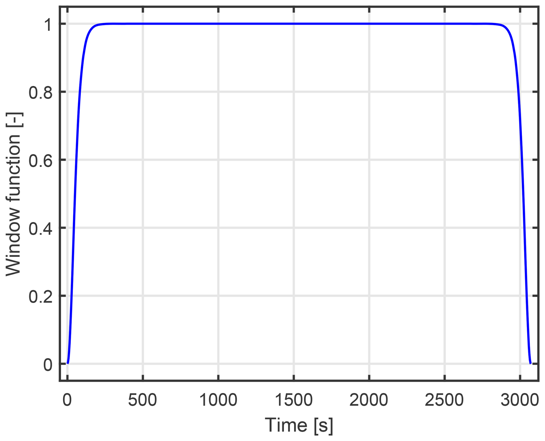
One point worth mentioning is that through the application of the window function, the time span is reduced, where the fast response results can be compared to the benchmark results. As can be seen in Fig. 2, the time lapse valid for comparison between results is located where the window function is equal to 1. The simulation time lost due to windowing (i.e. the portion valid for analysis) is smaller than the time lost due to the initial transient period.

Furthermore, the governing state-space Eq. (17) can be expressed in the frequency domain by converting the time-sampled terms into their frequency-domain representations, yielding

$$\begin{array}{}\text{(22)}& \sum _{s=-N}^N\mathrm{i}{\mathit{\omega }}_{\mathrm{s}}\mathit{q}\left({\mathit{\omega }}_{\mathrm{s}}\right)e^{\mathrm{i}{\mathit{\omega }}_{\mathrm{s}}t}=\sum _{s=-N}^N\left({\left[\mathbf{A}\mathit{q}\right]}_{{\mathit{\omega }}_{\mathrm{s}}}+{\mathit{F}}_B\left({\mathit{\omega }}_{\mathrm{s}}\right)\right)e^{\mathrm{i}{\mathit{\omega }}_{\mathrm{s}}t}.\end{array}$$

The cut-off frequency for the truncation in Eq. (22) must be sufficiently large to cover the wind spectrum. If matrix A is constant, then after simplification of Eq. (22) we get $\left(\mathrm{i}\mathit{\omega }\mathbf{I}-\mathbf{A}\right)\mathit{q}\left(\mathit{\omega }\right)={\mathit{F}}_B\left(\mathit{\omega }\right)$, where I is the identity matrix. Thus, the response vector q(ω) can be computed according to

$$\begin{array}{}\text{(23)}& \mathit{q}\left(\mathit{\omega }\right)=\underset{\mathbf{H}\left(\mathit{\omega }\right)}{\underbrace{{\left(\mathrm{i}\mathit{\omega }\mathbf{I}-\mathbf{A}\right)}^{-\mathrm{1}}}}{\mathit{F}}_B\left(\mathit{\omega }\right),\end{array}$$

which defines the transfer function matrix H(ω). The core principle of fast response calculations is to convert the response solution from the frequency domain to the time domain using the inverse fast Fourier transform (iFFT) algorithm q(t)=ℜ{iFFT{q(ω)}} and then extracting only the real part of the result. The frequency-domain response signal q(ω) must be padded, which involves adding zeros to extend the data to the full length of the original time series before applying the inverse FFT.

To include the contribution of higher harmonics in the response q(t), we take inspiration from Hill's decomposition method for stability analysis of periodic systems and apply a double-sided Fourier decomposition to A_L(t) and q(t). Hill's decomposition is related to previous studies that we performed for response (Pamfil et al., 2024) and stability (Pamfil et al., 2025) analyses.

Hill's decomposition requires first the double-sided Fourier decomposition of time-periodic quantities such as A_L(t) and q(t), which in general can be expressed for any periodic variable X(t) as $\mathbf{X}\left(t\right)={\sum }_{n=-\mathrm{\infty }}^{\mathrm{\infty }}{\mathbf{X}}_n{e}^{\mathrm{i}n\mathrm{\Omega }t}$. In that case, each matrix A_L,n is constant and both variables q(t) and A_L(t) are of dimension N_s. The frequency components X_n of a time-dependent variable X(t) can be obtained using the numerical trapezoidal integration method. For instance, the frequency components A_L,n, associated with A_L(t), can be computed as ${\mathbf{X}}_n=\frac{\mathrm{1}}{T}{\int }_{\mathrm{0}}^T\mathbf{X}\left(t\right)e^{-\mathrm{i}n\mathrm{\Omega }t}\mathrm{d}t$, where $T=\mathrm{2}\mathit{\pi }/\mathrm{\Omega }$ is the period of the system for a given constant rotational speed Ω. Alternatively, since there are sufficient time samples over one period T, the FFT algorithm can be used instead to compute more efficiently the frequency components X_n. The Fourier decomposition is defined as double-sided, ensuring that the system matrix of the LM, A_L(t), the state vector q, and its time derivative $\dot{\mathit{q}}$ remain purely real. This is achieved by the cancellation of the imaginary components arising from the positive (+nΩ) and negative (−nΩ) harmonics, with a truncation upper limit of N=4 in this case study, ensuring an accurate Fourier expansion of A_L(t). As explained in our previous study (Pamfil et al., 2025), the Fourier decomposition of the system matrix A_L(t) from Eq. (19) is valid due to the azimuthal periodicity of the system at a fixed rotational speed Ω. This Fourier decomposition of the state-space variables for the free vibration case was introduced by Hill (1886) and is commonly used for a stability analysis. Hill's theory allows one to carry out a stability analysis of a floating wind turbine while taking into account the rotor's periodicity. For the unforced problem (F_B=0 in Eq. 17), the periodic eigenmodes ψ_k with principle eigenvector components ${\widehat{\mathit{v}}}_{k,n}$, ${\mathit{\psi }}_k={\sum }_{n=-N}^N{\widehat{\mathit{v}}}_{k,n}{e}^{\mathrm{i}n\mathrm{\Omega }t}$ are found by substitution of the solution ${\mathit{\psi }}_{k,\mathrm{sol}}\left(t\right)={\mathit{\psi }}_k{e}^{{\mathit{\lambda }}_{k}t}$, which considers a principal eigenvalue λ_k per mode. This eigenvalue problem leads to the hyper-matrix LTI formulation for the unforced case given by $\widehat{\dot{\mathit{q}}}=\widehat{\mathbf{A}}\widehat{\mathit{q}}$:

$$\begin{array}{}\text{(24)}& \begin{array}{rl}\left[\begin{array}{c}\mathrm{⋮}\\ {\dot{\mathit{q}}}_{n=-\mathrm{1}}\\ {\dot{\mathit{q}}}_{n=\mathrm{0}}\\ {\dot{\mathit{q}}}_{n=\mathrm{1}}\\ \mathrm{⋮}\end{array}\right]& =\left[\begin{array}{ccccc}\mathrm{\ddots }& \mathrm{⋮}& \mathrm{⋮}& \mathrm{⋮}& \mathrm{⋰}\\ \mathrm{\dots }& {\mathbf{A}}_{L,\mathrm{0}}+\mathrm{i}\mathrm{\Omega }\mathbf{I}& {\mathbf{A}}_{L,-\mathrm{1}}& {\mathbf{A}}_{L,-\mathrm{2}}& \mathrm{\dots }\\ \mathrm{\dots }& {\mathbf{A}}_{L,\mathrm{1}}& {\mathbf{A}}_{L,\mathrm{0}}& {\mathbf{A}}_{L,-\mathrm{1}}& \mathrm{\dots }\\ \mathrm{\dots }& {\mathbf{A}}_{L,\mathrm{2}}& {\mathbf{A}}_{L,\mathrm{1}}& {\mathbf{A}}_{L,\mathrm{0}}-\mathrm{i}\mathrm{\Omega }\mathbf{I}& \mathrm{\dots }\\ \mathrm{⋰}& \mathrm{⋮}& \mathrm{⋮}& \mathrm{⋮}& \mathrm{\ddots }\end{array}\right]\\ & \cdot \left[\begin{array}{c}\mathrm{⋮}\\ {\mathit{q}}_{n=-\mathrm{1}}\\ {\mathit{q}}_{n=\mathrm{0}}\\ {\mathit{q}}_{n=\mathrm{1}}\\ \mathrm{⋮}\end{array}\right],\end{array}\end{array}$$

which we have clarified in our work on floating wind turbine stability analysis (Pamfil et al., 2025). $\widehat{\mathbf{A}}$ is referred to as a hyper-matrix because it represents an infinite-dimensional block matrix coupling multiple harmonic components of the state vector. Each entry is itself a matrix acting on the states, resulting in a higher-order structure that can be interpreted as a tensor (or matrix of matrices) indexed by both harmonic components and states. More generally, a hyper-matrix can be viewed as an extension of a conventional matrix to a multi-dimensional array. That being said, we have proven that the formulation of the hyper-matrix $\widehat{\mathbf{A}}$ can be found by replacing the Fourier decomposed terms q(t) and A_L(t) into the state-space Eq. (17) and rearranging them. The corresponding derivations are provided in Eqs. (42), (43), and (44) in our previous paper (Pamfil et al., 2025). Hence, by varying the index n from integer −N to N in Eq. (44) (Pamfil et al., 2025), the row equations of the hyper-matrix expression can be constructed. It should be noted that the harmonic matrices A_L,n required for assembling $\widehat{\mathbf{A}}$ extend from ${\mathbf{A}}_{L,n=-\mathrm{2}N}$ to ${\mathbf{A}}_{L,n=\mathrm{2}N}$. Moreover, under the assumption that the lower harmonics of matrix A_L(t) are greater than the higher harmonics,

$$\begin{array}{}\text{(25)}& \parallel {\mathbf{A}}_{L,\mathrm{0}}{\parallel }_F>\parallel {\mathbf{A}}_{L,\pm \mathrm{1}}{\parallel }_F>\parallel {\mathbf{A}}_{L,\pm \mathrm{2}}{\parallel }_F\mathrm{\dots },\end{array}$$

the constant hyper-matrix $\widehat{\mathbf{A}}$ can be truncated and its eigenvalues would still be accurate.

Although Eq. (24) is derived for the unforced system, it suggests that the original LM may be recast into an LTI system with the hyper-matrix as a constant system matrix. One would need, however, to add the forcing term F_B,L(t), which will generally have frequency content beyond the harmonics of the rotational frequency Ω. Even though the central row in Eq. (24) appears to be the natural position for the forcing term F_B,L(t), this requires a formal assumption. In a previous study that we conducted (Pamfil et al., 2024), for a forced response excitation with a more simplified floating wind turbine model, this approach was tested with a corresponding forcing hyper-vector ${\widehat{\mathit{F}}}_{B,L}\left(t\right)=[\mathrm{\dots },{\mathbf{0}}^T,{\mathit{F}}_{B,L}^T(t),{\mathbf{0}}^T,\mathrm{\dots }{]}^T$ (Pamfil et al., 2024). That produced identical results to the TDM that was linearized, which can be confirmed by inspecting time series in Figs. 6, 7, 16, 17, 18, and 19 (Pamfil et al., 2024). Hence, in Sect. 5, we utilize Eq. (25) to formalize the perturbation methods for fast response computations and de-couple Eq. (24) into smaller subsystems.

To develop novel fast response methods, we take inspiration in Hill's decomposition and assemble a single-sided Fourier series by grouping together the positive and negative harmonic components of the same harmonic order in absolute value. The basis function e^inΩt and the variables q_n and A_L,n are combined with their complex conjugates (denoted as ${\cdot }^{*}$) to form single terms in the single-sided Fourier decomposition. When considering the complex conjugate of a harmonic term X_n, being $X_n^{*}$, it is known that $X_{-n}=X_n^{*}$, which conveys that $\mathrm{\Re }\mathit{\left\{}{X}_{-n}\mathit{\right\}}=\mathrm{\Re }\mathit{\left\{}{X}_n\mathit{\right\}}$ and $\mathrm{\Im }\mathit{\left\{}{X}_{-n}\mathit{\right\}}=-\mathrm{\Im }\mathit{\left\{}{X}_n\mathit{\right\}}$. We apply this notion to obtain single-sided Fourier decompositions of q(t) and A_L(t). Each harmonic component now depends on the real (ℜ{⋅}) and imaginary (ℑ{⋅}) parts for variables q(t) and A_L(t), and for the basis function e^inΩt. This is outlined for the term X(t), which represents either variable q(t) or A_L(t):

$$\begin{array}{}\text{(26)}& \begin{array}{rl}X\left(t\right)& ={\stackrel{\mathrm{̃}}{X}}_{\mathrm{0}}+\stackrel{\mathrm{̃}}{X}\\ & ={\stackrel{\mathrm{̃}}{X}}_{\mathrm{0}}+\sum _{n=\mathrm{1}}^N{\stackrel{\mathrm{̃}}{X}}_n\\ & ={\stackrel{\mathrm{̃}}{X}}_{\mathrm{0}}+\sum _{n=\mathrm{1}}^N\left(X_n{e}^{\mathrm{i}n\mathrm{\Omega }t}+X_{-n}{e}^{-\mathrm{i}n\mathrm{\Omega }t}\right)\\ & ={\stackrel{\mathrm{̃}}{X}}_{\mathrm{0}}+\sum _{n=\mathrm{1}}^N\mathrm{2}\left(\mathrm{\Re }\mathit{\left\{}{X}_n\mathit{\right\}}\mathrm{\Re }\mathit{\left\{}{e}^{\mathrm{i}n\mathrm{\Omega }t}\mathit{\right\}}-\mathrm{\Im }\mathit{\left\{}{X}_n\mathit{\right\}}\mathrm{\Im }\mathit{\left\{}{e}^{\mathrm{i}n\mathrm{\Omega }t}\mathit{\right\}}\right)\\ & ={\stackrel{\mathrm{̃}}{X}}_{\mathrm{0}}+\sum _{n=\mathrm{1}}^N\left(X_{n,c}\cos \left(n\mathrm{\Omega }t\right)+X_{n,s}\sin \left(n\mathrm{\Omega }t\right)\right).\end{array}\end{array}$$

In Eq. (26), the average term X₀ is written as ${\stackrel{\mathrm{̃}}{X}}_{\mathrm{0}}$ instead to ensure consistency in notation. Since the term X(t) is purely real, Eq. (26) demonstrates that the double-sided complex Fourier series (exponential form) can also be expressed as the single-sided real Fourier series (sine-cosine form). The exponential form of the Fourier series translates to a sine-cosine form, where, for each index n, the real cosine and sine coefficients X_n,c and X_n,s are associated with the complex coefficient X_n.

5 Perturbation methods

We develop fast response methods by relying on the Hill expansion for both the LM system matrix A_L and the state response vector q. We recast the Hill expansion instead as a Taylor expansion with a small formal ordering parameter δⁿ which multiplies the corresponding harmonic terms of order n:

$$\begin{array}{}\text{(27)}& \begin{array}{rl}& \mathit{q}\left(t\right)=\sum _{n=-N}^N{\mathit{\delta }}^{\left|n\right|}{\mathit{q}}_n\left(t\right)e^{\mathrm{i}n\mathrm{\Omega }t}={\stackrel{\mathrm{̃}}{\mathit{q}}}_{\mathrm{0}}\left(t\right)+\sum _{n=\mathrm{1}}^N{\mathit{\delta }}^n{\stackrel{\mathrm{̃}}{\mathit{q}}}_n\left(t\right)\\ & {\mathbf{A}}_{\mathrm{L}}\left(t\right)=\sum _{n=-N}^N{\mathit{\delta }}^{\left|n\right|}{\mathbf{A}}_{L,n}{e}^{\mathrm{i}n\mathrm{\Omega }t}={\stackrel{\mathrm{̃}}{\mathbf{A}}}_{L,\mathrm{0}}+\sum _{n=\mathrm{1}}^N{\mathit{\delta }}^n{\stackrel{\mathrm{̃}}{\mathbf{A}}}_{L,n}\left(t\right).\end{array}\end{array}$$

As done in Eq. (26), the negative and positive harmonic terms from the double-sided Fourier expansion $X_{-n}{e}^{-\mathrm{i}n\mathrm{\Omega }t}$ and X_ne^inΩt are combined together as terms of the same harmonic order within a single-sided Fourier series. According to the perturbation method (Bender and Orszag, 1999), the harmonic ordering is explicitly carried out through a perturbative decomposition $X\left(t\right)={\stackrel{\mathrm{̃}}{X}}_{\mathrm{0}}+{\sum }_{n=\mathrm{1}}^N{\mathit{\delta }}^n{\stackrel{\mathrm{̃}}{X}}_n\left(t\right)$, where the harmonic terms originate from the single-sided Fourier series. The higher harmonics response contributions ${\stackrel{\mathrm{̃}}{\mathit{q}}}_n\left(t\right)$ are solved up to a desired order n. In the following Sect. 5.1 and 5.2, we will present the double and single perturbation methods to achieve this.

5.1 Double perturbation method

Our first perturbation method is obtained through insertion of the perturbation expansions from Eq. (27) into the state-space model from Eq. (17). After applying this perturbative decomposition to the state-space ODE terms, we get:

$$\begin{array}{}\text{(28)}& \sum _{n=\mathrm{0}}^N{\dot{\stackrel{\mathrm{̃}}{\mathit{q}}}}_n{\mathit{\delta }}^n=\sum _{p=\mathrm{0}}^N\sum _{j=\mathrm{0}}^N{\stackrel{\mathrm{̃}}{\mathbf{A}}}_{L,j}{\stackrel{\mathrm{̃}}{\mathit{q}}}_p{\mathit{\delta }}^{(p+j)}+{\mathit{F}}_{B,L}.\end{array}$$

The Hill decomposition of the matrix A_L into its harmonics A_L,j can be performed without needing to extract the harmonics from the hyper-matrix $\widehat{\mathbf{A}}$.

Concerning the LM forcing input F_B,L, it is only associated with the unit perturbation of δ⁰=1, which is linked to the zeroth harmonic order. It is generated with the window function W(t) applied (refer to Fig. 2). Continuing from Eq. (28), we can isolate each nth set of equations of the same order of magnitude δⁿ. We can identify the zeroth harmonic equation through the zeroth perturbation order δ⁰, as shown in Eq. (29). The zeroth harmonic response ${\stackrel{\mathrm{̃}}{\mathit{q}}}_{\mathrm{0}}$ can be calculated through the transfer function H(ω) – see Eq. (23).

Bir (2008) has shown that considering only the averaged system matrix ${\stackrel{\mathrm{̃}}{\mathbf{A}}}_{L,\mathrm{0}}$ over a period means neglecting periodic terms that can contribute to the system dynamics. For some load cases, the zeroth-order response ${\stackrel{\mathrm{̃}}{\mathit{q}}}_{\mathrm{0}}$ is insufficient in accounting for the total response q when the latter is highly periodic. This observation has also been noted in the results generated using a more simplified floating wind turbine model – see Fig. 19 of the prior investigation (Pamfil et al., 2024). We have demonstrated (Pamfil et al., 2024) that the zeroth harmonic state response ${\stackrel{\mathrm{̃}}{\mathit{q}}}_{\mathrm{0}}$ is also equivalent to solving in the frequency domain the zeroth-order structural DOF vector ${\stackrel{\mathrm{̃}}{\mathit{x}}}_{\mathrm{0}}\left(\mathit{\omega }\right)$ from the LM EOM (Eq. 14) with zeroth-order mass, damping and stiffness matrices. Furthermore, using the LM EOM is the conventional way of solving the floating wind turbine response in the frequency domain. Consequently, based on Eq. (28), we build a system of equations to solve consecutively higher-order contributions in the following manner:

$$\begin{array}{}\text{(29)}& \begin{array}{ll}{\mathit{\delta }}^{\mathrm{0}}:& {\dot{\stackrel{\mathrm{̃}}{\mathit{q}}}}_{\mathrm{0}}\left(t\right)={\stackrel{\mathrm{̃}}{\mathbf{A}}}_{L,\mathrm{0}}{\stackrel{\mathrm{̃}}{\mathit{q}}}_{\mathrm{0}}+{\mathit{F}}_{B,L}\\ {\mathit{\delta }}^{\mathrm{1}}:& {\dot{\stackrel{\mathrm{̃}}{\mathit{q}}}}_{\mathrm{1}}\left(t\right)={\stackrel{\mathrm{̃}}{\mathbf{A}}}_{L,\mathrm{0}}{\stackrel{\mathrm{̃}}{\mathit{q}}}_{\mathrm{1}}+{\stackrel{\mathrm{̃}}{\mathbf{A}}}_{L,\mathrm{1}}{\stackrel{\mathrm{̃}}{\mathit{q}}}_{\mathrm{0}}\\ & \mathrm{⋮}\\ {\mathit{\delta }}^n:& {\dot{\stackrel{\mathrm{̃}}{\mathit{q}}}}_n\left(t\right)=\sum _{j=\mathrm{0}}^n{\stackrel{\mathrm{̃}}{\mathbf{A}}}_{L,j}{\stackrel{\mathrm{̃}}{\mathit{q}}}_{n-j}={\stackrel{\mathrm{̃}}{\mathbf{A}}}_{L,\mathrm{0}}{\stackrel{\mathrm{̃}}{\mathit{q}}}_n\\ & +\sum _{j=\mathrm{1}}^n{\stackrel{\mathrm{̃}}{\mathbf{A}}}_{L,j}{\stackrel{\mathrm{̃}}{\mathit{q}}}_{n-j},n>\mathrm{0}.\end{array}\end{array}$$

After solving the zeroth harmonic response ${\stackrel{\mathrm{̃}}{\mathit{q}}}_{\mathrm{0}}$, the sequential solving strategy from Eq. (29) is implemented for higher-order harmonic (n>0) responses ${\stackrel{\mathrm{̃}}{\mathit{q}}}_n$. It can be expressed in a lower triangular hyper-matrix form

$$\begin{array}{}\text{(30)}& \left[\begin{array}{c}{\dot{\stackrel{\mathrm{̃}}{\mathit{q}}}}_{\mathrm{0}}\\ {\dot{\stackrel{\mathrm{̃}}{\mathit{q}}}}_{\mathrm{1}}\\ {\dot{\stackrel{\mathrm{̃}}{\mathit{q}}}}_{\mathrm{2}}\\ \mathrm{⋮}\end{array}\right]=\left[\begin{array}{cccc}{\stackrel{\mathrm{̃}}{\mathbf{A}}}_{L,\mathrm{0}}& \mathbf{0}& \mathbf{0}& \mathrm{\dots }\\ {\stackrel{\mathrm{̃}}{\mathbf{A}}}_{L,\mathrm{1}}& {\stackrel{\mathrm{̃}}{\mathbf{A}}}_{L,\mathrm{0}}& \mathbf{0}& \mathrm{\dots }\\ {\stackrel{\mathrm{̃}}{\mathbf{A}}}_{L,\mathrm{2}}& {\stackrel{\mathrm{̃}}{\mathbf{A}}}_{L,\mathrm{1}}& {\stackrel{\mathrm{̃}}{\mathbf{A}}}_{L,\mathrm{0}}& \mathrm{\dots }\\ \mathrm{⋮}& \mathrm{⋮}& \mathrm{⋮}& \mathrm{\ddots }\end{array}\right]\left[\begin{array}{c}{\stackrel{\mathrm{̃}}{\mathit{q}}}_{\mathrm{0}}\\ {\stackrel{\mathrm{̃}}{\mathit{q}}}_{\mathrm{1}}\\ {\stackrel{\mathrm{̃}}{\mathit{q}}}_{\mathrm{2}}\\ \mathrm{⋮}\end{array}\right]+\left[\begin{array}{c}{\mathit{F}}_{B,L}\\ \mathbf{0}\\ \mathbf{0}\\ \mathrm{⋮}\end{array}\right].\end{array}$$

Equation (30) would be solved through a forward substitution similarly to the iterative method of Gauss–Seidel with successive displacement. This iterative solving protocol is identical to the double perturbation method presented in Eq. (29). While the original linear problem expressed through Eqs. (17) and (27) corresponds in Eq. (29) to the sum of the equations in one operation, the perturbation approach breaks this in smaller sub-problems which are solved sequentially.

In summary, the higher-order harmonic responses ${\stackrel{\mathrm{̃}}{\mathit{q}}}_n$ (n>0) are computed successively in the frequency domain (see Eq. 23) as follows:

$$\begin{array}{}\text{(31)}& {\stackrel{\mathrm{̃}}{\mathit{q}}}_n\left(\mathit{\omega }\right)=\underset{\mathbf{H}\left(\mathit{\omega }\right)}{\underbrace{{\left(\mathrm{i}\mathit{\omega }\mathbf{I}-{\stackrel{\mathrm{̃}}{\mathbf{A}}}_{L,\mathrm{0}}\right)}^{-\mathrm{1}}}}\sum _{j=\mathrm{1}}^n{\stackrel{\mathrm{̃}}{\mathbf{A}}}_{L,j}{\stackrel{\mathrm{̃}}{\mathit{q}}}_{n-j}\left(\mathit{\omega }\right),\end{array}$$

where H(ω) is the transfer function and ${\sum }_{j=\mathrm{1}}^n{\stackrel{\mathrm{̃}}{\mathbf{A}}}_{L,j}{\stackrel{\mathrm{̃}}{\mathit{q}}}_{n-j}\left(\mathit{\omega }\right)$ is the numerical forcing term. In the end, we calculate the full response by summing all response harmonics according to Eq. (27) and by converting the solution to the time domain via the iFFT algorithm.

5.2 Single perturbation method

As an alternative to the perturbative expansion in Eq. (27), the system matrix A_L(t) can be expressed as a zeroth- and first-order perturbation of ε, encompassing all higher harmonic contributions, such that ${\mathbf{A}}_{\mathrm{L}}\left(t\right)={\stackrel{\mathrm{̃}}{\mathbf{A}}}_{L,\mathrm{0}}+\mathit{\epsilon }{\stackrel{\mathrm{̃}}{\mathbf{A}}}_{\mathrm{L}}\left(t\right)$. The small perturbation of nth order εⁿ is applied to the response q(t) harmonics and to its time derivative $\dot{\mathit{q}}\left(t\right)$ harmonics. That is equivalent to the double perturbation approach applied to q(t) and $\dot{\mathit{q}}\left(t\right)$, which results in $\mathit{q}\left(t\right)={\stackrel{\mathrm{̃}}{\mathit{q}}}_{\mathrm{0}}+{\sum }_{n=\mathrm{1}}^N{\mathit{\epsilon }}^n{\stackrel{\mathrm{̃}}{\mathit{q}}}_n$. The insertion of these perturbation expressions for A_L(t) and q(t) into Eq. (17) yields

$$\begin{array}{}\text{(32)}& \begin{array}{rl}{\dot{\stackrel{\mathrm{̃}}{\mathit{q}}}}_{\mathrm{0}}& +\sum _{n=\mathrm{1}}^N{\mathit{\epsilon }}^n{\dot{\stackrel{\mathrm{̃}}{\mathit{q}}}}_n={\mathit{F}}_{B,L}+\left({\stackrel{\mathrm{̃}}{\mathbf{A}}}_{L,\mathrm{0}}+\mathit{\epsilon }{\stackrel{\mathrm{̃}}{\mathbf{A}}}_{\mathrm{L}}\right)\\ & \cdot \left({\stackrel{\mathrm{̃}}{\mathit{q}}}_{\mathrm{0}}+\sum _{n=\mathrm{1}}^{N-\mathrm{1}}{\mathit{\epsilon }}^n{\stackrel{\mathrm{̃}}{\mathit{q}}}_n\right)+{\mathit{\epsilon }}^N{\stackrel{\mathrm{̃}}{\mathbf{A}}}_{L,\mathrm{0}}{\stackrel{\mathrm{̃}}{\mathit{q}}}_N.\end{array}\end{array}$$

The cumulative contribution of higher-order harmonics terms is expanded to identify terms for each power of ε. That gives the following sequence of equations that can each be solved through the transfer function H(ω) as in Eq. (31):

$$\begin{array}{}\text{(33)}& \begin{array}{ll}{\mathit{\epsilon }}^{\mathrm{0}}:& {\dot{\stackrel{\mathrm{̃}}{\mathit{q}}}}_{\mathrm{0}}\left(t\right)={\stackrel{\mathrm{̃}}{\mathbf{A}}}_{L,\mathrm{0}}{\stackrel{\mathrm{̃}}{\mathit{q}}}_{\mathrm{0}}+{\mathit{F}}_{B,L}\\ {\mathit{\epsilon }}^{\mathrm{1}}:& {\dot{\stackrel{\mathrm{̃}}{\mathit{q}}}}_{\mathrm{1}}\left(t\right)={\stackrel{\mathrm{̃}}{\mathbf{A}}}_{L,\mathrm{0}}{\stackrel{\mathrm{̃}}{\mathit{q}}}_{\mathrm{1}}+{\stackrel{\mathrm{̃}}{\mathbf{A}}}_{\mathrm{L}}{\stackrel{\mathrm{̃}}{\mathit{q}}}_{\mathrm{0}}\\ & \mathrm{⋮}\\ {\mathit{\epsilon }}^n:& {\dot{\stackrel{\mathrm{̃}}{\mathit{q}}}}_n\left(t\right)={\stackrel{\mathrm{̃}}{\mathbf{A}}}_{L,\mathrm{0}}{\stackrel{\mathrm{̃}}{\mathit{q}}}_n+{\stackrel{\mathrm{̃}}{\mathbf{A}}}_{\mathrm{L}}{\stackrel{\mathrm{̃}}{\mathit{q}}}_{n-\mathrm{1}},n>\mathrm{0}.\end{array}\end{array}$$

In contrast to the double perturbation method, the decomposition of A_L(t) can be achieved without a full Hill expansion, because ${\stackrel{\mathrm{̃}}{\mathbf{A}}}_{L,\mathrm{0}}$ can be calculated by averaging A_L(t) over one period $T=\mathrm{2}\mathit{\pi }/\mathrm{\Omega }$ and ${\stackrel{\mathrm{̃}}{\mathbf{A}}}_L\left(t\right)={\mathbf{A}}_L\left(t\right)-{\stackrel{\mathrm{̃}}{\mathbf{A}}}_{L,\mathrm{0}}$.

Just like for the double perturbation, additional insight can be gained by observing that the single perturbation method in Eq. (33) can be expressed as well by a lower triangular hyper-matrix formulation:

$$\begin{array}{}\text{(34)}& \left[\begin{array}{c}{\dot{\stackrel{\mathrm{̃}}{\mathit{q}}}}_{\mathrm{0}}\\ {\dot{\stackrel{\mathrm{̃}}{\mathit{q}}}}_{\mathrm{1}}\\ {\dot{\stackrel{\mathrm{̃}}{\mathit{q}}}}_{\mathrm{2}}\\ \mathrm{⋮}\end{array}\right]=\left[\begin{array}{cccc}{\stackrel{\mathrm{̃}}{\mathbf{A}}}_{L,\mathrm{0}}& \mathbf{0}& \mathbf{0}& \mathrm{\dots }\\ {\stackrel{\mathrm{̃}}{\mathbf{A}}}_L& {\stackrel{\mathrm{̃}}{\mathbf{A}}}_{L,\mathrm{0}}& \mathbf{0}& \mathrm{\dots }\\ \mathbf{0}& {\stackrel{\mathrm{̃}}{\mathbf{A}}}_L& {\stackrel{\mathrm{̃}}{\mathbf{A}}}_{L,\mathrm{0}}& \mathrm{\dots }\\ \mathrm{⋮}& \mathrm{⋮}& \mathrm{⋮}& \mathrm{\ddots }\end{array}\right]\left[\begin{array}{c}{\stackrel{\mathrm{̃}}{\mathit{q}}}_{\mathrm{0}}\\ {\stackrel{\mathrm{̃}}{\mathit{q}}}_{\mathrm{1}}\\ {\stackrel{\mathrm{̃}}{\mathit{q}}}_{\mathrm{2}}\\ \mathrm{⋮}\end{array}\right]+\left[\begin{array}{c}{\mathit{F}}_{B,L}\\ \mathbf{0}\\ \mathbf{0}\\ \mathrm{⋮}\end{array}\right],\end{array}$$

where the responses ${\stackrel{\mathrm{̃}}{\mathit{q}}}_n$ can be solved similarly to the Gauss–Seidel method of successive displacement (forward substitution).

Finally, the solution of Eq. (33) is computed sequentially in the frequency domain the same way as for the double perturbation method. Once all response harmonics have been computed, they are summed and converted from the frequency domain to the time domain using the inverse fast Fourier transform.

5.3 Laplace transform

An alternative to calculating the system response in the frequency domain using the FFT algorithm is to compute it in the Laplace s domain using the Laplace transform. To calculate the response in the s domain, the system is assumed to be LTI, and the state-space ODE from Eq. (17) is analytically transformed into an algebraic equation. The Laplace method proceeds in the same manner as the Fourier transform, to solve the system response in the new domain and then apply the inverse of the transform to convert it back to the time domain. However, for high-order systems or those with multiple inputs and outputs, performing an analytical symbolic inversion of the Laplace transform can be challenging or impractical, frequently requiring the application of numerical inversion methods. The benefit, in comparison with the Fourier transform method, is that it is capable of considering the initial conditions and transient response, such as for decay tests. The initial condition q(t=0) is taken into account through a time step looping computation procedure where the current time step t_i response is calculated using the previous time step t_i−1, and there is a very small constant time step increment dt. This approach does also simultaneously solve the non-transient response.

Using Eq. (33), we apply the single perturbation approach by carrying out the sum of harmonics response results, i.e. $\stackrel{\mathrm{̃}}{\mathit{q}}={\sum }_{n=\mathrm{0}}^N{\stackrel{\mathrm{̃}}{\mathit{q}}}_n$, only up to the first-order harmonic ${\stackrel{\mathrm{̃}}{\mathit{q}}}_{\mathrm{1}}$. As a starting point, the zeroth harmonic expression that is found in Eq. (33) can be converted to the s domain. This conversion is carried out through the Laplace transform applied on the left- and right-hand side:

$$\begin{array}{}\text{(35)}& \mathcal{L}\left\{{\dot{\stackrel{\mathrm{̃}}{\mathit{q}}}}_{\mathrm{0}}\left(t\right)\right\}={\stackrel{\mathrm{̃}}{\mathbf{A}}}_{L,\mathrm{0}}\mathcal{L}\left\{{\stackrel{\mathrm{̃}}{\mathit{q}}}_{\mathrm{0}}\left(t\right)\right\}+\mathcal{L}\left\{{\mathit{F}}_{B,L}\left(t\right)\right\}t\in [t_{i-\mathrm{1}},t_i].\end{array}$$

The Laplace transform in Eq. (35) is applied locally at each time step t_i over the time interval $[t_{i-\mathrm{1}},t_i]$, which has a duration equal to the time step interval dt. This suggests that the initial condition for that time interval is taken as ${\stackrel{\mathrm{̃}}{\mathit{q}}}_{\mathrm{0}}\left(t_{i-\mathrm{1}}\right)$, and F_B,L(t_i) is assumed to be constant during that time interval.

Although a midpoint evaluation of the forcing vector ${\mathit{F}}_{B,L}(t_{i-\mathrm{1}}+\mathrm{d}t/\mathrm{2})$ is commonly used in staggered time-stepping schemes to achieve a second-order accuracy in time responses q(t), the resulting improvement is not expected to be significant in the present context. Given the chosen sufficiently small time step increment dt, the dominant discrepancies between the linear and time-domain models stem from modelling and linearization assumptions rather than from time integration error. A midpoint forcing would require additional model evaluations at intermediate time instants $t_{i-\mathrm{1}}+\mathrm{d}t/\mathrm{2}$. This would increase the computational cost since the forcing vector time series is already evaluated at each standard discrete time step t_i−1. For these reasons, in the present work, a first-order treatment of the forcing vector is adopted for simplicity and computational efficiency.

In addition, there is no window function W(t) applied here to the forcing term F_B,L(t). After applying the Laplace transform in Eq. (35), it equates to

$$\begin{array}{}\text{(36)}& s{\stackrel{\mathrm{̃}}{\mathit{q}}}_{\mathrm{0}}\left(s\right)-{\stackrel{\mathrm{̃}}{\mathit{q}}}_{\mathrm{0}}\left(t_{i-\mathrm{1}}\right)={\stackrel{\mathrm{̃}}{\mathbf{A}}}_{L,\mathrm{0}}{\stackrel{\mathrm{̃}}{\mathit{q}}}_{\mathrm{0}}\left(s\right)+\underset{{\mathit{F}}_{B,L}\left(s\right)}{\underbrace{{\displaystyle \frac{\mathrm{1}}{s}}{\mathit{F}}_{B,L}\left(t_i\right)}}.\end{array}$$

The s domain contains a real part σ and an imaginary part iω, resulting in $s=\mathit{\sigma }+\mathrm{i}\mathit{\omega }$. The Fourier transform is a particular case of the bilateral Laplace transform where the initial conditions are neglected, i.e. s=iω and σ=0.

Based on Eq. (36), ${\stackrel{\mathrm{̃}}{\mathit{q}}}_{\mathrm{0}}\left(s\right)$ can be isolated:

$$\begin{array}{}\text{(37)}& {\mathcal{L}}^{-\mathrm{1}}\left\{{\stackrel{\mathrm{̃}}{\mathit{q}}}_{\mathrm{0}}\left(s\right)\right\}={\mathcal{L}}^{-\mathrm{1}}\left\{{\left(s\mathbf{I}-{\stackrel{\mathrm{̃}}{\mathbf{A}}}_{L,\mathrm{0}}\right)}^{-\mathrm{1}}\left({\displaystyle \frac{\mathrm{1}}{s}}{\mathit{F}}_{B,L}\left(t_i\right)+{\stackrel{\mathrm{̃}}{\mathit{q}}}_{\mathrm{0}}\left(t_{i-\mathrm{1}}\right)\right)\right\}.\end{array}$$

The inverse of the Laplace transform is applied to solve the state response ${\mathcal{L}}^{-\mathrm{1}}\left\{{\stackrel{\mathrm{̃}}{\mathit{q}}}_{\mathrm{0}}\left(s\right)\right\}={\stackrel{\mathrm{̃}}{\mathit{q}}}_{\mathrm{0}}\left(t_i\right)$, similarly to the inverse of the FFT for the previous fast response methods. The transfer function $\mathbf{H}\left(s\right)={\left(s\mathbf{I}-{\stackrel{\mathrm{̃}}{\mathbf{A}}}_{L,\mathrm{0}}\right)}^{-\mathrm{1}}$ in Eq. (37) is similar to the transfer function for the frequency domain from Eq. (31). The inverse of the Laplace transform is applied to Eq. (37) so that it can be solved only once through a symbolic solver, such as MATLAB's symbolic inverse Laplace function ilaplace. The terms that are a function of the current time step t_i and previous time step t_i−1 are treated as constants when solving symbolically Eq. (37). Also, when solving Eq. (37) numerically at each time step, the time variable t is replaced by the time step increment dt. Afterwards, the same strategy as in Eq. (37) is applied, with a change of variables, to solve the first-order harmonic response ${\stackrel{\mathrm{̃}}{\mathit{q}}}_{\mathrm{1}}\left(t_i\right)$ at time step t_i:

$$\begin{array}{}\text{(38)}& {\mathcal{L}}^{-\mathrm{1}}\left\{{\dot{\stackrel{\mathrm{̃}}{\mathit{q}}}}_{\mathrm{1}}\left(s\right)\right\}={\mathcal{L}}^{-\mathrm{1}}\left\{{\left(s\mathbf{I}-{\stackrel{\mathrm{̃}}{\mathbf{A}}}_{L,\mathrm{0}}\right)}^{-\mathrm{1}}\left({\displaystyle \frac{\mathrm{1}}{s}}{\stackrel{\mathrm{̃}}{\mathbf{A}}}_L{\mathit{q}}_{\mathrm{0}}\left(t_i\right)+{\stackrel{\mathrm{̃}}{\mathit{q}}}_{\mathrm{1}}\left(t_{i-\mathrm{1}}\right)\right)\right\}.\end{array}$$

We impose the initial condition at t=0 for Eq. (38) as ${\stackrel{\mathrm{̃}}{\mathit{q}}}_{\mathrm{1}}\left(t_{\mathrm{1}}\right)=\mathbf{0}$ for the first time step, since ${\stackrel{\mathrm{̃}}{\mathit{q}}}_{\mathrm{0}}\left(t_{\mathrm{1}}\right)=\mathit{q}(t=\mathrm{0})$. Further, as given by Eq. (27), the response ${\stackrel{\mathrm{̃}}{\mathit{q}}}_{\mathrm{1}}\left(t\right)$ is added to the zeroth harmonic solution ${\stackrel{\mathrm{̃}}{\mathit{q}}}_{\mathrm{0}}\left(t\right)$ to obtain the system response q(t).

Due to the computationally expensive time iteration procedure, we settle for an accuracy going up only to the first-order harmonic ${\stackrel{\mathrm{̃}}{\mathit{q}}}_{\mathrm{1}}\left(t\right)$ response. Given the time loop nature of this method, we found out that it was not fast but had a comparable CPU time as the standard time integration of the LM state space. Therefore, for transient response analyses involving longer simulations, it may be more efficient to directly employ the LM approach rather than the single perturbation Laplace transform method. That being said, we benchmark the CPU time and accuracy in the following sections. More details about the computational efficiency are explained in Sect. 7.

6 Results from fast response methods

We present the fast response method time series and the power spectral density (PSD) results for various load cases for the operational point of $V_{\mathrm{0}}=\mathrm{8}\mathrm{m}{\mathrm{s}}^{-\mathrm{1}}$ and $\mathrm{\Omega }=\mathrm{0.6}\mathrm{rad}{\mathrm{s}}^{-\mathrm{1}}$. The simulation duration is T_sim=3071.2 s, as illustrated in Fig. 2, which depicts a window function applied to the time series in the context of a Fourier-based fast response method. Since this study does not include a controller implementation, we select arbitrarily an operational point below the rated wind speed V_r, namely $V_{\mathrm{r}}=\mathrm{11.4}\mathrm{m}{\mathrm{s}}^{-\mathrm{1}}$, as defined for the DTU 10 MW reference wind turbine (Bak et al., 2013). This operational condition is used in this entire paper for all simulation load cases. Results are compared between the TDM, the time-dependent LM, the Fourier-based fast response methods and the Laplace-based method. For the Fourier-based and Laplace-based methods, the zeroth harmonic solution serves as the starting point, and its accuracy is increased through the single and double perturbation (pert.) approaches, with accuracies reaching up to the second harmonic order: O(ε²) and O(δ²), respectively. The TDM results serve as a benchmark to verify if the LM is in accordance with what would be expected but not as a means to evaluate the accuracy of the fast response and Laplace-based results which should rather be compared with the LM. It has been proven in our previous investigations (Pamfil et al., 2024) that the LTI system using Hill's hyper-matrix from Eq. (24), with an accurate Fourier expansion, produces time series results identical to those of the LM. In terms of accuracy analysis for load cases with a stochastic input forcing, the exceedance probabilities for signals are extracted as the positive response peak distance from the mean (steady-state) values.

We compare time- and frequency-domain results for the floater pitch angle ξ₅, as well as the first blade's (l=1) deflection amplitude a₁ and dynamic stall separation function f_s,1. The response results for a single blade only suffice to describe the accuracy of the response calculation methods.

Prior studies using other frequency-domain solvers, such as RAFT, SLOW, and QuLAF, mentioned in the Introduction, do not account for the azimuthal variation of linearized aerodynamic blade loads. Instead, they typically model the rotor load as concentrated at the hub. These studies often compare either frequency- or Laplace-domain results with time-domain simulations obtained from time-domain models, experiments, or higher-fidelity simulations (e.g. computational fluid dynamics or hydro- and aero-elastic solvers). However, they do not investigate different techniques for both frequency- and Laplace-domain simulations of azimuthally dependent linearized aerodynamic loads, nor do they assess the accuracy in comparison to both a linear and a more accurate time-domain model. Furthermore, the simplified floating wind turbine developed in this work offers a lower accuracy compared to more sophisticated aero-elastic solvers. Due to these differences in how aerodynamic and hydrodynamic loads are modelled, direct comparisons with previous models or experimental data are not feasible. The loading and structural modelling approaches used in previous studies differ significantly from the one presented here, limiting the applicability of benchmarking against high-fidelity numerical models or experimental results. Rather than serving as a benchmark tool, the simplified model introduced in this study is intended to explore differences between time-domain, linearized, and fast response methods. Its streamlined formulation provides clear insights into system dynamics and method performance, complementing, rather than replacing, more detailed aero-elastic solvers such as HAWC2, Bladed, OpenFAST, or SIMA.

In this paper, five different load cases are analysed where different inflow velocity and floater pitch moment M_F are considered. The load case distinctions are summarized in Table 1.

Table 1 Simulation load cases for the operational point of $V_{\mathrm{0}}=\mathrm{8}\mathrm{m}{\mathrm{s}}^{-\mathrm{1}}$ and $\mathrm{\Omega }=\mathrm{0.6}\mathrm{rad}{\mathrm{s}}^{-\mathrm{1}}$.

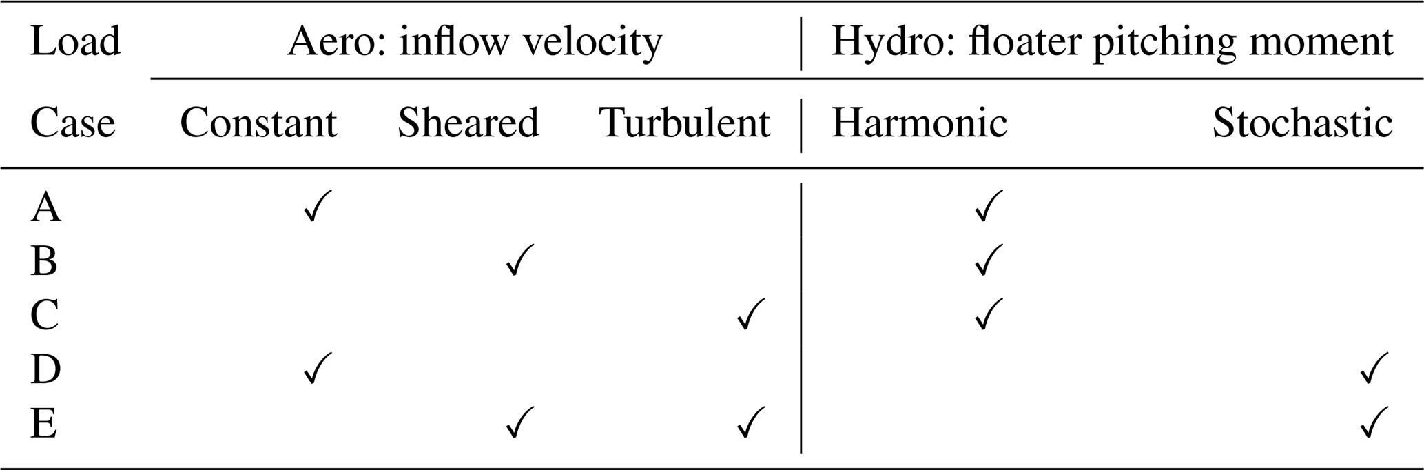
The inflow velocity can be constant, modified by a sheared perturbation, or influenced by coherent turbulence, which is stochastic in nature and characterized by a turbulence intensity (TI) of 5.77 %. Higher TI values, reaching up to 10 % or 15 %, would still satisfy the underlying modelling assumptions. This claim is supported by the results obtained for load cases C and E, which include stochastic wind inflow effects and are presented in Sect. 6.3 and 6.5, respectively. These results indicate that the impact of wind turbulence intensity on the system response can be adequately captured even by a zeroth-order harmonic response, as increasing turbulence intensity leads to a stronger dominance of the zeroth-order harmonic contribution in the system response. As for the floater pitch moment, it can be harmonic or stochastic. Among the load cases presented in Table 1, Case E is considered the most realistic, as it accounts for a stochastic inflow velocity, a stochastic floater pitch moment, and a sheared inflow velocity profile.

6.1 Load Case A: constant inflow and harmonic floater forcing

For the load Case A in Fig. 3, the inflow velocity is constant, and the time series indicate that the zeroth harmonic is insufficient to characterize accurately the blade responses compared to the full LM. A graphically good agreement, however, is seen for the first- and higher-order version of all the fast response methods and the Laplace-based method.

The log-scaled PSD plots in the blade DOFs a₁ and f_s,1 indicate energy peaks at the frequencies distanced at −Ω (−1P) and Ω (1P) away from the floater excitation frequency Ω_M. This demonstrates the frequency coupling caused by the periodic terms in the inertia matrix, also referred to as the mass matrix.

Regarding the floater pitch angle ξ₅, mainly Ω_M is influential on the floater pitch motion considering the high PSD peak occurring at that frequency. The DOF's own natural frequency is not noticeable at ${\mathit{\omega }}_{{\mathit{\xi }}_{\mathrm{5}}}$ because the transient response is omitted in the PSD computation. For the blade DOF PSDs a₁ and f_s,1, the natural frequency ${\mathit{\omega }}_{{\mathit{\xi }}_{\mathrm{5}}}$'s influence on the response is again not visible for the same aforementioned reason.

In a nutshell, the responses show energy peaks caused by the periodic inertia of the system. Due to the presence of a high aerodynamic damping, all results, irrespective of the load case, do not capture the blade's natural frequency ω_1f.

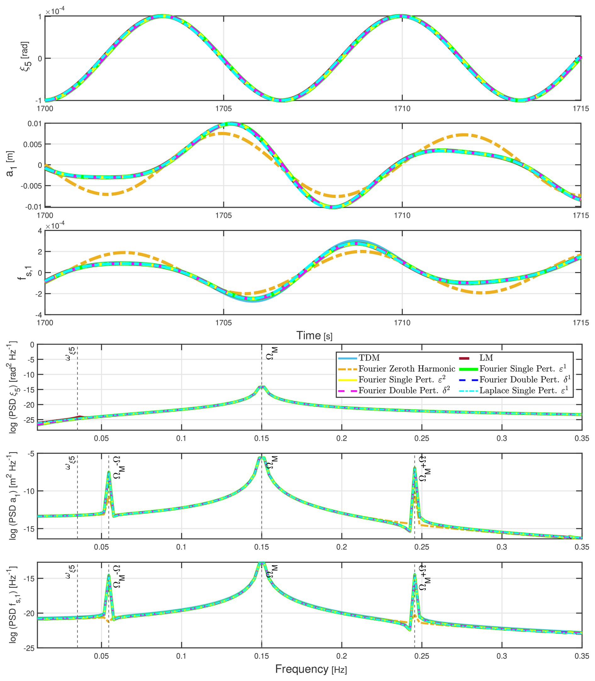
Figure 3 Time series and PSD plots for load Case A with the operational point of $V_{\mathrm{0}}=\mathrm{8}\mathrm{m}{\mathrm{s}}^{-\mathrm{1}}$ and $\mathrm{\Omega }=\mathrm{0.6}\mathrm{rad}{\mathrm{s}}^{-\mathrm{1}}$, and for a simulation duration of T_sim=3071.2 s.

6.2 Load Case B: sheared inflow and harmonic floater forcing

The responses in Fig. 4 for load Case B are associated with a sheared inflow velocity and are highly periodic, as indicated by the PSD plots. The LM, fast response, and Laplace approaches all produce seemingly identical results, where higher-order harmonic corrections do not appear to have any contribution. This implies that the accuracy of the methods is not improved with higher harmonic response considerations for this load case.

The main frequency that is visible in the blade channels a₁ and f_s,1 is Ω (1P) and the floater harmonic excitation frequency Ω_M in the ξ₅ channel. Smaller PSD peaks are observable in the blade channels at the excitation frequencies Ω_M and Ω_M+Ω, with only a barely discernible peak at Ω_M−Ω. The rotational speed frequency Ω is distinguishable in the time series channels for the blade DOFs, due to the strong influence of the sheared inflow, which creates a periodic aerodynamic load. The TDM PSD plots for the blade DOFs a₁ and f_s,1 exhibit additional peaks at integer multiples of the rotational speed, such as 2Ω (2P) and 3Ω (3P). This highlights higher harmonic coupling effects captured by the TDM but not by the LM or by other response methods. Hence, the PSD responses for all methods show dominant peaks at frequencies related to both Ω and Ω_M, including Ω_M+Ω, but only the TDM captures additionally the harmonics 2Ω and 3Ω. This indicates that the TDM system matrix A_T(t) accounts for higher-order coupling mechanisms that emerge at higher harmonic frequencies, most prominently in the f_s,1 channel.

For the floater pitch DOF ξ₅'s channel, like in load Case A, mainly the floater pitch moment excitation frequency Ω_M is captured in the PSD plot, and the sinusoidal motion of the floater is visible in the time series plot. Similarly to the load Case A as well, the natural frequency ${\mathit{\omega }}_{{\mathit{\xi }}_{\mathrm{5}}}$ is not apparent on any channel's PSD plot since the transient response is not taken into account for the PSD calculation.

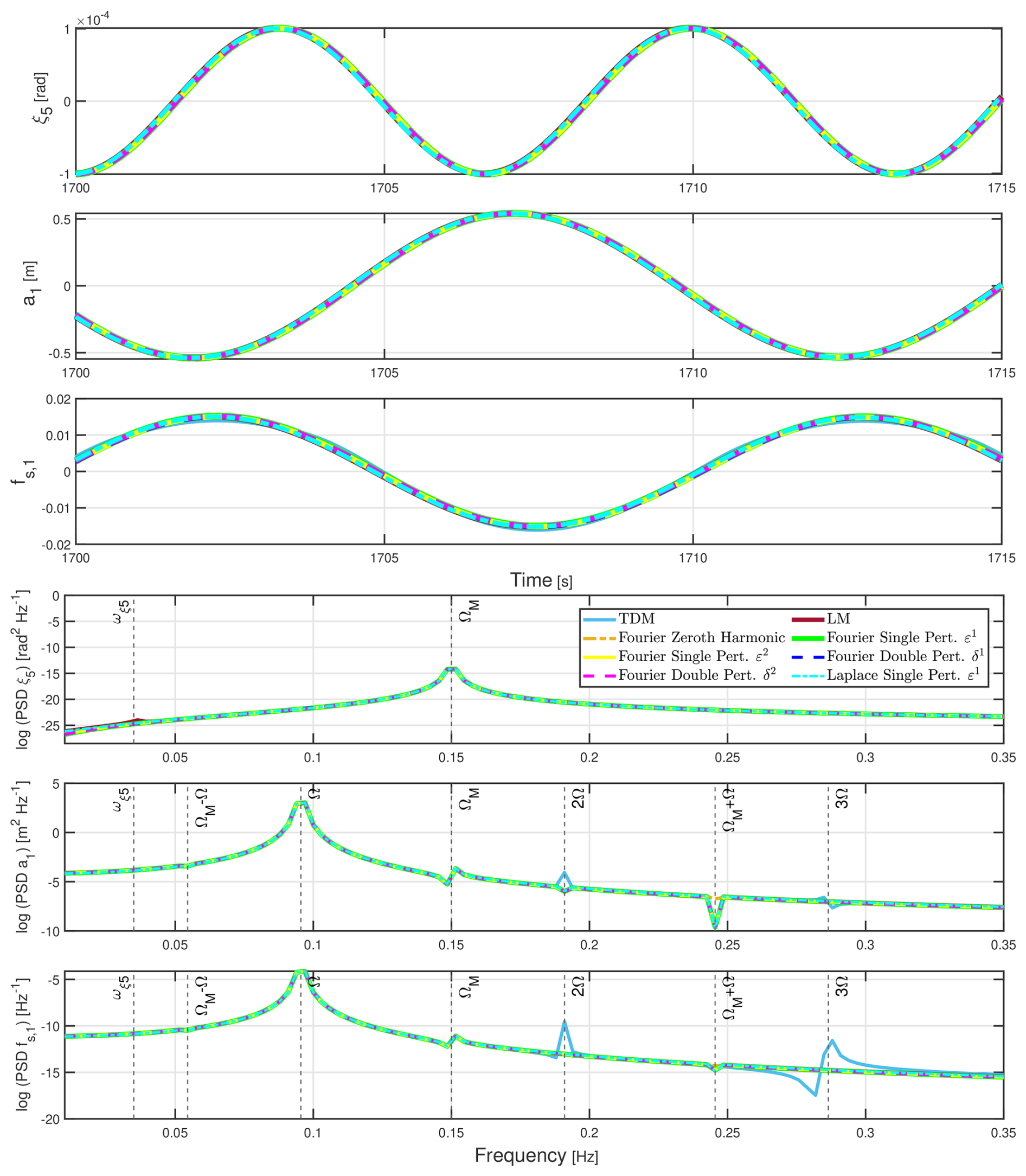
Figure 4 Time series and PSD plots for load Case B with the operational point of $V_{\mathrm{0}}=\mathrm{8}\mathrm{m}{\mathrm{s}}^{-\mathrm{1}}$ and $\mathrm{\Omega }=\mathrm{0.6}\mathrm{rad}{\mathrm{s}}^{-\mathrm{1}}$, and for a simulation duration of T_sim=3071.2 s.

6.3 Load Case C: turbulent inflow and harmonic floater forcing

The load Case C, like all stochastic load cases (C–E), considers a single seed realization (with a TI of 5.77 %) used to present the time series, frequency response, and logarithmic exceedance probability plots. However, for the standard deviation relative error analysis discussed later in Sect. 6.7, various simulations with different TIs were carried out (Fig. C1). As for the simulation duration, it remains the same for all load cases (A–E), with T_sim=3071.2 s.

Concerning the load Case C results displayed in Fig. 5 that are generated for a spatially coherent turbulent inflow velocity, the time series indicate that there is no clear periodic response for the blade variables channels a₁ and f_s,1. Overall, the PSD plots for this stochastic load case illustrate how broad-banded the response spectra are due to the effects of turbulence.

For the f_s,1 channel, the time series show a small offset between the TDM and the other results, while no visible difference is observed between the LM, the Fourier-based fast response methods, and the Laplace-based method.

In the floater pitch angular motion channel, the natural frequency is recognizable at ${\mathit{\omega }}_{{\mathit{\xi }}_{\mathrm{5}}}$ because it is excited by the stochastic load which dominates the response. Further, the energy at the floater pitch excitation frequency Ω_M is visible to a minor degree for the floater pitch motion channel.

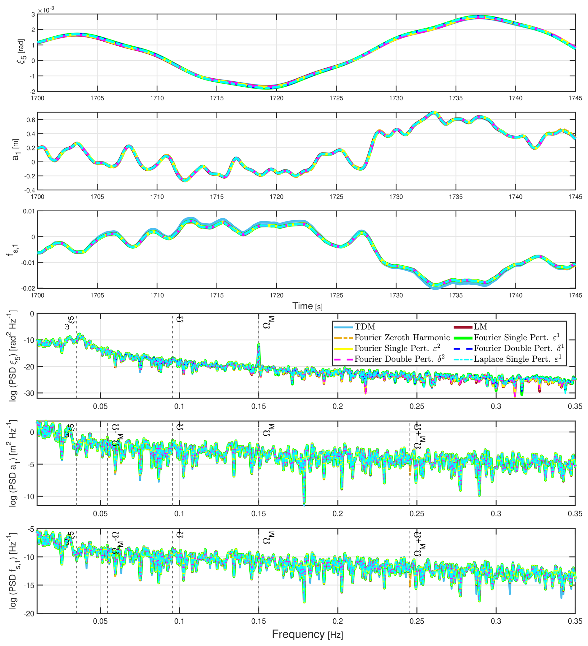
Figure 5 Time series and PSD plots for load Case C with the operational point of $V_{\mathrm{0}}=\mathrm{8}\mathrm{m}{\mathrm{s}}^{-\mathrm{1}}$ and $\mathrm{\Omega }=\mathrm{0.6}\mathrm{rad}{\mathrm{s}}^{-\mathrm{1}}$, and for a simulation duration of T_sim=3071.2 s.

To analyse the accuracy of the various methods in detail, exceedance probability plots are presented in Fig. 6. In this paper, for exceedance probability plots, the absolute value of the relative difference is evaluated at positive peaks corresponding to the same exceedance probability with respect to a reference quantity, typically the LM value. The deviations are generally small between the TDM and LM. The deviation error is obtained by a comparison of two peaks of the same exceedance probability value. The largest ones occur for the f_s,1 channel for the largest peaks with a difference going up to 14 %, whereas it goes up to 5 % for the a₁ channel. The mismatch of higher signal peaks for the fast response and Laplace-based results with the LM occurs at very low exceedance probabilities. This entails that overall results have a good agreement with the LM and that the error is small. The largest deviation from the LM is observed in the a₁ and f_s,1 channels for the fast response single perturbation method of accuracy, going up to O(ε²), resulting in an error reaching 2.8 % for the largest peaks in both channels.

Exceedance probability results are sensitive to small deviations from the LM reference. Consequently, they show that the double perturbation method provides slightly more accurate results than the single perturbation. In addition, for the present load case, an increased harmonic order of consideration (up to perturbation ε² or δ²) does not indicate a considerable improvement in accuracy.

Deviations from the LM also occur for the Laplace method, in particular for the ξ₅ channel result.

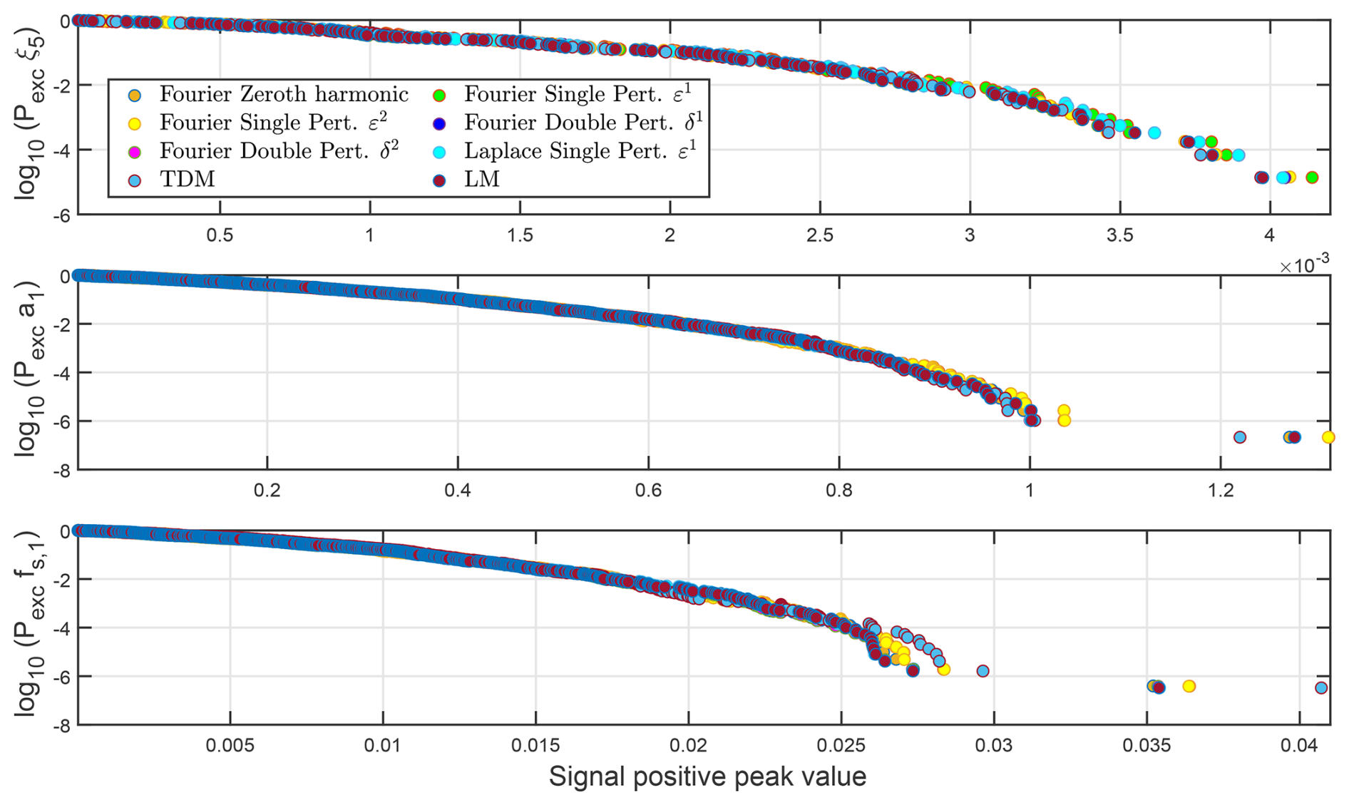
Figure 6 Logarithmic exceedance probability plots for load Case C evaluated for all the fast response methods, the time-domain model (TDM), and the linear model (LM). The operational point is $V_{\mathrm{0}}=\mathrm{8}\mathrm{m}{\mathrm{s}}^{-\mathrm{1}}$ and $\mathrm{\Omega }=\mathrm{0.6}\mathrm{rad}{\mathrm{s}}^{-\mathrm{1}}$, and the simulation duration is of T_sim=3071.2 s.

6.4 Load Case D: constant inflow and stochastic floater forcing

The results for load Case D, shown in Fig. 7, are based on a single seed realization in which the floater pitch moment is stochastic. Also, for the standard deviation relative error analysis of load Case D, presented later in Sect. 6.7, multiple runs with different stochastic seeds for the hydrodynamic moment were performed (Fig. C2).

Generally, the PSD plots for this load case reveal a broad-banded response, as it is influenced by the stochastic nature of the floater pitch moment.

As observed in both the time series and PSD plots, the influence of the periodic system matrix at frequency Ω makes the zeroth harmonic alone insufficient to accurately represent the blade DOF responses compared to methods that include higher harmonic effects. That being said, the comparison between the LM and the fast response and Laplace-based methods shows very good agreement when a higher-order harmonic accuracy is considered. There is also a small offset of the TDM response with the rest of results visible in the f_s,1 channel.

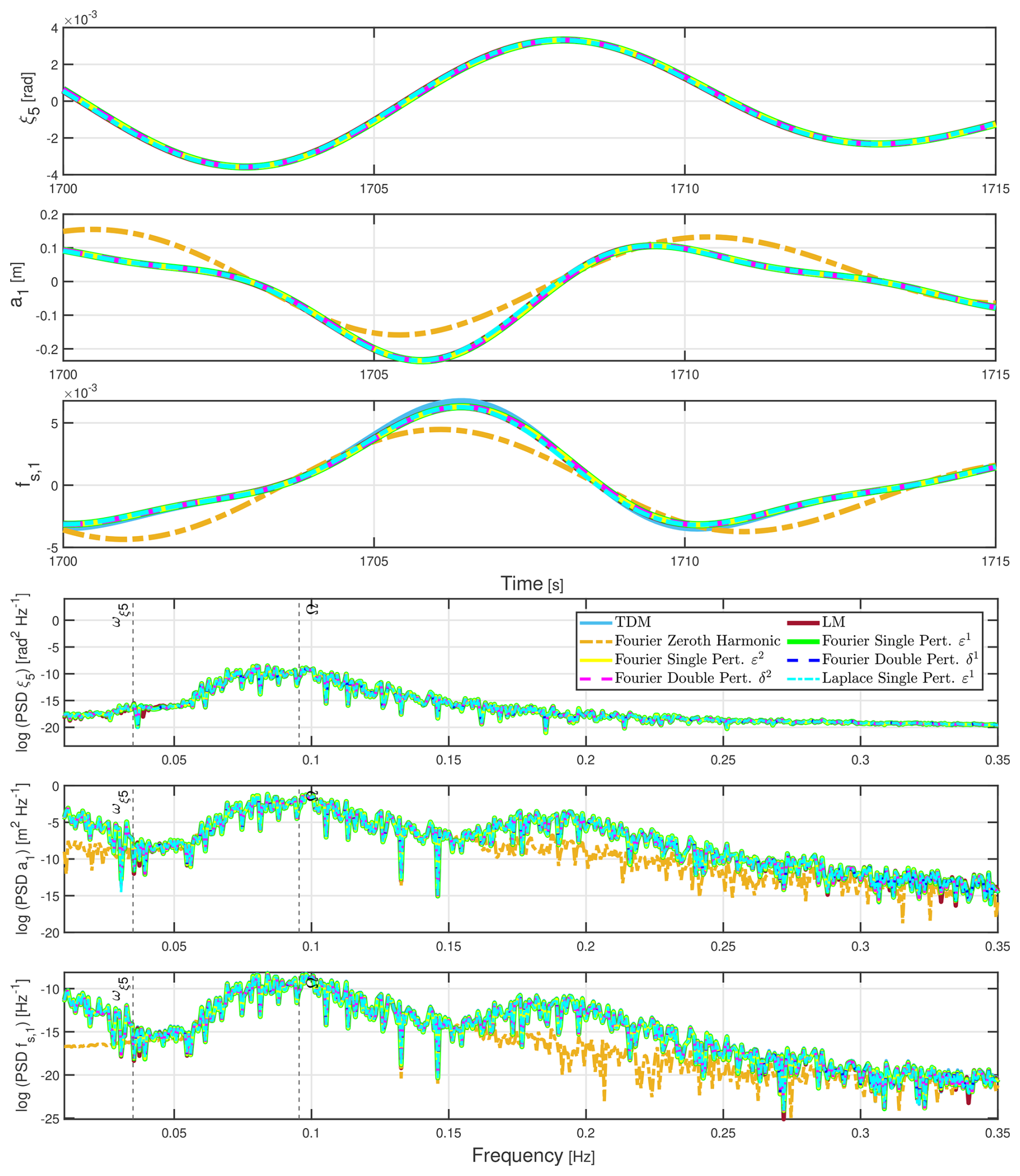
Figure 7 Time series and PSD plots for load Case D with the operational point of $V_{\mathrm{0}}=\mathrm{8}\mathrm{m}{\mathrm{s}}^{-\mathrm{1}}$ and $\mathrm{\Omega }=\mathrm{0.6}\mathrm{rad}{\mathrm{s}}^{-\mathrm{1}}$, and for a simulation duration of T_sim=3071.2 s.

In Fig. 8, consistent with the time series and PSD analyses, the exceedance probability results for load Case D exhibit some discrepancies between the LM and TDM predictions. The largest deviation, reaching an error of 8 %, is observed in the f_s,1 channel. Meanwhile, the zeroth harmonic results accurately approximate the floater pitch response but not the blade responses. Furthermore, the results that include contributions from at least one higher harmonic (fast response methods and the Laplace method) match the LM results perfectly for all channels.

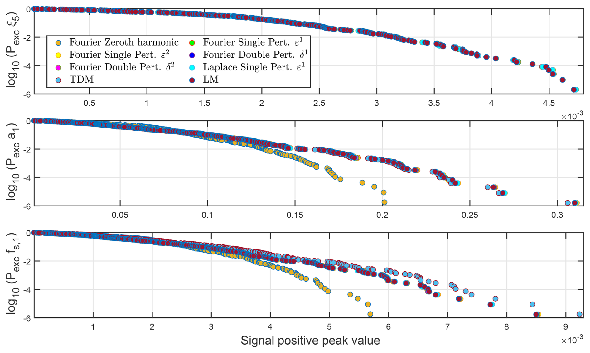
Figure 8 Logarithmic exceedance probability plots for load Case D evaluated for all the fast response methods, the time-domain model (TDM), and the linear model (LM). The operational point is $V_{\mathrm{0}}=\mathrm{8}\mathrm{m}{\mathrm{s}}^{-\mathrm{1}}$ and $\mathrm{\Omega }=\mathrm{0.6}\mathrm{rad}{\mathrm{s}}^{-\mathrm{1}}$, and the simulation duration is of T_sim=3071.2 s.

6.5 Load Case E: shear, turbulent inflow, and stochastic floater forcing

Finally, for the load Case E, where both the inflow velocity and the floater pitch moment are stochastic, the results are showcased in Fig. 9. PSD plots for the stochastic load Case E reveal how broad frequency the response is due to the influence of turbulent inflow. The peak for the rotational speed frequency Ω is noticeable in the floater pitch ξ₅ PSD channel, but it is most apparent in the blade DOF channels. Yet, it was also present on PSD plots for Case D, but that peak was highly damped in comparison. Generally, the results for the Laplace and fast response methods that are above the zeroth harmonic in accuracy match well with the LM.

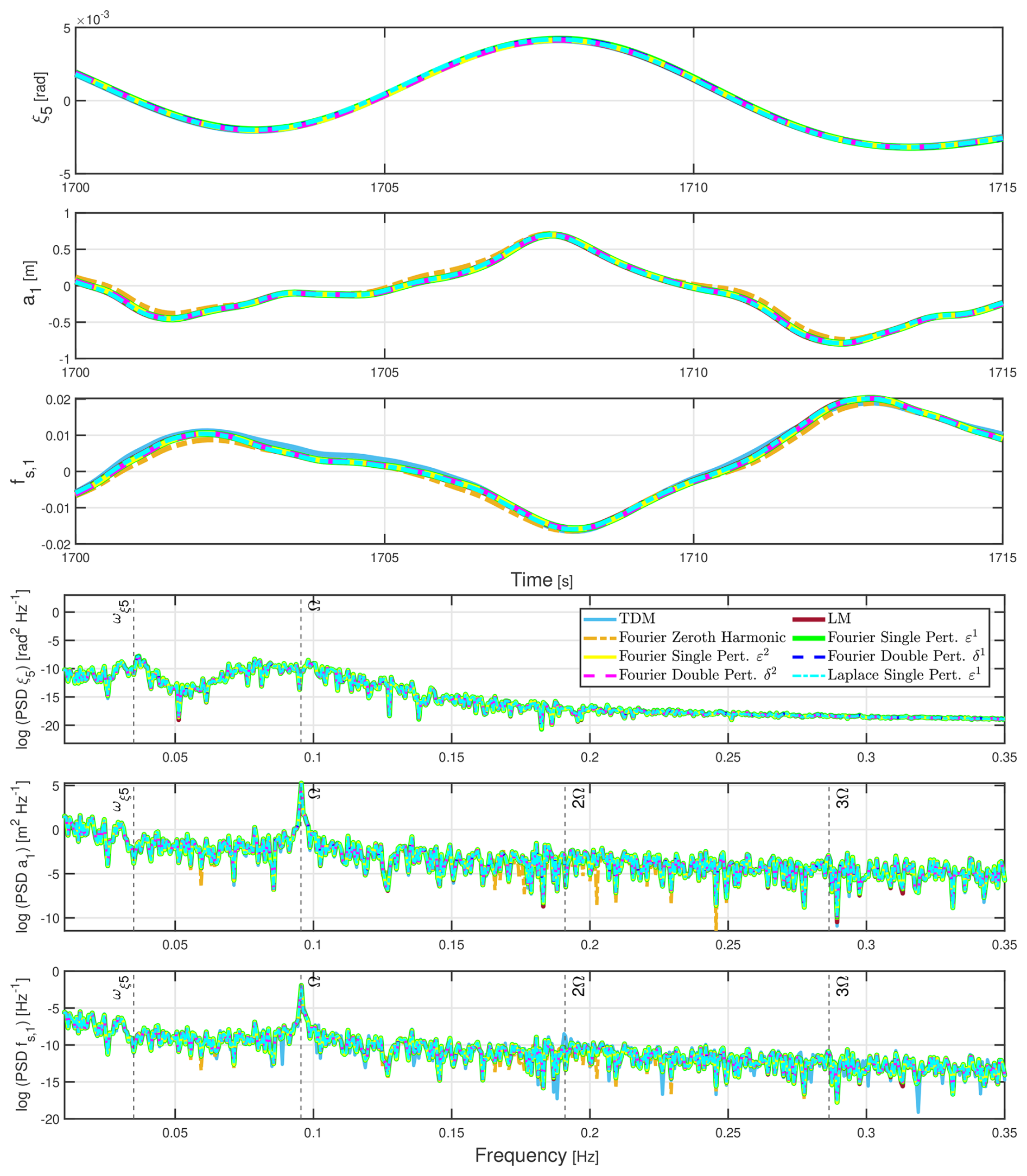
Figure 9 Time series and PSD plots for load Case E with the operational point of $V_{\mathrm{0}}=\mathrm{8}\mathrm{m}{\mathrm{s}}^{-\mathrm{1}}$ and $\mathrm{\Omega }=\mathrm{0.6}\mathrm{rad}{\mathrm{s}}^{-\mathrm{1}}$, and for a simulation duration of T_sim=3071.2 s.

The load Case E exceedance probability results are shown in Fig. 10. They overlap each other for the most part, except for the TDM results in the blade DOF channels a₁ and f_s,1. Just like for the time series, the exceedance probability results for the methods having an accuracy that is above the zeroth harmonic methods agree well with the LM results. In that respect, the largest errors occurring in the a₁ and f_s,1 channels under load Case E reach a maximum of approximately 1.3 %. There are additional deviations of the Laplace method from the LM results that appear in the ξ₅ channel and which are of 1.6 % error in magnitude.

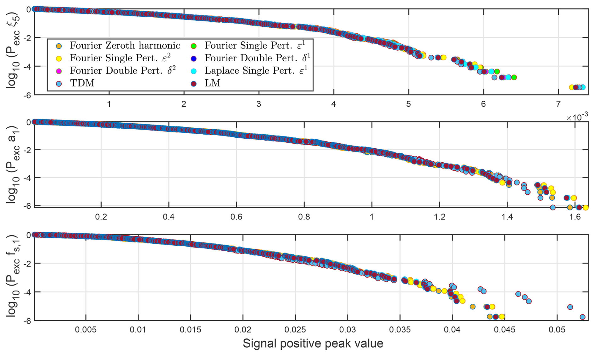
Figure 10 Logarithmic exceedance probability plots for load Case E evaluated for all the fast response methods, the time-domain model (TDM), and the linear model (LM). The operational point is $V_{\mathrm{0}}=\mathrm{8}\mathrm{m}{\mathrm{s}}^{-\mathrm{1}}$ and $\mathrm{\Omega }=\mathrm{0.6}\mathrm{rad}{\mathrm{s}}^{-\mathrm{1}}$, and the simulation duration is of T_sim=3071.2 s.

6.6 Overview

Overall, a noticeable discrepancy in results occurs between the TDM and LM. That is to be expected due to the non-linear effects that the TDM takes into account with the time variability of aerodynamic variables. However, for most load cases, the results of the perturbation methods matched well with the LM reference. The deviations from the LM are not always perceptible in time series excerpts and PSD plots. They become noticeable in exceedance probability plots with an increasing signal peak value and a reduced probability.

An important mismatch is observed between the zeroth harmonic response and responses of a higher harmonic-order consideration. The inaccuracy of the zeroth harmonic response is visible in time series and PSD plots, and particularly in exceedance probability plots where deviations from the LM reference are most apparent. This occurs when the forcing contains a high periodicity with Ω for a specific load case. The high periodicity of the load refers to its frequency spectrum being highly influenced by the integer harmonics of the rotational speed Ω, resulting in pronounced spectral peaks at those harmonic frequencies.

The zero-order method shows large deviations, especially in load cases A and D (i.e. cases with constant wind). As discussed earlier, turbulent wind, particularly at higher TI, enhances the dominance of the zeroth-order response through its contribution to the state-space forcing vector F_B,L(t). In contrast, under constant wind inflow, the zeroth-order response is less dominant because F_B,L(t) is not influenced by variations in the inflow velocity ΔV_0,l for blade index l. For these load cases, the resulting large relative errors are reflected in both the blade response and the dynamic stall degrees of freedom, as their excitation relies primarily on floater pitch motion due to the constant wind. This leaves the dynamic forcing of these blade DOFs to be caused through the floater pitch motion. In the present floating wind turbine model, this coupling involves the mass matrix, which is assumed constant at zeroth order, thereby limiting the representation of periodic effects.

To provide an overview of the accuracy of the results, the exceedance probability error is compared in terms of the signal positive peak value relative to the LM at the level of $P_{\text{exc}}={\mathrm{10}}^{-\mathrm{2}}$ and at the highest peak level, labelled $P_{\text{exc}}={\mathrm{10}}^{-x}$. If the relative error with respect to the LM is higher at another exceedance probability level than at the highest peak, which can sometimes occur (e.g. load Case E), then the error is evaluated at that level. Besides, the relative error can be evaluated for the stochastic load cases C, D, and E, across the different response channels ξ₅, a₁, and f_s,1, and various response (Resp.) calculation methods. The response calculation methods include the Fourier single perturbation method with accuracy ε² (S2), the double perturbation method with accuracy δ² (D2), and the Laplace single perturbation method with accuracy ε¹ (L1). The relative error results for these three methods are presented in Table 2.

Table 2 Exceedance probability relative error in percentage ( %) for signal positive peak value with respect to LM reference for the operational point of $V_{\mathrm{0}}=\mathrm{8}\mathrm{m}{\mathrm{s}}^{-\mathrm{1}}$, $\mathrm{\Omega }=\mathrm{0.6}\mathrm{rad}{\mathrm{s}}^{-\mathrm{1}}$.

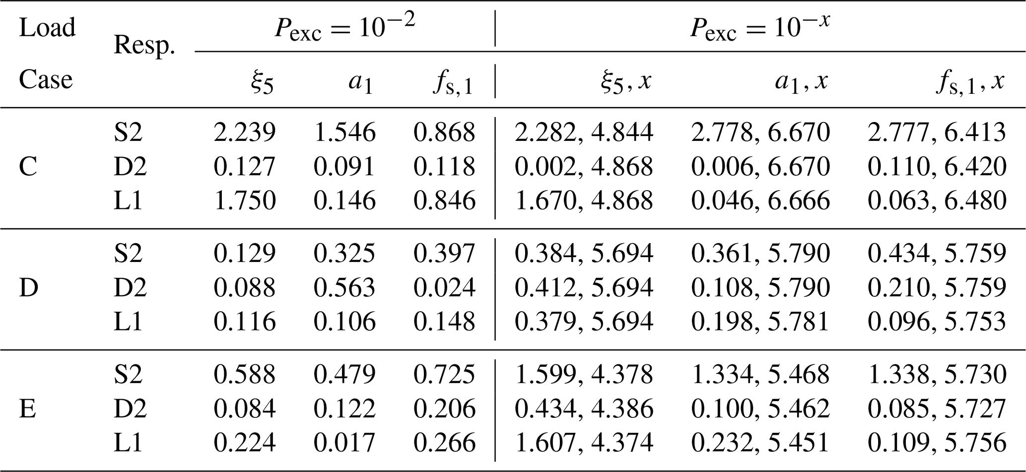
To reduce the size of Table 2, only the higher-order results are presented here, as these correspond to the highest accuracy for each perturbation-based method. Even though the zeroth-order results appear to perform well for the stochastic load cases C (Figs. 5 and 6) and E (Figs. 9 and 10), they are not shown here. According to the relative error results in Table 2, the D2 method generally provides the highest response precision, while the L1 method occasionally outperforms it depending on the load case and the exceedance probability level considered. The overall accuracy of these two methods is excellent, with the highest observed relative error not exceeding 0.56 %. In contrast, the S2 method consistently yields the lowest accuracy across most load cases and exceedance probability levels, with relative errors systematically higher than those of the D2 and L1 methods. This discrepancy is particularly notable in the estimation of the ξ₅ channel response, where the S2 method often underperforms compared to its counterparts. The largest error for the S2 method is 2.78 %, which is still fairly accurate.

6.7 Standard deviation relative error

The accuracy of the fast response methods can be alternatively quantified through the standard deviation relative error (SDRE), which is denoted ${\mathit{\sigma }}_{\mathrm{SDRE}}\left({\stackrel{\mathrm{̃}}{q}}_{i,\mathrm{method}}\left(t\right)\right)$ and evaluated for each ith response channel's non-transient data samples. It is calculated through the standard deviation (σ(⋅)) of the data samples' residual with respect to the LM reference values ${\stackrel{\mathrm{̃}}{q}}_{i,\mathrm{LM}}\left(t\right)$ and then normalized with respect to the standard deviation of the LM values:

$$\begin{array}{}\text{(39)}& {\mathit{\sigma }}_{\mathrm{SDRE}}\left({\stackrel{\mathrm{̃}}{q}}_{i,\mathrm{method}}\left(t\right)\right)={\displaystyle \frac{\mathit{\sigma }\left({\stackrel{\mathrm{̃}}{q}}_{i,\mathrm{method}}\left(t\right)-{\stackrel{\mathrm{̃}}{q}}_{i,\mathrm{LM}}\left(t\right)\right)}{\mathit{\sigma }\left({\stackrel{\mathrm{̃}}{q}}_{i,\mathrm{LM}}\left(t\right)\right)}}.\end{array}$$

Evidently, a higher SDRE value translates to a lower accuracy. Compared to the analysis of exceedance probability plots in Figs. 6, 8 and 10, this error measure concerns a direct deterministic comparison of the response time series. The SDRE accuracy values are visualized for the fast response and Laplace methods in comparison to the LM benchmark in Fig. 11.

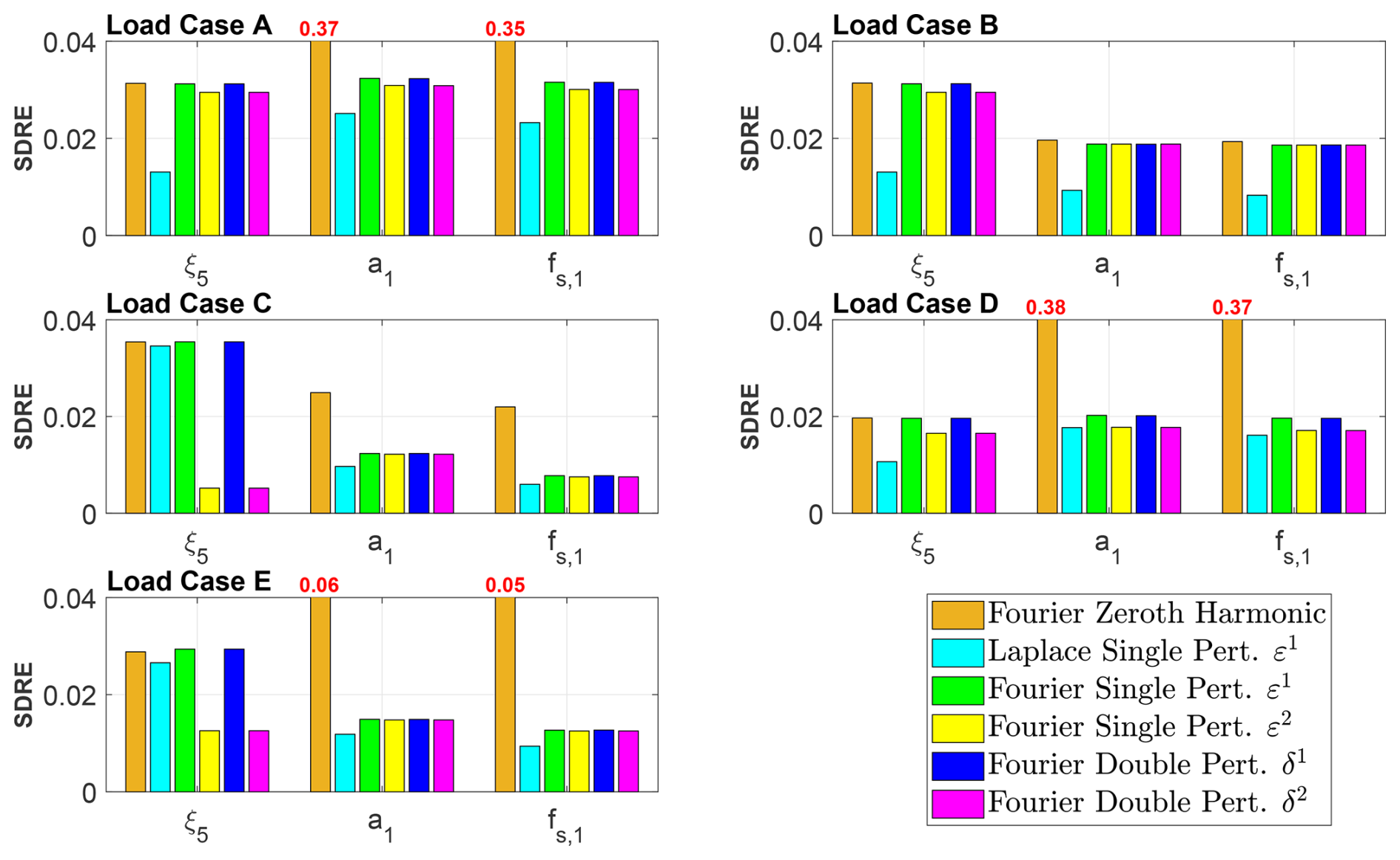
Figure 11 Standard deviation relative error (SDRE) for varying load cases and response channels. The analysed fast response methods are the Fourier zeroth harmonic, as well as the double and single perturbation (pert.) methods.

Results in Fig. 11 confirm roughly the same observations as deduced from exceedance probability plots and time series. For the single and double perturbation methods, the accuracy was first tested for a precision up to first-order harmonic (ε¹ and δ¹ perturbation). Then the response accuracy was increased up to second-order harmonic (ε² and δ² perturbation), which did improve it considerably for the ξ₅ channel in load cases C and E, whereas it did not affect it significantly for other load cases. This supports the choice of settling for a maximal second-order harmonic accuracy being tested for both the single and double perturbation methods.

The zeroth harmonic method can result in error levels of up to 38 % for certain load cases, as demonstrated by the corresponding time series, PSD, and logarithmic exceedance probability plots. Meanwhile, the error levels of both first-order methods, including single and double perturbation, remain below 3.5 % across all tests. For load Case E, the difference in SDRE values between the zeroth-order and higher-order methods is somewhat larger than expected, based on the time series, PSD, and logarithmic exceedance probability plots (Figs. 9 and 10). This occurs even though the SDRE values for the zeroth-order channels remain below 6 %. The discrepancy can be attributed to the slight deviations of the zeroth-order responses from the other responses in the blade channels a₁ and f_s,1, as observed in the time series and PSD plots shown in Fig. 9. In addition, for some of the tests, the second-order methods improve the accuracy relative to the first-order methods. Thus, for example, in the stochastic load cases C, D, and E, they give error levels of below 2 %. As for the Laplace single perturbation method of ε¹ perturbation order, its accuracy fluctuates more than for fast responses but is below 3.5 % for all load cases.

Moreover, there are some important numerical attributes of the system matrices worth noting that explain why part of the results are not always affected by the load case itself in this study.

First, the time-varying components of the system matrix ${\stackrel{\mathrm{̃}}{\mathbf{A}}}_{\mathrm{L}}$ can be approximated by only the first-order harmonic contribution ${\stackrel{\mathrm{̃}}{\mathbf{A}}}_{L,\mathrm{1}}$, meaning that other higher-order harmonics, including ${\stackrel{\mathrm{̃}}{\mathbf{A}}}_{L,\mathrm{2}}$, are negligible, i.e. ${\stackrel{\mathrm{̃}}{\mathbf{A}}}_{\mathrm{L}}\approx {\stackrel{\mathrm{̃}}{\mathbf{A}}}_{L,\mathrm{1}}$ and ${\stackrel{\mathrm{̃}}{\mathbf{A}}}_{L,\mathrm{2}}\approx \mathbf{0}$. Under this observation, the single and double perturbation numerical schemes produce identical accuracy results in terms of SDRE value. This implication is discernible through a comparison of the single and double perturbation Eqs. (34) and (30), respectively. These equations are equal if we neglect the term ${\stackrel{\mathrm{̃}}{\mathbf{A}}}_{L,\mathrm{2}}{\stackrel{\mathrm{̃}}{\mathit{q}}}_{\mathrm{0}}\approx \mathbf{0}$ in Eq. (30). That explains why for most load cases the error levels do not decrease significantly from first- to second-order harmonic response and that the single and double perturbation methods show broadly an identical accuracy.

Second, the off-diagonal terms in Eqs. (34) and (30) are forcing input contributions that multiply the transfer function H(ω). When solving the first-order harmonic ${\stackrel{\mathrm{̃}}{\mathit{q}}}_{\mathrm{1}}$, the forcing contribution is only determined by ${\stackrel{\mathrm{̃}}{\mathbf{A}}}_L{\stackrel{\mathrm{̃}}{\mathit{q}}}_{\mathrm{0}}$ or ${\stackrel{\mathrm{̃}}{\mathbf{A}}}_{L,\mathrm{1}}{\stackrel{\mathrm{̃}}{\mathit{q}}}_{\mathrm{0}}$ depending on the method (single or double perturbation). For the ξ₅ channel in all load cases, this numerical forcing term happens to produce almost a null first-harmonic response ${\stackrel{\mathrm{̃}}{\mathit{q}}}_{\mathrm{1}}\approx \mathbf{0}$. In this scenario, the zeroth harmonic response ${\stackrel{\mathrm{̃}}{\mathit{q}}}_{\mathrm{0}}$ magnitude (Euclidean norm) is much greater than the corresponding DOF coefficients in ${\stackrel{\mathrm{̃}}{\mathbf{A}}}_{L,\mathrm{1}}$ (Frobenius norm). This indicates that the coupling between these two terms of varying harmonic is indeed negligible, which is why there is no added accuracy in SDRE when adding the first-order harmonic contribution to the zeroth order for the ξ₅ channel.

One of the major distinctions between load case accuracy is observable for the floater pitch channel ξ₅ when the load case considers the stochastic forcing from a turbulent inflow or a stochastic hydrodynamic moment. According to the corresponding PSDs for load cases C, D, and E in Figs. 5, 7, and 9, there is a peak at the rotational speed Ω (1P). The peak at 1P frequency occurs within the power spectra in the ξ₅ channel for load Case C, and in the blade DOF channels a₁ and f_s,1 for load cases D and E in particular. For these particular scenarios, the Ω frequency of excitation signifies that the system is influenced by the corresponding first-order harmonic response ${\stackrel{\mathrm{̃}}{\mathit{q}}}_{\mathrm{1}}$. Given that ${\stackrel{\mathrm{̃}}{\mathit{q}}}_{\mathrm{1}}$ is non-negligible for load cases C, D, and E, the evaluation of the forcing term ${\stackrel{\mathrm{̃}}{\mathbf{A}}}_{L,\mathrm{1}}{\stackrel{\mathrm{̃}}{\mathit{q}}}_{\mathrm{1}}$ for the double perturbation method and ${\stackrel{\mathrm{̃}}{\mathbf{A}}}_L{\stackrel{\mathrm{̃}}{\mathit{q}}}_{\mathrm{1}}$ for the single perturbation method improves the model accuracy through the contribution of a second-order harmonic ${\stackrel{\mathrm{̃}}{\mathit{q}}}_{\mathrm{2}}$ in the response q. This improvement in accuracy translates to a decrease in SDRE for the ξ₅ channels.

The SDRE has also been evaluated individually for load Case C, considering variations in the stochastic inflow TI, and for load Case D, by repeating simulation runs with different seeds for the stochastic hydrodynamic moment. The findings for the variation of TI in load Case C and the different runs in load Case D are illustrated in Appendices C1 and C2, respectively. According to the corresponding two Figs. C1 and C2, there is a visibly stronger variation of SDRE values for the load Case C, with changes in the inflow TI, compared to the load Case D, with different simulation runs and different inputs of stochastic hydrodynamic moments. For load Case D, changes in the stochastic seed have minimal impact on the bar plots, while TI variations for load Case C have a slightly more pronounced effect on the SDRE results.

Starting from the analysis of the SDRE for all load Cases A to E in Fig. 11, it is clear that the variability in the SDRE values is not due to random noise but reflects a method-dependent sensitivity to different stochastic excitations. To rigorously assess these differences for all response methods, non-parametric statistical tests were applied. They are more suitable than traditional parametric approaches, such as the analysis of variance (ANOVA) or t-tests which presume normality and equal variances of responses. Non-parametric tests were performed due to the non-Gaussian and non-linear nature of the system responses under turbulent and stochastic hydrodynamic moment inputs. In particular, the Kruskal–Wallis test was used for independent sample comparisons in order to treat responses from each method as unrelated, while the Friedman test accounted for repeated response measures when the same system was analysed using different estimation methods. The Kruskal–Wallis statistical analysis produced p values (probability values) well below the 0.05 threshold for load cases C (turbulent inflow) and D (stochastic hydrodynamic loading), and for all three output channels ξ₅, a₁, and f_s,1. This indicates statistically significant differences between the estimation methods. When all load cases (A–E) were considered, the p values increased slightly above 0.05, suggesting that the influence of the method becomes more diffuse across a broader range of conditions. This observation is logical, as the influence of the method on the SDRE value is more pronounced across varying load cases A to E than across the variation of TI in load Case C. In that vein, the lowest p values are observed for load Case D, as the variation between simulation runs has less impact on the SDRE compared to the more substantial changes introduced in the other load case groupings. The Friedman test results revealed that across all load conditions, including the combined set A to E, p values remained consistently below 0.01 for all three response channels. This suggested a stronger and more systematic impact of the estimation method when repeated measures from the same simulations were considered.

While both the Kruskal–Wallis and Friedman tests indicated that at least one method differs from the others, they did not reveal which ones. Therefore, post-hoc pairwise comparisons were conducted to identify the specific method pairs with statistically significant differences. Hence, the post-hoc tests revealed for each channel and load case scenario which pairs of methods differ the most from each other and which method stands out from other methods. In general, the zeroth harmonic and Laplace methods consistently showed statistically significant differences compared to other methods across most load case scenarios and response channels. This is to be expected, since the single and double perturbation methods follow a similar computational approach.

7 Fast response method efficiency analysis

We now evaluate the execution time for various durations of the simulated time series. Such comparison involves several choices that can significantly affect the results, including the simulation time step interval dt, the load case being simulated, and the structure of the code. For instance, the simulation time step increment was set to dt=0.0937 s, which corresponds to a Nyquist frequency of 5 Hz. The computational efficiency study was only carried out for load Case E, because it is more realistic due to its stochastic nature both in wind inflow and hydrodynamic moment. It is worth noting that this section addresses the computational cost of time-domain simulations using either the TDM or LM, as well as alternative formulations in the frequency domain (Fourier based) and the Laplace domain (s domain). The developed fast response methods are aimed at time-domain simulations, where rainflow-count-based fatigue analysis and exceedance probability analysis are possible. The use of the frequency domain is adopted solely to enhance numerical efficiency.

Efficient implementations were assembled for both the single and double perturbation methods by avoiding looping over time steps when possible. Looping over time steps is, however, unavoidable for the Laplace single perturbation method approach and when generating the system forcing time series F_B,L(t). But the inverted structural mass matrix ${\mathbf{M}}_{\mathrm{S}}^{-\mathrm{1}}\left(t\right)$ that affects F_B,L(t) can be pre-computed for all time steps.

Since the new response methods require some pre-processing, CPU time can be saved by storing these results. This is outlined for the different response calculation methods in Appendix D, distinguishing between the first simulation for one random seed (Seed 1) and the subsequent simulation of a new seed (Seed 2). The hardware configuration used for computations was an HP EliteBook 840 G8 Notebook PC that features an Intel Core i7-1185G7 processor with four cores, eight threads, and a base clock of 2.99 GHz, with up to 4.8 GHz turbo boost. Regarding the programming implementation in MATLAB of the response calculations, there was no parallelization strategy. Not using parallelization in fast response analysis programming can be advantageous because it minimizes overhead costs, decreases latency, and enhances predictability. This simpler approach also improves cache efficiency and eliminates the complexities and synchronization delays that are often encountered in parallel processing. If more cores are available, several load cases can be run independently in parallel. The CPU time of the TDM and LM for load Case E is shown in Fig. 12 with a log-log scale on the x and y axes. Figure 12 also presents CPU time results for a Seed 1 for the fast response methods and a Seed 2, as well for the Laplace method.

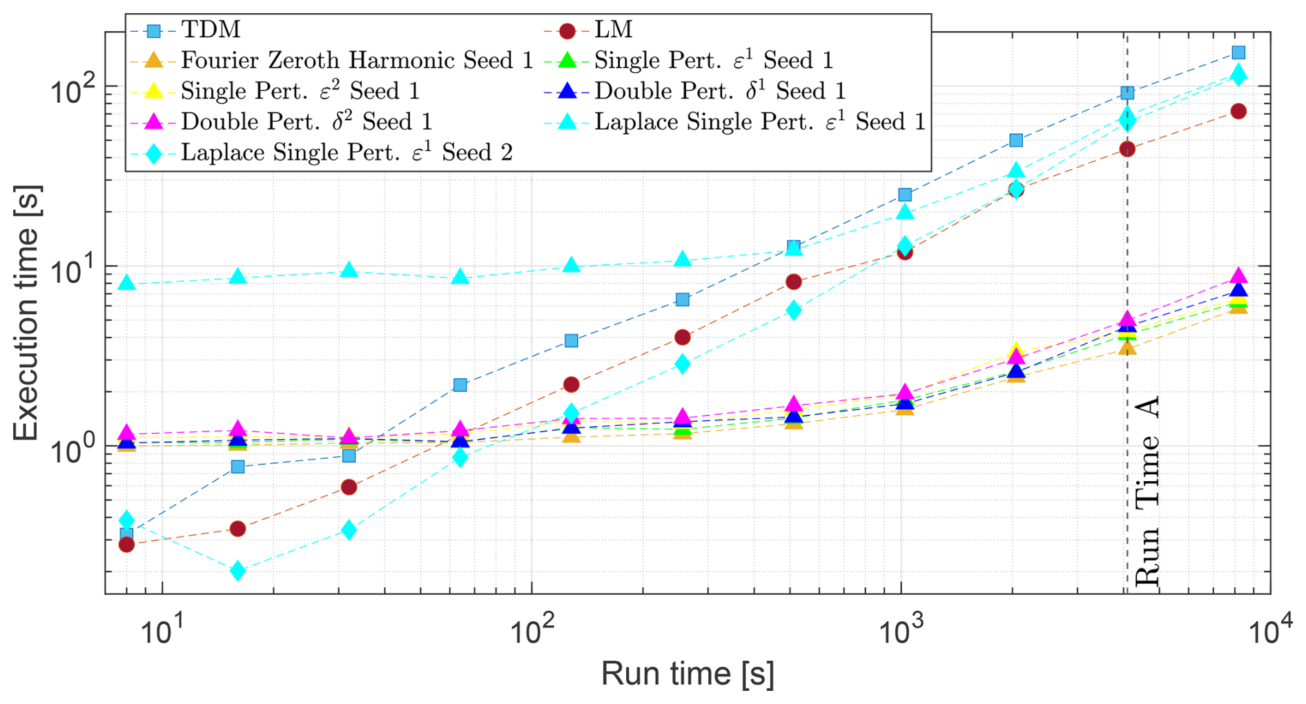
Figure 12 CPU execution time with respect to run time. Results are using the Seed 1 scheme for the Fourier-based fast response methods and the Seed 2 scheme, as well for the Laplace method.

For the TDM, LM, and the Laplace method with the Seed 2, the CPU time is proportional to time simulated with a slope that is very close to 1 in a log-log scale. In contrast, the CPU time for fast response methods has a plateau trend until reaching about 500 s of simulated time. Onward from that point, the fast response method curves become straight, with almost a unit slope and then the CPU time is about 10 times smaller for a first seed simulation than for the LM. Similarly, for the Laplace method with a Seed 1, the CPU time has a plateau value until reaching 1000 s run time, and then onward it has a slope close to 1.

Compared to fast response methods, that run time threshold is highest obviously for the Laplace method with Seed 1 due to its higher computational cost. Before that run time is reached, the Laplace method with a Seed 1 is more computationally expensive in execution time than any other method including the LM and TDM. Also, the Laplace method using the Seed 1 scheme is at all run times less efficient than the LM. Due to the time step looping procedure, the Laplace method is computationally vastly more costly than all other Fourier-based methods. The Laplace method using the Seed 2 scheme is slightly less efficient than the LM at higher run times, otherwise the efficiency is considerably close to the LM results and varies with the same trend. The Laplace single perturbation method is the slowest of the methods we developed, mainly because of the time-looping process used to solve the response and the preliminary symbolic operations needed. A single time loop was tested to solve both the zeroth harmonic q₀ and first-harmonic q₁ responses, but it was found to be slower than using two separate loops to solve each response individually. Additionally, the Fourier-based fast response methods with a Seed 1 are only less efficient than the LM until reaching a run time of 60 s; however, after exceeding that run time threshold, they become more efficient than all other methods.

The CPU time required for a Seed 2 computation using the fast response methods for load Case E is shown in Fig. 13, with both the x and y axes displayed on a log-log scale. There is now a 1:1 ratio between the execution and run time because there are no initialization costs for simulations carried out with a Seed 2. For example, with a run time of 4096 s (run time A in Figs. 12 and 13), the execution time for fast response methods using a single or double perturbation approach, such as the single perturbation approach with a response correction up to the second-order (ε²), is 1638 times faster than the real run time. It is also 36 times faster than the TDM, and 18 times faster than the LM. Since the inverted structural mass matrix can be stored and other operations can be pre-computed for a Seed 1 simulation, the execution time is further reduced by a factor of 2 for a Seed 2 simulation.

Figure 13 CPU execution time for the Seed 2 scheme with respect to run time.

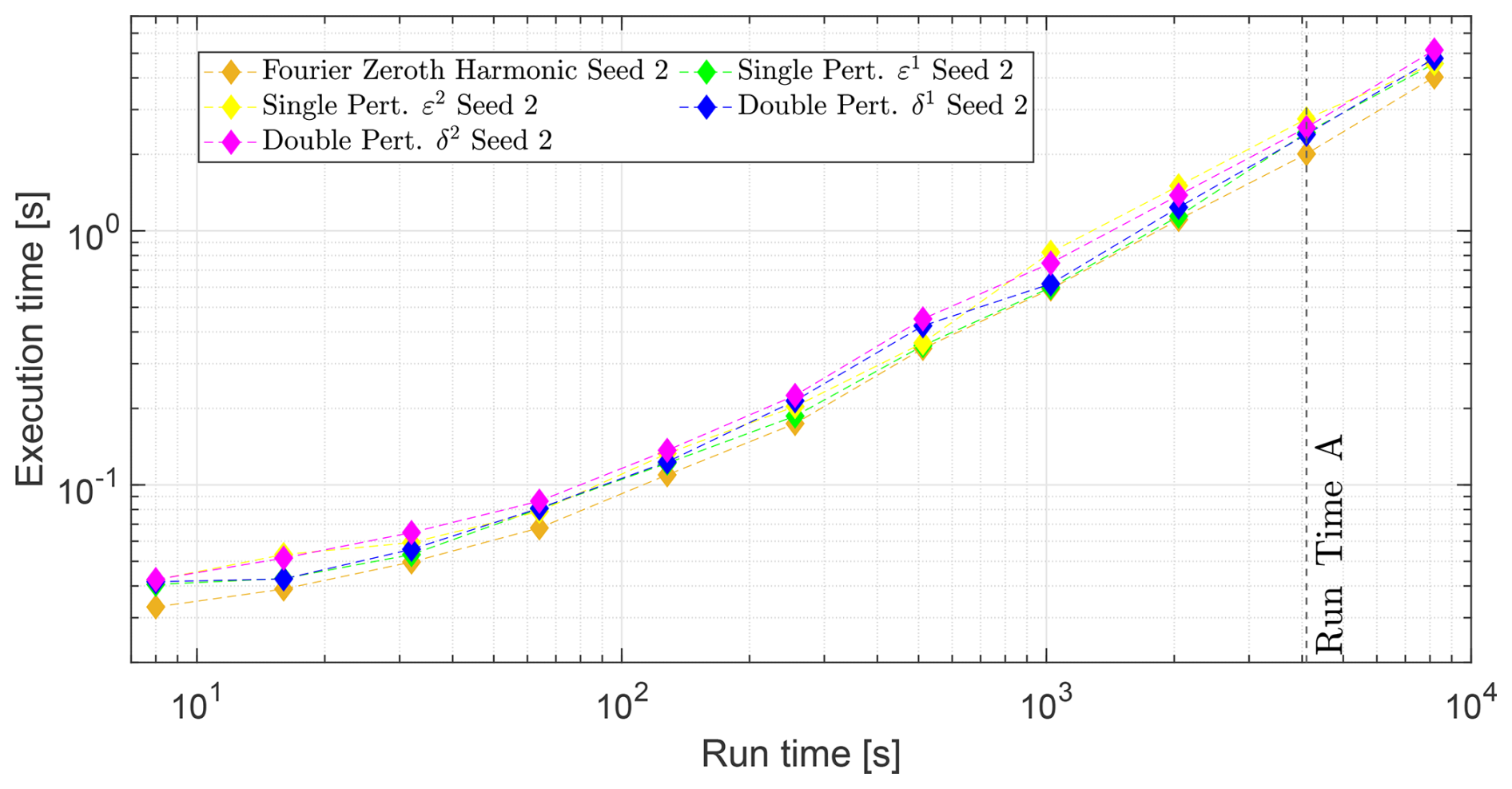
The results for Seeds 1 and 2, in Figs. 12 and 13, indicate, as anticipated, that for both the single and double perturbation results, the single harmonic computation (up to perturbation ε¹ or δ¹) requires less execution time than up to the second harmonic (up to perturbation ε² or δ²).

In the end, the fastest fast response (FFT) method is the zeroth harmonic response contribution only. Due to a lack of accuracy, we find that the best alternative method is the higher-order single perturbation method with a second-order response correction. It is generally faster than the double perturbation method and provides a quasi-identical accuracy. Depending on the load case, a second-order consideration did improve the accuracy, as shown in Fig. 11, and the additional computational cost for adding the second-order correction is small. As an example of accuracy evaluation, one can take into account results again for the run time of 4096 s (run time A). For this scenario, the first-order (up to first-harmonic precision) single perturbation method predicts a result with an accuracy of 3.5 % (Fig. 11) within 2.5 s CPU time. The second-order single perturbation method further improves that accuracy substantially for some load cases, as can be seen in Fig. 11.

Among the various performance metrics analysed, one particularly informative aspect is the overhead or initialization cost incurred by different computational schemes. The results presented in Fig. 14 illustrate the overhead costs that apply when performing simulations according to the Seed 1 computational scheme. These findings complement earlier results by highlighting more the trade-offs between accuracy and computational efficiency.

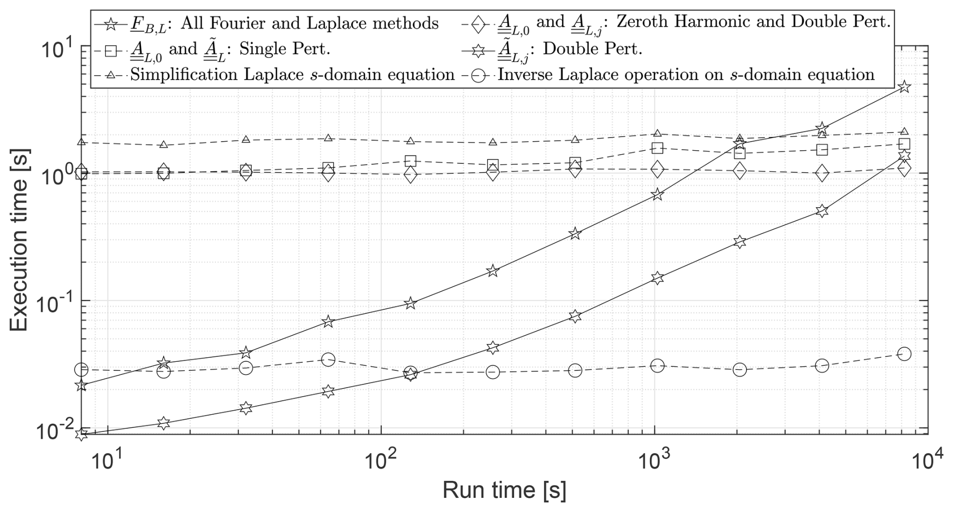
Figure 14 Fast response method overhead costs in terms of execution time versus run time. The methods that require each operation are specified.

For the Laplace method, the highest initialization cost contribution comes from the symbolic simplification procedure of the Laplace s domain Eq. (37), rather than from solving it symbolically.

Another trend that is noticeable in Fig. 14 is that both the forcing time series generation F_B,L(t) and the generation of the double perturbation numerical input forcing term ${\stackrel{\mathrm{̃}}{\mathbf{A}}}_{L,j}\left(t\right)$ are procedures that increase with a unit slope in execution duration with simulation run time. While the total computational cost of A_L,0 and ${\stackrel{\mathrm{̃}}{\mathbf{A}}}_L$ in the single perturbation approach increases with the number of time steps, the growth rate is significantly lower than for the computation of ${\stackrel{\mathrm{̃}}{\mathbf{A}}}_{L,j}\left(t\right)$, owing to the faster evaluation of the matrix ${\stackrel{\mathrm{̃}}{\mathbf{A}}}_L\left(t\right)={\mathbf{A}}_L\left(t\right)-{\stackrel{\mathrm{̃}}{\mathbf{A}}}_{L,\mathrm{0}}$ that grows in size. As expected, the cumulative computation of the matrix A_L,0 and higher harmonic matrices A_L,j via Hill's decomposition remains unaffected by the difference in run time, and it is required for both the zeroth harmonic and the double perturbation methods. Lastly, the Laplace method operations also remain theoretically constant with run time variations, however fluctuations are observed due to the stochastic nature of the runs.

We also evaluated the efficiency of our implementation by measuring the proportion of execution time spent on inverting the structural mass matrix M_S during the generation of the forcing time series F_B,L(t) across all time steps. Our observations showed that it reaches a maximum level of about 10 %. With that plateau value reached as the run time increases, we can consider that only a small proportion of the forcing time series generation F_B,L(t) (Eq. 21) is spent on that operation. This means that this procedure does not require optimization and can remain unchanged without the need to further reduce computational costs.

8 Conclusions

We have developed novel methods in both the frequency and Laplace domains to enable rapid analysis of the aero-elastic behaviour of floating wind turbines. The proposed Fourier-based and Laplace-based perturbation techniques model the system's dynamic response with harmonic accuracy up to the second order. They are intended to serve as practical tools for early-stage design and optimization, providing accurate insights into system behaviour while significantly reducing the computational cost compared to traditional time-domain simulations.

Conventional frequency-domain approaches are unable to treat blade-resolved response effects, since the azimuthal time dependence of the system matrices prevents a direct transformation to the frequency domain. Our model introduced a novel approach by explicitly considering blade-specific rotor loads in both the frequency and Laplace domains, rather than simplifying them to hub-level thrust and torque. Previous studies often represented the equations of motion in state-space form without including the effects of azimuthal blade loading, whereas our formulation incorporates these effects explicitly.

The computationally efficient methods that we formulated were verified under various load cases, including constant inflow, sheared inflow, and stochastic waves and wind. By introduction of a harmonic ordering parameter, the original linear model with a time-varying system matrix was reformulated into a sequence of linear problems with a constant system matrix, suited for solution in the frequency domain. These new methods vary first based on the perturbation approach, which can either be single or double. They can both be evaluated up to a chosen harmonic order. Hereby, higher-order harmonic corrections were shown to improve accuracy at a minimal computational cost. Results demonstrated that zeroth-order approximations were insufficient in cases of strong periodicity, whereas the inclusion of higher harmonics significantly improved fidelity. Further, the Laplace single perturbation method is the slowest among the methods we implemented, primarily due to the time-looping procedure involved in solving the response and the symbolic operations required beforehand.

In terms of computational performance, after initialization costs, the CPU time of the fast response methods scaled proportionally to the simulation time, and achieved speedups of 8 to 10 times relative to the linear baseline. The response accuracy is adjustable via the number of harmonic corrections considered. In the end, an accuracy going up to the second-order perturbation was sufficient to obtain reliable results for all load cases that were studied. The second-order single perturbation offered the best trade-off between speed and accuracy, with an improved speed compared to the double perturbation method. With the linear model used as a reference, a standard deviation relative error below 3.5 % and a largest positive-peak error below 3 % were achieved. Conversely, for the second-order double perturbation method, the error level for the largest response peaks across all load cases and output channels was below 0.5 %. Although the second-order double perturbation method generated a slightly higher accuracy, it required approximately 25 % more CPU time.

The numerical methods that we elaborated on are based on several assumptions and possess few limitations. While the proposed approaches assume a linear system behaviour, which limits the capture of non-linear and transient effects, such assumptions remain appropriate for preliminary design analyses. The difference between the time-domain model and the linear model was quantified to assess the accuracy of the linear approximation. For few load cases, a small difference was observed between the time-domain and linear model results across the time series, PSD, and logarithmic exceedance probability plots, as the time-domain model accounts for non-linear effects resulting from variations in aerodynamic parameters. Additionally, even though frequency-domain analyses are limited in their ability to comprehensively represent transient and non-linear effects, to address this issue, we devised a Laplace-domain method that considers transient response effects from initial conditions and relies on a first-order harmonic approximation. Consequently, it accurately captured the system's dynamic characteristics across most load cases.

The simplicity of the model with only 4 degrees of freedom was chosen to provide a simple and transparent demonstration model for the fast response methods. It thus includes the coupled floater motion and blade aerodynamics with aerodynamic states. Model extensions through the inclusion of additional blade sections, dynamic inflow, tower and blade flexibility, and improved hydrodynamics are possible as future work. To enhance model accuracy, the blade modal representation could be expanded to include edgewise, torsional, and higher-order modes, as well as tower modes, which are currently neglected since the tower is modelled as rigid. Increasing the number of blade sections in the rotor load calculations would yield a more realistic aerodynamic distribution, capturing spanwise variations in turbulence (e.g. from the Mann box). Tower flexibility can be incorporated without difficulty by following the same approach as in the QuLAF model (Pegalajar-Jurado et al., 2018). With regard to floater hydrodynamics, potential improvements, which are also implemented in the QuLAF model, include frequency-dependent radiation damping and added-mass effects, as well as a more detailed representation of hydrostatic stiffness. These effects can be obtained using LPT solvers such as WAMIT, which provide frequency-domain hydrodynamic coefficients for wave excitation, radiation damping, and added mass. Moreover, the present floating wind turbine model formulation readily accommodates the inclusion of additional floater DOFs, particularly for large-volume floaters. Future work could additionally consider incorporating reactive forces from the mooring lines acting on the floater to further refine the floating wind turbine model. Also, the extension to varying rotor speed and control can be made, following the analysis in Pamfil (2025). Finally, the Øye dynamic stall model could be extended to incorporate shed vorticity effects, as accounted for in the Beddoes–Leishman model via Theodorsen's function, but it was used here in its original form for the sake of clarity and demonstration purposes.

However, since the present results demonstrate the feasibility of the novel fast response methods, a much more beneficial future step will be to apply the methods in full aero-elastic models for floating wind turbines. The developed response calculation methods are compatible with state-of-the-art time-domain solvers such as Bladed, OpenFAST, and HAWC2. Thus, they provide a means to obtain model-consistent fast linearized simulation results for use in load case screening, pre-design optimization, and control development.

Appendix A: Velocity triangle

To calculate the aerodynamic load F_l,aero, we quantify the relative velocity V_rel,l by analysing the velocity triangle in Fig. A1.

The integrated normal force F_l,aero on the l^th blade is given by

$$\begin{array}{}\text{(A1)}& F_{l,\mathrm{aero}}=\underset{{\mathrm{F}}_l}{\underbrace{L_l\cos {\mathit{\varphi }}_l}}{L}_{\mathrm{b}}={\displaystyle \frac{\mathrm{1}}{\mathrm{2}}}\mathit{\rho }c{C}_{\mathrm{L},l}\left(\mathit{\alpha }\right)V_{\mathrm{rel},l}^{\mathrm{2}}\cos {\mathit{\varphi }}_l{L}_{\mathrm{b}},\end{array}$$

where ϕ_l is the inflow angle and C_L,l(α) is the lift coefficient as a function of the angle of attack. These aerodynamic properties are evaluated for the airfoil at r=d, which is located at 70 % of the blade's length (d=0.7L_b), and the detailed justification can be found in Sect. 2.3. In this study, it is assumed that the drag and tangential induced velocity contributions are relatively small compared to the lift and axial induction, respectively, and can thus be neglected. While assuming additionally the same inflow angle ϕ_l for the entire blade, we ignore the effects of variation in blade deformation across the blade. Although the inflow angle varies considerably along the blade span, it is evaluated only at a single radial reference position, which is used to compute the aerodynamic forcing for the entire blade. Nevertheless, the assumption of a single inflow angle and angle of attack per blade affects the accuracy of the overall rotor aerodynamic loads. This modelling choice is, however, justified by the objective of developing a floating wind turbine model with fewer DOFs and by the disproportionately high contribution of aerodynamic loads at that blade location – refer to the explanation provided in Sect. 2.3. In Eq. (A1), for linearization purposes, F_l=L_lcos ϕ_l represents the aerodynamic load contribution that dictates the floating wind turbine's dynamics. For the development of the LM, the contributions of the dynamic lift coefficient C_L,l(α), the squared relative wind speed $V_{\mathrm{rel},l}^{\mathrm{2}}=V_{\widehat{n},l}^{\mathrm{2}}+V_{\widehat{t},l}^{\mathrm{2}}$, and the cosine of the inflow angle cos ϕ_l are linearized about the operating point. In contrast, for the TDM, these time-varying quantities are not linearized with respect to the time derivative of the structural DOF vector $\dot{\mathit{x}}$, the dynamic stall separation function DOF f_s,l, or the inflow velocity fluctuation ΔV_0,l. Unlike the LM, the TDM retains non-linear contributions, for example, in the computation of $V_{\mathrm{rel},l}^{\mathrm{2}}$. The TDM accounts for the direct time variation of these aerodynamic parameters by employing their original non-linear definitions.

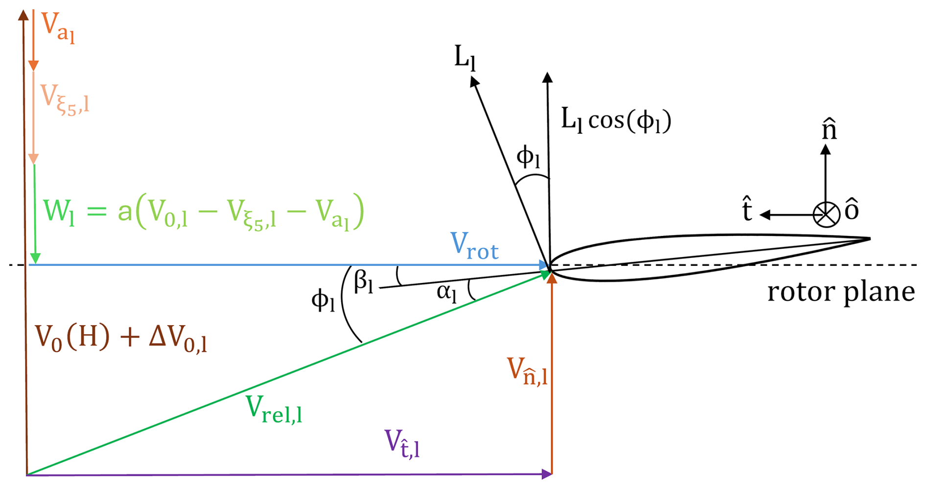
Figure A1 Velocity triangle for the airfoil located at the radial position of r=d on the blade.

As illustrated in Fig. A1, the relative velocity V_rel,l component that is normal to the rotor plane $V_{\widehat{n},l}$ is impacted by a steady-state constant wake induction factor a. Conversely, the velocity tangential to the rotor plane $V_{\widehat{t},l}$ is approximated not to be impacted by a tangential induction wake factor a^′, since this is usually small. Therefore, $V_{\widehat{t},l}$ is equal to the rotational speed itself: $V_{\mathrm{rot}}=-\mathrm{\Omega }d$. Additional relations are found with respect to the inflow angle ϕ_l, the angle of attack α_l, and the twist angle β_l, such as ${\mathit{\varphi }}_l={\mathit{\alpha }}_l+{\mathit{\beta }}_l$ and ${\mathit{\varphi }}_l={\tan }^{-\mathrm{1}}\left(-V_{\widehat{n},l}/V_{\widehat{t},l}\right)$. The velocity normal to the rotor plane is given by $V_{\widehat{n},l}=\left(\mathrm{1}-a\right)\left(V_{\mathrm{0},l}-V_{{\mathit{\xi }}_{\mathrm{5}},l}-V_{{\mathrm{a}}_l}\right)$, where $V_{\mathrm{0},l}=V_{\mathrm{0}}\left(H\right)+\mathrm{\Delta }{V}_{\mathrm{0},l}$, $V_{{\mathit{\xi }}_{\mathrm{5}},l}=\dot{{\mathit{\xi }}_{\mathrm{5}}}\left(H+d\cos {\mathrm{\Psi }}_l\right)$ and $V_{{\mathrm{a}}_l}={\dot{a}}_l{\mathit{\varphi }}_{\mathrm{1}\mathrm{f}}\left(d\right)$. This entails that the squared normal velocity $V_{\widehat{n},l}^{\mathrm{2}}$ can be expanded as

$$\begin{array}{}\text{(A2)}& \begin{array}{rl}& V_{\widehat{n},l}^{\mathrm{2}}={\left(\mathrm{1}-a\right)}^{\mathrm{2}}\left(\underset{\text{steady term}}{\underbrace{V_{\mathrm{0}}^{\mathrm{2}}\left(H\right)}}+\underset{\text{higher-order term neglected}}{\underbrace{\mathrm{2}{\dot{\mathit{\xi }}}_{\mathrm{5}}\left(H+d\cos {\mathrm{\Psi }}_l\right){\dot{a}}_l{\mathit{\varphi }}_{\mathrm{1}\mathrm{f}}\left(d\right)}}\right.\\ & +\underset{\text{higher-order terms neglected}}{\underbrace{{\dot{\mathit{\xi }}}_{\mathrm{5}}^{\mathrm{2}}{\left(H+d\cos {\mathrm{\Psi }}_l\right)}^{\mathrm{2}}+{\dot{a}}_l^{\mathrm{2}}{\mathit{\varphi }}_{\mathrm{1}\mathrm{f}}(d{)}^{\mathrm{2}}}}\\ & +\underset{\text{damping contribution}}{\underbrace{\mathrm{2}\left(V_{\mathrm{0}}\left(H\right)+\mathrm{\Delta }{V}_{\mathrm{0},l}\right)\left(-\dot{{\mathit{\xi }}_{\mathrm{5}}}\left(H+d\cos {\mathrm{\Psi }}_l\right)-{\dot{a}}_l{\mathit{\varphi }}_{\mathrm{1}\mathrm{f}}\left(d\right)\right)}}\\ & \left.+\underset{\text{forcing contribution}}{\underbrace{\mathrm{\Delta }{V}_{\mathrm{0},l}^{\mathrm{2}}+\mathrm{2}{V}_{\mathrm{0}}\left(H\right)\mathrm{\Delta }{V}_{\mathrm{0},l}}}\right),\end{array}\end{array}$$

where $\mathrm{\Delta }{V}_{\mathrm{0},l}=\mathrm{\Delta }{V}_{\mathrm{0},l,\mathrm{shear}}+\mathrm{\Delta }{V}_{\mathrm{0},\mathrm{turb}}$. The damping contribution of the periodic shear inflow velocity variation $\mathrm{\Delta }{V}_{\mathrm{0},l,\mathrm{shear}}$ is considered within the structural damping matrix of the system C_S as an addition of the aerodynamic damping matrix C_A (Eq. 14). The periodicity of $\mathrm{\Delta }{V}_{\mathrm{0},l,\mathrm{shear}}$ (Eq. 11) induces a higher-order harmonic time dependence in the aerodynamic damping matrix C_A (Eq. 15). This time dependence cannot subsequently be eliminated from the state-space system matrix A (Eq. 17) using the Coleman transform, even if the system is formulated in a non-rotating frame. From Eq. (A2), it is evident that both the shear inflow velocity fluctuation $\mathrm{\Delta }{V}_{\mathrm{0},l,\mathrm{shear}}$ and the spatially coherent turbulent fluctuation ΔV_0,turb add to the total velocity variation ΔV_0,l, which in turn influences the forcing term. Also, from Eq. (A2), we neglect the damping contribution of the term $\mathrm{2}\mathrm{\Delta }{V}_{\mathrm{0},\mathrm{turb}}\left(-\dot{{\mathit{\xi }}_{\mathrm{5}}}\left(H+d\cos {\mathrm{\Psi }}_l\right)-{\dot{a}}_l{\mathit{\varphi }}_{\mathrm{1}\mathrm{f}}\left(d\right)\right)$, which is influenced by the spatially coherent velocity fluctuation ΔV_0,turb.

Moreover, partial derivatives involving the inflow angle ϕ_l and a variable of interest, denoted by the ⋅ symbol, i.e. $\frac{\partial {\mathit{\varphi }}_l}{\partial \cdot }$ and $\frac{\partial \cos {\mathit{\varphi }}_l}{\partial \cdot }$, become relevant when linearizing the system equations. They are found to be

$$\begin{array}{}\text{(A3)}& \begin{array}{rl}& {\displaystyle \frac{\partial {\mathit{\varphi }}_l}{\partial \cdot }}={\displaystyle \frac{\mathrm{1}}{-V_{\widehat{t},\mathrm{st}}\left(\frac{V_{\widehat{n},\mathrm{st}}^{\mathrm{2}}}{V_{\widehat{t},\mathrm{st}}^{\mathrm{2}}}+\mathrm{1}\right)}}{\displaystyle \frac{\partial V_{\widehat{n},l}}{\partial \cdot }},\\ & {\displaystyle \frac{\partial \cos {\mathit{\varphi }}_l}{\partial \cdot }}=-{\displaystyle \frac{V_{\widehat{n},\mathrm{st}}}{V_{\widehat{t},\mathrm{st}}^{\mathrm{2}}{\left(\frac{V_{\widehat{n},\mathrm{st}}^{\mathrm{2}}}{V_{\widehat{t},\mathrm{st}}^{\mathrm{2}}}+\mathrm{1}\right)}^{\frac{\mathrm{3}}{\mathrm{2}}}}}{\displaystyle \frac{\partial V_{\widehat{n},l}}{\partial \cdot }},\end{array}\end{array}$$

and are related to the partial derivative of the normal velocity $V_{\widehat{n},l}$ (Pamfil et al., 2025).

Appendix B: Øye dynamic stall model and related studies

The Øye dynamic stall model comprises an equation for the dynamic lift coefficient C_L and for the separation function f_s that influences its behaviour. This model is linearized by applying Eq. (12) first for the dynamic lift coefficient C_L from Øye's model Øye (1991)

$$\begin{array}{}\text{(B1)}& C_{\mathrm{L},l}\left({\mathit{\alpha }}_l,f_{\mathrm{s},l}\right)=f_{\mathrm{s},l}{C}_{\mathrm{L},\mathrm{inv}}\left({\mathit{\alpha }}_l\right)+\left(\mathrm{1}-f_{\mathrm{s},l}\right)C_{\mathrm{L},\mathrm{stall}}\left({\mathit{\alpha }}_l\right).\end{array}$$

In our anterior studies using this dynamic stall model (Pamfil et al., 2025), we have described the linearized terms $\frac{\partial C_{\mathrm{L},l}}{\partial {\mathit{\alpha }}_l}$ and $\frac{\partial C_{\mathrm{L},l}}{\partial f_{\mathrm{s},l}}$, respectively, as

$$\begin{array}{}\text{(B2)}& \begin{array}{rl}& {\displaystyle \frac{\partial C_{\mathrm{L},l}}{\partial {\mathit{\alpha }}_l}}=f_{\mathrm{s},l}{\left.{\displaystyle \frac{\partial C_{\mathrm{L},\mathrm{inv},l}}{\partial {\mathit{\alpha }}_l}}\right|}_{\mathrm{st}}+\left(\mathrm{1}-f_{\mathrm{s},l}\right){\left.{\displaystyle \frac{\partial C_{\mathrm{L},\mathrm{stall},l}}{\partial {\mathit{\alpha }}_l}}\right|}_{\mathrm{st}},\\ & {\displaystyle \frac{\partial C_{\mathrm{L},l}}{\partial f_{\mathrm{s},l}}}={\left.C_{\mathrm{L},\mathrm{inv}}\left({\mathit{\alpha }}_l\right)\right|}_{\mathrm{st}}-{\left.C_{\mathrm{L},\mathrm{stall}}\left({\mathit{\alpha }}_l\right)\right|}_{\mathrm{st}}.\end{array}\end{array}$$

Using the airfoil data from Fig. 3 in our previous investigations (Pamfil et al., 2025), the values of ${\left.\frac{\partial C_{L,\text{inv},l}}{\partial {\mathit{\alpha }}_l}\right|}_{\text{st}}$ and ${\left.\frac{\partial CL,\text{stall},l}{\partial {\mathit{\alpha }}_l}\right|}_{\text{st}}$ are numerically evaluated under steady-state conditions (st) as gradients at the operating angle of attack α_l through the cubic spline interpolation. To quantify the partial derivative $\frac{\partial C_{\mathrm{L},l}}{\partial \cdot }$ for a given variable designated by the ⋅ symbol, the following relation between the angle of attack and inflow angle must be considered:

$$\begin{array}{}\text{(B3)}& {\displaystyle \frac{\partial C_{\mathrm{L},l}}{\partial \cdot }}={\displaystyle \frac{\partial C_{\mathrm{L},l}}{\partial {\mathit{\alpha }}_l}}{\displaystyle \frac{\partial {\mathit{\alpha }}_l}{\partial \cdot }}={\displaystyle \frac{\partial C_{\mathrm{L},l}}{\partial {\mathit{\alpha }}_l}}{\displaystyle \frac{\partial {\mathit{\varphi }}_l}{\partial \cdot }}.\end{array}$$

At last, the ordinary differential equation (ODE) for the dynamic stall separation function f_s,l, ${\dot{f}}_{\mathrm{s},l}=\left(f_{\mathrm{s},\mathrm{static},l}-f_{\mathrm{s},l}\right)/\mathit{\tau }$ is linearized as

$$\begin{array}{}\text{(B4)}& \begin{array}{rl}& {\dot{f}}_{\mathrm{s},l,\mathrm{lin}}=-{\displaystyle \frac{f_{\mathrm{s},l}}{\mathit{\tau }}}+\\ & {\displaystyle \frac{\mathrm{1}}{\mathit{\tau }}}\left({\left.f_{\mathrm{s},\mathrm{static}}\right|}_{\mathrm{s}t}+{\left.{\displaystyle \frac{\partial f_{\mathrm{s},\mathrm{static},l}}{\partial {\mathit{\alpha }}_l}}\right|}_{\mathrm{st}}{\left.{\displaystyle \frac{\partial {\mathit{\varphi }}_l}{\partial {\dot{\mathit{\xi }}}_{\mathrm{5}}}}\right|}_{\mathrm{st}}{\dot{\mathit{\xi }}}_{\mathrm{5}}+\right.\\ & \left.+{\left.{\displaystyle \frac{\partial f_{\mathrm{s},\mathrm{static},l}}{\partial {\mathit{\alpha }}_l}}\right|}_{\mathrm{st}}{\left.{\displaystyle \frac{\partial {\mathit{\varphi }}_l}{\partial {\dot{a}}_l}}\right|}_{\mathrm{st}}{\dot{a}}_l+{\left.{\displaystyle \frac{\partial f_{\mathrm{s},\mathrm{static},l}}{\partial {\mathit{\alpha }}_l}}\right|}_{\mathrm{st}}{\left.{\displaystyle \frac{\partial {\mathit{\varphi }}_l}{\partial \mathrm{\Delta }{V}_{\mathrm{0},l}}}\right|}_{\mathrm{st}}\mathrm{\Delta }{V}_{\mathrm{0},l}\right),\end{array}\end{array}$$

where the time constant is $\mathit{\tau }=\left(\mathrm{4}c\right)/V_{\mathrm{rel},\mathrm{st}}$. The partial derivative ${\left.\frac{\partial f_{\mathrm{s},\text{static},l}}{\partial {\mathit{\alpha }}_l}\right|}_{\text{st}}$ required for the LM is obtained by numerically computing the gradient at the relevant operating angle of attack α_l, based on the airfoil data presented in Fig. 4 from our published paper (Pamfil et al., 2025). As a reminder, the dynamic stall model, like the floating wind turbine model, is employed solely as a demonstration platform to verify the fast response methodology, and is not intended to constitute a central contribution of this study. Øye's dynamic stall model has only a single state and does not account for the separation effect of the vorticity that is shed from the airfoil's trailing edge. This phenomenon is captured analytically by Theodorsen's function, and it is incorporated in the Beddoes–Leishman dynamic stall model (Leishman and Beddoes, 1986). However, we selected the Øye model for this analysis because it simplifies both the implementation and the linearization of the dynamic stall equations within the state-space framework. The validity of the linearization of the Øye dynamic stall model has been verified using the same dynamic model as in our previous published work (Pamfil et al., 2025). Therefore, in Fig. 6 (Pamfil et al., 2025), we compared for both the LM and the TDM the dynamic lift and stall behaviour with a periodic floater pitch M_F excitation. The analysis was carried out at three different operational points near the region of maximum static lift coefficient C_L,static. It demonstrated that overall there is a good agreement between the TDM and LM time series for the angle of attack α and the lift coefficient C_L. A more extensive dynamic stall analysis could compare the behaviour of multiple dynamic stall models. In pursuit of this goal, DNV developed a dynamic stall state-space model within its aero-elastic code Bladed, named IAG (Bangga et al., 2023), in reference to the Institute of Aerodynamics and Gas Dynamics at the University of Stuttgart, reflecting the developer's former affiliation. Their study investigated how the Øye, Beddoes–Leishman, and IAG dynamic stall models respond to varying excitation frequencies in edgewise vibrations of large and flexible wind turbine blades (Bangga et al., 2023), offering valuable insights for blade design. However, choosing the appropriate dynamic stall model is left to the reader, depending on the specific operating conditions, and conducting such a sensitivity study is beyond the scope of this work.

Appendix C: Supplementary statistical analysis

C1 Load Case C: variation of inflow turbulence intensity

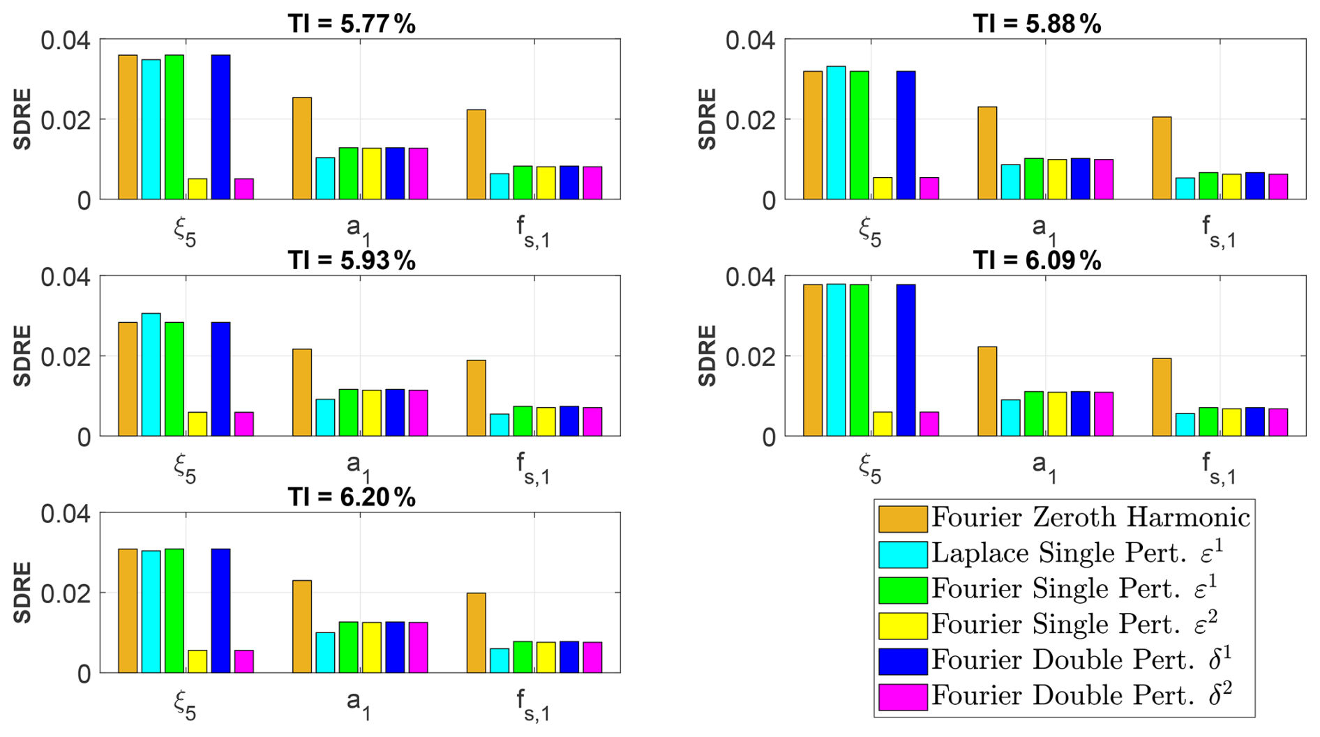
Figure C1 Standard deviation relative error (SDRE) for load Case C turbulence intensity (TI) variations and response channels. The analysed fast response methods are the Fourier zeroth harmonic, as well as the double and single perturbation (pert.) methods.

C2 Load Case D: variation in stochastic hydrodynamic moment with multiple simulation runs

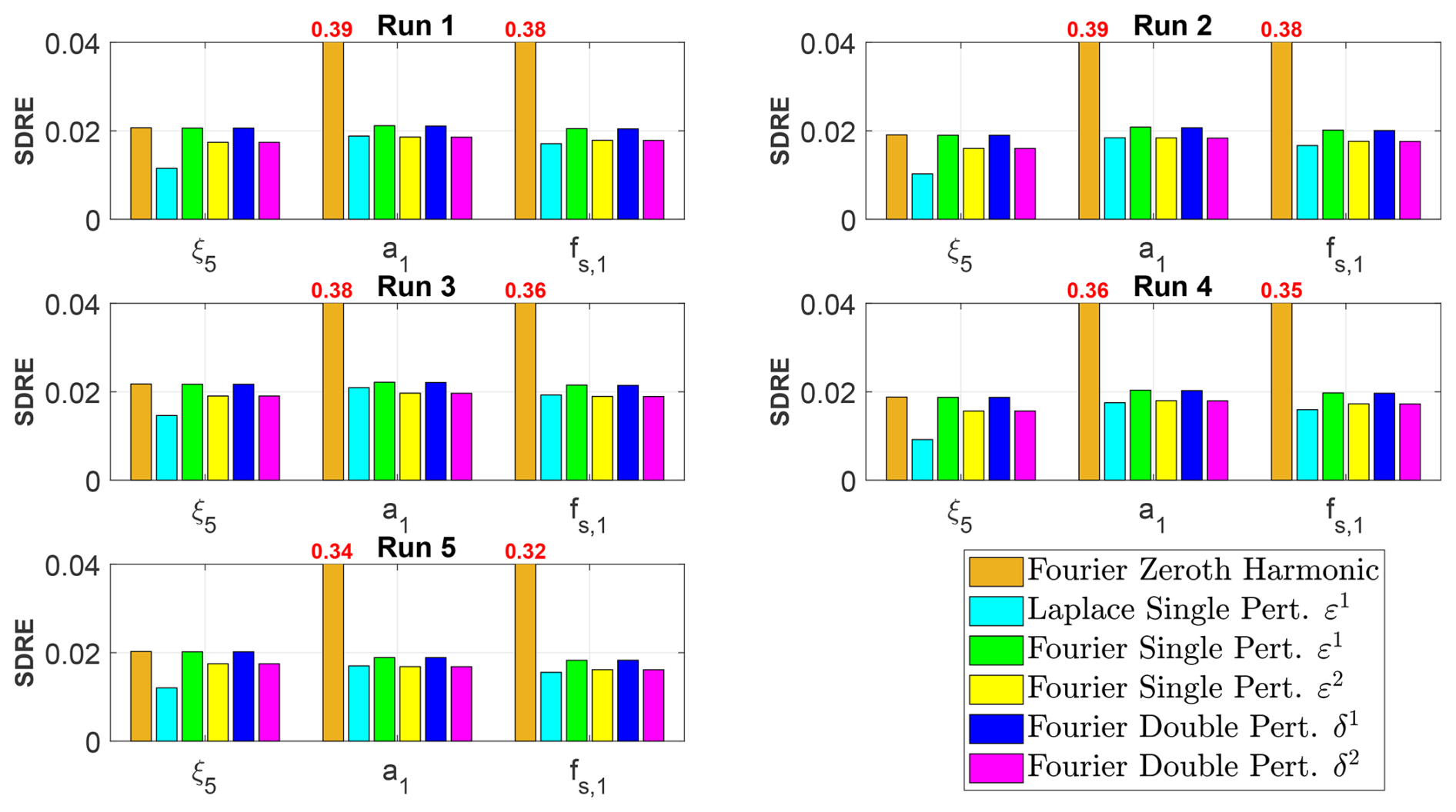
Figure C2 Standard deviation relative error (SDRE) for load Case D multiple runs with different stochastic floater pitch moment and response channels. The analysed fast response methods are the Fourier zeroth harmonic, as well as the double and single perturbation (pert.) methods.

Appendix D: Simulation protocols for Seeds 1 and 2

The simulations protocols are summarized with the following steps for the zeroth harmonic and higher-order perturbation (pert.) methods:

D1 Zeroth harmonic

Seed 1:

• (a)

  Compute F_B,L and store ${\mathbf{M}}_{\mathrm{S}}^{-\mathrm{1}}$ (Eq. 21).

• (b)

  Calculate A_L,0 via Hill decomposition (Eq. 27).

Seed 2:

• (a)

  Compute F_B,L using stored ${\mathbf{M}}_{\mathrm{S}}^{-\mathrm{1}}$.

• (b)

  Use stored A_L,0.

D2 Single pert.

Seed 1:

• (a)

  Compute F_B,L and store ${\mathbf{M}}_{\mathrm{S}}^{-\mathrm{1}}$.

• (b)

  Calculate average A_L,0 and higher first-order harmonic ${\stackrel{\mathrm{̃}}{\mathbf{A}}}_L={\mathbf{A}}_L-{\mathbf{A}}_{L,\mathrm{0}}$ for time series (Eq. 27).

Seed 2:

• (a)

  Compute F_B,L using stored ${\mathbf{M}}_{\mathrm{S}}^{-\mathrm{1}}$.

• (b)

  Use stored A_L,0 and ${\stackrel{\mathrm{̃}}{\mathbf{A}}}_L$.

D3 Double pert.

Seed 1:

• (a)

  Compute F_B,L and store ${\mathbf{M}}_{\mathrm{S}}^{-\mathrm{1}}$.

• (b)

  Calculate A_L,0 and harmonics A_L,j (j>0) via Hill decomposition (Eq. 27).

• (c)

  Compute ${\stackrel{\mathrm{̃}}{\mathbf{A}}}_{L,j}$ for time series using A_L,j (Eq. 27).

Seed 2:

• (a)

  Compute F_B,L using stored ${\mathbf{M}}_{\mathrm{S}}^{-\mathrm{1}}$.

• (b)

  Use stored A_L,0 and ${\stackrel{\mathrm{̃}}{\mathbf{A}}}_{L,j}$.

D4 Laplace single pert.

Seed 1:

• (a)

  Compute F_B,L and store ${\mathbf{M}}_{\mathrm{S}}^{-\mathrm{1}}$.

• (b)

  Simplify symbolic s domain Eq. (36) and compute time solution via inverse Laplace (Eqs. 37 and 38).

Seed 2:

• (a)

  Compute F_B,L using stored ${\mathbf{M}}_{\mathrm{S}}^{-\mathrm{1}}$.

• (b)

  Use stored time-domain solution (Eqs. 37 and 38).

Appendix E: Nomenclature

1f	Blade first flapwise mode
AM	Floater pitch moment amplitude
ASpar	Spar-buoy cylinder cross-sectional area
Awave,j	JONSWAP spectrum wave amplitude
a	Axial induction factor normal to rotor plane
a′	Tangential induction factor
al	Blade deflection amplitude
c	Airfoil chord length
Ca	Hydrodynamic added-mass coefficient
Cm	Hydrodynamic inertia coefficient
CL,inv	Airfoil inviscid flow lift coefficient
CL,l	Airfoil dynamic lift coefficient as blade variable
CL,stall	Airfoil fully separated flow lift coefficient
CL,static	Airfoil static lift coefficient
Dl(r,t)	Blade element distance from the floater basis
DSpar	Spar-buoy diameter
d	Blade reference radial position from the root
fs,l	Dynamic stall separation function as blade variable
$f_{\mathrm{s},\mathrm{static},l}$	Dynamic stall static separation function as blade variable
Fhydro	Hydrodynamic force
Fl,aero	Blade aerodynamic load
g	Gravitational constant
$G{F}_{{\mathrm{a}}_l}$	Generalized aerodynamic blade force
H	Hub height
Hs	JONSWAP spectrum significant wave height
h	Water depth
k(r)	Blade sectional stiffness
kwave,j	Wave number
Lb	Blade length
Ll	Blade lift force per unit length
l	Blade index
M	Combined mass of nacelle and hub
Maero	Aerodynamic moment for floater pitch motion
MF	Floater pitch moment
m(r)	Blade mass per unit length
Nb	Number of blades
Ns	Number of states, or the system dimension
pl(r,t)	Blade rate of change of angular momentum
r	Blade radial position from the root
t	Time
ti	Time step of index i
Tp	JONSWAP spectrum peak period
ul(r,t)	Blade deflection
V0(H)	Rotor constant inflow at hub height
Vr	Rated wind speed

Vrel,l	Airfoil relative velocity as blade variable
${\widehat{A}}_l(r,t)$	Blade element acceleration tracked in ${\widehat{x}}^{\prime }-{\widehat{y}}^{\prime }$ coordinate system
${\widehat{D}}_l(r,t)$	Blade element position tracked in ${\widehat{x}}^{\prime }-{\widehat{y}}^{\prime }$ coordinate system
${\widehat{V}}_l(r,t)$	Blade element velocity tracked in ${\widehat{x}}^{\prime }-{\widehat{y}}^{\prime }$ coordinate system
${\widehat{x}}_{\mathrm{Bot}}$	Spar-buoy submerged underwater draft
αl	Airfoil angle of attack as blade variable
βl	Airfoil twist angle as blade variable
γ	JONSWAP spectrum enhancement factor
δn	Perturbation of order n
δk	Logarithmic decrement for a kth degree of freedom
δal(t)	Blade displacement amplitude virtual work
δul(r,t)	Blade displacement virtual work
δξ5(t)	Floater pitch angle virtual work
ϵwave,j	Wave spectrum stochastic phase shift
ζk	Damping ratio for a kth degree of freedom
μ	Structural stiffness matrix scaling factor for Rayleigh damping characterization
νshear	Wind shear exponent
Ω	Constant rotational speed
ΩM	Floater pitch moment excitation frequency
ω1f	Blade first flapwise mode natural frequency
ωwave	JONSWAP spectrum wave frequency
${\mathit{\omega }}_{{\mathit{\xi }}_{\mathrm{5}}}$	Floater pitch natural frequency
ϕ1f	Blade first flapwise mode shape
ϕl	Airfoil inflow angle as blade variable
Ψl(t)	Blade azimuthal angular position
ρ	Air density
ρwater	Water density
τ	Dynamic stall time constant
τhydro	Hydrodynamic moment
ξ5	Floater pitching angle
ΔV0,l	Blade inflow velocity variation
$\mathrm{\Delta }{V}_{\mathrm{0},l,\mathrm{shear}}$	Blade shear inflow velocity variation
ΔV0,turb	Rotor spatially coherent turbulence inflow velocity variation
A	State-space system matrix
AL	Linear model system matrix
AT	Time-domain model system matrix
CA	Aerodynamic damping matrix
CS	Structural damping matrix
I	Identity matrix
KS	Structural stiffness matrix
MS	Structural mass matrix
0	Zero vector or zero matrix
FB	State-space forcing input vector
FB,L	Linear model state-space forcing vector
FB,T	Time-domain model state-space forcing vector
FL	Linear model forcing vector
FT	Time-domain model forcing vector

q	State vector
x	Structural degrees of freedom vector
lin	Linearized variable
st	Steady value of variable
ANOVA	Analysis of variance
DOF	Degree of freedom
EOM	Equation of motion
FFT	Fast Fourier transform
FOWT	Floating offshore wind turbine
IAG	Institute of Aerodynamics and Gas Dynamics
iFFT	Inverse fast Fourier transform
LM	Linear model
LPT	Linear potential theory
LTI	Linear time invariant
ODE	Ordinary differential equation
PSD	Power spectral density
QuLAF	Quick load analysis of floating wind turbines
RAFT	Response amplitudes of floating turbines
RK4	Fourth-order Runge–Kutta
SDRE	Standard deviation relative error
SLOW	Simplified Low-Order Wind turbine
TDM	Time-domain model
TI	Turbulence intensity
WAMIT	Wave analysis MIT