The impact of sea breezes on offshore wind energy resources in Australia

Future projected increases in offshore wind energy in Australia means that it is important to understand variability in wind resources. This includes the potential diurnal variation of wind, along with its co-variability with known diurnal variations of energy demand and supply. A key mechanism for diurnal variations in coastal near-surface winds is the sea breeze, which is driven by differential land–sea surface heating during the day. Here, a new dataset characterising the sea breeze as a frontal object, derived from a km-scale reanalysis, is used to analyse the impact of the sea breeze on diurnal variations of wind energy resources during 1979–2024. This analysis is performed over eight potential offshore wind areas in southeastern and southwestern Australia during the summer. On days with a sea breeze object, there tends to be more potential wind energy resources available in coastal and offshore wind areas during the afternoon, although there may also be late-morning lulls due to the sea breeze opposing the existing prevailing winds. In addition, days with a sea breeze correspond to higher operational regional energy demand on average, due to warmer air temperatures over the land, while the peak in potential wind energy occurs with similar timing to peak demand. Finally, due to the role of the prevailing wind direction in sea breeze formation, there is an anti-correlation in occurrences between opposite-facing coastlines. These results have implications for energy system planning and suggest that offshore wind farm development on a diverse set of coastlines should be encouraged in Australia.

1 Introduction

Global offshore wind energy is growing rapidly, with 83 GW of installed capacity as of 2024 (Global Wind Energy Council, 2025). Although there are currently no offshore wind farms operational in Australia, it is projected to grow into the future, with Australian state government targets of 9 GW by 2050 (Australian Energy Market Operator, 2024). To help in understanding the potential impacts on energy system reliability, it is important to understand variability in wind resources in offshore coastal areas. Wind energy resources in Australia can vary on a range of time scales, from diurnal to multi-year (Vincent and Dowdy, 2024), including periods of low wind that could lead to potential shortfalls in supply (Richardson et al., 2023). Diurnal variations in wind energy resources are particularly important, given that there are also large diurnal variations in both energy demand and existing supply (for example, Mulder, 2014; Simshauser and Wild, 2025). Previous studies have suggested that diurnal wind variations could align well with diurnal peaks in energy demand (Pickering et al., 2020; Vincent et al., 2025).

In coastal areas, the sea breeze is a dominant mode of diurnal wind variability. It is the result of differential surface heating between the land and sea during the day, and is often described as a thermally direct circulation, which has an onshore surface branch with rising air over the land and an offshore branch aloft with descending air over the sea (Markowski and Richardson, 2010). The differential surface temperature forcing can also be influenced by small-scale variations in land-use types, such as due to the presence of cities along the coastline (Wang et al., 2017). The onshore surface branch of the sea breeze tends to form a front ahead of the maritime air mass (the sea breeze front) that can propagate several hundreds of kilometres onshore as a density current (Clarke, 1983; Simpson, 1999; Bao et al., 2023). Meanwhile, the sea breeze circulation can influence the offshore surface wind field, and this has been shown to impact offshore wind energy potential in several regions already, including in the North Sea (Steele et al., 2015) and the United States (Xia et al., 2022). Sea breezes may also occur at the same time as coastal low-level jets (McCabe and Freedman, 2023). These jets can be forced by land–sea temperature differences on synoptic scales and/or topographic blocking (Chao, 1985; Colle and Novak, 2010). In regions equator-ward of 30° latitude, the offshore extent of the sea breeze system can also be influenced by inertia-gravity waves that propagate away from the region of diurnal coastal heating (Rotunno, 1983; Short et al., 2019).

Sea breeze occurrences and their intensity can also be influenced by the prevailing background wind conditions. For example, prevailing onshore winds are typically considered to be unfavourable for sea breeze formation (Frysinger et al., 2003; Masouleh et al., 2019; Xia et al., 2022). Sea breezes have been observed to occur in such conditions but with a weaker front (Reible et al., 1993). In contrast, along-shore prevailing winds with the land to the right (in the Southern Hemisphere) can lead to “corkscrew” sea breezes, and prevailing winds with the land to the left can lead to “backdoor” sea breezes (Miller et al., 2003, with the inverse occurring in the Northern Hemisphere). Corkscrew sea breezes are often observed to have stronger surface wind speeds compared with backdoor sea breezes, as well as so-called “pure” sea breezes that occur with prevailing winds that are directly offshore (Steele et al., 2015). Miller et al. (2003) suggest that corkscrew sea breezes are more intense due to the gradient in surface friction over land and sea surfaces. This creates differential and divergent ageostrophic wind components over the land and sea towards synoptic-scale low-pressure regions (to the right in the Southern Hemisphere), both acting in the same direction as the onshore sea breeze flow. Steele et al. (2015) demonstrated that these different sea breeze types can have varying impacts on offshore wind energy potential. In addition, the prevailing wind speed and direction have been shown to influence the offshore and onshore extent of the sea breeze (Arritt, 1989; Rafiq et al., 2020; Finocchio et al., 2025).

Here, we investigate the impact of sea breezes on the diurnal cycle of wind energy resources for several potential offshore wind areas in southeastern and southwestern Australia. This is done using a new dataset of sea breeze objects derived from an atmospheric reanalysis, based on a diagnostic of sea breeze fronts presented by Brown et al. (2026). Typically, previous studies have identified sea breezes for individual coastal sites based on local characteristics, with the approach here representing a more general and robust method for detection, allowing for consistent analysis over a broader region. Sea breeze objects are derived from a km-scale atmospheric reanalysis over Australia for a 46-year period. These km-scale models are able to more accurately resolve mesoscale sea breeze processes over complex coastlines, compared with coarser models that are more suited to representing the large-scale processes conducive to sea breeze formation (Bergemann et al., 2017; Cafaro et al., 2019).

Sea breeze objects are used to investigate the seasonal cycle and spatial distribution of sea breezes over the broad region of southwest and southeast Australia. Then, the diurnal cycle of wind energy capacity factors are calculated over specific wind energy regions for days with a sea breeze object and are compared with other days to quantify the wind resource associated with the sea breeze. For simplicity, the latter analysis is presented for the austral summer period (December–February), given that this time of year is when sea breezes are more likely to occur due to relatively intense daytime heating of the land. The diurnal cycle in wind energy is compared with regional operational energy demand for each offshore wind area as a qualitative assessment of the value of the potential energy resource related to sea breezes. In addition, we also consider the co-variability of sea breezes across different offshore wind zones as an important consideration for optimising energy systems (Gunn et al., 2023).

2 Data and methods

2.1 Sea breeze objects

A frontogenesis method is used as a diagnostic of sea breeze fronts from atmospheric model output, following a method outlined by Brown et al. (2026). Diagnostics of frontogenesis can identify areas of growth in the frontal boundary between relatively cool, moist maritime air and dry, warm terrestrial air (Keyser et al., 1988; Kraus et al., 1990). Positive frontogenesis values indicate regions where the gradient in a scalar quantity is increasing due to deformation in the horizontal flow. In the case of sea breezes, specific humidity (q) is chosen as the scalar quantity, referred to as “moisture frontogenesis”. The frontogenesis formulation is in the form of Pettersen (1956):

$$\begin{array}{}\text{(1)}& F={\displaystyle \frac{\mathrm{1}}{\mathrm{2}}}\left|{\mathrm{\nabla }}_{h}q\right|[D_{\mathrm{total}}\times \cos (\mathrm{2}B)-\mathit{\delta }],\end{array}$$

where D_total is the total deformation of the surface wind field, B is the angle between the axis of dilatation (the axis along which the stretching of the air is most rapid) and the isopleths of q, and δ is the divergence of the surface wind field. Deformation is defined as $D_{\mathrm{total}}=\sqrt{D_{\mathrm{stretch}}^{\mathrm{2}}+D_{\mathrm{shear}}^{\mathrm{2}}}$, where $D_{\mathrm{stretch}}=\mathrm{d}u/\mathrm{d}x-\mathrm{d}v/\mathrm{d}v$ is the stretching deformation and $D_{\mathrm{shear}}=\mathrm{d}v/\mathrm{d}x+\mathrm{d}u/\mathrm{d}v$ is the shearing deformation. F is quoted here in units of grams per kilogram per 100 km per 3 h (g kg⁻¹ (100 km)⁻¹ (3 h)⁻¹), for convenience.

The sea breeze identification method consists of calculating the moisture frontogenesis diagnostic using hourly data over 1979–2024, from the Bureau of Meteorology Atmospheric Regional Reanalysis for Australia version 2 (BARRA2; Su et al., 2025). The BARRA2 reanalysis system includes a regional model run over the broader Australasia region with 12 km horizontal grid spacing (BARRA-R2) and a downscaled model run over Australia with 4.4 km horizontal grid spacing (BARRA-C2). The 4.4 km BARRA-C2 is used here to broadly represent the mesoscale structure of the sea breeze. Coarser models such as the regional BARRA-R2 model may not capture the correct structure and evolution (Cafaro et al., 2019; Brown et al., 2026).

Following Brown et al. (2026), surface wind and moisture variables from BARRA-C2 are smoothed in the spatial dimension prior to calculating frontogenesis to remove small-scale moisture gradients. Smoothing is performed using a rolling weighted average, with a Gaussian weighting function having a standard deviation of 2 grid points. This smoothing method was chosen based on its performance for individual sea breeze cases, where it was judged to remove a sufficient amount of small-scale gradients while retaining the dominant sea breeze signal. However, in some cases, this smoothing could potentially remove sea breezes forced by land masses with small spatial scales. For a further discussion of this smoothing, as well as quantitative tests for the sensitivity of sea breeze object identification to the amount of smoothing, the reader is referred to Brown et al. (2026).

For calculating frontogenesis, 10 m u and v winds are used, as well as surface specific humidity (at a height of 1.5 m). A mask of candidate sea breeze objects is then created by taking exceedances of frontogenesis over a threshold value. A threshold value of 16.1 g kg⁻¹ (100 km)⁻¹ (3 h)⁻¹ is used (1.5 $\times {\mathrm{10}}^{-\mathrm{8}}$ g kg⁻¹ m⁻¹ s⁻¹), corresponding to the 99.5th percentile of F over Australia, calculated from 6 months of January–February periods (Brown et al., 2026). This percentile value was chosen based on the performance of the method for individual cases, allowing for the correct identification of sea breezes while removing other weak non-sea-breeze fronts. Brown et al. (2026) note that the use of a lower threshold (99th percentile) results in too many moisture fronts identified over the land throughout the day. In contrast, a higher threshold (99.9th percentile) results in similar object statistics over a 6-month period but with fewer objects identified.

Next, a series of filters are applied to the candidate sea breeze mask, intended to remove non-sea-breeze fronts. These filters include conditions on the morphology of the objects, as well as constraints on object-averaged physical variables. The morphological filters ensure that objects are at least 12 pixels in size, oriented with a similar angle as the nearby coastline (within a 45° tolerance) and have an aspect ratio greater than 2, with the expectation that sea breeze objects will be longer in the along-shore direction compared with the cross-shore direction. They must also have a positive land–sea temperature difference, a positive onshore wind speed averaged over the object and a temporal increase in specific humidity. These filters are discussed in more detail in the Supplement (Sect. S1). For further details on the sea breeze identification method, the reader is referred to Brown et al. (2026).

As a way of evaluating the sea breeze identification method, we have compared the seasonal cycle in “sea breeze front days” (see Sect. 2.2 for definition) with three previous studies in different regions of Australia (Masselink and Pattiaratchi, 2001; Pazandeh Masouleh et al., 2016; Soderholm et al., 2017). These comparisons are shown in Sect. S2 of the Supplement. The number of sea breeze front days defined using the methods here are similar to these previous studies, with a broadly similar seasonal cycle, despite the very different methods and periods used. This provides confidence in the use of the methods described here.

However, it should be kept in mind that misclassification of other fronts and circulations as sea breezes are possible. This includes convective cold pools, upslope mountain flows, frictional convergence at the coast, synoptic fronts and dry lines, with separation of these different circulations sometimes not possible. In addition, the smoothing and thresholds applied in the object identification methods may result in the exclusion of small-scale or weak sea breeze fronts. This is discussed further in Sect. 3.2.

2.2 Offshore wind areas and sea breeze front days

The impact of the sea breeze on wind energy resources is analysed for eight different potential offshore wind areas in southeastern and southwestern Australia (Fig. 1). These areas are either high priority for offshore wind farm development, as declared by the Australian Government (Department of Climate Change, Energy, the Environment and Water, 2024), or expected areas for development as part of future energy system planning (Australian Energy Market Operator, 2024). However, there are currently no installed offshore wind farms in Australia.

The areas are described as follows. In southwestern Australia, the Bunbury offshore wind area is considered and split into two, referred to here as “Bunbury Nearshore” and “Bunbury Offshore” according to the relative distance from the coast (Fig. 1a). In southeastern Australia, there are six offshore areas (Fig. 1b), including two off the subtropical east coast near the city of Sydney in the state of New South Wales (Newcastle and Illawarra). There are two areas in the Bass Strait between mainland Australia and the island of Tasmania to the south (Gippsland and Tasmania), and two to the west off the coast of the states of Victoria (Southern Ocean) and South Australia (South Australia).

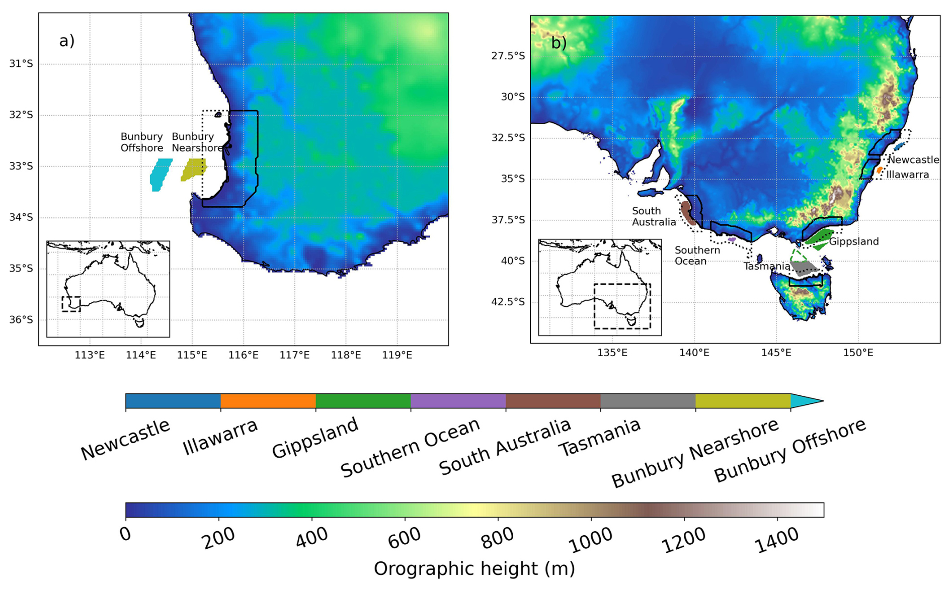
Figure 1 Map of offshore wind areas and adjacent coastal land areas in (a) southwestern Australia and (b) southeastern Australia. Each of the eight offshore wind areas are shown with a different colour and are labelled. The seven adjacent coastal areas over the land, used to define sea breeze front days, are shown with solid black contours. Coastal areas over the sea are shown with a dotted black line, used in the definition of land–sea temperature contrast. Both the onshore and offshore coastal zones extend to a maximum of 50 km inland and offshore, respectively. For the Gippsland offshore wind region (green contours), the official region declared by the Australian Government includes a portion in the middle of Bass Strait (dotted green region). However, this portion is removed from analysis here due to the lack of a clear adjacent coastline for defining sea breeze front days. Topographic data from BARRA-C2 are shown with shading.

For each offshore wind area, a sea breeze front day (SBF day) is defined by the occurrence of a sea breeze object over the adjacent coastal land area, between 10:00 and 21:00 Australian Eastern Standard Time (AEST, UTC+10) for areas in southeastern Australia and between 10:00 and 21:00 Australian Western Standard Time (AWST, UTC+8) for areas in southwestern Australia. These time zones (AEST and AWST) will sometimes be collectively referred to as “local standard time” for convenience. Coastal land areas for defining SBF days were subjectively chosen, intended to represent regions where the sea breeze could potentially influence surface winds in the offshore wind areas, with each area shown in Fig. 1. Despite sea breeze objects being mainly identified over the land (see object occurrence maps in Sect. 3.1), surface winds over adjacent oceans can be influenced due to the broader circulation (Rafiq et al., 2020; Finocchio et al., 2025). The coastal land areas were restricted spatially, such that the extent of each area is within 50 km of the coastline. This limits the potential impacts of steep topography near some of the coastal land areas on sea breeze identification (Fig. 1b), where the influence of upslope mountain breezes can become confounded with the sea breeze. Although there are eight offshore wind areas, as described previously, there are only seven unique coastal land areas due to the two Bunbury areas having the same adjacent coastline (Fig. 1a). For the Gippsland offshore wind area, situated off the coast of the state of Victoria, part of the official declared area near the middle of the Bass Strait (see green dotted contour line in Fig. 1b) has been ignored in subsequent analysis due to the lack of a clear adjacent coastline for defining sea breeze front days.

In the Results section, the seasonal cycle of SBF days for the different coastal areas are reported, as well as the average wind energy capacity factor on SBF days for each offshore wind area compared with “other days”. These other days are defined as days without a sea breeze object identified in each coastal land area. These days may include other diurnally varying wind processes that could resemble sea breezes, such as the daytime vertical mixing of winds from aloft or upslope mountain breezes. In addition, these other days could include weak coastal circulations that do not form a sea breeze front of sufficient strength to be identified by our methods.

2.3 Land–sea temperature difference

To help explain variability in sea breeze front days in each coastal region, we calculate the land–sea temperature difference (T_land−T_sea) as a measure of sea breeze forcing. For the land temperature (T_land), we consider hourly near-surface air temperature from BARRA-C2 averaged over the coastal land areas in Fig. 1. For the sea temperature (T_sea), we consider hourly BARRA-C2 near-surface air temperatures averaged over the coastal ocean areas adjacent to each coastal land area, shown by the dotted black lines in Fig. 1. The coastal land and ocean areas for calculating T_land and T_sea are restricted to be within 50 km of the coastline. Hourly T_land−T_sea values for each area are then resampled to a daily time series by taking the maximum for each day in local standard time. The monthly mean daily maximum T_land−T_sea is presented in the Results section.

Although this approach provides a broad measure of sea breeze forcing, there are uncertainties around defining the land–sea temperature difference, with various approaches adopted by previous studies. This includes regionally averaging temperatures in the cross-shore and/or along-shore directions (Cafaro et al., 2019; Xia et al., 2022; Huang et al., 2025), using single model grid values at fixed distances (Bergemann et al., 2017; Arrillaga et al., 2020) and using observed point values at fixed distances in the onshore and offshore directions, such as 300 m, 20 km or 30 km (Borne et al., 1998; Frysinger et al., 2003; Azorin-Molina et al., 2011), as well as directly on the shoreline (Assireu et al., 2024). Threshold values of T_land−T_sea are often used as a condition for sea breeze development, but there is a lack of consensus on this threshold, with values such as 0, 1.5 and 3 °C used in the literature (Borne et al., 1998; Azorin-Molina et al., 2011; Xia et al., 2022). In the current study, a regional average is used considering model grid points within 50 km of the coastline, rather than individual points. This is intended to capture the broad mesoscale sea breeze forcing, ignoring small-scale surface temperature variability. This is acknowledged as a potential uncertainty, with small-scale temperature gradients shown previously to impact sea breeze characteristics (e.g. Wang et al., 2017).

2.4 Wind power model and energy demand data

Wind energy resources are quantified using capacity factors calculated from hourly BARRA-C2 wind speeds at 100 m above the surface. This is done over the same 1979–2024 period as for the sea breeze objects. The BARRA-C2 wind speeds are calculated from u and v wind components, which have been provided at a height of 100 m in BARRA-C2 by logarithmically interpolating the original model-level data. This interpolation is intended to be suited to the approximate logarithmic wind profile near the surface but does ignore the impact of stability on the wind profile. There are approximately eight model levels in the lowest 200 m, although the exact heights of these levels vary with the model orography.

Capacity factors are based on the International Energy Agency (IEA) offshore 10 MW reference wind turbine (Bortolotti et al., 2019). The power curve data for the IEA reference turbine are provided by the National Laboratory of the Rockies, with a cut-in wind speed of 3 m s⁻¹, a cut-out wind speed of 25 m s⁻¹ and rated power reached at 11 m s⁻¹. Power curve data are made available at intervals ranging from 0.5 to 1.0 m s⁻¹ (National Laboratory of the Rockies, 2026), with a cubic spline interpolation used to map BARRA-C2 wind speeds onto the curve (Virtanen et al., 2020). The power curve does not account for any hysteresis near cut-out wind speeds. Further details on the IEA reference turbine can be found at https://natlabrockies.github.io/turbine-models/IEA_10MW_198_RWT.html (last access: 22 April 2026). It is noted that this approach using a power curve for a single turbine does not account for wake effects in a wind farm. This would likely reduce the energy produced by an operational wind farm relative to the values reported here.

Capacity factors are presented for different times of the day, separately for sea breeze front days and other days, both as spatial maps and spatial averages over each offshore wind area. Capacity factors will mostly be shown for the austral summer period (December–February) when sea breezes are more likely to occur due to relatively intense daytime heating of the land, with results for other seasons shown in the Supplement (Sect. S3).

It should be kept in mind that there are uncertainties in estimating wind energy potential from the BARRA-C2 reanalysis. Although the regional version of BARRA (BARRA-R2) has demonstrated improvements over other reanalysis models in simulating wind speeds at turbine hub height, including ERA5 and MERRA-2 (Cowin et al., 2023; Palmer et al., 2025), BARRA-C2 has not yet been thoroughly evaluated. In addition, there are significant limitations in using wind speeds from gridded models for representing wind energy at the turbine scale (Davidson and Millstein, 2022). Therefore, the capacity factors reported here should mostly be interpreted in terms of the relative contribution from sea breezes, with potential biases in the absolute values reported.

To help assess the potential value of offshore wind energy resources related to sea breezes, the average daily cycle in regional operational energy demand is compared with capacity factors for each offshore area on sea breeze front days and other days. Energy demand data for the eastern regions are obtained from the Australian Energy Market Operator (AEMO) via the NEMOSIS software package (Gorman et al., 2018). The data are provided regionally for each Australian state in the National Energy Market (NEM). The capacity factor for each offshore wind region is compared with demand data for the Australian state in closest proximity. The NEM demand data are provided at intervals of 5 min and are subset to hourly intervals corresponding to the BARRA-C2 data. Demand data for the Australian state of Western Australia (including the Bunbury areas) are obtained directly from AEMO at 30 min intervals and are similarly subset to hourly intervals (https://www.aemo.com.au/energy-systems/electricity/wholesale-electricity-market-wem/data-wem/market-data-wa, last access: 11 November 2025). Following Richardson et al. (2025), each energy demand dataset is restricted to the period of 2010–2019 to remove potential impacts of the COVID-19 pandemic from 2020 onwards. As for the capacity factors discussed above, diurnal energy demand profiles are considered for the austral summer (December–February).

3 Results

3.1 Spatial and seasonal variations in sea breeze occurrences

The spatial distribution of sea breeze object occurrence frequency is shown seasonally for southeastern Australia in Fig. 2 and for southwestern Australia in Fig. 3, in terms of the average number of days with an object identified. Sea breeze objects are identified most frequently near the coastline over the land due to the characterisation of the sea breeze as a front (Sect. 2.1). The diurnal inland movement of the sea breeze front can be seen through the gradient in object occurrence frequency, particularly in relatively flat regions such as the western part of eastern Australia (Fig. 2) or in southwestern Australia (Fig. 3). In these regions, objects can be seen as far as 300 km inland on average, as defined by an occurrence frequency contour of 2 d per season. The sea breeze front can propagate further than this (Clarke, 1983) but is not seen here due to the dissipation of moisture gradients to the point where the strength of the front falls below the selected identification threshold (see Sect. 2.1). Although sea breeze objects are identified almost exclusively over the land, the influence of the broader sea breeze circulation on the boundary layer wind field is expected to extend some distance offshore (e.g. Rafiq et al., 2020; Finocchio et al., 2025).

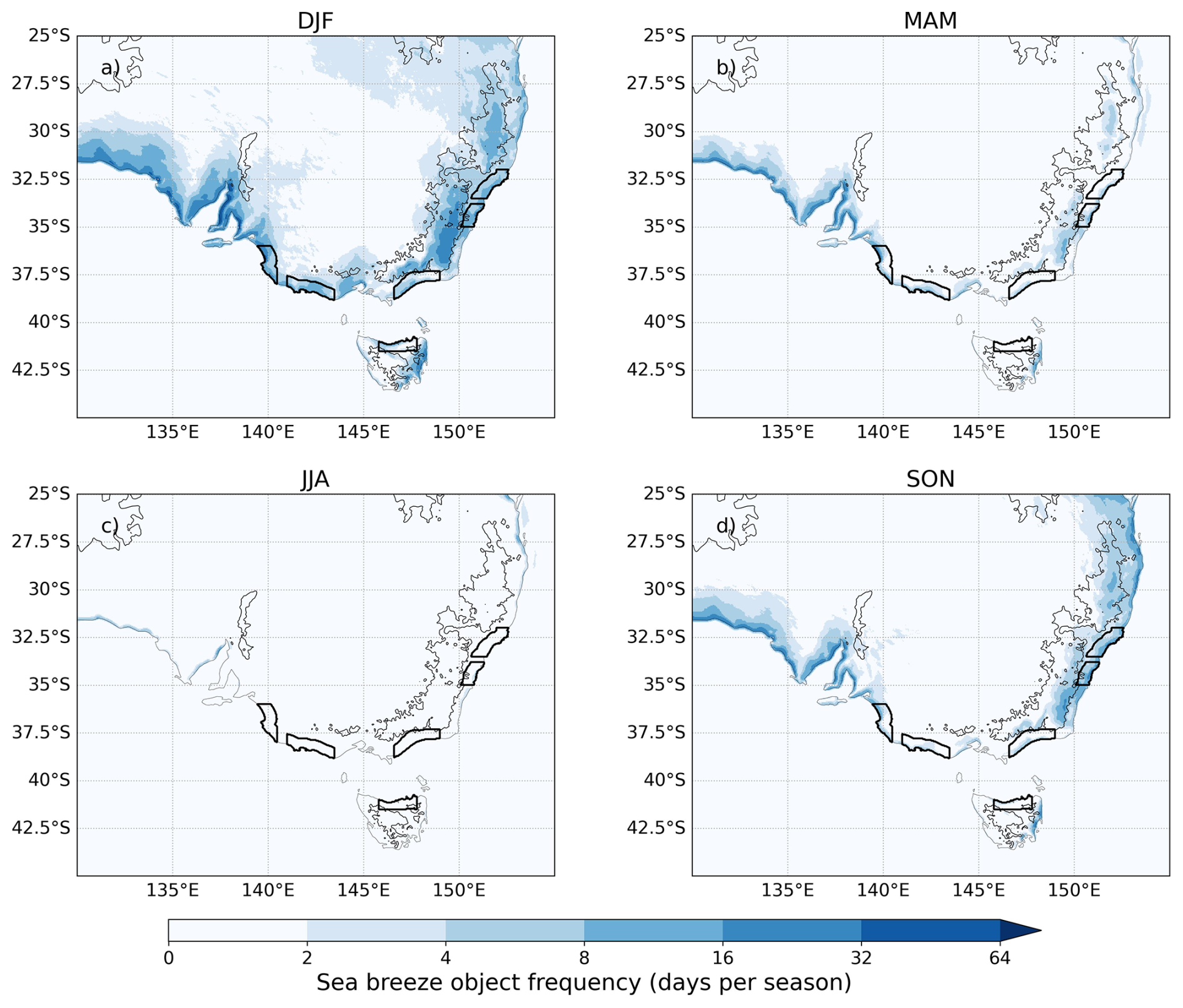
Figure 2 The daily frequency of occurrence of a sea breeze object, shown as days per season for (a) December–February (DJF), (b) March–May (MAM), (c) June–August (JJA) and (d) September–November (SON), shown for southeastern Australia using data from 1979–2024. Coastal areas are indicated with a black contour that are adjacent to six declared offshore wind areas (see Fig. 1). Note the logarithmic colour scale, intended to highlight inland occurrences of sea breezes. Topography over 500 m used in the BARRA-C2 model is contoured.

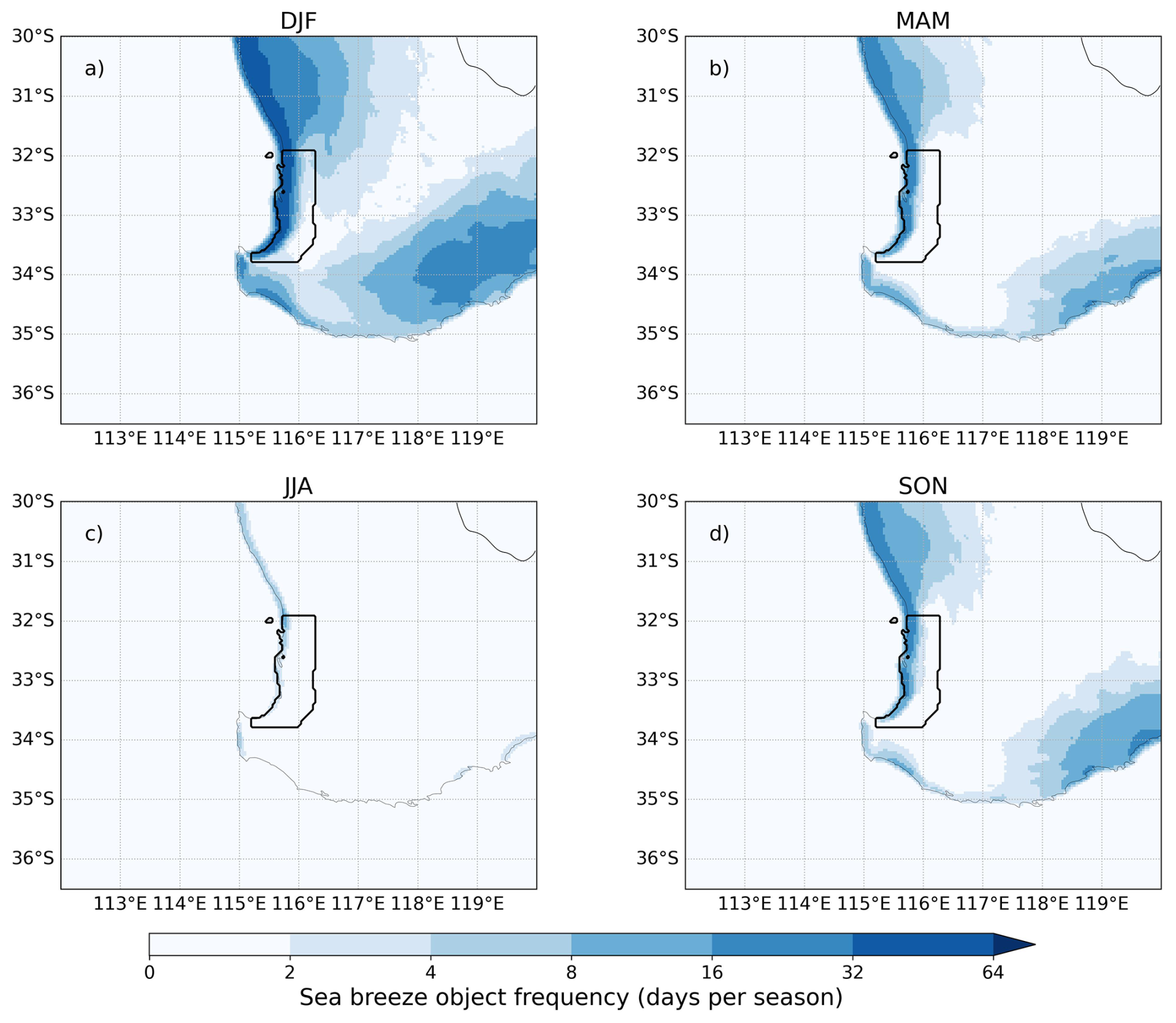
Figure 3 As in Fig. 2 but for southwestern Australia.

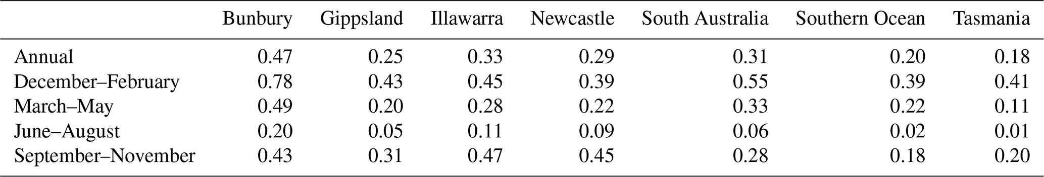
Table 1 Occurrence frequency of days with a sea breeze front (fraction of days) for each coastal land area and season, as well the annual occurrence frequency.

For coastal regions near significant topography, the locations of the local maxima in sea breeze object occurrence frequency tend to be shifted away from the coastline and towards the mountains (Fig. 2). This can be most clearly seen between the coastal land regions adjacent to Gippsland and Illawarra (around 36° S, 149° E). The sea breeze objects identified there are likely produced by a combination of coastal and topographic forcing, which are not able to be easily disentangled. This is consistent with previous idealised modelling studies such as Miao et al. (2003), who have shown that when the sea breeze occurs simultaneously with differential mountain and valley heating, the front between land and sea air occurs further upslope. Inland displacement of detectable sea breeze fronts has also been noted for this region of southeastern Australia by Clarke (1983).

For both southeastern and southwestern Australia, sea breezes tend to occur most often during the austral summer (December–February; Figs. 2a and 3a) when differential land–sea surface temperature gradients are largest. The exception appears to be along the east coast of Australia north of 35° S, where sea breeze objects occur most frequently in the austral spring (September–November; Fig. 2d). The seasonal cycle is examined in more detail in Fig. 4, in terms of sea breeze front (SBF) days for each of the coastal land areas adjacent to the offshore wind areas. For each region, the maximum in SBF days occurs some time during the warm season (October–February), with some variations in the peak month between locations. The maximum monthly SBF day occurrence frequency ranges from around 40 % of days in the Southern Ocean area (February) to 80 % of days in the Bunbury area (January). The minimum occurrence frequency ranges from around 20 % in the Bunbury region to nearly 0 % in several regions during June–August. The occurrence frequency in each coastal area is summarised in Table 1.

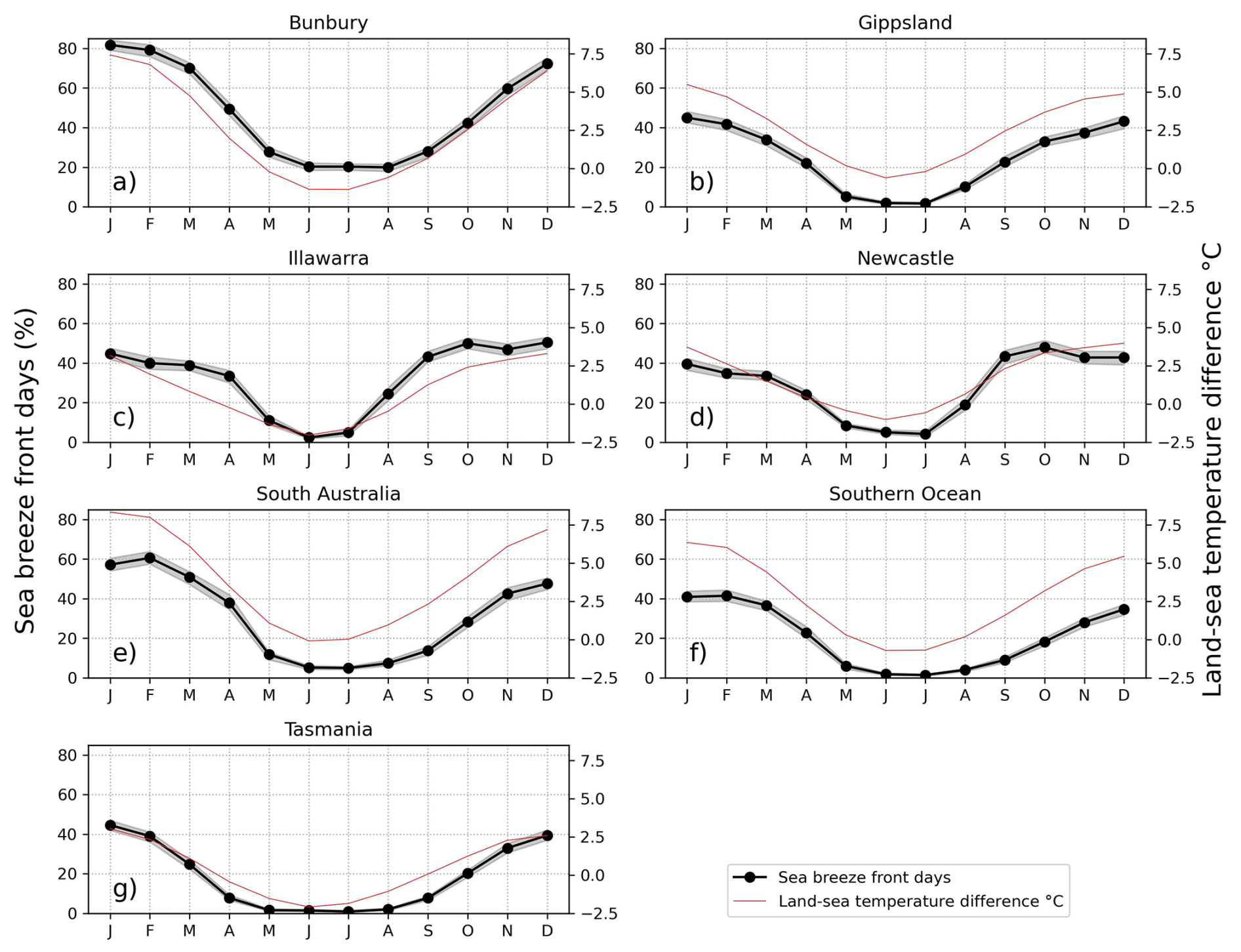
Figure 4 Black line: monthly occurrence frequency of a sea breeze front day for each coastal land area adjacent to the potential offshore wind areas. Shown as a percentage of days. A 90 % confidence interval is indicated with grey shading, estimated by randomly resampling different years of data 1000 times with replacement. The average daily maximum land–sea temperature contrast (°C) is shown for comparison (red lines).

Figure 4 also shows the mean daily maximum T_land−T_sea for each month. The seasonal SBF day cycle generally follows the same shape as the seasonal cycle in mean T_land−T_sea, with a Pearson correlation coefficient of 0.74 over all regions combined. However, for some regions, the peak in SBF day frequency occurs earlier in the year relative to the peak in mean T_land−T_sea. For example, for the Newcastle and Illawarra regions (both on the east coast), SBF day frequency peaks in October (around 50 % of days), even though the monthly mean T_land−T_sea peaks in December–January. This suggests that other factors are influencing the seasonal cycle of SBF days besides the land–sea temperature difference, such as the prevailing wind. Alternatively, the average land or sea temperatures in a broader region may not be an accurate estimate of sea breeze forcing (see Sect. 2.3). In addition, the variations in SBF day occurrence frequency between regions does not appear to be driven only by differences in the magnitude of T_land−T_sea. For example, Illawarra and Gippsland have approximately the same percentage of SBF days in January (just under 50 %), even though the mean T_land−T_sea varies from around 5 °C (for Gippsland) to around 3 °C (for Illawarra).

3.2 Wind resources on sea breeze front days and other days

Figure 5 shows the average diurnal cycle of wind energy capacity factor, averaged over each offshore wind area for SBF days and other days during the summer (December–February). Capacity factors are compared with the average diurnal cycle of regional operational energy demand over the 2010–2019 period. The December–February period is analysed here, given the relatively high occurrence frequency of an SBF day for most regions (Fig. 4), combined with the expectations for hot summertime temperatures leading to increased energy demand (Richardson et al., 2025). Although summer is the focus, results for other seasons are shown in the Supplement (Sect. S3) and are summarised later in this section.

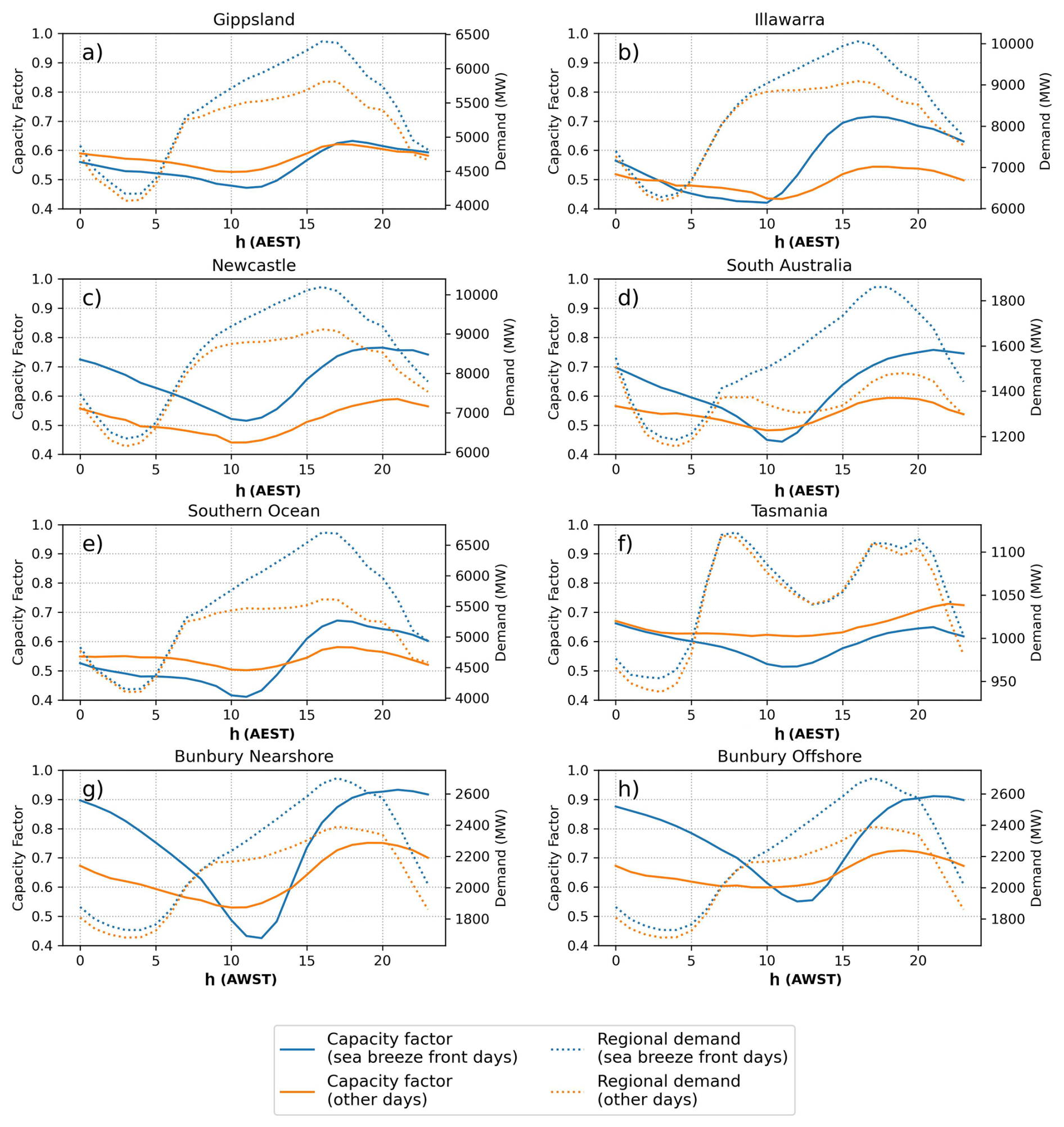
Figure 5 Wind energy capacity factor for each hour of the day during December–February 1979–2024, averaged over each offshore wind area, shown separately for (blue line) sea breeze front days and (orange line) other days. The average regional operational energy demand for each hour of the day, using data from 2010–2019, is shown with dotted lines for comparison. Times shown are Australian Eastern Standard Time (a–f, AEST, UTC+10) and Western Standard Time (g–h, AWST, UTC+8).

For all regions besides Gippsland and Tasmania, the afternoon wind energy potential is around 15 %–30 % higher on SBF days compared with other days, suggesting that the sea breeze has a positive impact on wind energy resources in those regions during the summer. However, sea breezes may also occur on days with weak prevailing winds, with reduced wind energy potential throughout the morning (e.g. the Southern Ocean area, Fig. 5e). In addition, there is typically a lull in wind speeds prior to the formation of the sea breeze at around 10:00–12:00 local standard time. As a result, for all regions besides Newcastle, the wind energy potential is reduced on SBF days at some point in the late morning relative to other days. Together, these results demonstrate that although the sea breeze is a source of local wind and typically enhanced wind energy in the afternoon during the summer, it may not always increase wind energy potential due to its opposition of the existing prevailing wind. For Gippsland and Tasmania, the afternoon wind speed capacity factor is similar, or slightly reduced, on average for SBF days and other days, or slightly reduced on SBF days.

Given the late-morning lull and enhanced afternoon winds on SBF days for most regions, the amplitude of the diurnal cycle in capacity factor is generally much larger on those days compared to other days. For example, in the Bunbury Nearshore area (Fig. 5g), the average capacity factor on SBF days ranges from 0.43 (at 12:00 AWST) to 0.93 (at 21:00 AWST). In contrast, on other days, there is a reduced (but still significant) diurnal variation in capacity factor over that area (from 0.52 at 10:00 AWST to 0.75 at 19:00). These diurnal variations on other days may be due to weak sea breezes that are not detected by the identification methods or other diurnally forced processes such as vertical mixing of winds from aloft to the surface with daytime heating.

For regions with enhanced wind energy potential on SBF days, the late-afternoon or early-evening peak generally coincides with the time of peak operational energy demand (Fig. 5b–e, g, h). This demonstrates the value of wind energy associated with the sea breeze. In addition, Fig. 5 indicates that regional demand is generally higher on SBF days compared with other days. This is likely due to higher surface air temperatures over the land on SBF days (Sect. S4 in the Supplement), consistent with hotter land surfaces for sea breeze forcing, which in turn increases the demand load from cooling. The exception for this relationship is the region of Tasmania, where it has been shown previously that energy demand does not increase with hotter maximum temperatures (Richardson et al., 2025).

In contrast, for other seasons of the year besides summer, the magnitude of the afternoon peak in energy demand is similar between SBF days and other days (see Sect. S3 in the Supplement). This is likely due to cooler temperatures over the land on SBF days compared with SBF days during the summer period, with less electricity demand from cooling. In addition, for the regions identified earlier with enhanced afternoon wind energy potential on SBF days during the summer, this effect is significantly reduced in other seasons (see Sect. S3 in the Supplement). Therefore, some of the potential benefits from sea breezes in supplying wind energy on high-demand days are most relevant during the summer. However, the diurnal cycle in wind energy does still tend to peak at a similar time to peak energy demand during other seasons, with the exception being the austral winter (June–August) when sea breezes are not as common (see Sect. S3 in the Supplement).

Figure 6 shows the average wind direction throughout the day on SBF days and other days during the summer (December–February). The average wind field on SBF days consists of several different types of sea breeze, associated with the direction of the prevailing background winds in the morning. This includes “pure” sea breeze conditions with predominately offshore winds in the morning (Gippsland and South Australia; Figs. 6a, d) and “corkscrew” sea breeze conditions with the land to the right of the prevailing winds (Illawarra, Newcastle, Southern Ocean, Tasmania, Bunbury Nearshore and Offshore; Figs. 6b, c, e–h). In the afternoon, the sea breeze direction may either be mostly on-shore or along-shore. Along-shore flow has been shown by previous studies, including in Brazil (Assireu et al., 2024) and Perth (near the Bunbury area; see Rafiq et al., 2020), due to the interaction of the sea breeze with the synoptic wind direction. Relatively strong along-shore prevailing winds in some regions may potentially relate to the presence of coastal low-level jets. These can be forced by land–sea temperature differences on synoptic scales and have been shown to occur in several places around the globe, including Australia (Ranjha et al., 2013).

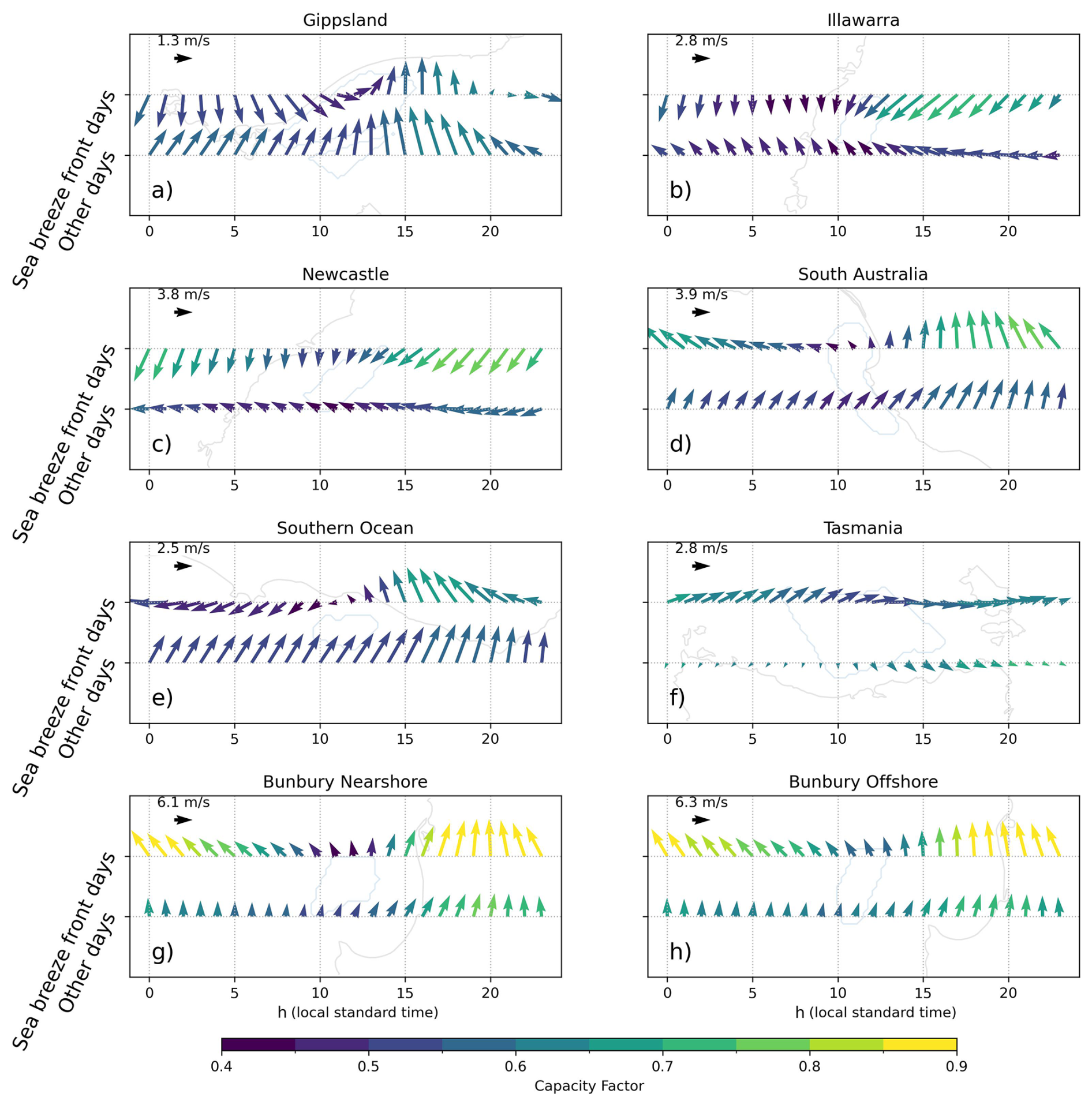
Figure 6 Hourly 100 m u and v wind components averaged over each offshore wind area for each hour of the day during December–February, shown as wind vector plots separately for sea breeze front days (upper vectors) and other days (lower vectors). Vectors are coloured by the corresponding average capacity factor. The coastline and offshore wind areas are shown in the background of each panel for reference in grey and blue contours, respectively.

On summer days without an SBF, the prevailing background wind in the morning may already be onshore (e.g. in the Gippsland region; see Fig. 6a) or be along-shore with the land to the left of the prevailing wind (e.g. in the Illawarra region; see Fig. 6b). In the latter case, the afternoon winds turn onshore and could represent weak backdoor sea breezes with weak frontal gradients. In the former case with onshore prevailing winds, the wind speeds strengthen during the afternoon. This could be due to sea breeze circulations embedded within the onshore flow that may have weak fronts, potentially too weak to be identified (Reible et al., 1993). Alternatively, the afternoon strengthening of winds could be related to other mechanisms such as the vertical mixing of higher wind speeds to near the surface with daytime heating. However, the potential for weak sea breezes to exist on “other days” should be noted when interpreting results. In summary, sea breezes are interpreted here as coastal circulations leading to strong fronts over the land, with weaker circulations possible on other (non-SBF) days. The results in this section suggest that stronger circulations with fronts over the land are more relevant for wind energy resources (Fig. 5).

The relationship between prevailing wind direction and December–February SBF frequency, as well as afternoon wind energy capacity factor, is quantified further in the Supplement (Sect. S5). This is done by separating SBF days into four prevailing wind quadrants, depending on if the wind is onshore or offshore with land to the right or left. Those results support the findings here that offshore winds are generally favourable for SBF days, while there are significant variations in afternoon capacity factor based on the prevailing wind direction.

3.3 Co-variability of sea breeze front days across wind energy zones

In Sect. 3.2, it was demonstrated that sea breeze front (SBF) days and other days have different prevailing winds in the morning (Fig. 6), suggesting that the background wind direction has a strong influence on sea breeze formation, consistent with previous studies (Arritt, 1993; Steele et al., 2013). It follows that for a given large-scale wind pattern over southeastern or southwestern Australia, there will be coastal regions where sea breeze fronts are more or less likely to be identified due to prevailing winds being onshore or offshore in different regions, for example. This is demonstrated here for two offshore wind areas with opposite-facing coastlines during the December–February period: Illawarra and Southern Ocean (see locations in Fig. 1b).

Figure 7a shows that in the early morning (05:00 AEST) on Illawarra SBF days, there is a synoptic pattern with northerly along-shore winds relative to the Illawarra coastline, on average. As discussed in Sect. 3.2, this is favourable for corkscrew sea breeze formation. At the same time, this synoptic pattern produces onshore prevailing winds for the Southern Ocean area that generally favours non-SBF conditions (Fig. 7a). In the afternoon, strong onshore flow develops in the Illawarra region (Fig. 7c), whereas in the Southern Ocean region, the onshore winds have only increased in magnitude (consistent with the wind direction on other days for the Southern Ocean region in Fig. 6e). This suggests sea breeze front formation in the Illawarra region, while for the Southern Ocean region, the afternoon winds may have strengthened due to weak coastal circulations embedded within the prevailing flow or due to the vertical mixing of higher wind speeds from aloft.

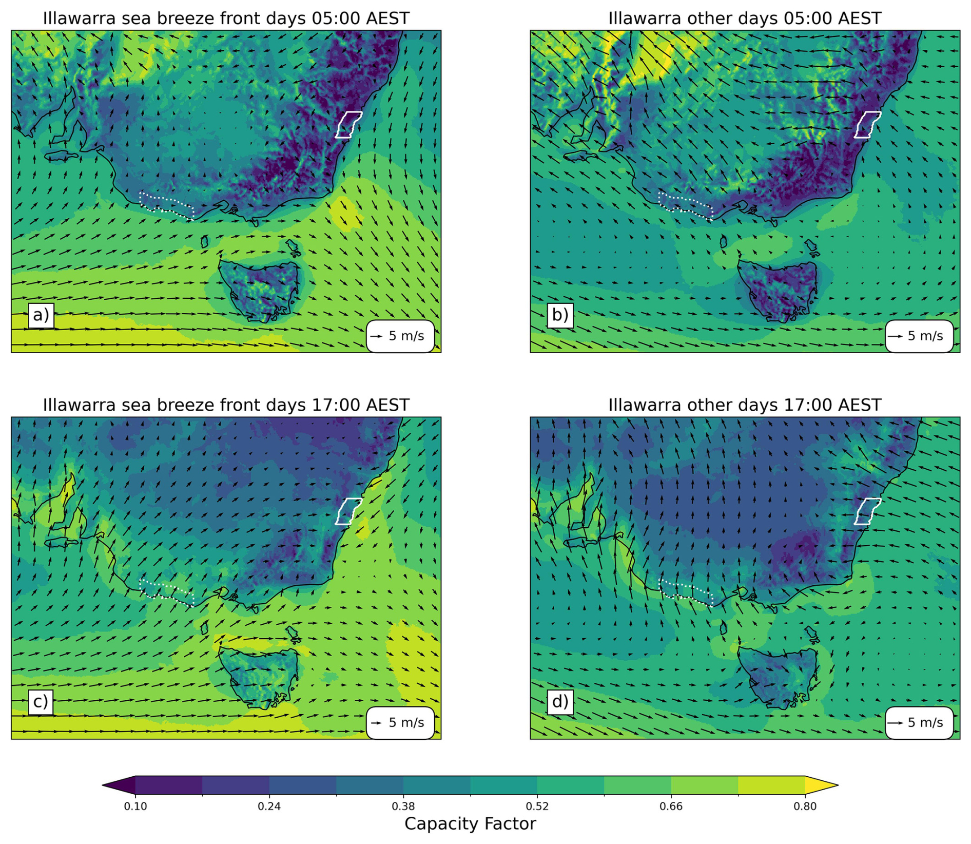
Figure 7 Spatial map of 100 m u and v wind components and capacity factor, averaged over (a, c) sea breeze front days and (b, d) other days for the Illawarra offshore wind area. Legends demonstrating the length scale of the wind vectors are shown in the bottom right of each panel. Averages are calculated during December–February for (a, b) 05:00 Australian Eastern Standard Time (AEST) and (c, d) 17:00 AEST. The location of onshore coastal areas adjacent to the Illawarra and Southern Ocean offshore wind areas are highlighted with a solid and dotted white contour line, respectively.

Conversely, on days without an SBF in the Illawarra region, there is onshore flow there in the morning (Fig. 7b), with along-shore flow relative to the Southern Ocean coastline with land to the right, favourable for corkscrew sea breeze formation. In the afternoon, the opposite pattern can be seen compared with SBF days in the Illawarra region: strong onshore flow has developed in the Southern Ocean region, whereas in the Illawarra region, the onshore winds have only increased in magnitude (Fig. 7d). For completeness, Fig. 8 shows the same analysis but for Southern Ocean SBF days and other days. The figure essentially demonstrates the inverse pattern, whereby the Southern Ocean SBF days occur with offshore flow in the morning, with unfavourable SBF conditions for the opposite-facing Illawarra coastline.

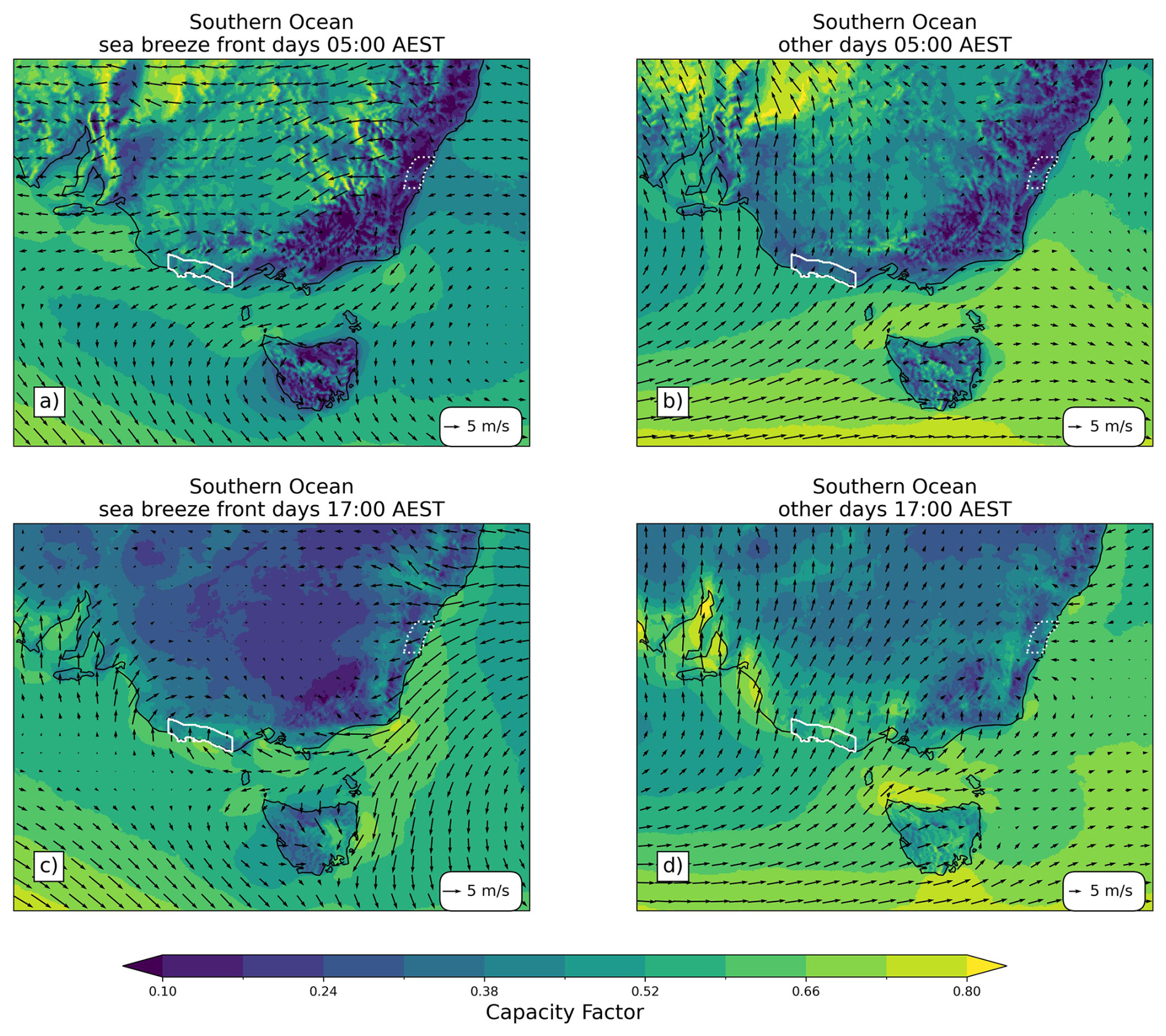
Figure 8 As in Fig. 7 but on sea breeze front days and other days for the Southern Ocean offshore wind area. The location of onshore coastal areas adjacent to the Southern Ocean and Illawarra offshore wind areas are highlighted with a solid and dotted white contour line, respectively.

Figure 9 extends this analysis, showing anomaly maps of sea breeze objects identified on SBF days for each offshore wind area during December–February. This figure demonstrates that when sea breezes are identified on east-facing coastlines (Illawarra, Newcastle or Gippsland), they are less likely to be identified on west-facing coastlines (including South Australia or Southern Ocean) due to the orientation of the prevailing winds, similar to the example shown previously for the Illawarra and Southern Ocean regions. The opposite is true when sea breeze fronts are identified on the west-facing coastlines (that is, negative anomalies are seen over the east-facing coastlines on those days), and the same effect can be seen for north- or south-facing coastlines (Tasmania and Southern Ocean; Fig. 9f) and the adjacent coastlines in southwestern Australia (Fig. 9g). The correlation of SBF day occurrences between each region in southeast Australia is quantified further in the Supplement using the odds ratio (Sect. S6). That analysis shows, for example, that the odds of an SBF day occurring in the Illawarra or Southern Ocean regions is approximately halved when an SBF day occurs in the other region. In contrast, the odds of an SBF day occurring in Illawarra or Gippsland is 2.7 times higher when there is an SBF day in the other region.

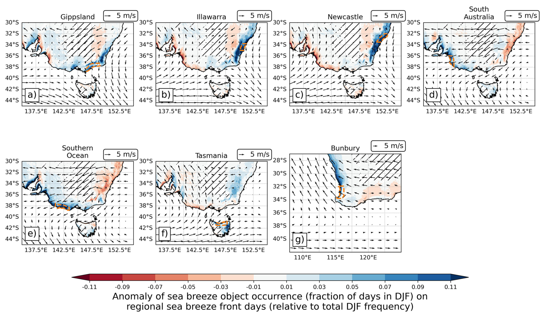
Figure 9 Map of sea breeze occurrence anomaly (fraction of days with the occurrence of a sea breeze object) between regional sea breeze front (SBF) days and total days for December–February. Positive values for a given region represent a greater frequency of sea breeze object occurrences, compared with the frequency on all days. In each panel, the average u and v wind components over all SBF days for that region at 05:00 local standard time are shown with vectors, as an estimate of the prevailing background wind. Legends demonstrating the length scale of the vectors are shown above each panel. The coastal area that is used to define regional SBF days is highlighted with an orange contour line. Hatching represents areas with a total daily sea breeze occurrence frequency of less than 1.5 % (equivalent to 1.35 d per December–February period; see maps in Figs. 2a and 3a), where data have been removed from the plot for clarity.

Finally, this behaviour is related to late-afternoon available wind energy (18:00 local standard time) by showing spatial maps of the difference in capacity factor between regional SBF days and other days (Fig. 10). The 18:00 local standard time difference is approximately the time of peak energy demand and sea breeze wind speeds (Fig. 5). For the regions of Illawarra, Newcastle and Gippsland, there is generally more local available offshore wind energy on SBF days along the east coast (up to a 0.1–0.2 increase in capacity factor; Fig. 10a–c). There is similar or reduced available offshore wind energy along the South Australia and Southern Ocean regions (up to a 0.1 reduction), likely due to a reduction in sea breeze activity as described previously (Fig. 9). In addition, there are localised reductions in available wind energy in the inland regions adjacent to each of the coastal regions where SBFs are identified (by as much as 0.2–0.3 in capacity factor) but with a general increase in available wind energy across large parts of inland southern Australia, likely due to enhanced synoptic-scale wind speeds.

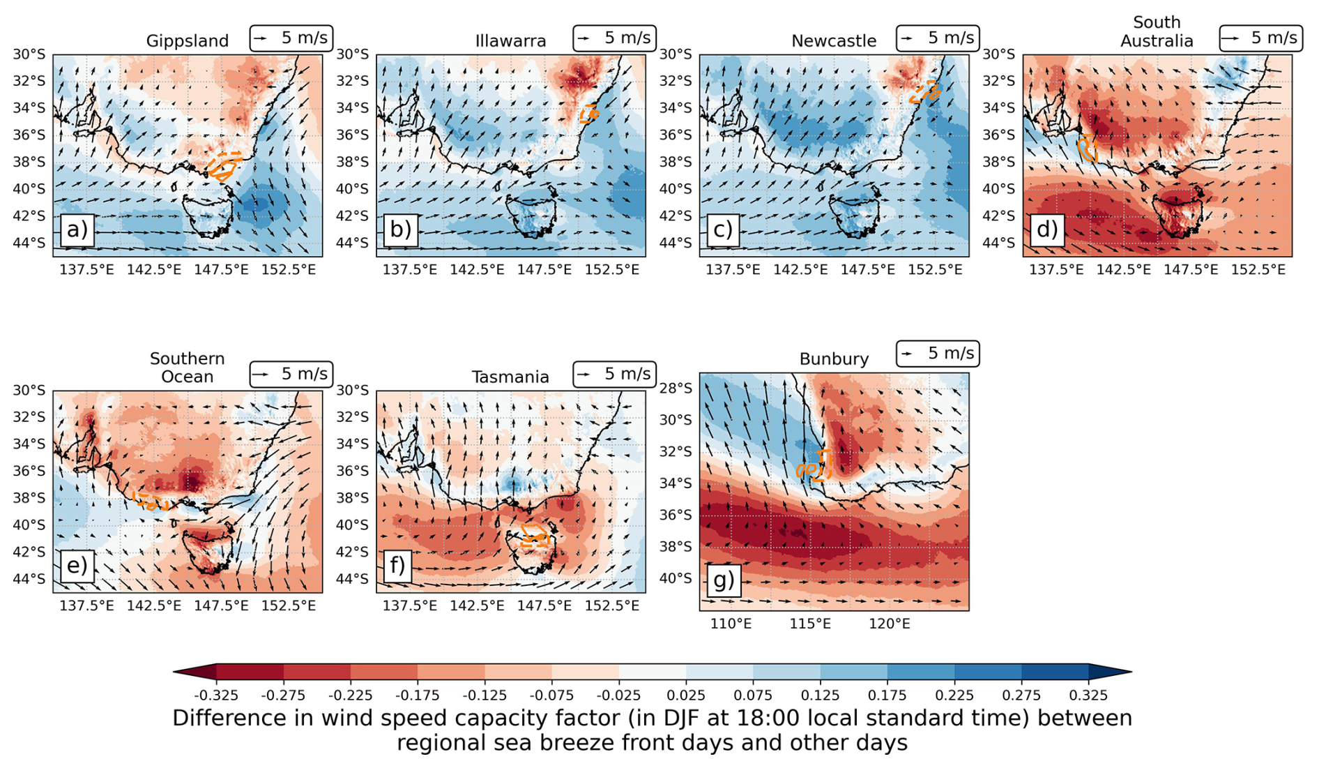
Figure 10 Map of the difference in wind energy capacity factor between regional sea breeze front (SBF) days and other days at 18:00 local standard time during December–February. Positive values represent higher capacity factors on SBF days compared with other days. Each panel shows the difference in capacity factor for a different region, with the region used to define SBF days shown in the dashed orange contour. The location of the adjacent offshore wind areas are also shown in orange contours. Average 100 m wind vectors on SBF days are shown at 18:00 local standard time. Legends demonstrating the length scale of the vectors are shown above each panel.

In contrast, on SBF days over the west-facing coastal locations of South Australia and the Southern Ocean, there are decreases in local offshore wind energy availability over large sections of the east coast (up to around 0.1 in capacity factor), as well as along the northern coast of Tasmania (Fig. 10d–e), with local increases in available wind energy for the offshore regions of South Australia and the Southern Ocean. Again, this is likely due to the behaviour of sea breeze activity described previously in this section. There tends to be widespread decreases in available wind energy throughout inland parts of southern Australia on these SBF days, potentially due to reductions in onshore synoptic-scale wind speeds. For SBF days in Tasmania (Fig. 10f), there are small local offshore increases in available wind energy due to sea breeze activity but large decreases in offshore regions to the south of mainland Australia (up to a 0.2 reduction in capacity factor). This is likely associated with reductions in synoptic wind speeds, with decreases also in the Gippsland offshore region potentially due to reduced sea breeze activity. On Bunbury SBF days (Fig. 10g), there are significant increases in local offshore wind availability near the Bunbury region and significant decreases inland, as well as offshore to the south of the continent.

4 Discussion

A new method for identifying sea breezes as frontal objects (Brown et al., 2026) has been applied to a km-scale atmospheric reanalysis dataset over Australia for the period 1979–2024. This method has enabled an assessment of sea breeze occurrences for the first time across multiple coastlines in this region, using a single, physics-based diagnostic approach. The spatial and seasonal distribution of sea breeze occurrences are analysed over southeastern and southwestern Australia, with a focus on key potential offshore wind areas.

Maps of sea breeze object occurrence frequency indicate that sea breeze objects are most often identified over coastal land regions during the austral summer and spring (September–February), with some variations between regions (Figs. 2–4). For example, in southern regions such as Gippsland, the peak in the proportion of days with a sea breeze object is in December–January (45 % of days; see Fig. 4b), whereas for more northern regions such as Newcastle, the peak is in October (50 % of days; see Fig. 4d). This latter maximum during the austral spring is similar to findings for the relatively northern region of southeast Queensland by Soderholm et al. (2017), while the maximum in summer for the southern regions is similar to other studies near the Bunbury and South Australia regions (Masselink and Pattiaratchi, 2001; Pazandeh Masouleh et al., 2016). Details on the seasonal cycle in sea breeze occurrences for these previous studies can be found in the Supplement (Sect. S2).

The seasonal cycle of sea breeze occurrences broadly appears to follow the monthly mean daily maximum land–sea temperature difference (T_land−T_sea), with a monthly correlation coefficient of 0.74 over all regions. The mean T_land−T_sea is representative of sea breeze forcing and peaks during the warm season due to daytime heating over the land. However, T_land−T_sea cannot explain some details of the seasonal cycle and variations between regions. For example, as discussed previously, Newcastle sea breeze occurrences peak in October, whereas T_land−T_sea is maximised in December–January (Fig. 4d). Although other factors such as the prevailing wind direction may influence the variability in sea breeze occurrences (Arritt, 1993), it is also possible that T_land−T_sea, as defined here, is not an accurate measure of sea breeze forcing. As discussed in Sect. 2.3, there does not appear to be consensus among previous studies on how to define T_land−T_sea. Future work could investigate the spatial and temporal scales of land and ocean temperatures that are relevant for forcing the sea breeze.

During the austral summer (December–February), sea breezes generally provide enhanced wind energy potential in the offshore wind areas examined during the afternoon on average, relative to other days without sea breeze fronts identified. This was observed for six out of the eight offshore wind areas in southeastern and southwestern Australia (all regions except Gippsland and Tasmania; see Fig. 5), although this behaviour is reduced for other seasons in the year (see Sect. S3 in the Supplement). In contrast, for all but one of the offshore wind regions (Newcastle), sea breeze formation was associated with decreased wind energy potential during the morning on average. This could be due to preferential sea breeze formation on days with relatively weak prevailing winds, as well as sea breeze surface winds that oppose the existing prevailing winds. The latter process is consistent with a late-morning minimum in capacity factor for most regions, at around 10:00 to 12:00 local standard time, prior to the onset of the sea breeze (Fig. 5). These calm periods prior to sea breeze formation have been previously described as offshore “calm zones” by previous studies (Steele et al., 2015) and have implications for the diurnal cycle of wind energy capacity factor in coastal regions.

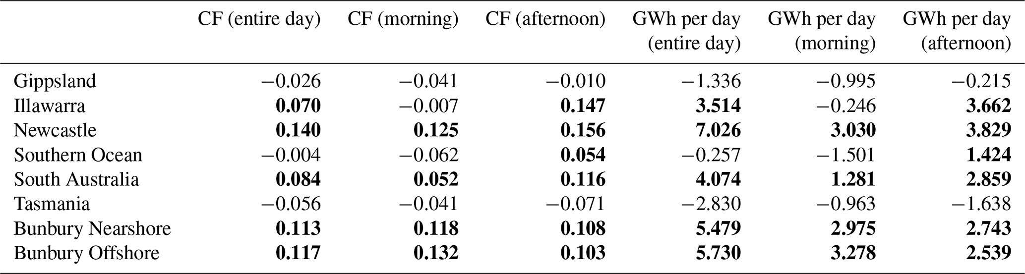
The difference in wind resources between sea breeze front days and other days during the summer is summarised in Table 2, for each offshore wind area. This is quantified based on the difference in average daily profiles of capacity factor shown in Fig. 5. This is intended to provide an approximate quantification of the wind energy surplus or deficit associated with sea breeze conditions, including the sea breeze itself in addition to the prevailing winds. In addition, Table 2 also reports the difference in integrated energy output calculated from these average daily profiles of capacity factors, based on a theoretical wind farm with a capacity of 2.2 GW (ignoring any energy losses). This represents the planned capacity of a wind farm currently in development in the Gippsland offshore wind area. An equivalent table using capacity factor differences from annual data is shown in the Supplement (Sect. S3).

Table 2 Difference in average daily capacity factor (CF) and theoretical wind energy generation (in GWh per day) between days with a sea breeze front and other days during December–February. Positive values (in bold) represent surplus CF or GWh on sea breeze front days. Calculated separately using all daily data, as well as for the morning only (00:00–11:59 local standard time) and afternoon/evening (12:00–23:59 local standard time). Theoretical wind energy generation is based on a 2.2 GW capacity wind farm.

Sea breezes are shown to typically be identified on days during summer with relatively high regional operational energy demand on average (Fig. 5). This is likely due to the tendency for sea breezes to occur on days with hot surface air temperatures over the land (see Sect. S4 in the Supplement), providing an enhanced land–sea thermal contrast for sea breeze forcing, while also increasing electricity demand for the cooling of residential buildings, although this is not observed during other seasons (see Sect. S3 in the Supplement). Furthermore, wind energy capacity factors on days with a sea breeze identified tend to peak at a similar time to energy demand, meaning that offshore wind could potentially provide a useful source of energy during peak demand periods. This is similar to the findings of Pickering et al. (2020) in the alpine regions of Switzerland, who found that diurnal variability in wind resources tends to peak in the afternoon during the summer, due to topographically forced local winds. Afternoon peaks in local wind energy resources, including due to the sea breeze, could also offset the diurnal reduction in solar energy production in the late afternoon.

The results in Sect. 3.2 demonstrate that days with a sea breeze identified and days without a sea breeze have a very different prevailing wind direction in the morning for a given region, on average (Fig. 6). This is consistent with many previous studies that have shown the prevailing wind to have a strong impact on the occurrence of sea breezes and/or detectable fronts (e.g. Arritt, 1993; Reible et al., 1993), and therefore the diurnal cycle of wind energy potential (Steele et al., 2015). For example, onshore winds in the morning were found to occur on days without a sea breeze front, as evidenced by the morning wind direction (e.g. in Gippsland; Fig. 6a). As a result, for a given synoptic-scale wind (westerlies, for example), there are some coastlines with favourable sea breeze conditions, including offshore prevailing winds (east facing for westerly prevailing winds) and some with unfavourable conditions including onshore prevailing winds (west facing for westerly prevailing winds). This can be seen in the sea breeze object dataset, with sea breeze occurrences tending to cluster on east- and west-facing coastlines (Fig. 9). This is consistent with previous studies that have investigated sea breeze characteristics for sets of idealised opposing coastlines (Steele et al., 2013) but is shown here for all coastlines throughout a regional domain using a dataset of sea breeze objects. The clustering of sea breezes on east- and west-facing coastlines can also affect the late-afternoon wind energy availability in different regions (Fig. 10) and may therefore have implications for managing afternoon energy demand and supply, assuming that these regions of energy generation could be connected in the same system. Results here suggest that diversifying wind generation to multiple coastlines could provide added energy security on high-demand days, particularly during the critical late-afternoon high-demand period.

The findings here are based on the separation of days with a sea breeze and days without a sea breeze. This separation is defined using the occurrence of a moisture front over the land associated with the sea breeze circulation. However, there are uncertainties in defining these sets of days. For example, coastal circulations are possible (in theory) whenever there is a gradient in surface temperature along the coastline, but here we only define a sea breeze when there is a front that exceeds a certain threshold (see Sect. 2.1). Figure 6 suggests that there is some turning and strengthening of the wind on days without an identifiable sea breeze front (e.g. in the Illawarra region; Fig. 6b). This could represent weak coastal circulations without the formation of a strong sea breeze front, and some of the average “other day” wind profiles in Fig. 6 could be classified as backdoor sea breeze conditions following other studies (Miller et al., 2003). There is also potential evidence for circulations embedded in onshore prevailing winds that may not have strong frontal gradients (Reible et al., 1993), based on afternoon increases in onshore winds on some “other day” profiles (Fig. 6). In addition, the diurnal variability of the winds on days with a sea breeze object could be produced by several different mechanisms. Aside from the sea breeze, this could also include topographically forced circulations (upslope mountain breezes), outflow from convection or the vertical mixing of winds from aloft to the surface, for example. The disentangling of these different processes is important for considering the relative contributions of different local wind processes to energy resources and could be the focus of additional modelling work in the future.

Finally, the results presented here are subject to uncertainties in the representation of sea breezes and associated capacity factors using a reanalysis model dataset (BARRA-C2) and 10 MW wind turbine power curve (Sect. 2.4). Similar reanalysis models have been shown previously to have significant errors at certain times of the day (Davidson and Millstein, 2022), and, therefore, further evaluation of these reanalysis datasets using wind data at hub height is a critical avenue of future work for wind resource research. The choice of a 10 MW power curve here was intended to represent a turbine of a realistic size, but it is acknowledged that different turbines may be more suitable for the different regions analysed here, due to potential variations in mean wind speeds. This could potentially bias the capacity factors reported here for certain regions. In addition, we have used a power curve for a single wind turbine to represent wind energy resources, when in reality this may be reduced by wake effects in a wind farm. These wake effects would likely be sensitive to wind direction, which is influenced by the sea breeze. The influence of the sea breeze on wind farm wake effects could be another potential avenue for future work.

5 Conclusion

We investigated the impact of sea breezes on offshore wind resources in southeastern and southwestern Australia, using a historical dataset of sea breeze objects during the period 1979–2024. The key findings are listed as follows:

• Sea breeze occurrences in southeastern and southwestern Australia generally follow a similar seasonal pattern to the mean daily maximum land–sea temperature contrast, with both generally peaking during the austral summer. However, some regions (northeastern coastal regions including Newcastle and Illawarra) have a peak in sea breeze occurrences shifted to the austral spring (September–November), earlier than the maximum in land–sea temperature contrast.

• For six out of the eight offshore wind areas examined here, there is around 15 %–30 % more available wind resources on sea breeze front days during the afternoon in the austral summer compared with other days. In contrast, there are generally fewer available wind resources during the morning on sea breeze front days due to calm periods where the sea breeze flow opposes the existing prevailing wind.

• Sea breezes during the summer are generally shown to occur on days with high regional energy demand, with an afternoon peak in wind energy that broadly aligns with the afternoon peak in demand. Therefore, wind energy associated with the sea breeze is potentially valuable for balancing energy demand during afternoon peak periods in the summer.

• When sea breezes occur on east-facing coastlines, they are less likely to occur on west-facing coastlines (and vice versa) due to the role of the prevailing winds in providing favourable conditions for formation. This has implications for the correlation of afternoon wind resources between regions.

These results could help to guide strategic decisions on offshore wind farm development and energy system planning, with the goal of providing reliable energy supply in the Australian network. For example, results here suggest that offshore wind energy placed along a range of diverse coastal areas could help with balancing demand in the Australian energy market during the afternoon, especially on hot, high-demand days. More broadly, we have highlighted the importance of sub-daily local wind variations (in this case, the sea breeze along the coast) for providing wind energy resources and therefore the need for sufficiently high-resolution data to capture these variations in resource assessments (such as a km-scale reanalysis, as in this case). In addition to sea breezes, local wind variations can be associated with topographic flows or low-level nocturnal jets, for example. These local wind variations should be considered when assessing potential wind farm sites or the performance of energy systems with large amounts of wind energy. Future work should continue to assess the impact of local wind processes, including sea breezes, on wind energy resources, both onshore and offshore.