Wind speed estimation using second-order sliding-mode observers: simulation and experimental validation on a floating offshore wind turbine

Rotor-effective wind speed (REWS) estimation is crucial for the control and performance optimization of floating offshore wind turbines (FOWTs). This paper introduces a robust estimation framework based on second-order sliding-mode observers (SOSMOs), developed in both constant-gain and adaptive versions. The observers are developed using a reduced-order dynamic model and validated in the OpenFAST simulation environment when all degrees of freedom are activated. Their performances are compared with the continuous–discrete extended Kalman filter (CD–EKF) used in the reference open-source controller (ROSCO). The proposed approach is assessed under stochastic wind/wave conditions through OpenFAST simulations and further validated experimentally using a scaled software-in-the-loop (SIL) setup. Simulation results indicate that the proposed observers perform comparably to the CD–EKF in terms of estimation accuracy while offering robustness, simpler implementation, and reduced computational complexity.

1 Introduction

The increasing global demand for electricity has necessitated the exploration of sustainable energy solutions, with offshore wind energy emerging as a key contributor. As the scale and penetration of wind energy continue to grow, the technology is pushed into new scientific and engineering challenges related to atmospheric flow uncertainty, turbine dynamics, and wind plant control and integration (Veers et al., 2019). Floating offshore wind turbines (FOWTs) offer access to vast, underutilized wind resources located in deep waters, which account for approximately 80 % of the global offshore wind potential, as reported by Global Wind Energy Council (2022). Compared with fixed-bottom turbines, FOWTs benefit from stronger and more consistent winds; however, the floating structure introduces additional degrees of freedom, such as platform motions, which can cause negative damping and exacerbate power fluctuations. In extreme cases, this instability could lead to system failure. Consequently, conventional strategies developed for onshore wind turbines are not sufficiently effective for floating ones. Therefore, advanced estimation and monitoring approaches are required to support the stability and efficiency of FOWTs (McCoy et al., 2024; Stockhouse et al., 2024).

The operation of wind turbines is typically divided into four regions based on the prevailing wind speed (Stockhouse et al., 2024). In Region I (below the cut-in wind speed), the turbine sits idle waiting for the wind speed to increase, as the available wind energy is insufficient to operate the turbine. In Region IV (above the cut-out wind speed), the turbine also stops operating to prevent potential damage. In contrast, power generation occurs in Region II and Region III, each employing distinct control strategies. In Region II, the objective is to maximize the power coefficient to optimize energy capture, whereas in Region III, the objective is to keep the power at its nominal value. Indeed, maintaining power at its rated level is essential to protect the turbine and ensure its longevity and operational stability.

In the operation of FOWTs, accurate information about wind speed is a fundamental requirement for control system design, real-time monitoring, and ensuring the safe and efficient performance of the turbine (Soltani et al., 2013). Wind speed information serves multiple critical functions depending on the control strategy employed. For example, in Region II, wind speed is used to compute the optimal rotor speed reference based on the desired tip-speed ratio, whereas in Region III, it plays a central role in blade pitch control action (Stockhouse et al., 2024). Furthermore, wind speed measurements are a key input for feed-forward control algorithms. The quality of wind speed information thus has a direct impact on the overall performance and longevity of FOWTs.

Different methods exist in the literature regarding wind speed measurement or estimation on FOWTs, including sensor-based, observer-based, and neural-network-based approaches.

• Lidar use. An advanced remote-sensor-based method commonly used is light detection and ranging (lidar), which can sample the wind field upstream of the turbine to provide a measurement of upstream wind speed (Harris et al., 2006; Shu et al., 2016). A considerable amount of literature has demonstrated the potential of lidar-assisted control for performance improvement and load mitigation in wind turbines, such as He et al. (2025), Moldenhauer and Schmid (2025), Li and Geng (2024), Guo and Schlipf (2023), Mahdizadeh et al. (2021), Schlipf et al. (2023), and Guo et al. (2023). Simley et al. (2020) provide an overview of recent advances and open problems in the use of lidar for enhancing wind turbine operation and control. Despite the significant progress achieved in this area, some practical limitations remain. One of the most apparent limitations is the cost and the maintenance demand of these systems (Jena and Rajendran, 2015; Woolcock et al., 2023). Lidar devices, particularly those used in offshore and floating structures, are expensive to acquire and install, and their operation in harsh marine environments imposes high standards on longevity, autonomous operation, and regular maintenance to guarantee data quality. In addition, a primary technical limitation lies in the vulnerability of lidar measurements to motion-induced errors. Floating platform motions distort the lidar’s line of sight and also the apparent wind speed because of the lidar translation, introducing systematic biases and increased uncertainty in wind speed estimation (Gräfe et al., 2023). Such disturbances can lead to errors in real-time control. Moreover, lidar measurements inherently suffer from limited correlation with the actual wind field impacting the rotor, since wind is measured several rotor diameters upstream and evolves due to turbulence, while volume averaging and point-wise sampling prevent reconstruction of the exact rotor-scale wind field, introducing unavoidable uncertainty in the measured REWS (Svenstrup and Thomsen, 2024). These limitations highlight the need for alternative or enhanced wind speed estimation techniques that are accurate, sensorless, and therefore more cost-effective.

• Neural-network-based methods. Alternatively, some recent studies rely on neural-network-based methods for wind speed estimation and forecasting (Zhang et al., 2024; Sierra-García and Santos, 2021; Pan et al., 2022). These methods typically require an offline training phase using large datasets that must accurately represent the system’s operating conditions (Chen and Han, 2022). However, deep learning models behave like black boxes, offering limited interpretability and making it difficult to guarantee and formally prove stability or robustness of the closed-loop system. Additionally, the generalization of these models to unseen conditions remains a significant challenge.

  Another research direction focuses on observer-based wind speed estimation methods, such as the Kalman filter family and immersion and invariance (I&I) estimators. In this context, the present work investigates robust nonlinear observer designs based on sliding-mode theory, after briefly reviewing the main observer-based approaches relevant to this study.

• Kalman filter solution. Another widely adopted alternative is the Kalman filter (KF) and its variants. In Soltani et al. (2013), both linear and nonlinear KFs are used for REWS estimation. The simulation results also showed that the performance of the nonlinear KF is better than the other at the transient state for the reason that the time response of the nonlinear KF is much smaller than that of the linear KF. KFs provide model-based state estimation by integrating a system’s dynamic equations with available sensor measurements. In wind turbine applications, they have been employed to estimate REWS by combining turbine output data with linear aerodynamic models (Boukhezzar and Siguerdidjane, 2011). However, since wind turbine systems are inherently nonlinear, standard KFs do not perform well in dynamic operating conditions. To address this, extended Kalman filters (EKFs) have been developed to handle nonlinearities more effectively. A REWS estimation method based on EKF was introduced in Song et al. (2017) to improve the efficiency of wind turbine operation. By integrating this algorithm with optimal tip-speed ratio tracking, the study demonstrated enhanced control of maximum power output. This paper reported that the proposed method could raise annual energy output by around 0.8 %. In Hernández et al. (2014), the application of an EKF for REWS estimation was demonstrated using real experimental data. This study is particularly noteworthy, as it validates the reliability of the EKF-based estimation method with real-world operating data.

  Furthermore, some studies, such as Chen et al. (2025) and Knudsen et al. (2011), use an indirect method for REWS estimation. In these approaches, aerodynamic torque is first estimated, thus allowing the estimation of REWS. In Kim et al. (2024), two methods of REWS estimation are used and compared. The first one is based on the drive-train model using measured rotor speed, pitch angle, and generator torque as inputs, and the second one involves applying the estimated wind speed using a 3D look-up table and is compared with a continuous–discrete extended Kalman filter (CD–EKF).

  Despite their widespread use, EKF-based methods for estimating REWS have several limitations that restrict their applicability in FOWTs. One key challenge lies in the tuning of process and measurement noise covariance matrices, which is often heuristic and lacks a systematic procedure. Improper tuning can lead to divergence (Chen et al., 2025; Song et al., 2017). Additionally, EKFs require approximation of the model around operating points, making them sensitive to variations in system dynamics and reducing their accuracy in highly nonlinear or time-varying conditions. This is particularly problematic in FOWTs, where platform motions introduce significant nonlinearity. Furthermore, the EKF also suffers from poor robustness to model mismatch and unmodeled dynamics, which are common in offshore environments. Finally, the formal proof of stability of the closed-loop including KF/EKF solutions is not trivial. These drawbacks highlight the need for more robust, model-insensitive alternatives for REWS estimation.

• Immersion and invariance (I&I) estimators. Another class of observer-based wind speed estimation methods is based on immersion and invariance (I&I) theory. I&I estimators exploit invariance principles to construct observers with guaranteed convergence properties (Ortega et al., 2013; Soltani et al., 2013). In Brandetti et al. (2022), a wind speed estimator embedded in a tip-speed ratio tracking control scheme was analyzed using a simplified, linearized aerodynamic model. The authors showed that this scheme is inherently ill-conditioned, in the sense that uncertainty in the power coefficient directly leads to biased wind speed estimates through the power balance equation. In particular, even small variations in power coefficient were shown to cause a systematic bias in the estimated effective wind speed. Unlike that work, the present study relies on a nonlinear aerodynamic model and is validated using the high-fidelity OpenFAST simulator, where the power coefficient inherently differs from its true physical value due to modeling approximations. As a result, the use of robust estimation approaches becomes necessary to mitigate the practical impact of such model uncertainties on wind speed estimation accuracy.

• Observer approach based on sliding-mode theory. Among observer-based approaches, sliding-mode observers (SMOs) have attracted significant attention due to their inherent robustness to uncertainties and disturbances, which are particularly prevalent in offshore environments. The idea of SMOs is to drive the estimated states to properly chosen constraints (the sliding manifold) in finite time and then maintain the sliding mode for all subsequent times so that the state estimation errors are driven to zero, thus exploiting the main features of the sliding mode: its insensitivity to external and internal disturbances matched to the control and its finite time reaching transient. Unlike KFs, which rely heavily on accurate statistical models and noise characteristics, SMOs exploit the system's nonlinear structure and discontinuous logic to force estimation errors to converge in finite time (Ma et al., 2024). This makes them well-suited for FOWTs, where system dynamics are often poorly known and subject to unpredictable perturbations. However, these insensitivity/robustness properties come at a cost, the so-called chattering (Levant, 2010), resulting from a high-frequency switching signal and the inevitable presence of unmodeled dynamics. These limitations have motivated higher-order sliding-mode formulations, which reduce chattering by enforcing the convergence of the sliding variable and its time derivatives, up to the system relative degree (Isidori, 1995), to zero, thereby improving accuracy. One of the most popular techniques specifically designed for this purpose is the so-called supertwisting algorithm (Levant, 1993), which is a second-order sliding-mode algorithm. It generates a robust, continuous observer while driving a sliding variable with relative degree one to a second-order sliding mode in finite time. For example, in Barambones et al. (2021), the authors estimated aerodynamic torque to be used as a reference in calculating the turbine’s optimal rotor speed for maximizing wind power capture.

Although numerous studies in the field of FOWTs assume perfect knowledge of wind speed, the current paper proposes the use of a second-order sliding-mode observer (SOSMO) structure for REWS estimation, applied to FOWTs. Furthermore, the proposed solution includes an adaptive second-order sliding-mode observer (ASOSMO) that is a novelty in the context of wind turbines. Indeed, tuning SMOs/SOSMOs remains a persistent challenge, as it typically requires prior knowledge of the bounds of perturbations and the use of adaptation laws to evaluate the gain (as shown in Plestan et al., 2010, for adaptive sliding-mode control), which allows us to obtain very performant solutions requiring reduced tuning effort and limited knowledge of the model. It is important to note that, in the sequel of this paper, a formal analysis of observability is conducted to verify that the wind estimation can be evaluated from the single measurement of the rotor speed; it is rarely made in the context of (FO)WTs.

In the sequel, the approach is validated through simulations using the National Renewable Energy Laboratory (NREL) 5 MW FOWT within the OpenFAST simulation framework (Jonkman et al., 2009), and its performance is compared with the CD–EKF implemented in the reference open-source controller (ROSCO) (Abbas et al., 2022). It is also evaluated on a software-in-the-loop (SIL) setup located in the LHEEA lab, Nantes, France, and dedicated to a reduced-scale model of a FOWT.

The main contributions and original points of the present paper are summarized as follows:

• A numerical method for observability analysis is proposed by supposing that the estimated variable is the REWS and the single measured variable is the rotor speed.

• Then, observers based on sliding-mode theory are proposed for REWS estimation from a single measurement that is the rotor speed and are compared to a CD–EKF used in ROSCO.

• Two SOSMOs are designed: a constant-gain structure and an adaptive-gain one (allowing dynamic tuning of the gain without any information on the system uncertainties and perturbations).

• The observers are developed using a reduced-order model but validated within the OpenFAST simulator when all degrees of freedom of the FOWT are activated.

• Experimental validation is conducted using a scaled SIL test setup replicating realistic wind and wave conditions.

This paper is organized as follows: Sect. 2 presents the reduced-order dynamic model of the FOWT; Sect. 3 develops the proposed SOSMOs, including observability analysis, observer formulation, and adaptive gain design; Sect. 4 reports simulation studies and comparative evaluations with the CD–EKF under different wind conditions; Sect. 5 describes the experimental validation using a SIL setup; and Sect. 6 concludes by summarizing the main findings and outlining directions for future research.

2 Observation-oriented model

The present study focuses on the NREL 5 MW FOWT OC4, which is supported by a semi-submersible floating platform and simulated using OpenFAST (Jonkman et al., 2009).

2.1 Aerodynamic and drive-train modeling

Wind turbines harness the kinetic energy of the wind to generate mechanical power through aerodynamic interaction between the wind and the rotating blades. The theoretical power available in the wind stream is given by

$$\begin{array}{}\text{(1)}& P_{\text{wind}}={\displaystyle \frac{\mathrm{1}}{\mathrm{2}}}\mathit{\rho }\mathit{\pi }{R}^{\mathrm{2}}{v}_{\mathrm{\infty }}^{\mathrm{3}},\end{array}$$

where ρ is the air density, R is the rotor radius, and v_∞ denotes the free-stream (upstream) wind speed (Burton et al., 2011). However, only a portion of this energy can be converted into mechanical power owing to fundamental aerodynamic limits, reported by Betz's law (Manwell et al., 2009). The efficiency of this conversion is described by the power coefficient C_p, which quantifies the fraction of the wind's kinetic energy that is captured by the rotor. As a consequence, aerodynamic power P_a and torque τ_a read as

$$\begin{array}{}\text{(2)}& {\displaystyle }{P}_{\mathrm{a}}& {\displaystyle }=\frac{\mathrm{1}}{\mathrm{2}}\mathit{\rho }\mathit{\pi }{R}^{\mathrm{2}}{C}_{\mathrm{p}}\left(\mathit{\lambda },\mathit{\beta }\right)v_{\mathrm{r}}^{\mathrm{3}},\text{(3)}& {\displaystyle }{\mathit{\tau }}_{\mathrm{a}}& {\displaystyle }={\displaystyle \frac{P_{\mathrm{a}}}{{\mathit{\omega }}_{\mathrm{r}}}},\end{array}$$

where ω_r is the rotor speed, v_r denotes the REWS, and the power coefficient C_p(λ,β) is a nonlinear function of the tip-speed ratio λ and the blade pitch angle β, as depicted in Fig. 1.

The tip-speed ratio is defined as

$$\begin{array}{}\text{(4)}& \mathit{\lambda }={\displaystyle \frac{{\mathit{\omega }}_{\mathrm{r}}R}{v_{\mathrm{r}}}}.\end{array}$$

For readability, the notation λ is used to represent λ(ω_r,v_r) unless explicitly stated otherwise.

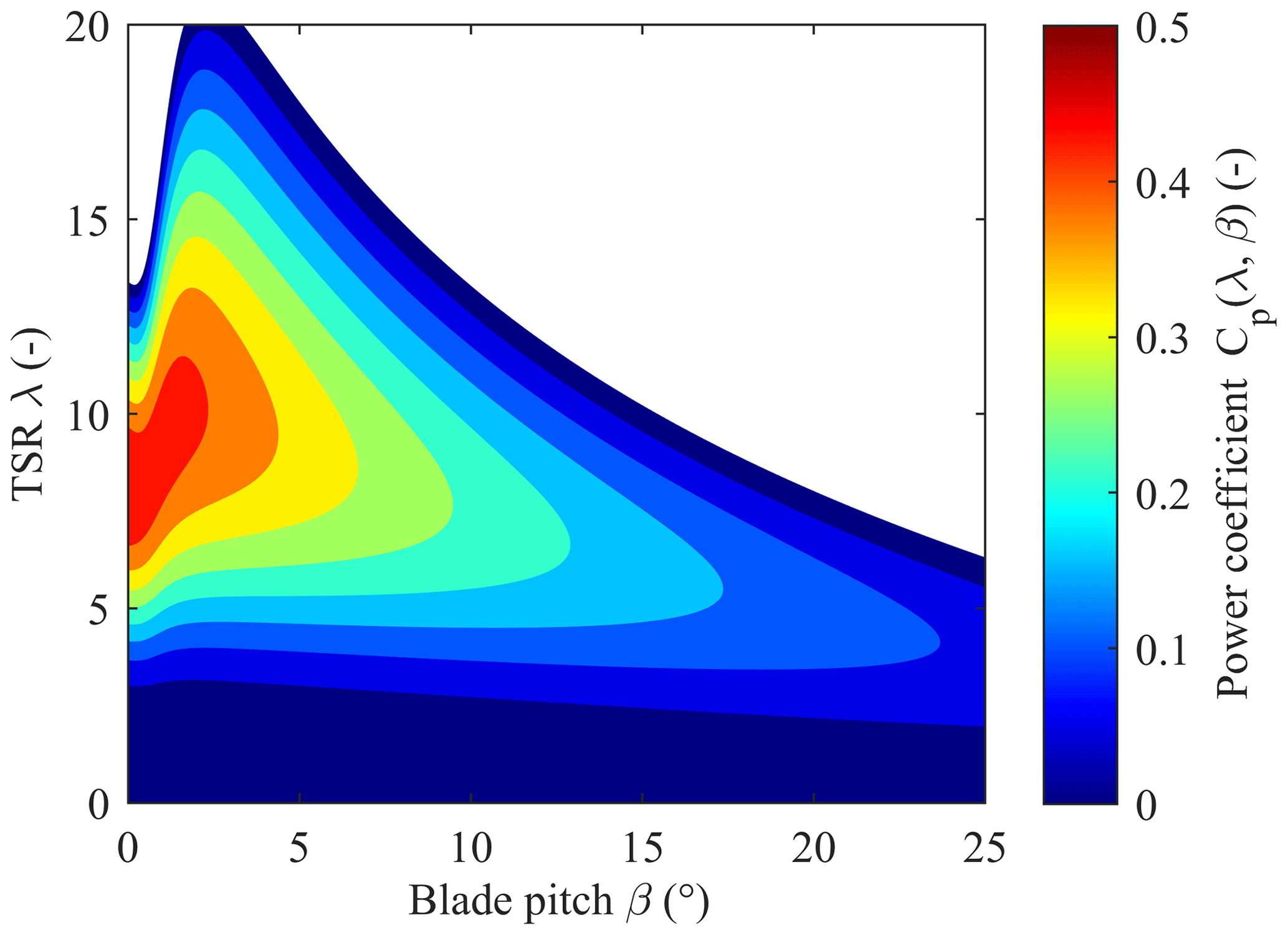
Figure 1 Power coefficient C_p with respect to tip-speed ratio λ and blade pitch angle β (Sarbandi et al., 2025).

2.2 Reduced-order observation-oriented model of a FOWT

The full-order FOWT model includes a high number of degrees of freedom (24) for blade and tower bending modes, platform pitch and surge motions, and mooring dynamics. While this comprehensive model captures detailed turbine behavior, its complexity makes it unsuitable for control design and real-time estimation. Therefore, a reduced-order model is used for observer development. The equation of motion for the rotor speed ω_r is given by

$$\begin{array}{}\text{(5)}& {\dot{\mathit{\omega }}}_{\mathrm{r}}={\displaystyle \frac{\mathrm{1}}{J}}\left({\mathit{\tau }}_{\mathrm{a}}-n_{\mathrm{g}}{\mathit{\tau }}_{\mathrm{g}}\right)+\mathit{\delta }\left(t\right),\end{array}$$

where J is the equivalent rotational inertia, τ_a and τ_g denote the aerodynamic and generator torques respectively, n_g is the gearbox ratio, and δ(⋅) captures unmodeled dynamics and disturbances.

The control vector u consists of the generator torque and the blade pitch angle $\mathit{u}=[{\mathit{\tau }}_{\mathrm{g}}\mathit{\beta }{]}^{\top }$, the input used depending on the operating region (Aslmostafa et al., 2025). In Region II, control is primarily achieved by adjusting the generator torque τ_g, with blade pitch angle fixed at β=0. In contrast, control in Region III is dominated by blade pitch β actuation, with the generator torque τ_g held constant at its rated value; i.e., ${\mathit{\tau }}_{\mathrm{g}}={\mathit{\tau }}_{\mathrm{g}}^{*}$. The objective in this paper is to design an observation solution allowing for the estimation of the REWS v_r from the measurement of the rotor speed ω_r. The wind speed here is viewed as a time-varying parameter whose dynamics are unknown, which gives

$$\begin{array}{}\text{(6)}& {\dot{v}}_{\mathrm{r}}=f_v\left(t\right),\end{array}$$

with f_v(t) being an unknown bounded function. Using ${\mathit{\omega }}_{\mathrm{r}}=\left(\mathit{\lambda }{v}_{\mathrm{r}}\right)/R$ from Eq. (4) together with Eqs. (5)–(6), the observer-based model reads as

$$\begin{array}{}\text{(7)}& \begin{array}{lc}\left[\begin{array}{c}{\dot{\mathit{\omega }}}_{\mathrm{r}}\\ {\dot{v}}_{\mathrm{r}}\end{array}\right]& =\underset{\mathit{f}(\mathit{x},\mathit{u})}{\underbrace{\left[\begin{array}{c}\frac{\mathrm{1}}{J}\left(\frac{\mathit{\rho }\mathit{\pi }{R}^{\mathrm{3}}{v}_{\mathrm{r}}^{\mathrm{2}}}{\mathrm{2}\mathit{\lambda }}{C}_{\mathrm{p}}(\mathit{\lambda },\mathit{\beta })-n_{\mathrm{g}}{\mathit{\tau }}_{\mathrm{g}}\right)\\ \mathrm{0}\end{array}\right]}}\\ & +\underset{\mathrm{\Delta }\left(t\right)}{\underbrace{\left[\begin{array}{c}\mathit{\delta }\left(t\right)\\ f_v\left(t\right)\end{array}\right]}},\end{array}\end{array}$$

with the objective being to estimate v_r from the measurement of ω_r in spite of Δ(⋅). The system can be written in observation-oriented form

$$\begin{array}{}\text{(8)}& \begin{array}{lll}\dot{\mathit{x}}& =& \mathit{f}(\mathit{x},\mathit{u})+\mathrm{\Delta }\left(t\right)\\ y& =& h\left(\mathit{x}\right),\end{array}\end{array}$$

where $\mathit{x}=[{\mathit{\omega }}_{\mathrm{r}}{v}_{\mathrm{r}}{]}^{\top }$ is the state vector, h(x)=ω_r is the measured output, and $\mathit{u}=[{\mathit{\tau }}_{\mathrm{g}}\mathit{\beta }{]}^{\top }$.

• Remark 1. The modeling of C_p(λ,β) has been carried out extensively (Castillo et al., 2023). In this study, an exponential model is used that approximates the power coefficient and reads as

  $$\begin{array}{}\text{(9)}& C_{\mathrm{p}}(\mathit{\lambda },\mathit{\beta })\approx a(\mathit{\lambda },\mathit{\beta })\mathit{\beta }+b(\mathit{\lambda },\mathit{\beta }),\end{array}$$

  where the coefficients a and b are defined as

  $$\begin{array}{}\text{(10)}& {\displaystyle }\begin{array}{rl}a& =-c_{\mathrm{0}}{c}_{\mathrm{2}}\exp (-c_{\mathrm{4}}{\mathit{\lambda }}_{\mathrm{1}}^{-\mathrm{1}}),\\ b& =c_{\mathrm{0}}(c_{\mathrm{1}}{\mathit{\lambda }}_{\mathrm{1}}^{-\mathrm{1}}-c_{\mathrm{3}})\exp (-c_{\mathrm{4}}{\mathit{\lambda }}_{\mathrm{1}}^{-\mathrm{1}}),\end{array}\end{array}$$

  with

  $${\mathit{\lambda }}_{\mathrm{1}}^{-\mathrm{1}}={\displaystyle \frac{\mathrm{1}}{\mathit{\lambda }+c_{\mathrm{5}}\mathit{\beta }}}-{\displaystyle \frac{c_{\mathrm{6}}}{{\mathit{\beta }}^{\mathrm{3}}+\mathrm{1}}}$$

  and c₀=0.5, c₁=73.5, c₂=0.4, c₃=5, c₄=13.125, c₅=0.08, and c₆=0.0035.

• Remark 2. In the case of FOWTs, platform motions and mooring dynamics are not taken into account in Eq. (8). The proposed estimation methods in the paper are developed on this simplified system and can then be applied to floating (or not) offshore (or not) wind turbines. In the sequel, the observation solutions for estimating the REWS v_r are validated by supposing that only the rotor speed ω_r is measured and through two separate steps: first using the full-order OpenFAST simulator and then the experimental setup. This two-stage evaluation emphasizes the observer's robustness versus simplification of the model.

3 Supertwisting-based observer

Ideally, to achieve high performance in the state/parameter estimation, having an accurate model of the system is a key point. However, modeling the exact dynamics of FOWTs is highly challenging. Therefore, it is crucial to develop estimation methods that are sufficiently robust against system perturbations and modeling uncertainties. In this section, a robust observer based on the supertwisting algorithm (Levant, 1993) is presented for estimating REWS using rotor speed measurement; this observer is based on the reduced-order model presented in the previous section. Additionally, the novelty of the proposed estimation algorithm lies in the fact that the gains are dynamically adapted, allowing for easier tuning.

• Assumption 1. The REWS v_r(t) is assumed to be unmeasured and dynamically unknown. Nevertheless, v_r(t) remains bounded and positive for all t≥0 such that

  $$\begin{array}{}\text{(11)}& \mathrm{0}<v_{\mathrm{r}}\left(t\right)<V_{max}\forall t\ge \mathrm{0},\end{array}$$

  where $V_{max}>\mathrm{0}$ is a constant that represents an upper bound within the turbine's operational regions.

Given the uncertain nature of the system described in Eq. (8), an observer inspired by Shtessel et al. (2014) is proposed. However, the first step is to analyze the observability of Eq. (8) in the operational domain, possibly detecting singularities.

3.1 Observability analysis

This section details the numerical procedure for the analysis of the observability of the system in Eq. (8). We denote the operating domain 𝒪⊂IR⁴ in which $\mathit{x}=[{\mathit{\omega }}_{\mathrm{r}}{v}_{\mathrm{r}}{]}^{\top }$ and $\mathit{u}=[{\mathit{\tau }}_{\mathrm{g}}\mathit{\beta }{]}^{\top }$ are physically evolving. All the results detailed in the rest of the paper are verified only in this domain.

• Assumption 2. The perturbation term δ(t) and its derivative are bounded. Furthermore, δ(t) has no influence on the system observability.

Given the previous assumption, the observability analysis developed in the sequel is made for the system in Eq. (8) without perturbation; i.e. δ(t)=0. The generic observability analysis is defined as follows.

• Definition 1 (Krener and Respondek, 1985). Consider the system given by Eq. (8), with $\mathit{x}=[{\mathit{\omega }}_{\mathrm{r}}{v}_{\mathrm{r}}{]}^{\top }$ and $\mathit{u}=[{\mathit{\tau }}_{\mathrm{g}}\mathit{\beta }{]}^{\top }$ evolving in the operating domain 𝒪, and suppose Assumption 2 is fulfilled. Consider that δ(t)=0. The system formulated in Eq. (8) is locally observable if

  $$\begin{array}{}\text{(12)}& \begin{array}{rl}{\mathbf{\Phi }}_{\mathit{\delta }\left(t\right)=\mathrm{0}}& ={\left[\begin{array}{c}y\\ \dot{y}\end{array}\right]}_{\mathit{\delta }\left(t\right)=\mathrm{0}}\\ & =\left[\begin{array}{c}{\mathit{\omega }}_{\mathrm{r}}\\ \frac{\mathrm{1}}{J}\left(\frac{\mathit{\rho }\mathit{\pi }{R}^{\mathrm{3}}{v}_{\mathrm{r}}^{\mathrm{2}}}{\mathrm{2}\mathit{\lambda }({\mathit{\omega }}_{\mathrm{r}},v_{\mathrm{r}})}{C}_{\mathrm{p}}\left(\mathit{\lambda }\right({\mathit{\omega }}_{\mathrm{r}},v_{\mathrm{r}}),\mathit{\beta })-n_{\mathrm{g}}{\mathit{\tau }}_{\mathrm{g}}\right)\end{array}\right]\end{array}\end{array}$$

  is a state coordinate transformation; i.e. $\mathit{z}=\mathbf{\Phi }({\mathit{\omega }}_{\mathrm{r}},v_{\mathrm{r}},\mathit{\beta },{\mathit{\tau }}_{\mathrm{g}})$ is invertible on 𝒪.

Checking whether Φ_δ(t)=0 is invertible is difficult in practice; therefore, the previous definition can be reformulated by the next equivalent one.

• Definition 2. Consider the system given by Eq. (8), with $\mathit{x}=[{\mathit{\omega }}_{\mathrm{r}}{v}_{\mathrm{r}}{]}^{\top }$ and $\mathit{u}=[{\mathit{\tau }}_{\mathrm{g}}\mathit{\beta }{]}^{\top }$ evolving in the operating domain 𝒪, and suppose Assumption 2 fulfilled. The system is generically observable on 𝒪 if

  $$\begin{array}{}\text{(13)}& \det \left[{\displaystyle \frac{\partial {\mathbf{\Phi }}_{\mathit{\delta }\left(t\right)=\mathrm{0}}}{\partial \mathit{x}}}\right]\ne \mathrm{0}\end{array}$$

  with

  $$\begin{array}{}\text{(14)}& \begin{array}{rl}{\mathbf{\Phi }}_{\mathit{\delta }\left(t\right)=\mathrm{0}}& ={\left[\begin{array}{c}y\\ \dot{y}\end{array}\right]}_{\mathit{\delta }\left(t\right)=\mathrm{0}}\\ & =\left[\begin{array}{c}{\mathit{\omega }}_{\mathrm{r}}\\ \frac{\mathrm{1}}{J}\left(\frac{\mathit{\rho }\mathit{\pi }{R}^{\mathrm{3}}{v}_{\mathrm{r}}^{\mathrm{2}}}{\mathrm{2}\mathit{\lambda }({\mathit{\omega }}_{\mathrm{r}},v_{\mathrm{r}})}{C}_{\mathrm{p}}\left(\mathit{\lambda }\right({\mathit{\omega }}_{\mathrm{r}},v_{\mathrm{r}}),\mathit{\beta })-n_{\mathrm{g}}{\mathit{\tau }}_{\mathrm{g}}\right)\end{array}\right].\end{array}\end{array}$$

The Jacobian of Φ with respect to the state vector x reads

$$\begin{array}{}\text{(15)}& {\displaystyle \frac{\partial \mathbf{\Phi }}{\partial \mathit{x}}}=\left[\begin{array}{cc}\frac{\partial y}{\partial {\mathit{\omega }}_{\mathrm{r}}}& \frac{\partial y}{\partial v_{\mathrm{r}}}\\ \frac{\partial \dot{y}}{\partial {\mathit{\omega }}_{\mathrm{r}}}& \frac{\partial \dot{y}}{\partial v_{\mathrm{r}}}\end{array}\right]=\left[\begin{array}{cc}\mathrm{1}& \mathrm{0}\\ \frac{\partial \dot{y}}{\partial {\mathit{\omega }}_{\mathrm{r}}}& \frac{\partial \dot{y}}{\partial v_{\mathrm{r}}}\end{array}\right].\end{array}$$

Therefore, the generic observability condition $\det (\partial \mathbf{\Phi }/\partial \mathit{x})\ne \mathrm{0}$ is equivalent to requiring that $\partial \dot{y}/\partial v_{\mathrm{r}}\ne \mathrm{0}$.

• Observability condition. The system defined by Eq. (8) is locally observable if the following condition is fulfilled:

  $$\begin{array}{}\text{(16)}& {\displaystyle \frac{\partial \dot{y}}{\partial v_{\mathrm{r}}}}\ne \mathrm{0}⟺{\displaystyle \frac{\partial C_{\mathrm{p}}}{\partial v_{\mathrm{r}}}}\cdot v_{\mathrm{r}}+\mathrm{3}{C}_{\mathrm{p}}\left(\mathit{\lambda }\right({\mathit{\omega }}_{\mathrm{r}},v_{\mathrm{r}}),\mathit{\beta })\ne \mathrm{0}.\end{array}$$

In the simulation sections, the previous condition in Eq. (16) is numerically and experimentally evaluated in realistic operating conditions.

3.2 Observer design

Consider the system defined by Eq. (8) that is locally observable. As a consequence, the transformation

$$\begin{array}{}\text{(17)}& \mathit{z}=\left[\begin{array}{c}{z}_{\mathrm{1}}\\ z_{\mathrm{2}}\end{array}\right]=\left[\begin{array}{c}y\\ \dot{y}\end{array}\right]=\mathbf{\Phi }({\mathit{\omega }}_{\mathrm{r}},v_{\mathrm{r}},\mathit{\beta },{\mathit{\tau }}_{\mathrm{g}})\end{array}$$

is a state coordinate transformation; i.e. the state vector $\mathit{x}=[{\mathit{\omega }}_{\mathrm{r}}{v}_{\mathrm{r}}{]}^{\top }$ can be expressed as a function of z₁, z₂, τ_g, and β. That is,

$$\begin{array}{}\text{(18)}& \mathit{x}=\left[\begin{array}{c}{\mathit{\omega }}_{\mathrm{r}}\\ v_{\mathrm{r}}\end{array}\right]={\mathbf{\Phi }}^{-\mathrm{1}}(z_{\mathrm{1}},z_{\mathrm{2}},\mathit{\beta },{\mathit{\tau }}_{\mathrm{g}}).\end{array}$$

Furthermore, from the state coordinate transformation given in Eq. (17), one gets

$$\begin{array}{}\text{(19)}& \begin{array}{lcl}{\dot{z}}_{\mathrm{1}}& =& z_{\mathrm{2}}\\ {\dot{z}}_{\mathrm{2}}& =& {\ddot{\mathit{\omega }}}_{\mathrm{r}}=\frac{\mathrm{d}}{\mathrm{d}t}\left[\frac{\mathit{\rho }\mathit{\pi }{R}^{\mathrm{3}}{v}_{\mathrm{r}}^{\mathrm{2}}}{\mathrm{2}J\mathit{\lambda }}{C}_{\mathrm{p}}(\mathit{\lambda },\mathit{\beta })\right]-\frac{n_{\mathrm{g}}}{J}{\dot{\mathit{\tau }}}_{\mathrm{g}}+\dot{\mathit{\delta }}\left(t\right),\end{array}\end{array}$$

which can be rewritten as

$$\begin{array}{}\text{(20)}& \dot{\mathit{z}}=\left[\begin{array}{c}{\dot{z}}_{\mathrm{1}}\\ {\dot{z}}_{\mathrm{2}}\end{array}\right]=\underset{\mathbf{A}}{\underbrace{\left[\begin{array}{cc}\mathrm{0}& \mathrm{1}\\ \mathrm{0}& \mathrm{0}\end{array}\right]}}\mathit{z}+\left[\begin{array}{c}\mathrm{0}\\ \mathcal{F}(\cdot )\end{array}\right],\end{array}$$

with (replacing ω_r and β with the state coordinate transformation in Eq. 18)

$$\begin{array}{}\text{(21)}& \mathcal{F}(\cdot )={\displaystyle \frac{\mathrm{d}}{\mathrm{d}t}}\left[{\displaystyle \frac{\mathit{\rho }\mathit{\pi }{R}^{\mathrm{3}}{v}_{\mathrm{r}}^{\mathrm{2}}}{\mathrm{2}J\mathit{\lambda }}}{C}_{\mathrm{p}}(\mathit{\lambda },\mathit{\beta })\right]-{\displaystyle \frac{n_{\mathrm{g}}}{J}}{\dot{\mathit{\tau }}}_{\mathrm{g}}+\dot{\mathit{\delta }}\left(t\right).\end{array}$$

It should be noted that the structure in Eq. (20) corresponds to a perturbed double-integrator system. Indeed, the coordinate transformation in Eq. (17) yields z₁=y and $z_{\mathrm{2}}=\dot{y}$ so that ${\dot{z}}_{\mathrm{1}}=z_{\mathrm{2}}$. All model uncertainties and unmeasured effects appear as an additive term in the second equation, namely ${\dot{z}}_{\mathrm{2}}=\mathcal{F}(\cdot )$. Therefore, the linear part of the dynamics corresponds to the standard chain-of-integrators form.

• Assumption 3. The time derivatives of the control inputs (i.e., $\dot{\mathit{\beta }}$ and ${\dot{\mathit{\tau }}}_{\mathrm{g}}$) are bounded over the operating domain 𝒪. The function ℱ(⋅), which involves ${\dot{v}}_{\mathrm{r}}$ and $\dot{\mathit{\delta }}\left(t\right)$, is unknown but is assumed to be bounded over 𝒪.

Given that the function ℱ(⋅) is not well-known, it cannot appear in the observer. A solution for the observation of the system defined by Eq. (20) is a robust one proposed by Levant (2003). Thus, consider the canonical form in Eq. (20) that is a perturbed uncertain double integrator. From Levant (2003), the supertwisting-based observer reads as

$$\begin{array}{}\text{(22)}& \begin{array}{lcl}{\dot{\widehat{z}}}_{\mathrm{1}}& =& {\widehat{z}}_{\mathrm{2}}+\underset{{\mathit{\gamma }}_{\mathrm{1}}(z_{\mathrm{1}},{\widehat{z}}_{\mathrm{1}})}{\underbrace{L_{{\mathit{\varphi }}_{\mathrm{1}}}^{\mathrm{1}/\mathrm{2}}{a}_{\mathrm{1}}{\left|z_{\mathrm{1}}-{\widehat{z}}_{\mathrm{1}}\right|}^{\mathrm{1}/\mathrm{2}}\mathrm{sign}(z_{\mathrm{1}}-{\widehat{z}}_{\mathrm{1}})}}\\ {\dot{\widehat{z}}}_{\mathrm{2}}& =& \underset{{\mathit{\gamma }}_{\mathrm{2}}(z_{\mathrm{1}},{\widehat{z}}_{\mathrm{1}})}{\underbrace{L_{{\mathit{\varphi }}_{\mathrm{1}}}{a}_{\mathrm{2}}\mathrm{sign}(z_{\mathrm{1}}-{\widehat{z}}_{\mathrm{1}})}}\end{array},\end{array}$$

where a₁ and a₂ are constant values that are fixed as suggested in Levant (2003), a₁=1.5 and a₂=1.1. Additionally,

$$\begin{array}{}\text{(23)}& L_{{\mathit{\varphi }}_{\mathrm{1}}}>\left|\mathcal{F}(z_{\mathrm{1}},z_{\mathrm{2}},\mathit{\beta },\dot{\mathit{\beta }},{\mathit{\tau }}_g,{\dot{\mathit{\tau }}}_g,t)\right|\end{array}$$

ensures $\widehat{\mathit{z}}=[{\widehat{z}}_{\mathrm{1}}{\widehat{z}}_{\mathrm{2}}{]}^{\top }\to [z_{\mathrm{1}}{z}_{\mathrm{2}}{]}^{\top }$ in a finite time in spite of the perturbations and uncertainties.

• Theorem 1. Consider the system in Eq. (8) and Assumptions 1–3 fulfilled. Suppose that it is locally observable in the sense of Definition 1. Therefore, the system (with Φ defined by Eq. 17)

  $$\begin{array}{}\text{(24)}& \begin{array}{rl}{\displaystyle }\dot{\widehat{\mathit{x}}}& {\displaystyle }=\left[\begin{array}{c}{\dot{\widehat{\mathit{\omega }}}}_{\mathrm{r}}\\ {\dot{\widehat{v}}}_{\mathrm{r}}\end{array}\right]=\mathit{f}(\widehat{\mathit{x}},\mathit{u})+{\left[{\displaystyle \frac{\partial \mathbf{\Phi }}{\partial \widehat{\mathit{x}}}}\right]}^{-\mathrm{1}}\\ {\displaystyle }& {\displaystyle }\cdot \left[\begin{array}{c}{L}_{{\mathit{\varphi }}_{\mathrm{1}}}^{\mathrm{1}/\mathrm{2}}{a}_{\mathrm{1}}|{\mathit{\omega }}_{\mathrm{r}}-{\widehat{\mathit{\omega }}}_{\mathrm{r}}{|}^{\mathrm{1}/\mathrm{2}}\mathrm{sign}({\mathit{\omega }}_{\mathrm{r}}-{\widehat{\mathit{\omega }}}_{\mathrm{r}})\\ L_{{\mathit{\varphi }}_{\mathrm{1}}}{a}_{\mathrm{2}}\mathrm{sign}({\mathit{\omega }}_{\mathrm{r}}-{\widehat{\mathit{\omega }}}_{\mathrm{r}})\end{array}\right]\end{array}\end{array}$$

  is an observer of Eqs. (7)–(8) with a₁ and a₂ being constant values that are fixed as suggested in Levant (2003), a₁=1.5 and a₂=1.1, and the constant $L_{{\mathit{\varphi }}_{\mathrm{1}}}$ such that

  $$\begin{array}{}\text{(25)}& L_{{\mathit{\varphi }}_{\mathrm{1}}}>\left|{\displaystyle \frac{\mathrm{d}}{\mathrm{d}t}}\left[{\displaystyle \frac{\mathit{\rho }\mathit{\pi }{R}^{\mathrm{3}}{v}_{\mathrm{r}}^{\mathrm{2}}}{\mathrm{2}J\mathit{\lambda }}}{C}_{\mathrm{p}}(\mathit{\lambda },\mathit{\beta })\right]-{\displaystyle \frac{n_{\mathrm{g}}}{J}}{\dot{\mathit{\tau }}}_{\mathrm{g}}+\dot{\mathit{\delta }}\left(t\right)\right|.\end{array}$$

• Proof of Theorem 1. The observer in Eq. (22) has been designed for the system in Eq. (20) in the $\widehat{\mathit{z}}$ state space; the gain $L_{{\mathit{\varphi }}_{\mathrm{1}}}$ tuning is based on the bound of ℱ(⋅). From there, the writing of the observer in Eq. (22) must be made in the $\widehat{\mathit{x}}$ state space. With this objective, consider $\mathit{z}=\mathbf{\Phi }(\mathit{x},\mathit{u})$ that gives

  $$\begin{array}{}\text{(26)}& \dot{\mathit{z}}={\displaystyle \frac{\partial \mathbf{\Phi }}{\partial \mathit{x}}}\dot{\mathit{x}}+{\displaystyle \frac{\partial \mathbf{\Phi }}{\partial \mathit{u}}}\dot{\mathit{u}}.\end{array}$$

  Therefore, one has

  $$\begin{array}{}\text{(27)}& \mathbf{A}\cdot \mathit{z}+\left[\begin{array}{c}\mathrm{0}\\ \mathcal{F}\end{array}\right]={\displaystyle \frac{\partial \mathbf{\Phi }}{\partial \mathit{x}}}\mathit{f}(\mathit{x},\mathit{u})+{\displaystyle \frac{\partial \mathbf{\Phi }}{\partial \mathit{u}}}\dot{\mathit{u}}+{\displaystyle \frac{\partial \mathbf{\Phi }}{\partial \mathit{x}}}\mathrm{\Delta }\left(t\right).\end{array}$$

  By considering non-perturbed and perturbed terms in the two state spaces, one has

  $$\begin{array}{}\text{(28)}& \mathbf{A}\cdot \mathit{z}={\displaystyle \frac{\partial \mathbf{\Phi }}{\partial \mathit{x}}}\mathit{f}(\mathit{x},\mathit{u})+{\displaystyle \frac{\partial \mathbf{\Phi }}{\partial \mathit{u}}}\dot{\mathit{u}}\mathrm{and}\left[\begin{array}{c}\mathrm{0}\\ \mathcal{F}\end{array}\right]={\displaystyle \frac{\partial \mathbf{\Phi }}{\partial \mathit{x}}}\mathrm{\Delta }\left(t\right).\end{array}$$

  From $\widehat{\mathit{z}}=\mathbf{\Phi }(\widehat{\mathit{x}},\mathit{u})$, an observer of Eq. (22) in the $\widehat{\mathit{x}}$ state space reads as

  $$\begin{array}{}\text{(29)}& \begin{array}{lcl}\dot{\widehat{\mathit{x}}}& =& {\left[\frac{\partial \mathbf{\Phi }}{\partial \widehat{\mathit{x}}}\right]}^{-\mathrm{1}}\cdot \left(\dot{\widehat{\mathit{z}}}-\frac{\partial \mathbf{\Phi }}{\partial \mathit{u}}\dot{\mathit{u}}\right)\\ & =& {\left[\frac{\partial \mathbf{\Phi }}{\partial \widehat{\mathit{x}}}\right]}^{-\mathrm{1}}\cdot \left(\mathbf{A}\widehat{\mathit{z}}+\left[\begin{array}{c}{\mathit{\gamma }}_{\mathrm{1}}(\cdot )\\ {\mathit{\gamma }}_{\mathrm{2}}(\cdot )\end{array}\right]-\frac{\partial \mathbf{\Phi }}{\partial \mathit{u}}\dot{\mathit{u}}\right)\\ & =& {\left[\frac{\partial \mathbf{\Phi }}{\partial \widehat{\mathit{x}}}\right]}^{-\mathrm{1}}\cdot \left(\mathbf{A}\widehat{\mathit{z}}-\frac{\partial \mathbf{\Phi }}{\partial \mathit{u}}\dot{\mathit{u}}\right)+{\left[\frac{\partial \mathbf{\Phi }}{\partial \widehat{\mathit{x}}}\right]}^{-\mathrm{1}}\cdot \left[\begin{array}{c}{\mathit{\gamma }}_{\mathrm{1}}(\cdot )\\ {\mathit{\gamma }}_{\mathrm{2}}(\cdot )\end{array}\right].\end{array}\end{array}$$

  From the left-hand side term of Eq. (28), the previous system reads as

  $$\begin{array}{}\text{(30)}& \dot{\widehat{\mathit{x}}}=\mathit{f}(\widehat{\mathit{x}},\mathit{u})+{\left[{\displaystyle \frac{\partial \mathbf{\Phi }}{\partial \widehat{\mathit{x}}}}\right]}^{-\mathrm{1}}\cdot \left[\begin{array}{c}{\mathit{\gamma }}_{\mathrm{1}}(\cdot )\\ {\mathit{\gamma }}_{\mathrm{2}}(\cdot )\end{array}\right],\end{array}$$

  which is the form of the system displayed in Theorem 1. Given that the system in Eq. (22) is an observer of Eq. (20) under the condition in Eq. (23), then the system in Eq. (29) is an observer for Eq. (8) if the condition in Eq. (25) is fulfilled with a₁=1.5 and a₂=1.1.

3.3 Adaptive observer gain

A drawback of the proposed approach is that the term $L_{{\mathit{\varphi }}_{\mathrm{1}}}$ is difficult to carefully tune because determining the bound of

$$\begin{array}{}\text{(31)}& \left|{\displaystyle \frac{\mathrm{d}}{\mathrm{d}t}}\left[{\displaystyle \frac{\mathit{\rho }\mathit{\pi }{R}^{\mathrm{3}}{v}_{\mathrm{r}}^{\mathrm{2}}}{\mathrm{2}J\mathit{\lambda }}}{C}_{\mathrm{p}}(\mathit{\lambda },\mathit{\beta })\right]-{\displaystyle \frac{n_{\mathrm{g}}}{J}}{\dot{\mathit{\tau }}}_{\mathrm{g}}+\dot{\mathit{\delta }}\left(t\right)\right|\end{array}$$

is a very hard task that could give an overestimation and then induce chattering. A solution consists of using an adaptive version of the supertwisting-based observer (Mirzaei et al., 2022), which allows online tuning of the observer thanks to the evaluation on only the estimation error of ω_r. The principle is the following:

• If the estimation error of ω_r is large, it could be due to gains that are too small versus the uncertainty/perturbation effects. Then, gain adaptation law is defined in order to increase the gains of the observers.

• In the opposite case, i.e. if the estimation error of ω_r is small, it means that the observer gains are large enough. Then, gain adaptation law is defined in order to reduce them.

Therefore, the observer in Eq. (24) is replaced by its adaptive version, reading as (Mirzaei et al., 2022)

$$\begin{array}{}\text{(32)}& \begin{array}{rl}\dot{\widehat{\mathit{x}}}& =\left[\begin{array}{c}{\dot{\widehat{\mathit{\omega }}}}_{\mathrm{r}}\\ {\dot{\widehat{v}}}_{\mathrm{r}}\end{array}\right]=\mathit{f}(\widehat{\mathit{x}},\mathit{u})+{\left[{\displaystyle \frac{\partial \mathbf{\Phi }}{\partial \widehat{\mathit{x}}}}\right]}^{-\mathrm{1}}\\ & \cdot \left[\begin{array}{c}{k}_{\mathrm{1}}{\left|{\mathit{\omega }}_{\mathrm{r}}-{\widehat{\mathit{\omega }}}_{\mathrm{r}}\right|}^{\mathrm{1}/\mathrm{2}}\mathrm{sign}({\mathit{\omega }}_{\mathrm{r}}-{\widehat{\mathit{\omega }}}_{\mathrm{r}})\\ k_{\mathrm{2}}\mathrm{sign}({\mathit{\omega }}_{\mathrm{r}}-{\widehat{\mathit{\omega }}}_{\mathrm{r}})\end{array}\right],\end{array}\end{array}$$

with

$$\begin{array}{}\text{(33)}& {\displaystyle }{\dot{k}}_{\mathrm{1}}& {\displaystyle }=\left\{\begin{array}{ll}{\displaystyle \frac{\mathit{\alpha }}{\left|\mathit{\psi }\right|+\mathit{\epsilon }}},{\displaystyle \frac{\mathit{\alpha }}{\mathrm{2}|{\mathit{\omega }}_{\mathrm{r}}-{\widehat{\mathit{\omega }}}_{\mathrm{r}}{|}^{\mathrm{1}/\mathrm{2}}}},& \text{if }|{\mathit{\omega }}_{\mathrm{r}}-{\widehat{\mathit{\omega }}}_{\mathrm{r}}|>\mathit{\epsilon },\\ -k_{\mathrm{1}},{\displaystyle \frac{\mathit{\alpha }}{\mathrm{2}|{\mathit{\omega }}_{\mathrm{r}}-{\widehat{\mathit{\omega }}}_{\mathrm{r}}{|}^{\mathrm{1}/\mathrm{2}}}},& \text{if }|{\mathit{\omega }}_{\mathrm{r}}-{\widehat{\mathit{\omega }}}_{\mathrm{r}}|\le \mathit{\epsilon },\end{array}\right.\text{(34)}& {\displaystyle }{\dot{k}}_{\mathrm{2}}& {\displaystyle }=\left\{\begin{array}{ll}{\displaystyle \frac{\mathit{\alpha }}{\mathrm{2}|{\mathit{\omega }}_{\mathrm{r}}-{\widehat{\mathit{\omega }}}_{\mathrm{r}}{|}^{\mathrm{1}/\mathrm{2}}}},& \text{if }|{\mathit{\omega }}_{\mathrm{r}}-{\widehat{\mathit{\omega }}}_{\mathrm{r}}|>\mathit{\epsilon },\\ -k_{\mathrm{2}},{\displaystyle \frac{\mathit{\alpha }}{\mathrm{2}|{\mathit{\omega }}_{\mathrm{r}}-{\widehat{\mathit{\omega }}}_{\mathrm{r}}{|}^{\mathrm{1}/\mathrm{2}}}},& \text{if }|{\mathit{\omega }}_{\mathrm{r}}-{\widehat{\mathit{\omega }}}_{\mathrm{r}}|\le \mathit{\epsilon },\end{array}\right.\end{array}$$

with $\mathit{\psi }=\frac{\mathrm{d}}{\mathrm{d}t}({\mathit{\omega }}_{\mathrm{r}}-{\widehat{\mathit{\omega }}}_{\mathrm{r}})$, where α>0 and ε>0 are design parameters of the adaptive law. The parameter ε defines the target accuracy of the rotor speed estimation, while α governs the adaptation rate of the observer gains. The constants k₁(0)>0 and k₂(0)>0 denote the initial values of the adaptive gains.
The adaptation mechanism operates according to the following principle: (i) when the estimation error exceeds the target accuracy, i.e., $|{\mathit{\omega }}_{\mathrm{r}}-{\widehat{\mathit{\omega }}}_{\mathrm{r}}|>\mathit{\epsilon }$, the observer gains are increased to improve convergence, and (ii) when the estimation accuracy is sufficient, the gains are decreased to avoid unnecessary amplification of measurement noise.

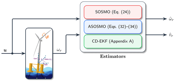
In Fig. 2, the overall estimation framework is illustrated. The rotor speed ω_r is the only measured signal, whereas the generator torque τ_g and the blade pitch angle β serve as known control inputs. These quantities are used within a reduced-order, observation-oriented model (Sect. 2), upon which three estimators are implemented: the SOSMO, its adaptive version ASOSMO, and the CD–EKF. Each estimator provides estimates of both the REWS ${\widehat{v}}_{\mathrm{r}}$ and the rotor speed ${\widehat{\mathit{\omega }}}_{\mathrm{r}}$. The CD–EKF serves as a benchmark for assessing the performance of the proposed sliding-mode estimators.

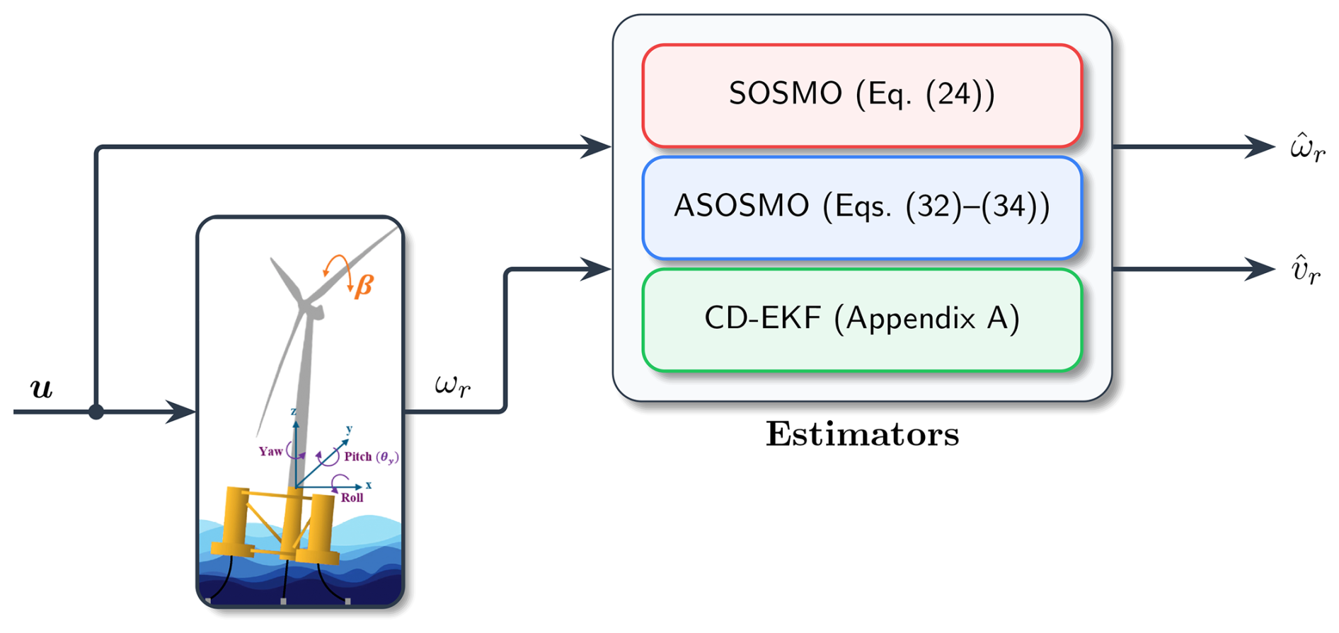
Figure 2 Overview of the estimator architecture proposed in this work, in which the rotor speed ω_r is the only measured signal. The outputs ${\widehat{v}}_{\mathrm{r}}$ and ${\widehat{\mathit{\omega }}}_{\mathrm{r}}$ denote the estimated REWS and rotor speeds, respectively.

4 Simulation results

In this section, the performances of the proposed wind speed observers are evaluated and compared with the CD–EKF used in ROSCO, which is described in Appendix A. All simulations are conducted on the NREL 5 MW FOWT, supported by a semi-submersible platform. The simulation study in this section is conducted in the above-rated operating regime (Region III). Other operating regimes are covered in the experimental validation section (Sect. 5).

4.1 Simulation setup

The simulation environment integrates MATLAB/Simulink (2023a) for implementing the observers with OpenFAST (Jonkman et al., 2009), which simulates the high-fidelity aero-hydro-servo-elastic model of the FOWT. Each test is run for 800 s under identical wind and wave conditions, with a fixed sampling time of 0.0125 s. Although the observer design is based on the reduced-order model in Eq. (5), all 24 degrees of freedom available in OpenFAST are activated to ensure a comprehensive evaluation under realistic conditions.

Realistic turbulent inflow wind fields are generated using TurbSim (Jonkman, 2009) based on the IEC Kaimal turbulence model, with a mean wind speed of 18 m s⁻¹. A logarithmic mean wind profile is employed, resulting in vertical wind shear across the rotor disk. The inflow is prescribed as a full-field turbulent wind to OpenFAST such that the aerodynamic loads are computed using the spatially varying wind field. For analysis and validation purposes, REWS is considered, while the underlying aerodynamic response is influenced by the full-field inflow. Irregular wave conditions are modeled using the HydroDyn module (Jonkman et al., 2014). The incident wave field is prescribed as a stochastic irregular process with a significant wave height of 3.25 m. Hydrodynamic loads acting on the floating platform are computed using the built-in potential-flow formulation in HydroDyn, based on precomputed WAMIT data. This formulation accounts for linear wave-excitation forces, hydrostatic restoring forces, and radiation effects through convolution-based memory terms. The hydrodynamic model is fully coupled with the aero-servo-elastic dynamics in OpenFAST such that wave-induced platform motions interact with the aerodynamic response of the rotor. Both wind and wave conditions are illustrated in Fig. 3. The observer design parameters have been fine-tuned to achieve the best performance as follows: for the constant-gain SOSMO in Eq. (24), the coefficients are set following Levant (2003) to a₁=1.5 and a₂=1.1, and the gain is selected as $L_{{\mathit{\varphi }}_{\mathrm{1}}}=\mathrm{0.01}$; for the adaptive-gain observer (ASOSMO) in Eqs. (32)–(34), the design parameters are chosen as $\mathit{\alpha }={\mathrm{10}}^{-\mathrm{4}}$ and $\mathit{\epsilon }={\mathrm{10}}^{-\mathrm{3}}$, with initial values of k₁(0)=0.1 and $k_{\mathrm{2}}\left(\mathrm{0}\right)={\mathrm{10}}^{-\mathrm{4}}$.

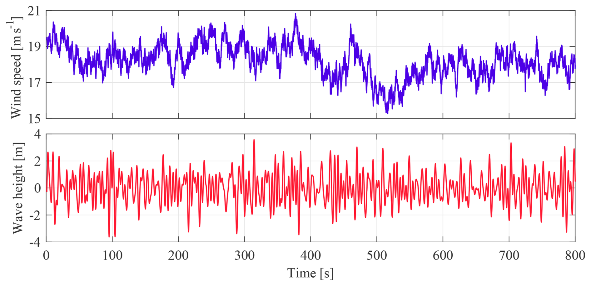
Figure 3 Environmental conditions used in the simulations: turbulent wind speed (top) generated by TurbSim and irregular wave elevation (bottom) generated by the HydroDyn module.

4.2 Results and analysis

Prior to evaluating the performances of observers, the system's observability is verified from Eq. (16). Figure 4 illustrates the evolution of Eq. (16). Its consistently nonzero behavior confirms that Φ is invertible, thereby ensuring observability of the nonlinear system under stochastic wind conditions.

Figure 4 Time evolution of the observability condition given in Eq. (16).

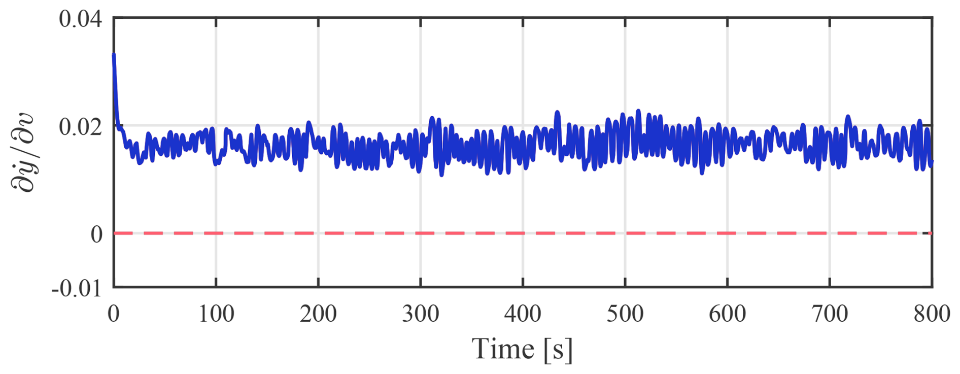
With the observability condition satisfied in Fig. 4, the estimation performance of the three observers in Fig. 2 is subsequently assessed.

4.2.1 Second-order sliding-mode observer (SOSMO)

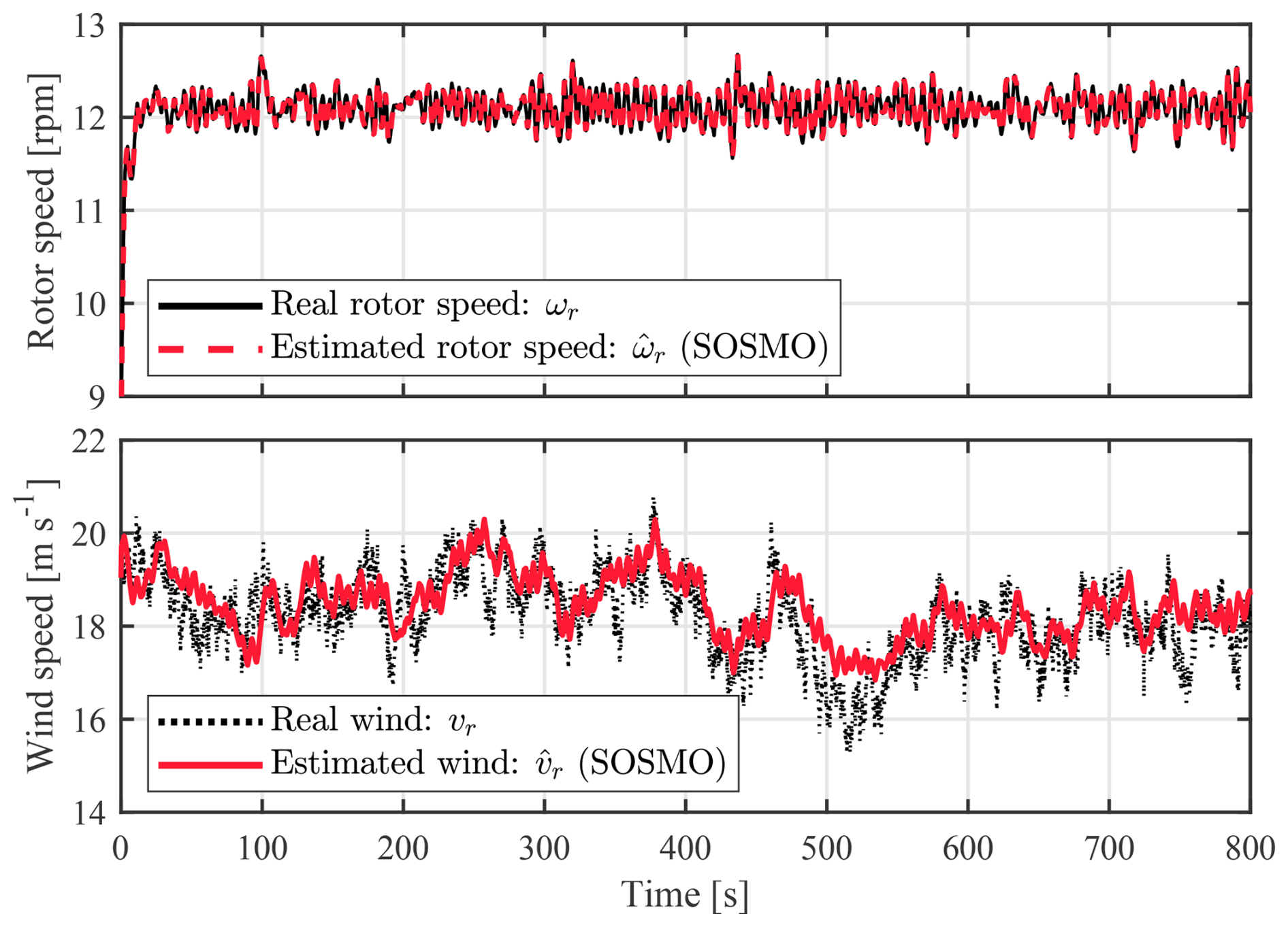
Figure 5 shows the rotor speed and wind speed estimation results for the SOSMO. Despite its relatively simple structure, the SOSMO achieves acceptable estimation performance. A notable property in Fig. 5 is the filtering effect of the SOSMO compared with the measured wind speed.

Figure 5 Rotor speed (above) and wind speed (bottom) estimation results of SOSMO defined in Eq. (24).

4.2.2 Adaptive second-order sliding-mode observer (ASOSMO)

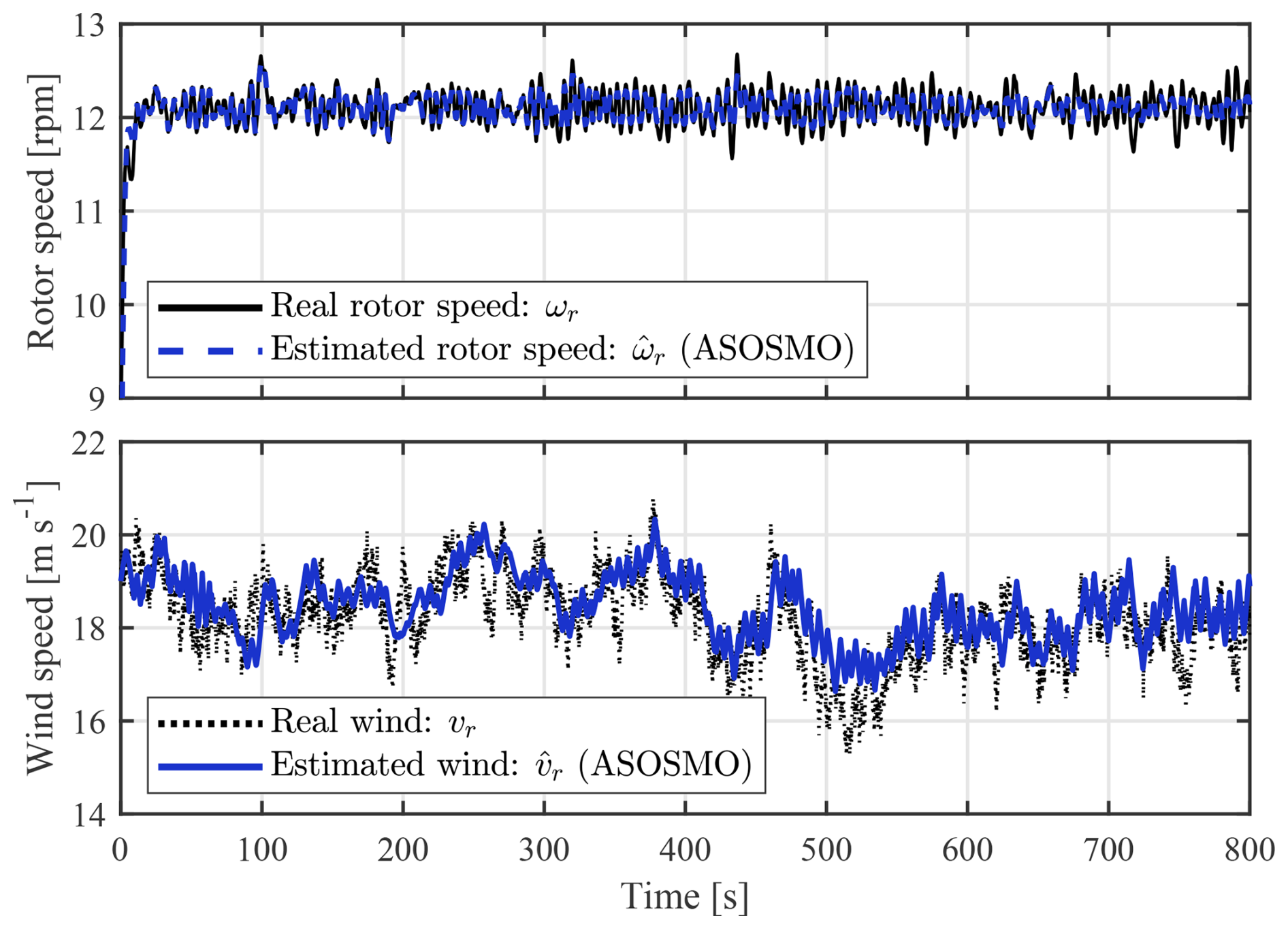
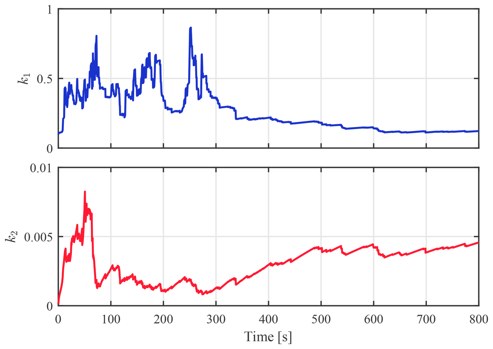
Figure 6 presents the rotor speed and wind speed estimation results of ASOSMO. The distinguishing feature of ASOSMO is its ability to adapt observer gains online, which enhances robustness against model uncertainties and time-varying operating conditions. Unlike the previous SOSMO that relies on fixed gains, ASOSMO continuously adjusts its gains based on real-time system behavior, reducing the dependence on accurate prior model knowledge. As illustrated in Fig. 7, the adaptive gains evolve dynamically during the estimation process, responding effectively to state variations.

Figure 6 Rotor speed (above) and wind speed (bottom) estimation results of ASOSMO defined in Eqs. (32)–(34).

Figure 7 Evolution of adaptation gains k₁ (top) and k₂ (bottom) in ASOSMO in Eqs. (32)–(34).

4.2.3 Continuous–discrete extended Kalman filter (CD–EKF)

Figure 8 presents the rotor speed and wind speed estimation results obtained using the CD–EKF. Under the considered operating conditions, the CD–EKF provides smooth estimates of both quantities and serves as a widely adopted benchmark in wind turbine control applications.

Figure 8 Rotor speed (above) and wind speed (bottom) estimation results of CD–EKF.

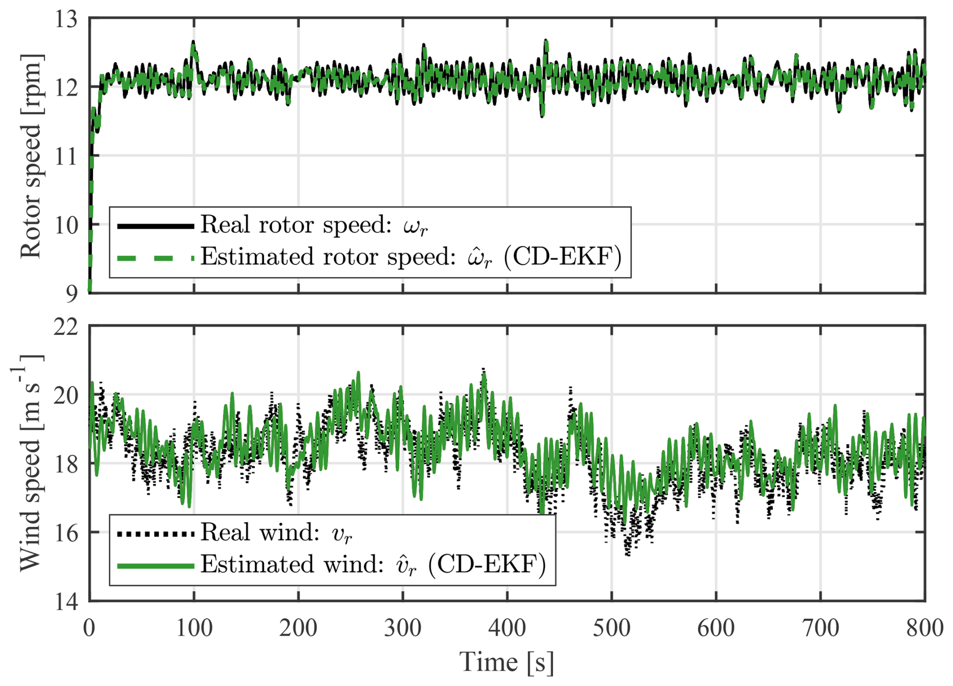
The practical implementation of the CD–EKF requires careful tuning of the process-noise and measurement-noise covariance matrices Q and R_m, which constitute the main design parameters of the filter, as well as linearization of the system dynamics. In the present formulation (see Appendix A), this corresponds to tuning four parameters, namely the diagonal entries of Q associated with the rotor speed state, the turbulent-wind component, and the mean wind component, together with the measurement-noise variance R_m. These parameters are selected based on sensor characteristics, turbulence modeling considerations, and empirical adjustments to ensure filter stability and satisfactory estimation performance.

As commonly reported in the literature, the estimation performance of EKF-based approaches is sensitive to the choice of these covariance parameters. Moreover, no systematic or universal tuning procedure exists for their selection, which represents a well-known practical limitation of Kalman-filter-based methods, particularly for highly nonlinear and uncertain systems such as FOWT.

A comparative evaluation of all three observers is presented in Table 1. The table reports the wind speed estimation accuracy of the three observers under a turbulent-wind scenario. The performance metric used is the root mean square error of the estimation error (i.e., $v_{\mathrm{r}}-{\widehat{v}}_{\mathrm{r}}$). Both sliding-mode-based estimators demonstrate improved precision, with RMSE values of 0.66 and 0.67, respectively, in contrast to the CD–EKF method, which has an RMSE of 0.77. The SOSMO method demonstrates a relative reduction of approximately 14 % in wind speed RMSE when compared with CD–EKF, whereas ASOSMO exhibits a reduction of about 13 %. The findings illustrate the efficacy of sliding-mode-based observers in enhancing estimation accuracy.

Table 1 Comparison of REWS root mean square estimation error (RMSE) for different estimators.

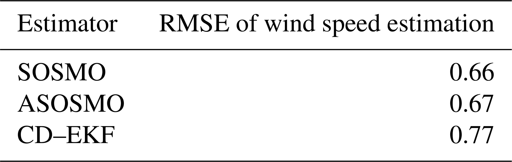
Lower values indicate better estimation performance.

Overall, while all three observers are capable of delivering reliable estimations, SOSMO offers a balance between simplicity and performance. ASOSMO introduces adaptive capability with limited system knowledge, and CD–EKF, though robust, involves a more complex design process. In this context, both the constant-gain and the adaptive versions of SOSMO are considered practical and effective solutions for wind turbine state estimation.

4.3 Monte Carlo analysis

In this subsection, a Monte Carlo (MC) analysis is employed as a powerful tool to assess the sensitivity of the observers to initialization conditions and to quantify their convergence time under identical operating conditions (Sarbandi and Khaloozadeh, 2024).

In this experiment, the only quantity varied from run to run is the initial condition of the observers. All other components of the simulation, including the turbulent wind field, wave excitation, OpenFAST dynamics, and control inputs, are kept identical across all MC realizations. Consequently, any observed variation in transient behavior is solely attributable to different initial observer states. A set of N=100 simulations is generated by initializing the wind and rotor speed estimates within a uniform ±30 % interval around their true values. Three initialization scenarios are examined: (i) rotor speed initialization error only, (ii) wind speed initialization error only, and (iii) simultaneous initialization errors in both wind speed and rotor speed.

To compare the observers consistently, a window convergence time is used. Convergence is declared when the worst-case estimation error across all MC runs remains within a prescribed tolerance band for a continuous duration of T_hold=20 s. The thresholds are chosen as ε_ω=0.2 rpm for rotor speed and ε_v=1.7 m s⁻¹ for wind speed. The convergence time for wind speed is defined as the earliest time at which every MC trajectory satisfies the inequality Δv≤ε_v for all t values in a window of length T_hold. Rotor speed convergence is defined analogously. Requiring convergence over the entire simulation would be unnecessarily restrictive. Turbulent wind excitation, platform motion, and nonlinear aerodynamic effects naturally cause short-lived error fluctuations even after the estimator has converged. The windowed criterion avoids misclassifying such fluctuations as divergence and better reflects practical control requirements.

The resulting convergence times for SOSMO, ASOSMO, and CD–EKF across all scenarios are reported in Table 2 and illustrated in Fig. 9. This metric captures the earliest time after which all realizations remain within the prescribed bounds.

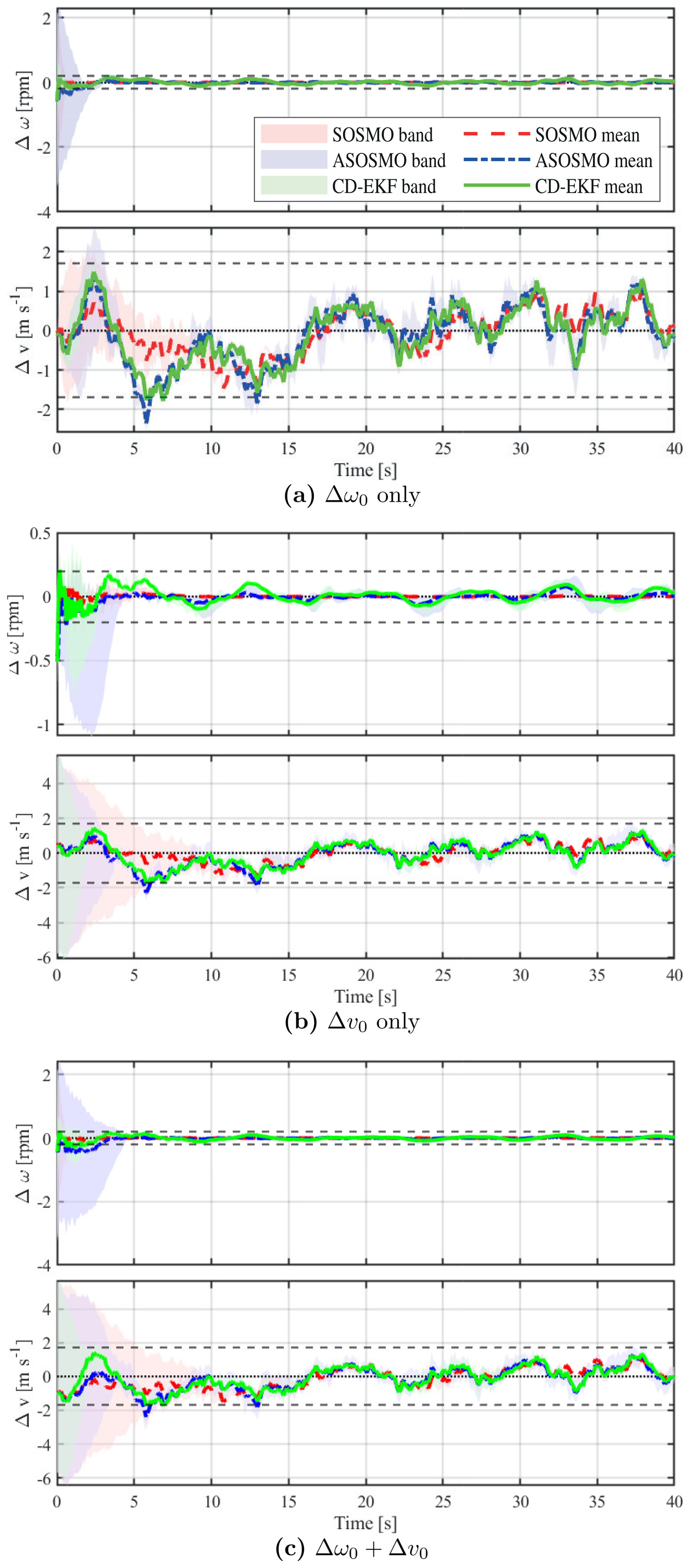
Figure 9 MC analysis with N=100 realizations per scenario for the three initial-condition error cases.

The error-band plots show the dispersion of estimation errors caused solely by changes in initial observer states. In all scenarios, all observers converge. Rotor speed errors settle quickly because ω_r is directly measured, which justifies the smaller threshold ε_ω. Wind speed estimation is more difficult because v_r is unmeasured and its dynamics are unknown. As a result, wind speed error bands are wider, and the threshold ε_v must be larger.

Table 2 Convergence times for rotor speed and wind speed estimation under the three initial-condition initialization scenarios. Each value corresponds to the earliest time at which all MC realizations for N=100 remain within the prescribed error bounds.

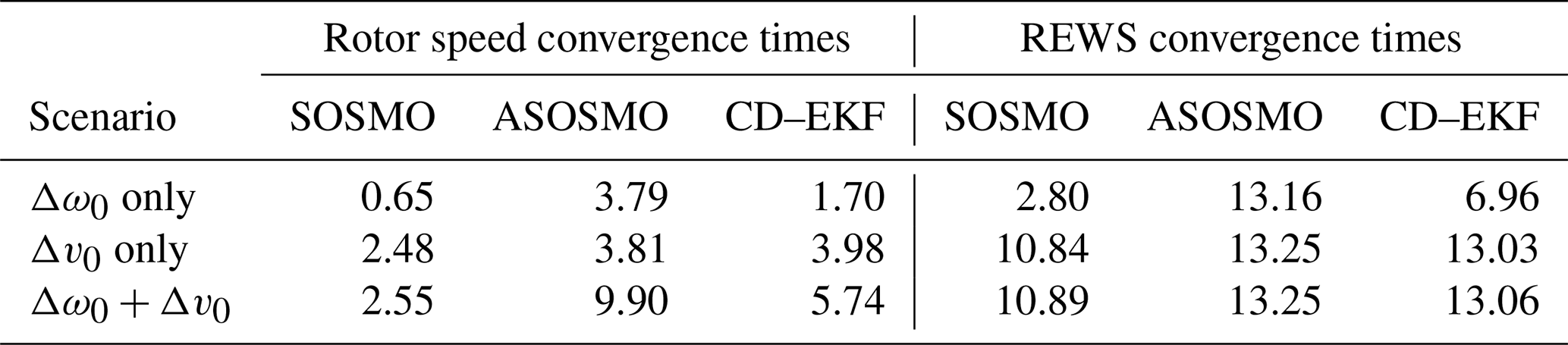
Convergence is declared when all MC realizations remain within the prescribed error bounds for a continuous duration of T_hold=20 s.

From Fig. 9, it can be seen that the CD–EKF typically drives the estimation error toward zero more rapidly during the initial transient. However, when applying the windowed convergence criterion – which requires the estimates to remain within the prescribed bounds for a continuous duration – the SOSMO achieves the shortest convergence times in most scenarios. This difference arises because the adaptive law in the ASOSMO starts with a conservative gain that increases only after sufficient excitation, leading to a slower approach to steady-state accuracy. In contrast, the SOSMO and CD–EKF employ fixed gains or explicit covariance updates, allowing them to settle more quickly once the estimation error enters the tolerance band. Overall, while the CD–EKF is fast in the early transient, the SOSMO exhibits the most favorable worst-case convergence times under the robustness metric used here, whereas the ASOSMO consistently requires longer convergence due to its gain adaptation mechanism.

4.4 Computational time

To assess the computational burden associated with each observer, the execution time of every estimator block using the MATLAB/Simulink Profiler (R2023a) is measured. Importantly, the reported run-time refers exclusively to the time required for the internal computations of each observer. All measurements are obtained under identical conditions (Sect. 4.1), ensuring fair comparison. The CD–EKF exhibited the longest run-time (18 ms), followed by the ASOSMO (11 ms) and the SOSMO (9 ms). These results reflect the higher algorithmic complexity of the CD–EKF, as expected. The ASOSMO increases complexity slightly with its adaptive gain mechanism, in contrast to the constant gain used in the SOSMO (see Fig. 10).

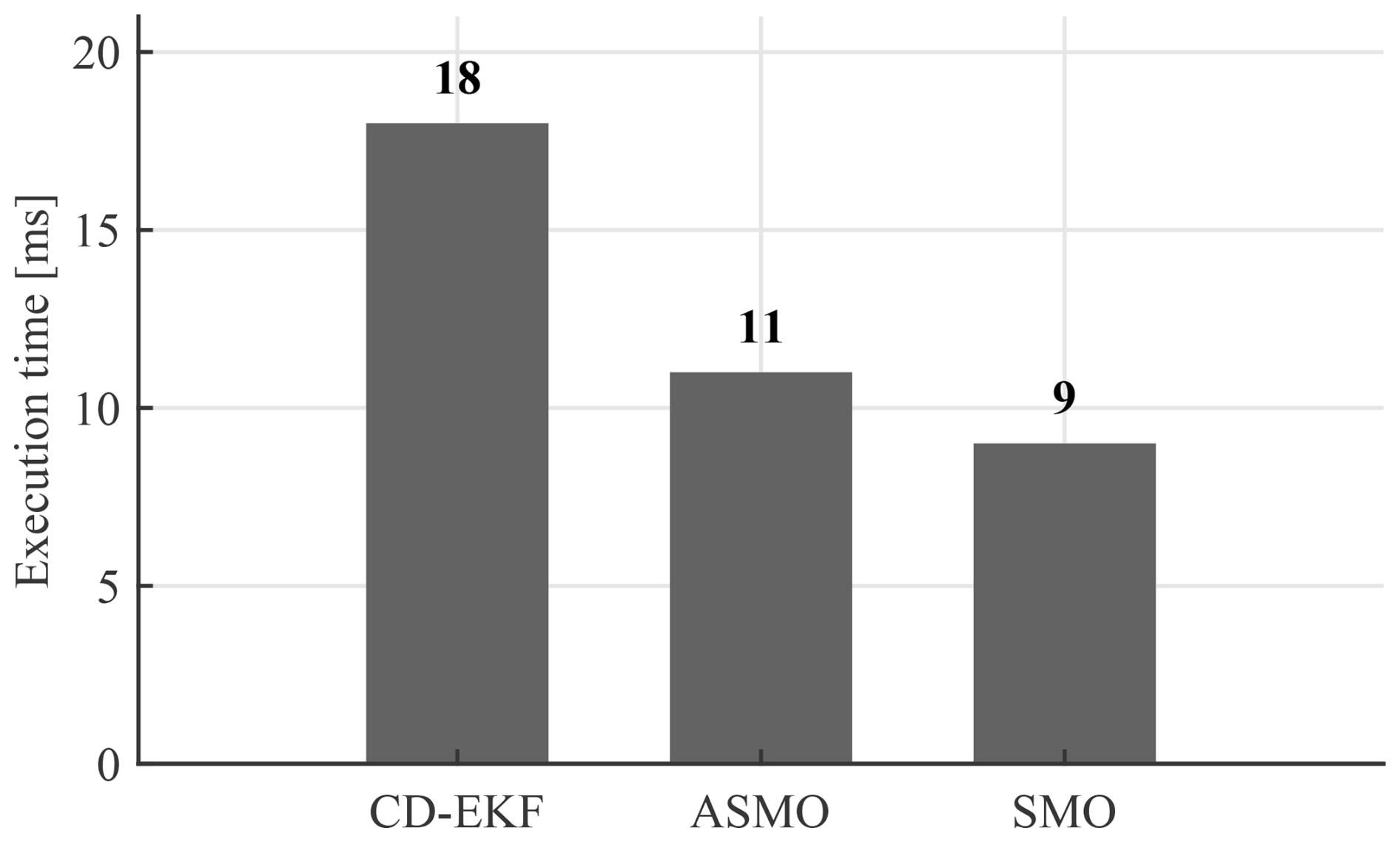
Figure 10 Execution time (in milliseconds) of different observers measured in MATLAB/Simulink Profiler simulations under identical conditions.

5 Experimental results

The proposed observers have been experimentally validated on a SIL setup at École Centrale Nantes, France. The experimental platform consists of a $\mathrm{1}/\mathrm{32}$-scale semi-submersible FOWT, based on the OC4-DeepCwind concept, deployed in the wave tank of the LHEEA laboratory (LHEEA Laboratory, 2025). The physical model includes the floating platform, tower, and mooring system and is instrumented with motion-tracking markers and load sensors, as shown in Fig. 11. This setup provides realistic hydrodynamic excitation through physical wave generation and platform motion.

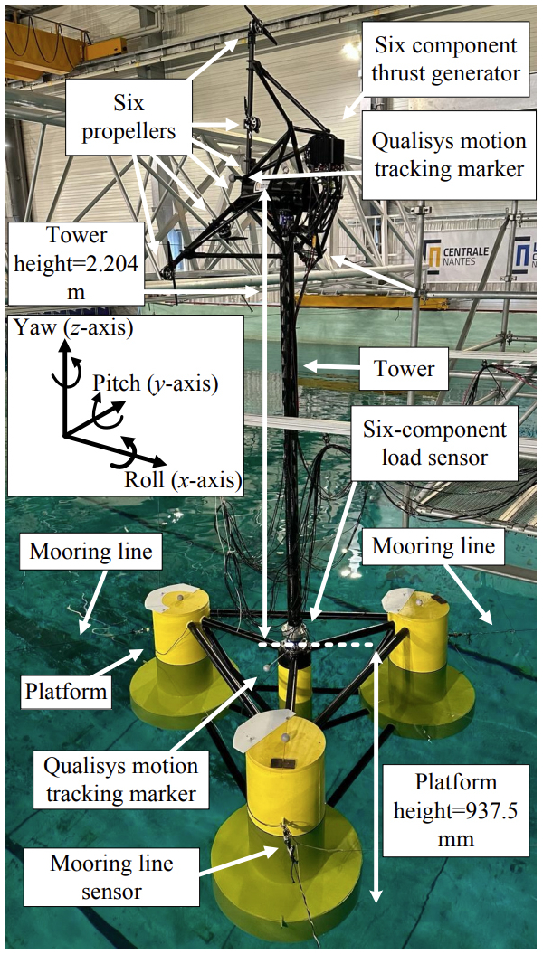
Figure 11 Experimental SIL test setup of the 5 MW $\mathrm{1}/\mathrm{32}$-scale semi-submersible OC4 FOWT at École Centrale Nantes (Aslmostafa et al., 2026).

The overall SIL architecture is illustrated in Fig. 12. In this hybrid configuration, the hydrodynamic processes, wave excitation, viscous and radiation loads, mooring-line forces, and resulting platform dynamics are reproduced physically in the wave tank. Consequently, the corresponding hydrodynamic modules of OpenFAST (HydroDyn, MAP++, MoorDyn or FEAMooring, ElastoDyn), highlighted in the blue dashed region of Fig. 12, are disabled in the numerical simulation. Instead, the measured 6 degrees of freedom platform and tower-top motions from the Qualisys system are imposed as inputs to the real-time numerical model (Bonnefoy et al., 2024). It should be noted that aerodynamic loads are computed numerically. In other words, a modified real-time implementation of OpenFAST runs, where the wind field is prescribed numerically, and the aerodynamic modules (InflowWind, AeroDyn, ServoDyn), highlighted in the red dashed region of Fig. 12, remain active. At each iteration of the SIL loop, the solver receives the measured motions and computes the instantaneous aerodynamic thrust corresponding to the imposed wind field. This thrust is then applied to the physical model by a tower-top actuator system (Fig. 11), enabling consistent aero-hydro coupling during the experiment.

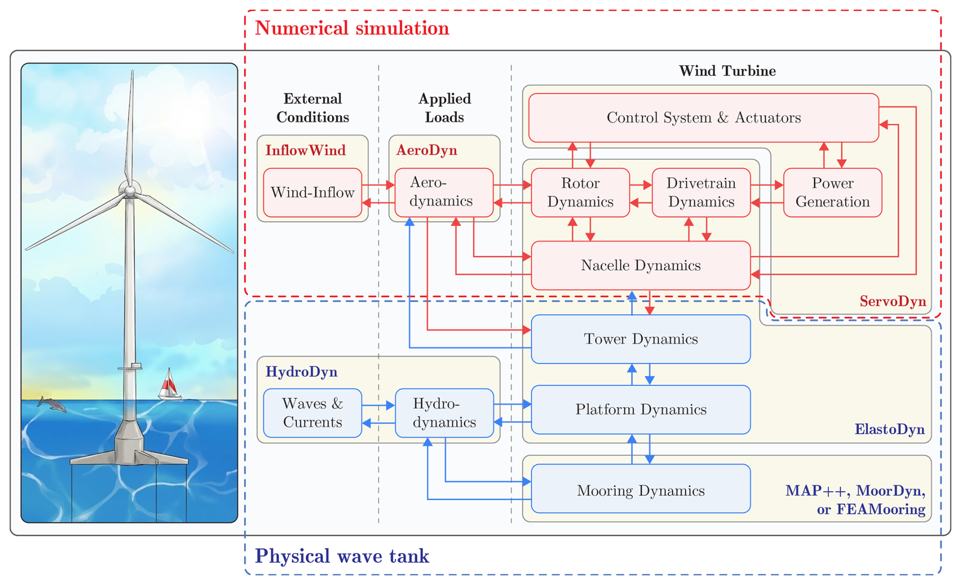
Figure 12 Schematic of the modules in the SIL architecture. The figure is inspired by Bonnefoy et al. (2024) and National Renewable Energy Laboratory (2023). The hydrodynamic and structural modules (blue dashed region) are disabled, as the corresponding processes are reproduced physically in the wave tank, while the aerodynamic modules (red dashed region) remain active and compute real-time aerodynamic loads using the prescribed wind field and measured platform motions.

In the SIL setup, the inflow wind field is numerically prescribed in OpenFAST. Based on this inflow and the instantaneous platform and rotor conditions, OpenFAST computes the corresponding REWS v_r(t), which is used as the reference signal for evaluating the estimation error.

Table 3 outlines selected technical characteristics of both the numerical emulator (OpenFAST) and the scaled experimental setup implemented in the laboratory. The table highlights key parameters of the reference full-scale FOWT alongside those used in the physical test environment.

Table 3 Key specifications of the experimental setup, including both full-scale and corresponding $\mathrm{1}/\mathrm{32}$-scale parameters.

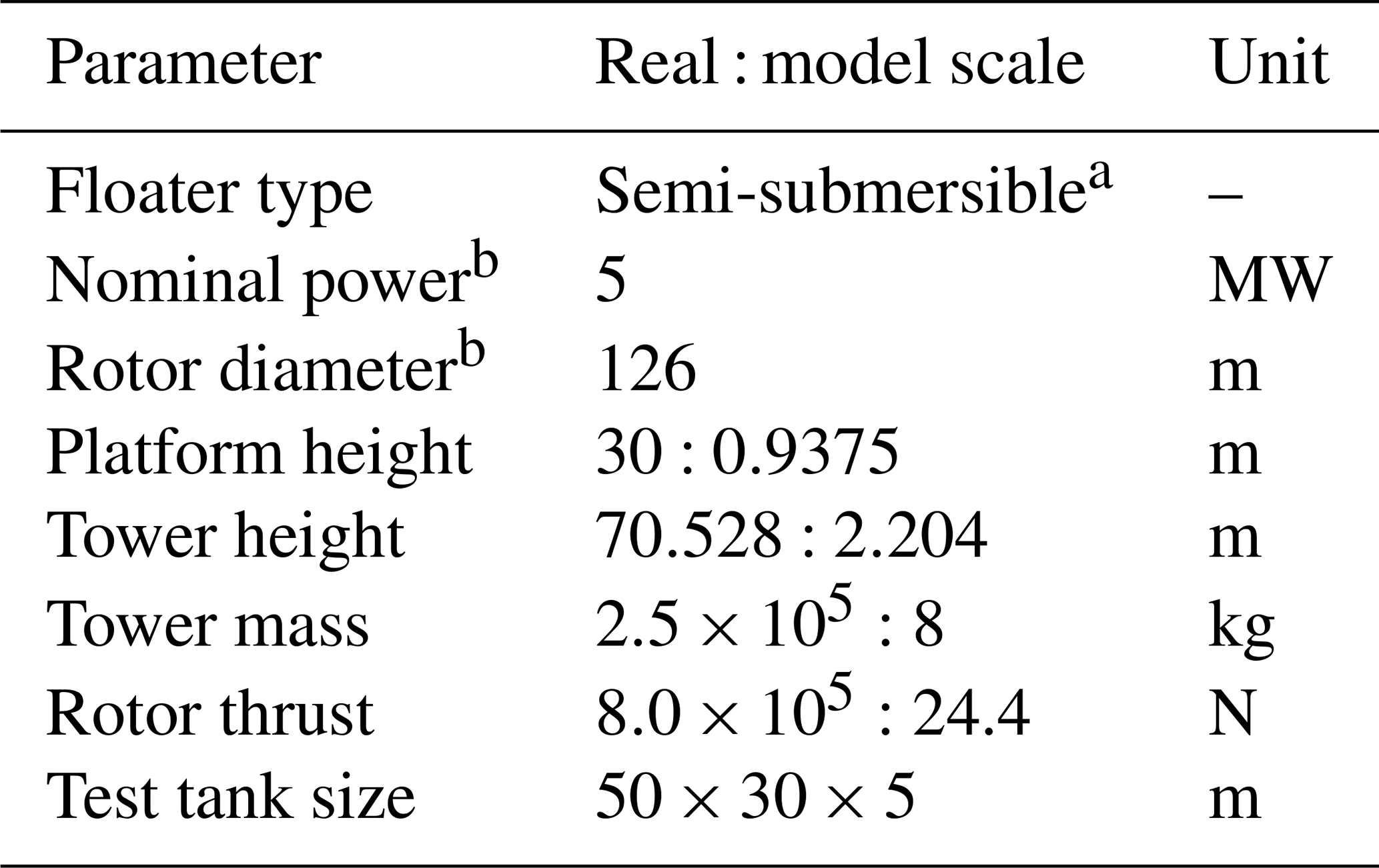
^a Based on the OC4-DeepCwind platform under IEA Wind Task 30 (Robertson et al., 2014). ^b Emulated via software in the loop (SIL).

5.1 Test conditions and scenarios

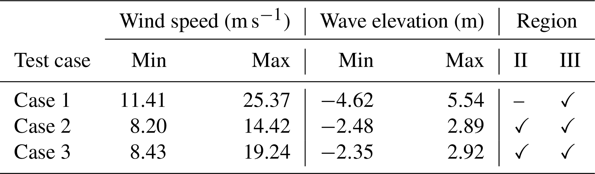
Three test scenarios have been conducted to evaluate the performance and robustness of the proposed observers under various wind and wave conditions, as reported in Table 4. The three datasets were selected under complementary operating regimes as the following:

• Case 1 (Region III only). With $v_{\mathrm{r}}\in [\mathrm{11.41},\mathrm{25.37}]$ m s⁻¹, the turbine operates fully above rated only, highlighting estimator behavior under above-rated operation and strong pitch activity.

• Case 2 (Transition Region II↔III). With $v_{\mathrm{r}}\in [\mathrm{8.20},\mathrm{14.42}]$ m s⁻¹, it covers the transition region, testing robustness to region switching.

• Case 3 (Region II/III). With $v_{\mathrm{r}}\in [\mathrm{8.43},\mathrm{19.24}]$ m s⁻¹, it serves as a general verification across variable conditions from low wind speed to high wind speed.

The three cases collectively address various conditions to ensure a balanced comparison of CD–EKF, SOSMO, and ASOSMO against the actual wind speed.

Table 4 Test conditions for experimental validation, including wind and wave ranges and region classification based on turbine operating regimes.

5.2 Results and discussion

Figures 13–15 illustrate the experimental results for the three test cases. In all scenarios, observers are able to estimate the wind speed despite the presence of wave-induced platform motions and unmodeled dynamics.

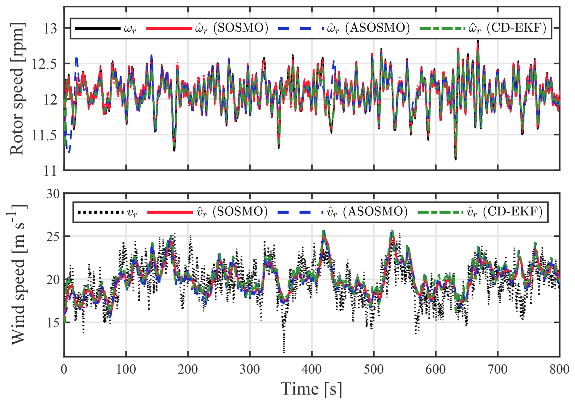
Figure 13 Experimental results for case 1: rotor speed ω_r, REWS v_r, and their estimated values under turbulent wind and wave conditions.

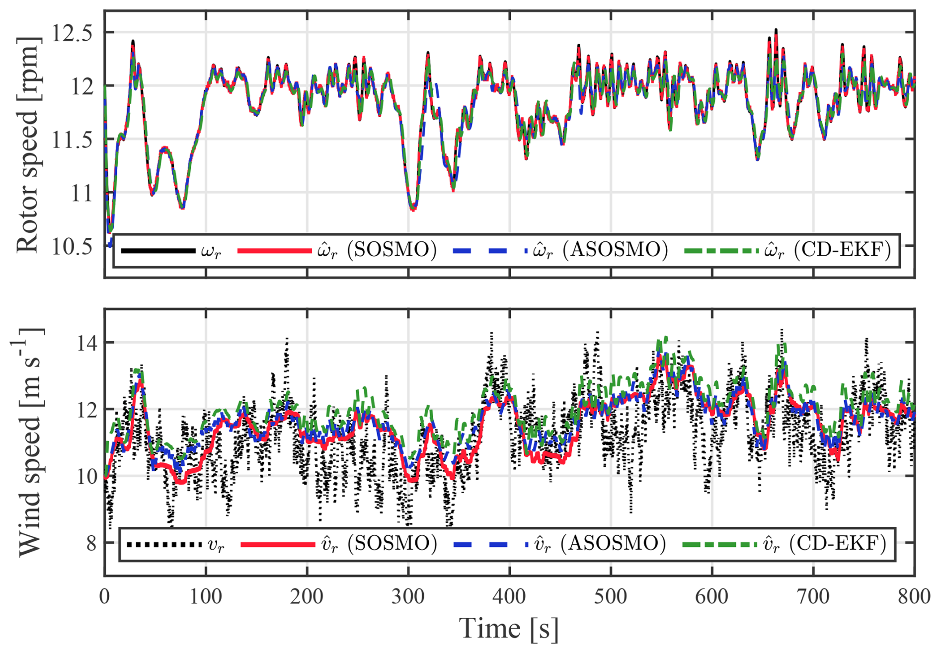
Figure 14 Experimental results for case 2: rotor speed ω_r, REWS v_r, and their estimated values under turbulent wind and wave conditions.

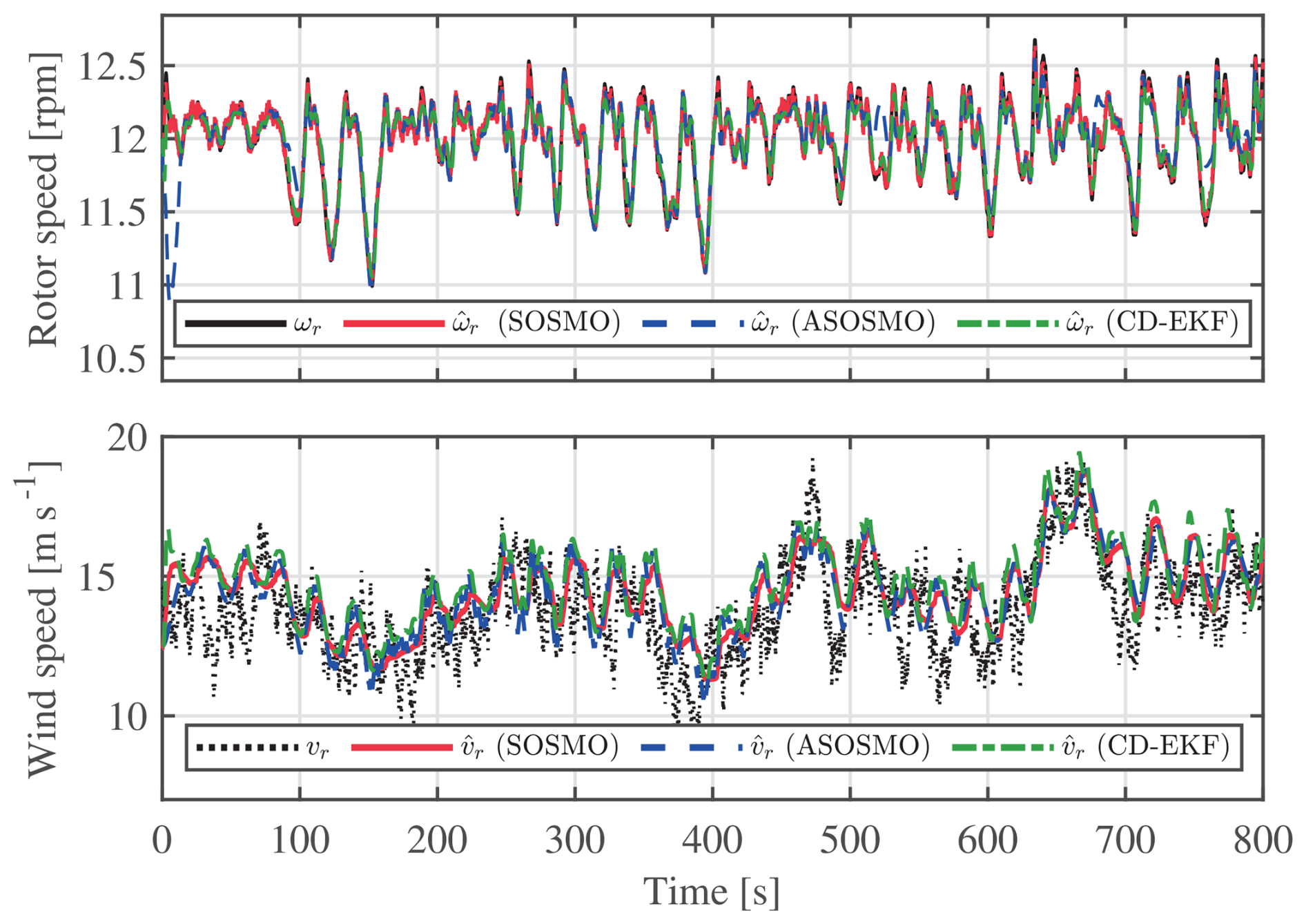
Figure 15 Experimental results for case 3: rotor speed ω_r, REWS v_r, and their estimated values under turbulent wind and wave conditions.

To provide a comprehensive assessment of estimation performance, multiple complementary metrics are considered in both the time and the frequency domains. Let x(k) denote a scalar component of the state vector, namely either the rotor speed ω_r(k) or the REWS v_r(k), $\widehat{x}\left(k\right)$ its estimate, and $e\left(k\right)=\widehat{x}\left(k\right)-x\left(k\right)$ the corresponding estimation error at sample $k=\mathrm{1},\mathrm{\dots },N$. The following statistical indicators are used in this section: (i) the root mean square error $\mathrm{RMSE}=\sqrt{\frac{\mathrm{1}}{N}{\sum }_{k=\mathrm{1}}^{N}e(k{)}^{\mathrm{2}}}$; (ii) the mean estimation error (bias) ${\mathit{\mu }}_{\mathrm{e}}=\frac{\mathrm{1}}{N}{\sum }_{k=\mathrm{1}}^{N}e\left(k\right)$; (iii) the variance of the estimation error ${\mathit{\sigma }}_{\mathrm{e}}^{\mathrm{2}}=\frac{\mathrm{1}}{N-\mathrm{1}}{\sum }_{k=\mathrm{1}}^N\left(e\right(k)-{\mathit{\mu }}_{\mathrm{e}}{)}^{\mathrm{2}}$; and (iv) the mean square error (MSE), defined as $\mathrm{MSE}=\mathbb{E}\left[e^{\mathrm{2}}\right]={\mathit{\sigma }}_{\mathrm{e}}^{\mathrm{2}}+{\mathit{\mu }}_{\mathrm{e}}^{\mathrm{2}}$. Together, these metrics quantify overall accuracy, systematic bias, stochastic dispersion, and the combined effect of bias and variance, as summarized in Table 5.

Table 5 Time-domain statistical performance metrics for CD–EKF, SOSMO, and ASOSMO across three experimental test cases, evaluated for rotor speed ω_r and REWS v_r.

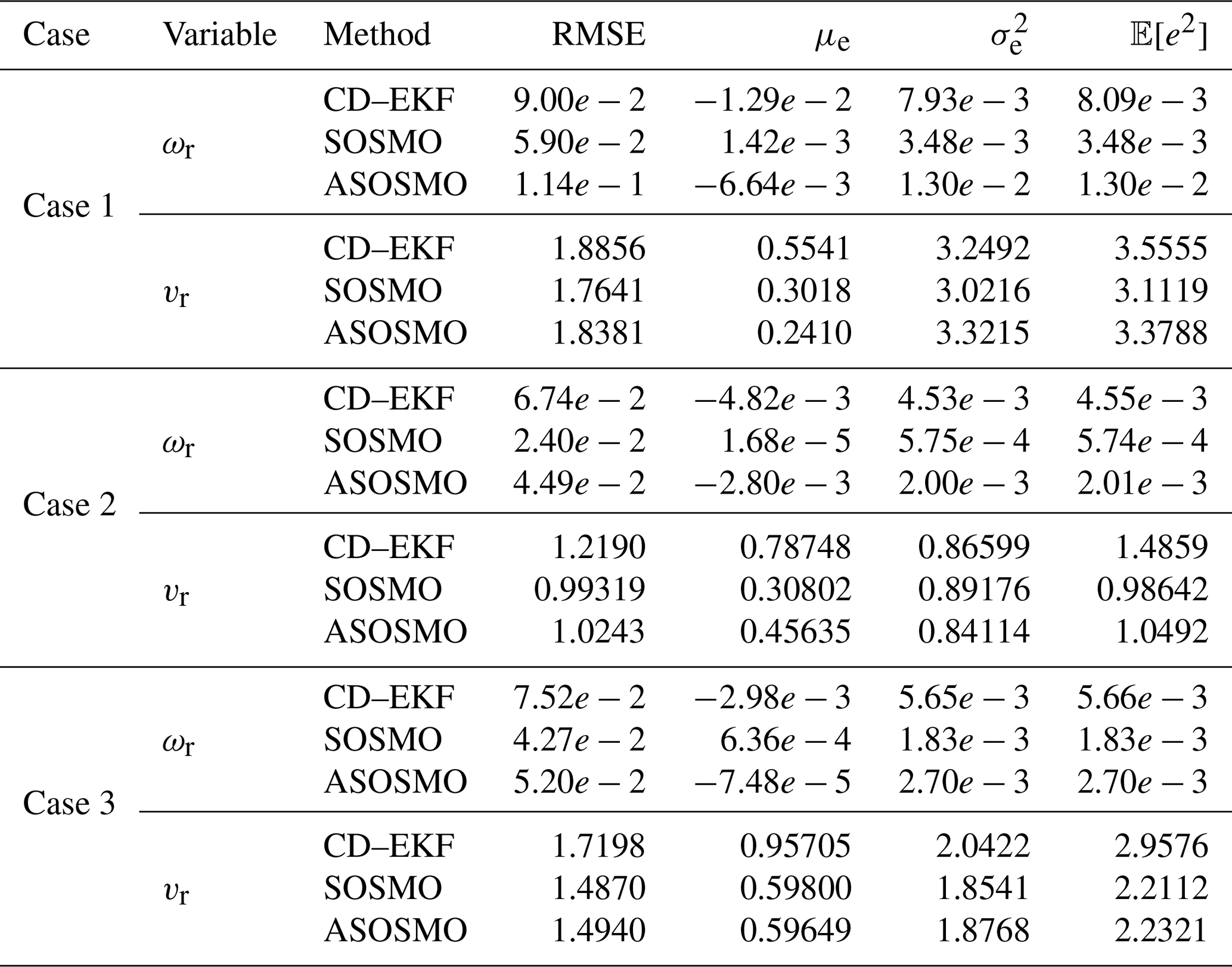
Table 5 shows that all three observers achieve comparable levels of accuracy across the different operating regimes, with variations depending on the wind region and excitation level. In several cases, the sliding-mode observers exhibit reduced bias or variance, while in others the CD–EKF provides similar or slightly lower dispersion. These results indicate that the proposed observers achieve performance levels on par with the reference CD–EKF while relying on fundamentally different estimation principles.

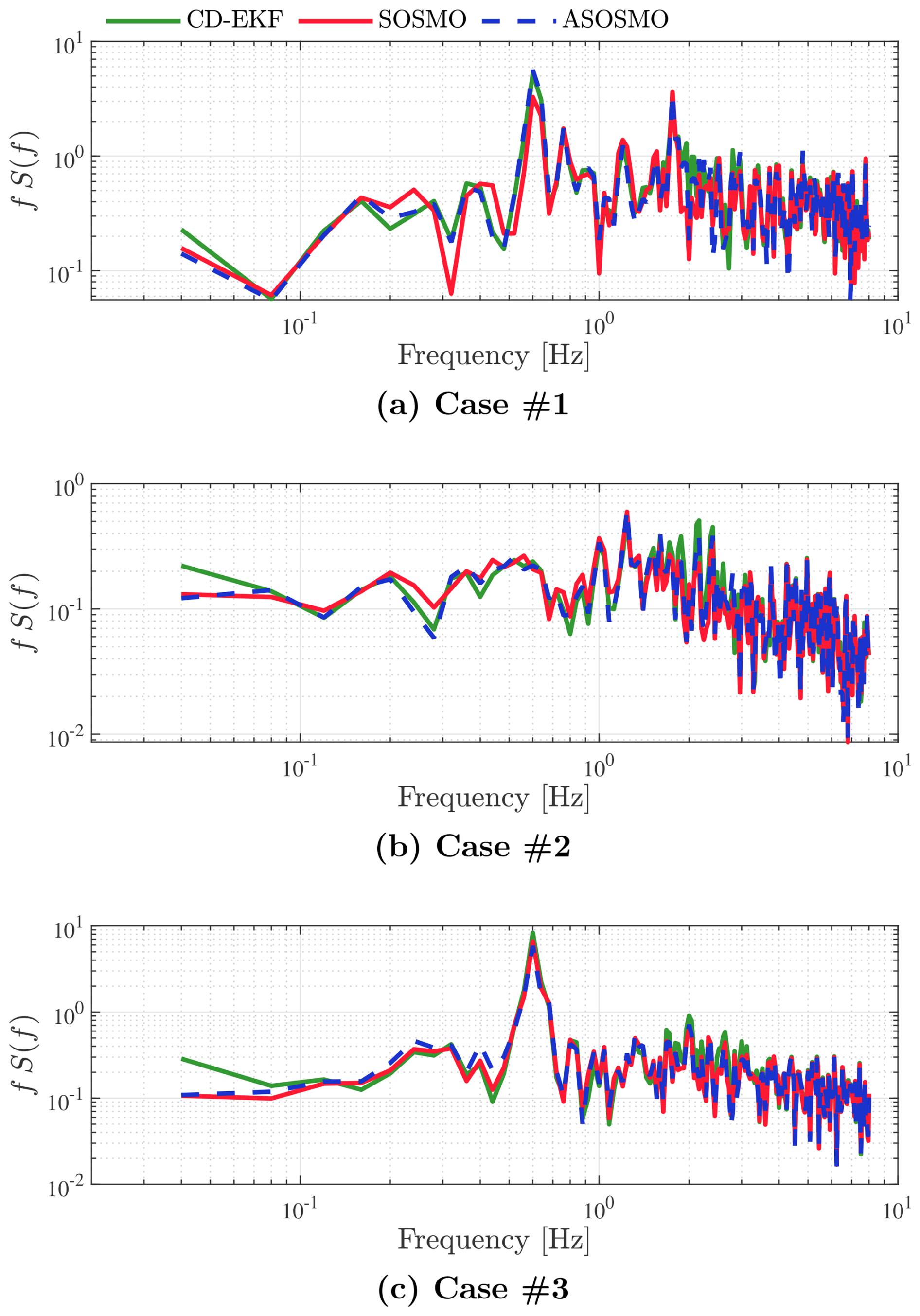
The frequency-domain characteristics of the estimation error are examined through the power spectral density (PSD), shown in Fig. 16. The (one-sided) PSD of the estimation error, denoted by S_e(f), describes how the error energy is distributed across frequencies and is formally defined as

$$\begin{array}{}\text{(35)}& S_{\mathrm{e}}\left(f\right)=\underset{T\to \mathrm{\infty }}{lim}{\displaystyle \frac{\mathrm{1}}{T}}{\left|\underset{\mathrm{0}}{\overset{T}{\int }}e\left(t\right)e^{-j\mathrm{2}\mathit{\pi }ft}dt\right|}^{\mathrm{2}},\end{array}$$

where f denotes frequency. For real-valued signals, a one-sided representation is used so that all spectral energy is contained on the nonnegative frequency axis. In practice, S_e(f) is estimated from the sampled error sequence e(k) using Welch’s method, as implemented in MATLAB via the pwelch function. Following Soltani et al. (2013), the frequency-weighted PSD f⋅S_e(f) is reported to emphasize the contribution of different frequency bands to the overall estimation error.

For all three cases, the three estimators exhibit a similar low-pass behavior, with small differences primarily in the low- and mid-frequency ranges. Depending on the operating condition, the sliding-mode observers and the CD–EKF alternately show lower error energy in specific frequency bands, indicating that none of the approaches systematically dominates across the entire spectrum. Importantly, all estimators preserve a significant portion of the low-frequency content relevant for wind turbine control.

Figure 16 Power spectral density (PSD) of the REWS estimation error in three test cases.

The probabilistic structure of the estimation error is further analyzed through empirical probability density functions (PDFs) (shown in Fig. 17), Specifically, the empirical distribution of the estimation error e(k) is evaluated using a normalized histogram and compared with a Gaussian probability density function parameterized by the sample mean μ_e and variance ${\mathit{\sigma }}_{\mathrm{e}}^{\mathrm{2}}$, given by

$$\begin{array}{}\text{(36)}& p_{\mathrm{Gauss}}\left(e\right)={\displaystyle \frac{\mathrm{1}}{\sqrt{\mathrm{2}\mathit{\pi }}{\mathit{\sigma }}_{\mathrm{e}}}}\exp \left(-{\displaystyle \frac{(e-{\mathit{\mu }}_{\mathrm{e}}{)}^{\mathrm{2}}}{\mathrm{2}{\mathit{\sigma }}_{\mathrm{e}}^{\mathrm{2}}}}\right).\end{array}$$

In all cases, the error distributions are approximately symmetric and well-approximated by Gaussian fits. Differences between observers mainly appear in the spread and centering of the distributions, consistent with the bias and variance values reported in Table 5.

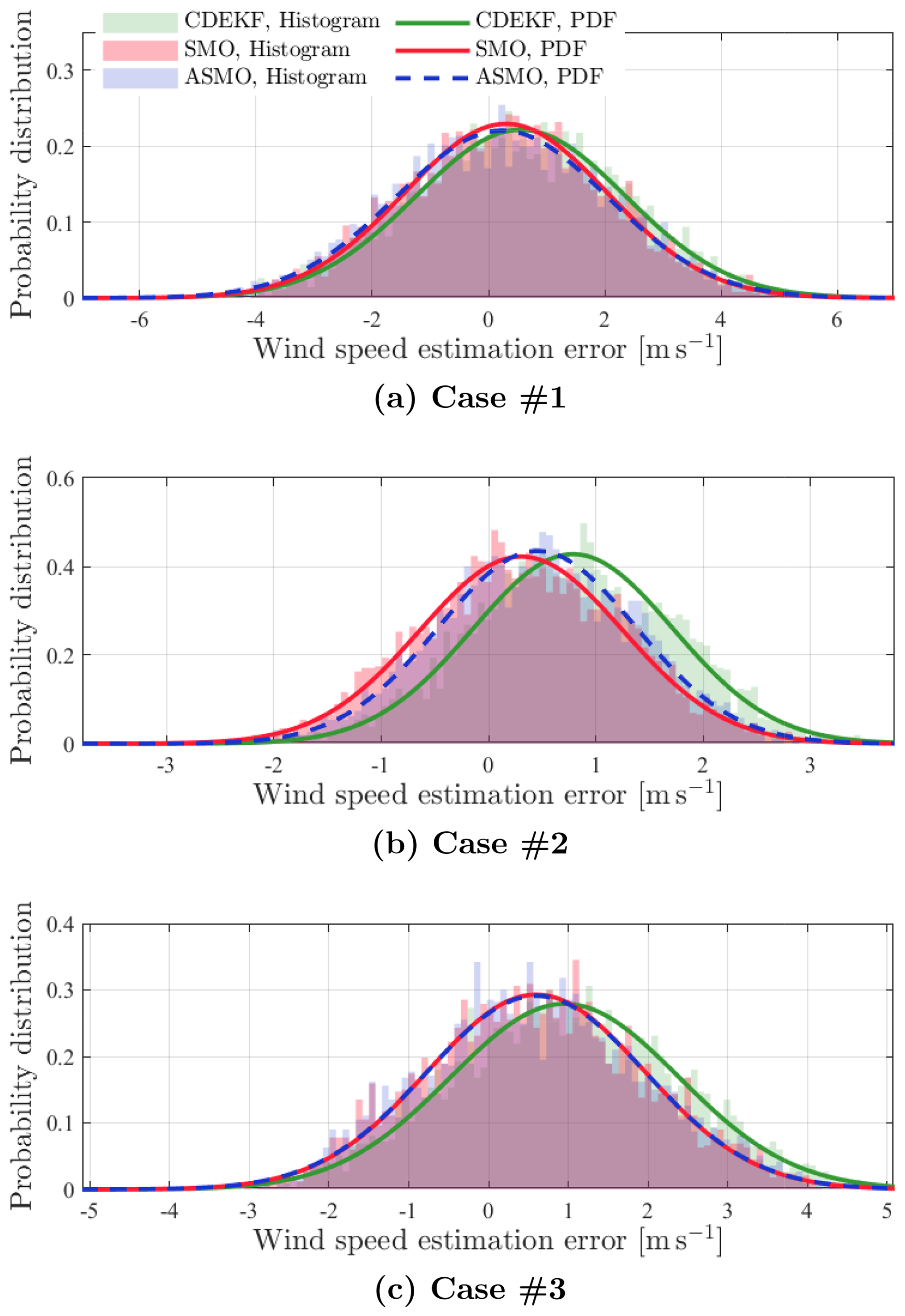
Figure 17 Comparison of the distribution and probability density function (PDF) of the REWS estimation error in three test cases.

Finally, Fig. 18 summarizes the normalized wind speed error metrics for the three observers across the three test cases. The radar representation provides a compact overview of performance trade-offs across RMSE, mean error, variance, and MSE. The results illustrate that the observers exhibit comparable overall performance, with each method showing relative strengths depending on the operating regime and metric considered.

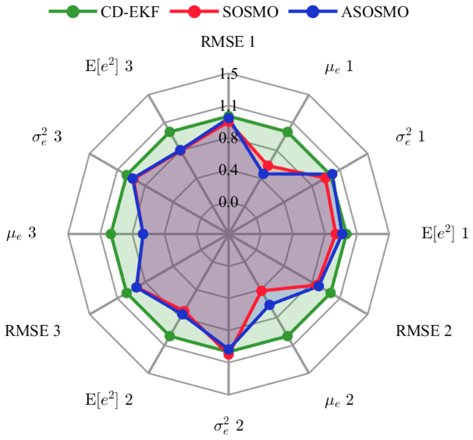
Figure 18 Comparison of normalized error metrics for the three REWS estimation methods: CD–EKF, SOSMO, and ASOSMO, evaluated over three representative wind cases. All metrics are normalized with respect to the CD–EKF baseline.

Overall, the experimental results demonstrate that the proposed second-order sliding-mode observers achieve estimation performance comparable to that of the widely used CD–EKF while offering alternative robustness and tuning characteristics. The multi-metric analysis highlights that no single estimator uniformly outperforms the others across all conditions but rather that each approach provides a viable and reliable solution for REWS estimation in FOWTs under realistic experimental conditions.

6 Conclusions

This paper proposed robust REWS estimation methods based on a second-order sliding-mode observer: a constant-gain second-order sliding-mode observer (SOSMO) and its adaptive version (ASOSMO). The estimation framework is built on a reduced-order nonlinear model and is evaluated not only on the OpenFAST simulator but also through experimental tests where all degrees of freedom are activated.

The two observers are evaluated against the standard continuous–discrete extended Kalman filter (CD–EKF), and they demonstrate accurate tracking of wind dynamics. Unlike CD–EKF, the SOSMO-based methods not only eliminate the need for tuning noise covariance matrices but also avoid the linearization of system dynamics, thereby reducing implementation complexity and improving reliability under modeling uncertainties. Moreover, the adaptive version allows for very limited knowledge of the model.

To summarize, the proposed observers provide a simple yet effective solution for accurate REWS estimation and can be integrated into advanced control strategies. This integration promises improved system stability and reduced fatigue loads when used within appropriate control schemes (e.g., pitch and/or torque control), contributing to the performance of FOWTs. These results mark an initial step toward a comprehensive robust estimation and control framework.

As future work, a fully integrated adaptive-observer-based controller scheme will be developed to further improve the overall performance and resilience of FOWTs.

Appendix A: Continuous–discrete extended Kalman filter

The nonlinear state-space form of a FOWT can be written as

$$\begin{array}{}\text{(A1)}& {\displaystyle }\begin{array}{rl}\dot{\mathit{x}}& =\mathit{f}(\mathit{x},\mathit{u})+\mathit{w}\left(t\right),\\ y_k& =h({\mathit{x}}_k,{\mathit{u}}_k)+v_k,\end{array}\end{array}$$

where $\mathit{x}=[{\mathit{\omega }}_{\mathrm{r}}{v}_t{v}_{\mathrm{m}}{]}^{\top }$ is the state vector, v_t and v_m denote the turbulent and mean wind speed components respectively, and the control input is $\mathit{u}=[{\mathit{\tau }}_{\mathrm{g}}\mathit{\beta }{]}^{\top }$. Additionally, w(t) and v_k are continuous-time and discrete-time white noise, respectively, defined as

$$\begin{array}{}\text{(A2)}& {\displaystyle }\begin{array}{rl}\mathit{w}\left(t\right)& \sim \mathcal{N}(\mathbf{0},\mathbf{Q}),\\ v_k& \sim \mathcal{N}(\mathrm{0},R_{\mathrm{m}}),\end{array}\end{array}$$

where Q is the process-noise covariance matrix, and R_m is the measurement-noise covariance (scalar in this case).

The extended Kalman filter for a continuous–discrete nonlinear system generally consists of two main steps: (i) time update (prediction) and (ii) measurement update (correction), as described in Abbas et al. (2022); Knudsen et al. (2011) as follows:

• Step 1: time update.

  $$\begin{array}{ll}\text{(A3)}& {\displaystyle }{\widehat{\mathit{x}}}_{\mathrm{0}}^{+}& {\displaystyle }=\mathbb{E}\left({\mathit{x}}_{\mathrm{0}}\right)\text{(A4)}& {\displaystyle }{\mathbf{P}}_{\mathrm{0}}^{+}& {\displaystyle }=\mathbb{E}\left[({\mathit{x}}_{\mathrm{0}}-{\widehat{\mathit{x}}}_{\mathrm{0}})({\mathit{x}}_{\mathrm{0}}-{\widehat{\mathit{x}}}_{\mathrm{0}}{)}^{\top }\right]\text{(A5)}& {\displaystyle }\dot{\widehat{\mathit{x}}}\left(t\right)& {\displaystyle }=\mathit{f}\left({\widehat{\mathit{x}}}_{k-\mathrm{1}|k-\mathrm{1}},{\mathit{u}}_k\right){\displaystyle }\dot{\mathbf{P}}\left(t\right)& {\displaystyle }=\mathbf{F}\left(t\right){\mathbf{P}}_{k|k-\mathrm{1}}+{\mathbf{P}}_{k|k-\mathrm{1}}{\mathbf{F}}^{\top }\left(t\right)+\mathbf{Q}\\ \text{(A6)}& {\displaystyle }& {\displaystyle }-{\mathbf{K}}_{k-\mathrm{1}}{R}_{\mathrm{m}}{\mathbf{K}}_{k-\mathrm{1}}^{\top }\end{array}$$

  Here $\mathbf{F}\left(t\right)={\left.\frac{\partial \mathit{f}}{\partial \mathit{x}}\right|}_{{\widehat{\mathit{x}}}_{k-\mathrm{1}|k-\mathrm{1}},{\mathit{u}}_k}$ is the Jacobian matrix of the nonlinear dynamics, and P is the estimation-error covariance. The estimate ${\widehat{\mathit{x}}}^{+}$ represents the state updated using y_k, while ${\widehat{\mathit{x}}}^{-}$ denotes the prediction using y_k−1.

• Step 2: measurement update.

  $$\begin{array}{}\text{(A7)}& {\displaystyle }{\mathbf{K}}_k& {\displaystyle }={\mathbf{P}}_{k|k-\mathrm{1}}{\mathbf{H}}_k^{\top }{\left({\mathbf{H}}_k{\mathbf{P}}_{k|k-\mathrm{1}}{\mathbf{H}}_k^{\top }+R_{\mathrm{m}}\right)}^{-\mathrm{1}}\text{(A8)}& {\displaystyle }{\widehat{\mathit{x}}}_{k|k}& {\displaystyle }={\widehat{\mathit{x}}}_{k|k-\mathrm{1}}+{\mathbf{K}}_k\left(y_k-h\left({\widehat{\mathit{x}}}_{k|k-\mathrm{1}}\right)\right)\text{(A9)}& {\displaystyle }{\mathbf{P}}_{k|k}& {\displaystyle }=(\mathbf{I}-{\mathbf{K}}_k{\mathbf{H}}_k){\mathbf{P}}_{k|k-\mathrm{1}}\end{array}$$

  Here ${\mathbf{H}}_k={\left.\frac{\partial h}{\partial \mathit{x}}\right|}_{{\widehat{\mathit{x}}}_{k|k-\mathrm{1}}}$ is the Jacobian matrix of the measurement function, and K_k is the Kalman gain.

  The process-noise covariance is chosen as

  $$\begin{array}{}\text{(A10)}& {\displaystyle }\mathbf{Q}=\mathrm{diag}\left\{\mathrm{1}\times {\mathrm{10}}^{-\mathrm{5}},{\displaystyle \frac{\mathit{\pi }{v}_{\mathrm{m}}^{\mathrm{3}}{t}_i^{\mathrm{2}}}{L}},{\displaystyle \frac{\mathrm{4}}{\mathrm{600}}}\right\},R_{\mathrm{m}}=\mathrm{0.02},\end{array}$$

  and using the relation ${\widehat{v}}_{\mathrm{r}}=v_t+v_{\mathrm{m}}$, the estimation of the REWS is calculated.

Appendix B: Nomenclature

Abbreviations

ASOSMO	Adaptive second-order sliding-mode observer
CD–EKF	Continuous–discrete extended Kalman filter
EKF	Extended Kalman filter
FOWT	Floating offshore wind turbine
KF	Kalman filter
NREL	National Renewable Energy Laboratory
REWS	Rotor-effective wind speed
ROSCO	Reference open-source controller
SIL	Software in the loop
SMO	Sliding-mode observer
SOSMO	Second-order sliding-mode observer
STW	Supertwisting

Symbols and parameters

α,ε	Design parameters of the adaptive law [–]
β	Blade pitch angle [°]
λ	Tip-speed ratio [–]
${\mathit{\omega }}_{\mathrm{r}},{\widehat{\mathit{\omega }}}_{\mathrm{r}}$	Real and estimated rotor speed [rpm]
ρ	Air density [kg m−3]
τa	Aerodynamic torque [N m]
${\mathit{\tau }}_{\mathrm{g}},{\mathit{\tau }}_{\mathrm{g}}^{*}$	Generator torque, rated value [N m]
Cp	Power coefficient (function of λ, β) [–]
J	Total rotational inertia [kg m2]
k1,k2	Adaptive observer gains [–]
ng	Gearbox ratio [–]
Pa	Aerodynamic power extracted by the rotor [W]
Pwind	Theoretical wind power [W]
R	Rotor radius [m]
u	Control input vector
$v_{\mathrm{r}},{\widehat{v}}_{\mathrm{r}}$	True and estimated rotor-effective wind speed [m s−1]
v∞	Free-stream (upstream) inflow wind speed [m s−1]
z	Observer coordinate vector