Trimming a rigid-wing airborne wind system for coordinated circular flights

Airborne wind energy systems (AWESs) are tethered flying devices used for electricity generation. During the power-generation phase, the aerial component usually flies in a circular or figure-of-eight pattern. This paper examines the control surface movements required for circular flights in rigid-wing AWESs. In the absence of gravity, steady trim with equilibrium solutions can be achieved if the orbit plane is normal to the wind. The radius depends on how much the aircraft leans into the turn: leaning in reduces the radius and is statically stable, while leaning out achieves a larger radius but is unstable. For the latter case, artificial stabilisation can be done by cross-feeding the pitch and roll responses to the aileron. For circular trajectories that are not normal to the wind (i.e. experiencing out-of-plane wind), energy needs to be added to the system through the periodic forcing of a control surface. The correct timing of the forcing will excite the orbit's natural frequency, enabling full control of the circle centre and orientation for navigation in the 3D space. This can be done even in the presence of gravity, which is discussed in the second half of this paper. The aileron is the most effective control effector for forcing. Although the trimming method presented in this paper is only suitable for theoretical studies, it provides insights into the flight dynamics of rigid-wing AWESs and lays the groundwork for future flight control developments.

1 Introduction

First formally conceptualised by Loyd (1980), airborne wind energy systems (AWESs) harvest wind energy using a tethered flying device. The main advantage of AWESs is its lightweight construction, which reduces material usage and the lifetime carbon footprint compared to conventional wind turbines of similar outputs. Research into AWESs has grown significantly in the past two decades, with research groups and startups proposing increasingly innovative designs. An overview of AWES technology can be found in Pereira and Sousa (2023).

Since AWESs lack a solid structural foundation seen in conventional wind turbines, the number of degrees of freedom expands from 1 to 6 (excluding structural deformation). Control, therefore, becomes one of the most critical aspects for safe and reliable AWES operations (Vermillion et al., 2021). AWES control is a large topic and can be split into flight control and ground winch control, with the former further split into distinct phases of operation (launch, power generation, retraction, and landing). In this work, we focus on the power-generation phase of groundgen AWESs, which generates energy by converting kinetic energy into traction force on the tether, which is connected to the ground generator. The flight path in the power-generation phase is usually in a figure-of-eight or circular pattern (Eijkelhof et al., 2024). Circular flight is the focus of this paper (see Fig. 1). In this work, we refer to the tethered aerial component as an aircraft instead of a kite to underline the use of traditional control surfaces (aileron, elevator, and rudder).

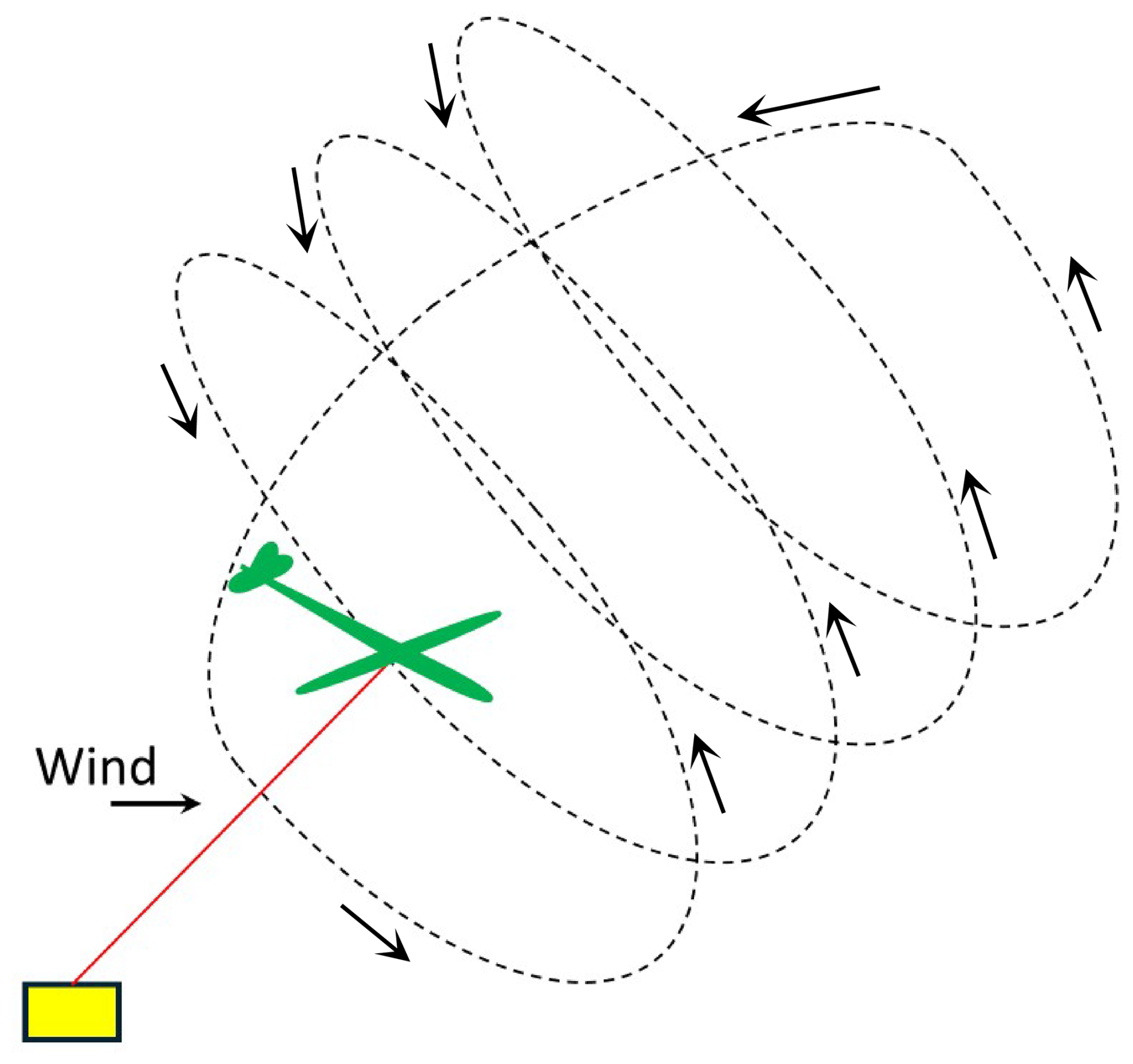
Figure 1 Schematic of a full power production cycle, showing the power-generation phase (flown in circular pattern) followed by retraction. Illustration by Kevin Yu (University of Bristol).

Various flight control strategies for the power-generation phase have been presented, including dynamic inversion combined with cascaded control (Rapp et al., 2019), optimisation-based with frequency-domain characteristics (Trevisi et al., 2022), and “L0 and L1” guidance (Fernandes et al., 2022; Vinha et al., 2025). All these works took a feedback control approach, where the goal is to guide the tethered aircraft along a predefined path. To corroborate the understanding of those AWES control laws, this paper provides an open-loop perspective: determining which control surface movements will put the tethered aircraft in a circular flight path. The discussions will provide an insight into the flight dynamics of rigid-wing AWESs and help to explain how different control algorithms achieve the same physical outcome. Results are fundamental in nature and may not constitute a feasible feedback strategy. However, the idea can be expanded for a future flight control system with a feedforward term.

Prior research focusing on the flight dynamics aspect has successfully analysed AWES flight as a static problem (Trevisi et al., 2021; Rapp, 2021). In this work, we expand the discussion to examine the cyclic nature of AWES flight due to the presence of gravity and out-of-plane wind. It will be shown that AWES circular flight requires periodically exciting one of the three control surfaces at the natural frequency of the cycle, with the aileron being the most effective option. The use of aileron agrees with observations from a prior study, which noted that the simplest control strategy for AWESs is to cyclically actuate the aileron – see Chap. 7 in Trevisi (2024). Our analysis of the cyclic control inputs takes a time-domain-based approach, which provides an alternative perspective to the frequency-domain analysis provided in Trevisi et al. (2022).

The first result section of this paper focuses on static trim in zero gravity, noting the difference in static stability between small and large-radius circular orbits. A method to stabilise the unstable large-radius orbits is then proposed. Subsequently, dynamic trim is introduced to achieve circular flight in the presence of out-of-plane wind and gravity. The dynamic trim method will be shown to be a means of exciting the natural frequency of the circular orbit trajectory, which provides the energy needed to achieve circular flight despite the energy losses from out-of-plane wind and gravity.

2 Simulation model

The analysis was done using a 6-degree-of-freedom simulation of Kitemill's KM1 AWES. The KM1 is a 20 kW groundgen prototype driven by a 54 kg, 7.4 m wingspan aircraft with vertical takeoff and landing capability (see Fig. 2). The simulation contains the states listed in Table 1. Previous studies that have used the same simulation include Mohammed et al. (2024a, b). computational fluid dynamics was used to construct the aerodynamic data. For illustrative purposes, Figs. 3 and 4 present a small set of key aerodynamic relationships as functions of angle of attack and sideslip. The aircraft also has a set of flaps for additional lift during power production, which is set to its maximum deflection of 13° in this paper.

Figure 2 Aerial component of the Kitemill KM1 system.

Table 1 Summary of the states in the simulation.

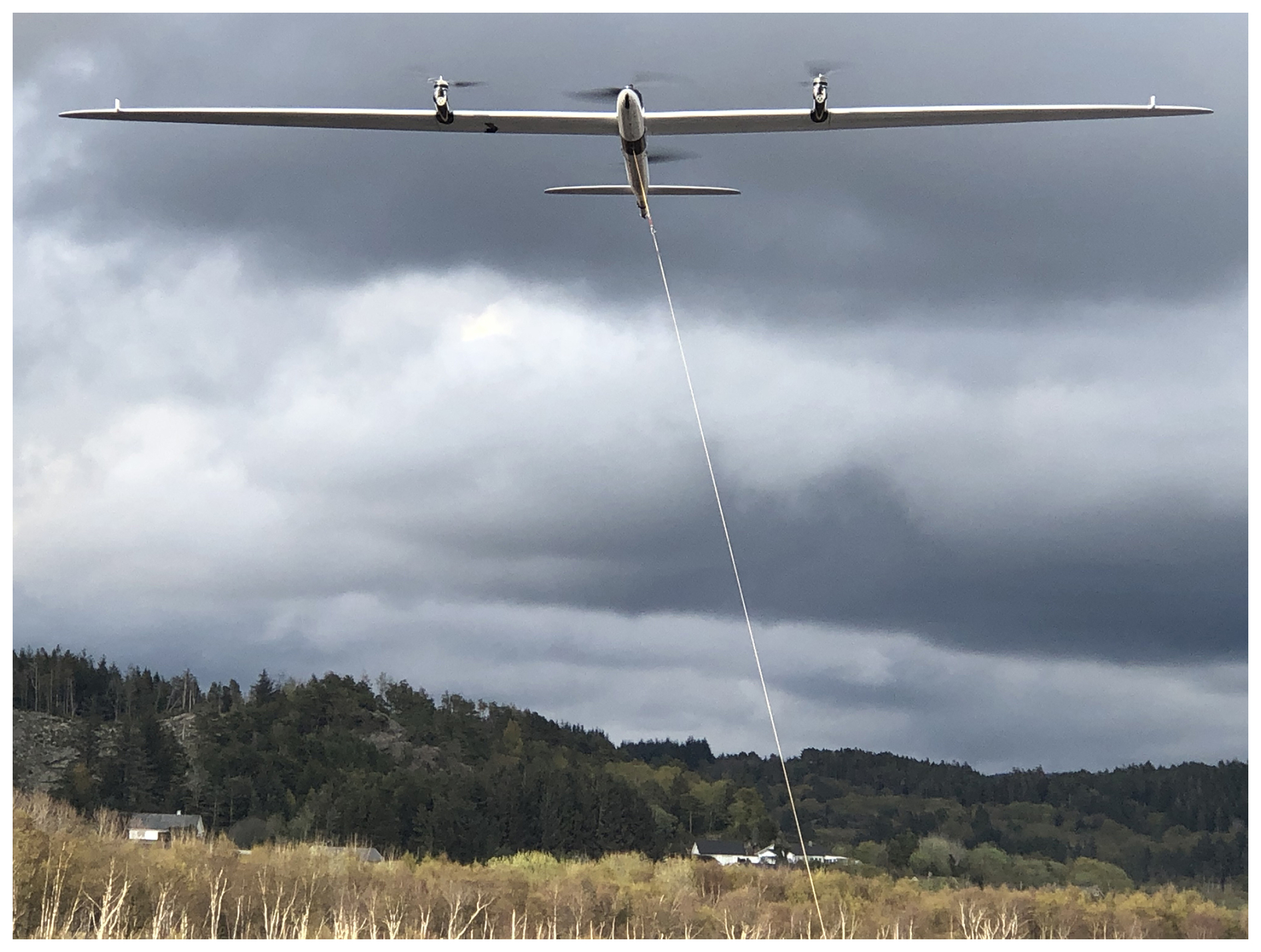
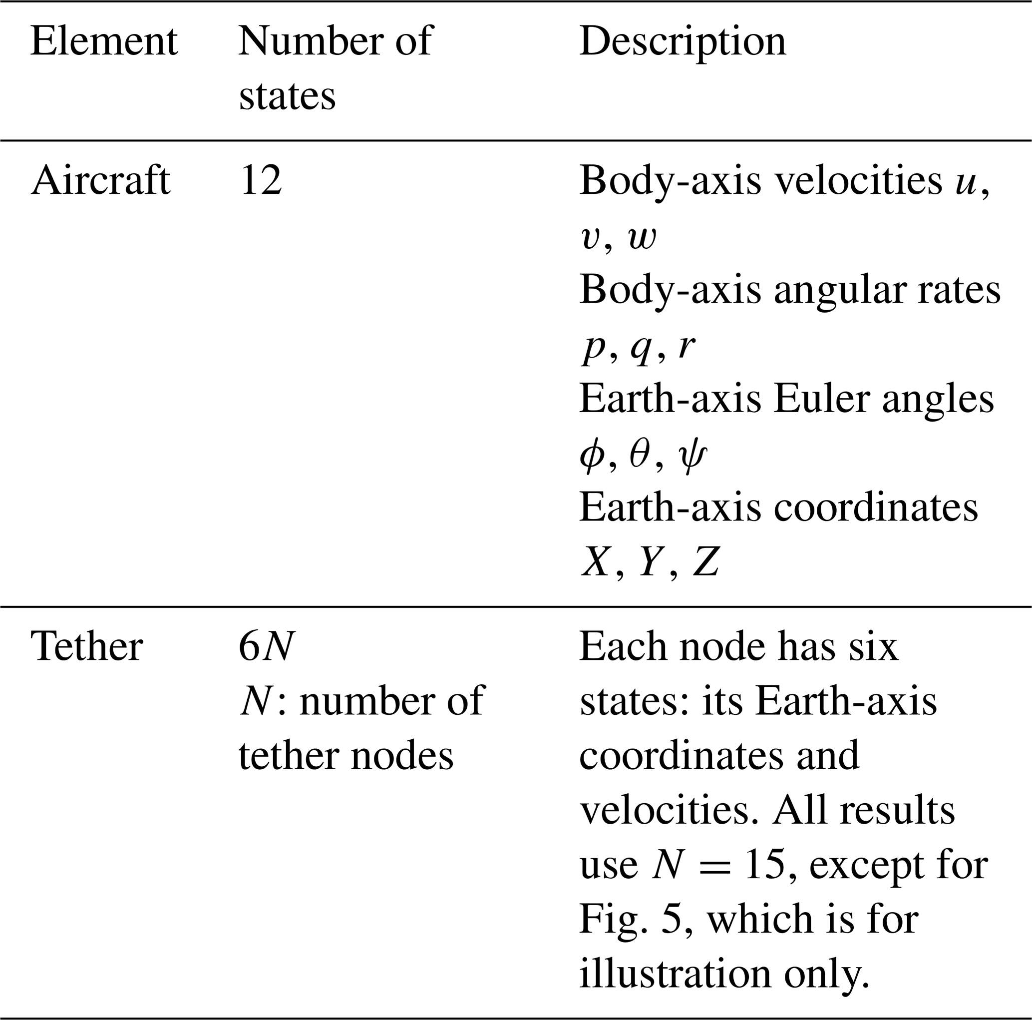
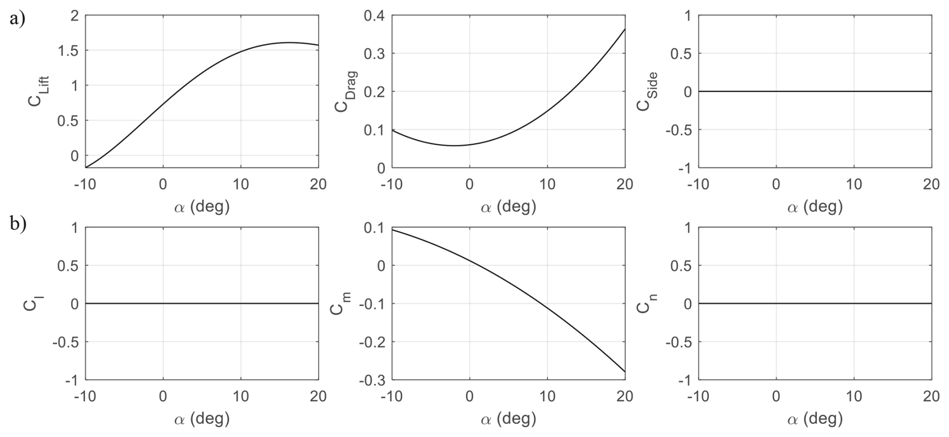
Figure 3 Aerodynamic (a) force and (b) moment coefficients as functions of the angle of attack at zero sideslip, flaps, and control surface deflections.

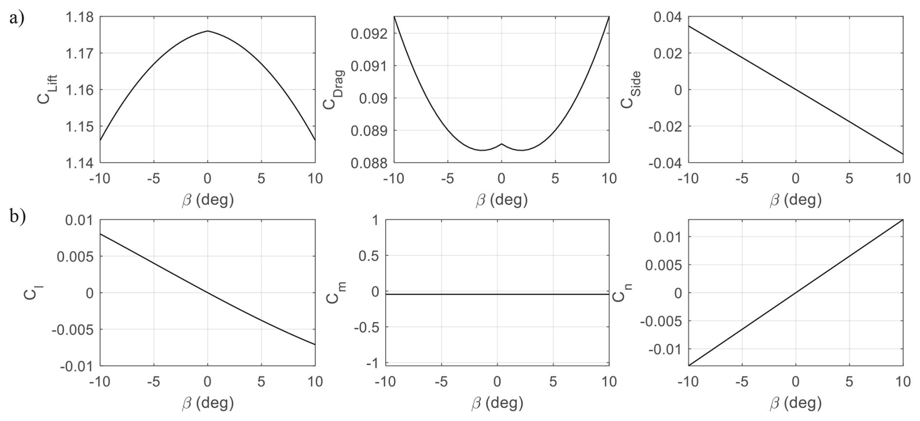
Figure 4 Aerodynamic (a) force and (b) moment coefficients as functions of the sideslip angle at 5° angle of attack, zero flaps, and no control surface deflections.

The tether model accounts for both tether weight and drag, as well as mechanical stiffness and damping between nodes. Each tether segment is a mass-spring-damper system bounded by a node on each end. The nodes are placed along the tether length using cosine spacing, which allocates more nodes towards the aircraft than near the winch (see Fig. 5). This is to reflect the increased tether bending downwind. Compared to linear node spacing, cosine spacing provides similar fidelity for a lower computational cost. Most results presented involve a fixed tether length of 350 m with 15 nodes, thereby omitting the need for modelling a ground winch. A measurement of 350 m was chosen as this is the typical tether length at the start of reel out. The total number of states in this configuration is 102.

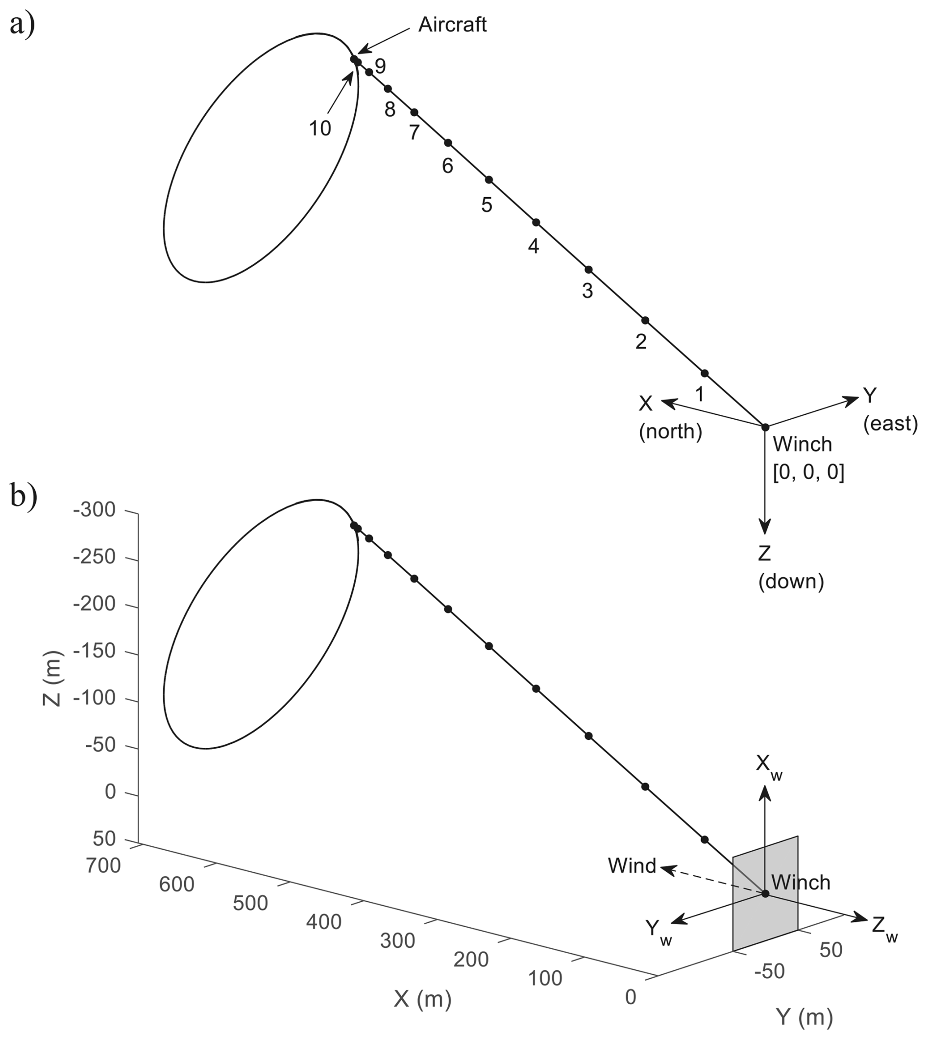
Figure 5 (a) Earth-axis and (b) wind-axis coordinate systems. Both figures show a tether with 10 nodes.

Figure 5 shows the two coordinate systems used. The first one (Fig. 5a) comprises the X, Y, and Z axes, which originate from the ground winch and point in the north, east, and down directions, respectively. X, Y, and Z describe the aircraft's location with respect to the flat Earth, and are used as axis labels in all 3D figures from this point onwards.

A second coordinate system, called the wind frame, is shown in Fig. 5b (not to be confused with the wind axis/body axis distinction in the aerodynamic sense). The wind frame is an inertial frame with its origin fixed at the winch. Its three axes – X_w, Y_w, and Z_w – are oriented such a way that Z_w is opposite the wind direction, resulting in X_w and Y_w forming a plane normal to the wind. From this frame, a second set of Euler angles ϕ_w, θ_w, and ψ_w, relative to the X_w–Y_w plane, can be defined. Note that ψ_w=0° results in the aircraft's nose pointing up, relative to the flat Earth. The purpose of the $[{\mathit{\varphi }}_{\mathrm{w}},{\mathit{\theta }}_{\mathrm{w}},{\mathit{\psi }}_{\mathrm{w}}]$ set is to help visualise the turning motion relative to the wind more intuitively. For example, a left-turning circular trajectory on the wind frame with the wing perfectly perpendicular to the wind should have ϕ_w=0°, θ_w=0°, and ψ_w decreasing. In this work, the wind is assumed to be steady at 10 m s⁻¹ and travels in the positive x direction (south to north).

3 Static trim without gravity

“Static trim” refers to fixing the control surfaces at a constant deflection (as opposed to periodically forcing them, which will be discussed in subsequent sections). In an environment with no gravity and constant tether natural length, an aircraft trimmed for circular flight will converge to an orbit normal to the wind, with the centre at $[Y,Z]=[\mathrm{0},\mathrm{0}]$ (i.e. overlapping the winch on the YZ plane). Figure 6 shows a few such trajectories, where the aircraft (drawn to scale here and in all subsequent figures) has been trimmed for a 6° angle of attack α and zero sideslip β at different radii. The radius R is correlated to the roll angle ϕ_w in the wind frame – henceforth referred to as the lean angle. For left turn cases, as shown, negative ϕ_w means more left roll, i.e. leaning more into the turn.

Figure 6 Circular trajectories without gravity for α=6° and β=0°.

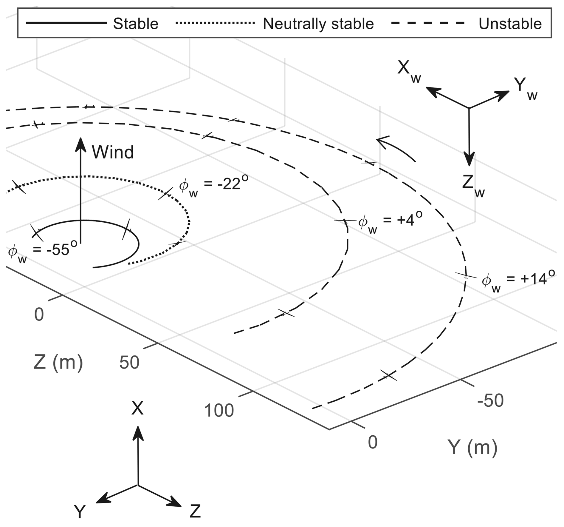
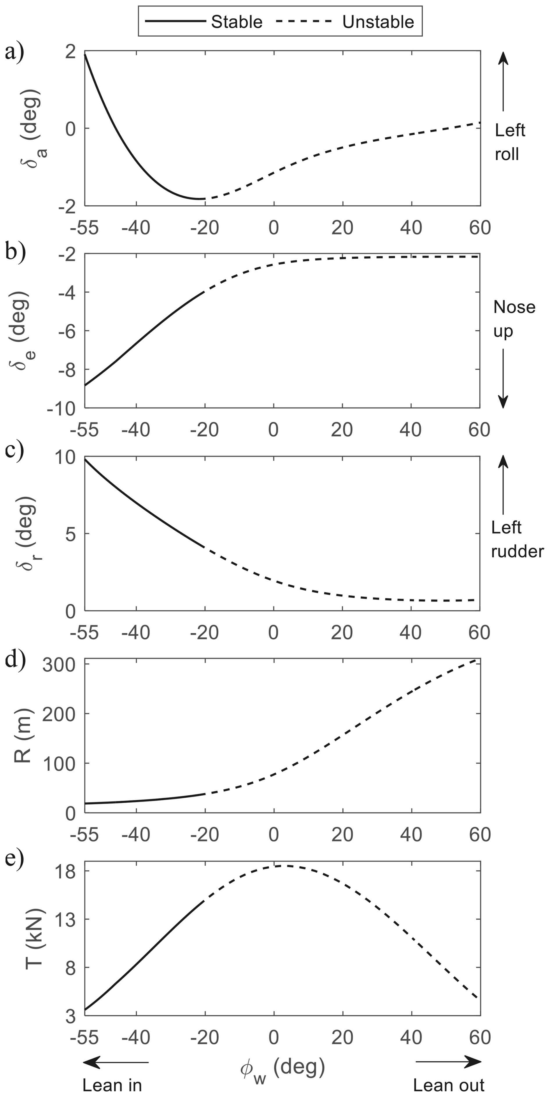
Figure 7 Relationship between lean angle ϕ_w and (a–c) control surface deflections, (d) radius, and (e) tether tension to achieve trimmed flight at α=6° and β=0°. The minimum radius is limited by rudder travel range (10°).

Figure 8 (a) Trajectory and (b) time histories of the lean-out instability at ϕ_w=15°.

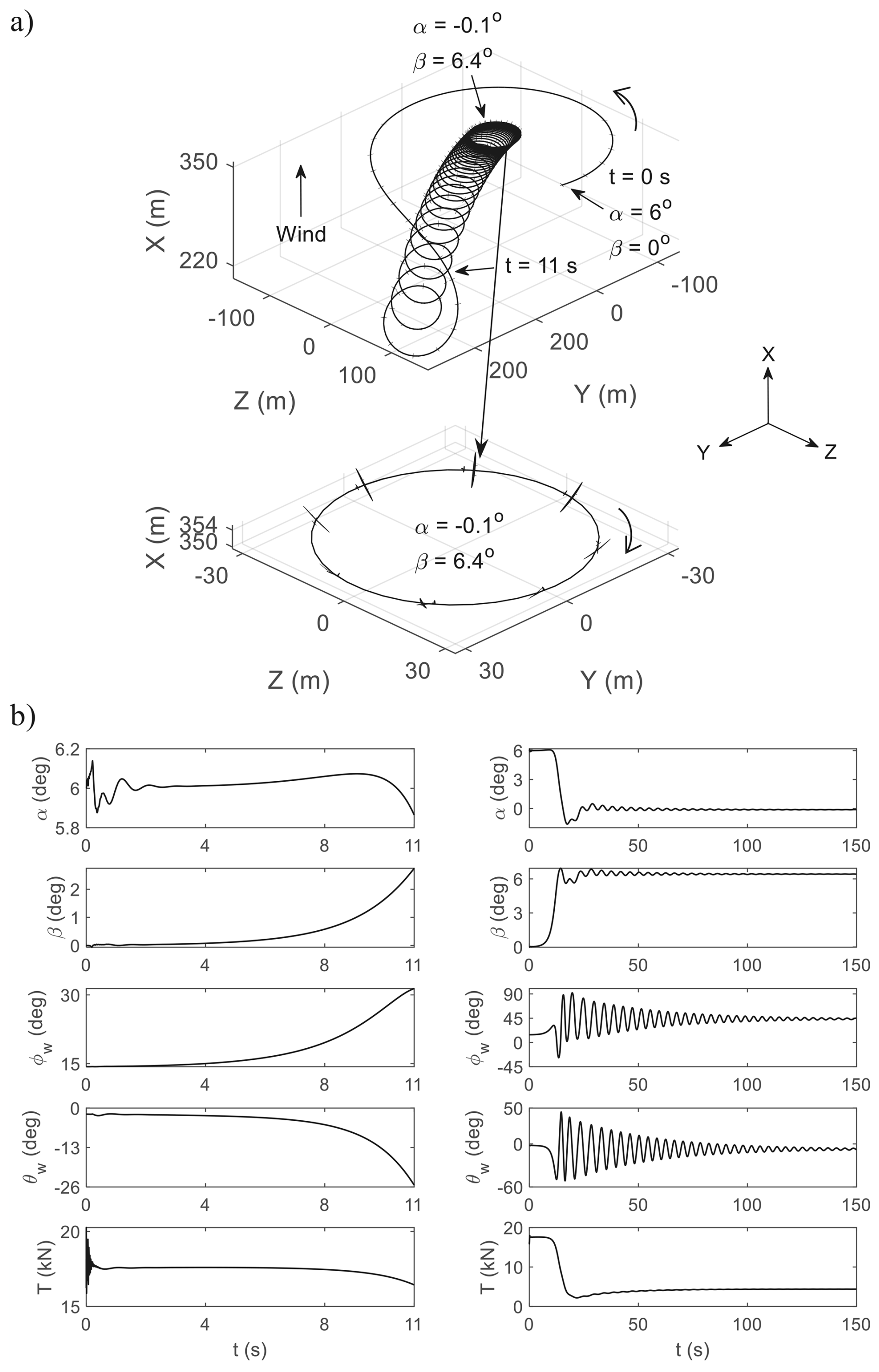
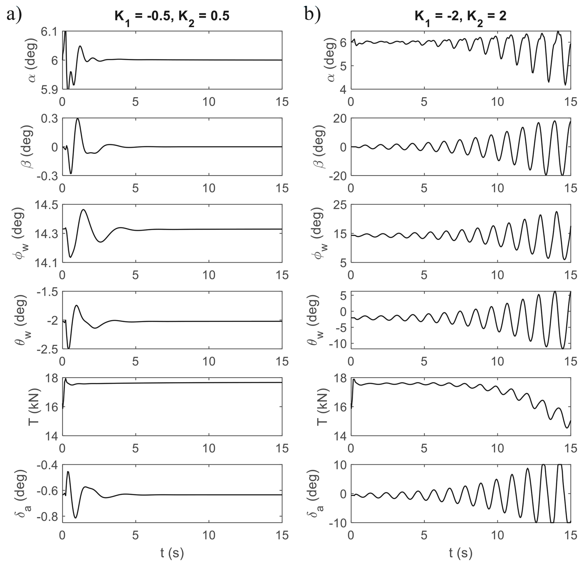
Figure 9 Cross-feeding roll and pitch into aileron to stabilise a 15° lean-out orbit, showing responses to (a) appropriate and (b) excessive gains.

Figure 7 shows the relationship between ϕ_w and radius R, tether tension at the winch T, and control surface deflections (aileron δ_a, elevator δ_e, and rudder δ_r). Trimming and stability were determined using the numerical continuation software AUTO 07-P (Doedel et al., 2021) interfaced in the MATLAB/Simulink environment via the Dynamical Systems Toolbox (Coetzee et al., 2010). Some notable features of Fig. 7 are as follows:

• Rolling is the primary mechanism for changing the radius. In panel (d), leaning more into the turn reduces the radius.

• In panel (e), there is a maximum value for the tether tension at 2.8° lean out. Achieving higher tension is correlated with higher power for energy generation. A potential explanation for the optimal angle being slightly above 0° is that at 0°, the wing is normal to the wind and hence receives the most wind. However, the outer wing travels slightly faster than the inner wing and hence generates more lift. A few additional degrees of leaning out equalise the lift on both wings for optimal power generation. Beyond 2.8°, leaning out results in less pulling force.

• In panels (a)–(c), leaning in requires more left turn aileron, left rudder, and nose-up elevator. This is consistent with conventional piloting sense. However, at ${\mathit{\varphi }}_{\mathrm{w}}=-\mathrm{22}$°, the slope in the aileron diagram changes from negative to positive, which is accompanied by a stability change. Trajectories beyond this lean angle are statically unstable and involve static aileron trim in the opposite sense: more lean out (right roll) requires less right-roll aileron at trim. It should be noted that this behaviour does not mean control reversal as the aileron still maintains the conventional rolling power during transient motions; only the value at static trim is affected. This change of slope is not unexpected, as similar behaviour for elevator deflection has been observed in the pitch dynamics of statically unstable aircraft (Nguyen et al., 2022).

• Lean-out turns with zero sideslip are only achievable in tethered flights. In free flights, a coordinated right-roll turn cannot result in a left-turning trajectory, as seen in Fig. 6.

An aircraft trimmed for lean out without artificial stabilisation will diverge, as shown in Fig. 8. The airframes shown in Fig. 8a and all other trajectory visualisations are drawn 0.5 s apart – except for Figs. 6 and 15. Regarding the instability during lean out in Fig. 8a, due to a lack of restoring moment in roll, the radius increases further when there is a right-roll disturbance from trim. Further right roll causes a loss of lift in the positive x direction, causing the nose to drop and eventually leading to trajectory divergence. Given enough time, the aircraft converges to a right turn with low α but high β – effectively swapping the two variables. As the control surface deflections have not changed, the trajectory is an uncoordinated right turn with right-roll aileron and left rudder. The tether force is significantly lower in this flight regime, as seen in Fig. 8b. Therefore, high sideslip turns are inefficient for power generation (in addition to other conventional aeronautics issues associated with high sideslip flights).

As the divergence involves coupling between roll and pitch, feedback stabilisation must incorporate the dynamics from both channels. The following feedback law was tested in Fig. 9:

$$\begin{array}{}\text{(1)}& {\mathit{\delta }}_{\mathrm{a}}={\mathit{\delta }}_{{\mathrm{a}}_{\mathrm{0}}}+K_{\mathrm{1}}\left({\mathit{\varphi }}_{{\mathrm{w}}_{\mathrm{0}}}-{\mathit{\varphi }}_{\mathrm{w}}\right)+K_{\mathrm{2}}\left({\mathit{\theta }}_{{\mathrm{w}}_{\mathrm{0}}}-{\mathit{\theta }}_{\mathrm{w}}\right),\end{array}$$

where θ_w is the pitch angle in the wind frame. The subscript 0 denotes the value at trim. K₁<0 and K₂>0 are two proportional gains (note that K₁ is negative due to sign convention in the roll channel: positive δ_a gives negative ϕ). This feedback law stabilises the lean-out turn by cross-feeding both roll and pitch dynamics into the aileron. In particular, the second term in Eq. (1) provides an opposing aileron deflection when there is a disturbance in roll. The third term generates a positive (left-roll) aileron when the pitch angle θ_w drops below its static trim value ${\mathit{\theta }}_{{\mathrm{w}}_{\mathrm{0}}}$, which indicates a widening turn with a dropping nose, similar to in Fig. 8a. Both the second and third terms are required for stabilisation, although cross-feeding other slow variables from the roll and pitch axes might achieve a similar stabilisation effect. Two sets of feedback gains are shown in Fig. 9: appropriate gains providing stabilisation in panel (a) and excessive gains causing instability in panel (b).

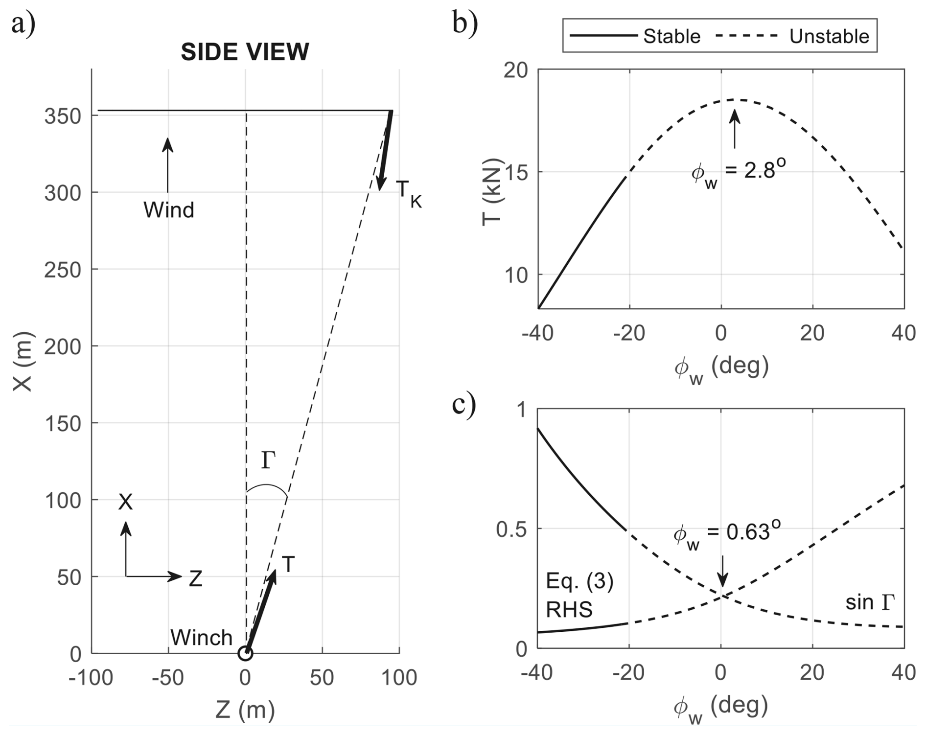
Figure 10 (a) Cone geometry in gravity-free trimmed flight. (b) Tether force at the winch vs reference plane roll angle. (c) Left- and right-hand terms of Eq. (3) vs reference plane roll angle. Note the slight misalignment between T and the cone in panel (a) due to tether sag.

For verification, the results are now cross-checked with prior studies that utilised simplified point-mass models with no tether dynamics. With reference to Fig. 10a, Eq. (2.10) in Trevisi (2024) approximates the relationship between the cone opening angle Γ and the tether force at the aircraft T_K for maximum power production, assuming no gravity. This equation can be reinterpreted in our current coordinate system and notation as

$$\begin{array}{}\text{(2)}& \sin \mathrm{\Gamma }={\displaystyle \frac{m{u}^{\mathrm{2}}}{R{T}_K}},\end{array}$$

where m is the aircraft mass and u is the forward velocity in the body axis. Equation (2) can be improved by including a contribution from the tether weight m_T. Trevisi et al. (2020) suggest lumping the aircraft mass with one-third of the tether weight m_T. This results in

$$\begin{array}{}\text{(3)}& \sin \mathrm{\Gamma }={\displaystyle \frac{(m+m_T/\mathrm{3})u^{\mathrm{2}}}{R{T}_K}}.\end{array}$$

Maximum power is achieved when the tether force at winch T is the highest. Numerical analysis shown in Fig. 7e (reproduced in Fig. 10b) indicates that flying at ϕ_w=2.8° provides the highest T. To compare this result against simplified approximation, the left- and right-hand sides of Eq. (3) are plotted in Fig. 10c as functions of the lean angle ϕ_w. Both terms equal each other when the lean angle is 0.63°. This is very close to the true value of 2.8° – despite the difference between the full and point-mass models – and provides additional confidence in the results shown thus far.

4 Dynamic trim without gravity

The discussed orbits above are all normal to the wind. Circular flights at different angles to the wind require adding energy to the system through the periodic forcing of a control surface – henceforth referred to as “dynamic trim”. Dynamic trim can be achieved through a simple feedback law:

$$\begin{array}{}\text{(4)}& {\mathit{\delta }}_{\mathrm{a}/\mathrm{e}/\mathrm{r}}={\mathit{\delta }}_{\mathrm{a}/\mathrm{e}/{\mathrm{r}}_{\mathrm{0}}}+A\sin {\mathit{\psi }}_{\mathrm{w}},\end{array}$$

where ${\mathit{\delta }}_{\mathrm{a}/\mathrm{e}/\mathrm{r}}$ is one of the three control surfaces, A is a constant in degrees, and ψ_w is the heading angle in the wind plane. ψ_w=0° indicates that the nose is pointing in the positive X_w direction, which is nose vertically up relative to the flat Earth. Subscript 0 denotes the deflection at static trim. In all subsequent discussions, the static trim deflections are $[{\mathit{\delta }}_{{\mathrm{a}}_{\mathrm{0}}}$, ${\mathit{\delta }}_{{\mathrm{e}}_{\mathrm{0}}}$, ${\mathit{\delta }}_{{\mathrm{r}}_{\mathrm{0}}}]=[-\mathrm{1.1}$°, −6.2°, 6.5°], resulting in circular flight at 6° angle of attack, zero sideslip, and ${\mathit{\varphi }}_{\mathrm{w}}=-\mathrm{37}$°.

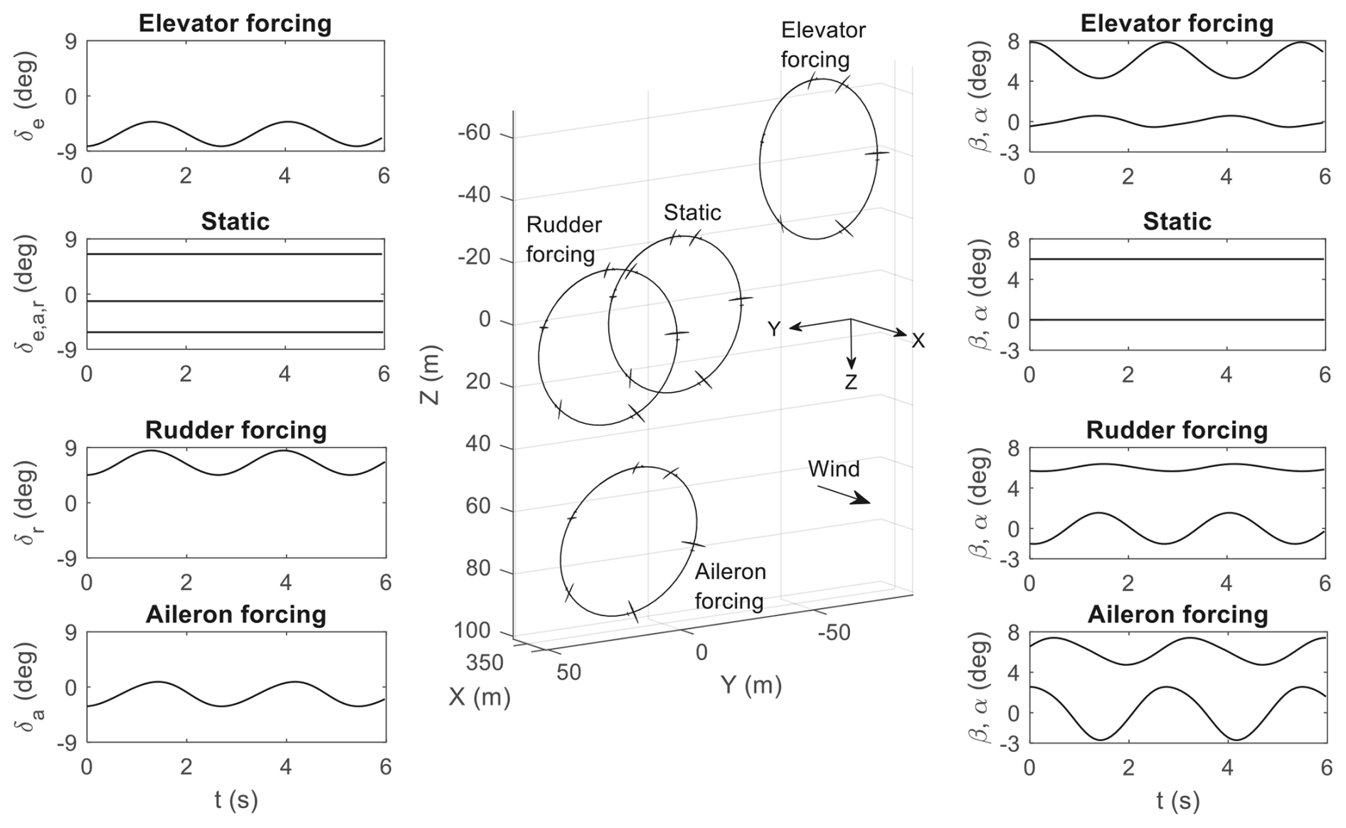
Equation (4) is a way of deflecting a control surface periodically based on the aircraft's position in the orbit. The resulting trajectories are illustrated in Fig. 11 for a forcing amplitude of A=2°. Forcing any of the three available control surfaces has the effect of shifting the circle centre away from its static trim location, thereby achieving circular flight with portions of the orbit flying against the wind. The external forcing also causes oscillations in the aircraft states and outputs due to the apparent wind changing direction periodically.

While all three control effectors could theoretically be used for dynamic trim, it is recommended to use aileron for several reasons. First, aileron forcing frees up the elevator and rudder for pitch and yaw control, respectively. Trevisi (2024) also remarked that actuating the aileron cyclically is a direct way to change the direction of the lift vector from the main wing, thereby providing an effective means to navigate a tethered aerial vehicle in 3D space. This point is supported by a direct comparison between rudder and aileron forcing by Nguyen et al. (2026), which shows that aileron forcing provides superior power-generation capability. Lastly, the circular trajectory of aileron forcing in Fig. 11 is shifted from the static trim location by the largest distance (74.7 m for aileron, 72.3 m for elevator, and 25.8 m for rudder), although the contribution of the large moment arm generated by the long wingspan should be noted.

Figure 11 Dynamic trim at 2° forcing amplitude using different control surfaces.

The effect of changing the forcing amplitude is now investigated. Figure 12 shows that larger A helps to shift the circle further away from its static position, although this comes at a cost of larger variation in all state variables. Another feature to note is that for different values of A, the circles are not simply shifted vertically down but with a slight offset in the positive y direction (not clearly visible in Fig. 12). This can be attributed to the phase lag between when δ_a is deflected and when a change in aircraft response takes effect. Although there is no known direct formula to calculate this continuous phase change, we can compensate for the phase lag by artificially shifting the reference point for ψ_w=0°:

$$\begin{array}{}\text{(5)}& {\mathit{\delta }}_{\mathrm{a}}={\mathit{\delta }}_{{\mathrm{a}}_{\mathrm{0}}}+A\sin ({\mathit{\psi }}_{\mathrm{w}}+\mathrm{\Phi }),\end{array}$$

where Φ is a constant indicating the amount of artificial phase shift. The effect of adding Φ is shown in Fig. 13, where Φ=189° shifts the circle up, with no offset in the y direction. By combining A and Φ, one can move the orbit to a different point in space (subject to physical constraints, such as control power, aerodynamic stall, and sideslip-induced instability).

Figure 12 Effect of changing the forcing amplitude A.

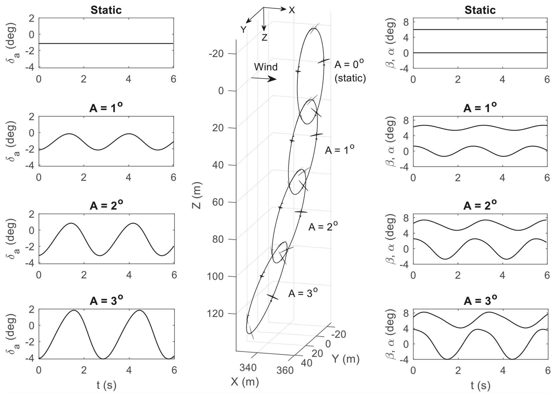
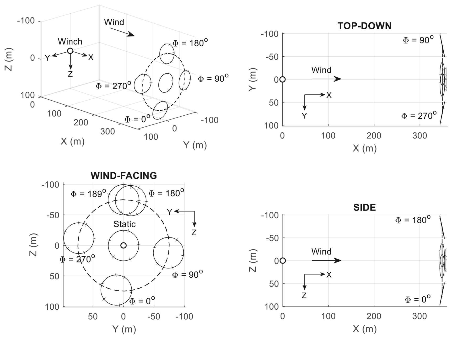
Figure 13 Artificial phase shift at A=2° to move the circle around the original static trim centre.

The oscillation in α and β can be reduced by engaging the elevator and rudder. Using the following proportional feedback law,

$$\begin{array}{}\text{(6)}& \begin{array}{rl}{\mathit{\delta }}_{\mathrm{e}}& ={\mathit{\delta }}_{{\mathrm{e}}_{\mathrm{0}}}+K_{\mathrm{e}}\left(\mathrm{6}-\mathit{\alpha }\right)\\ {\mathit{\delta }}_{\mathrm{r}}& ={\mathit{\delta }}_{{\mathrm{r}}_{\mathrm{0}}}+K_{\mathrm{r}}\left(\mathrm{0}-\mathit{\beta }\right),\end{array}\end{array}$$

where K_e<0 and K_r>0 are proportional gains (negative K_e due to sign convention), and the oscillations can be reduced – as shown in Fig. 14. Furthermore, the circle centre is shifted up, indicating higher aerodynamic efficiency. It can be concluded that there are benefits to reducing the oscillation in α and β during circular flights. Subsequent results will not consider the feedback law in Eq. (6) – the elevator and rudder are static, and only aileron forcing is used.

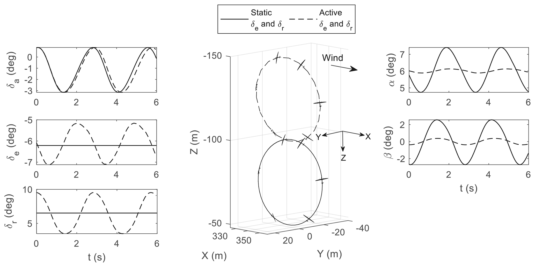
Figure 14 Increased “shifting power” due to reduced α and β oscillation provided by elevator and rudder compensations. Note that $K_{\mathrm{e}}=-\mathrm{2}$, K_r=4, and Φ=189°.

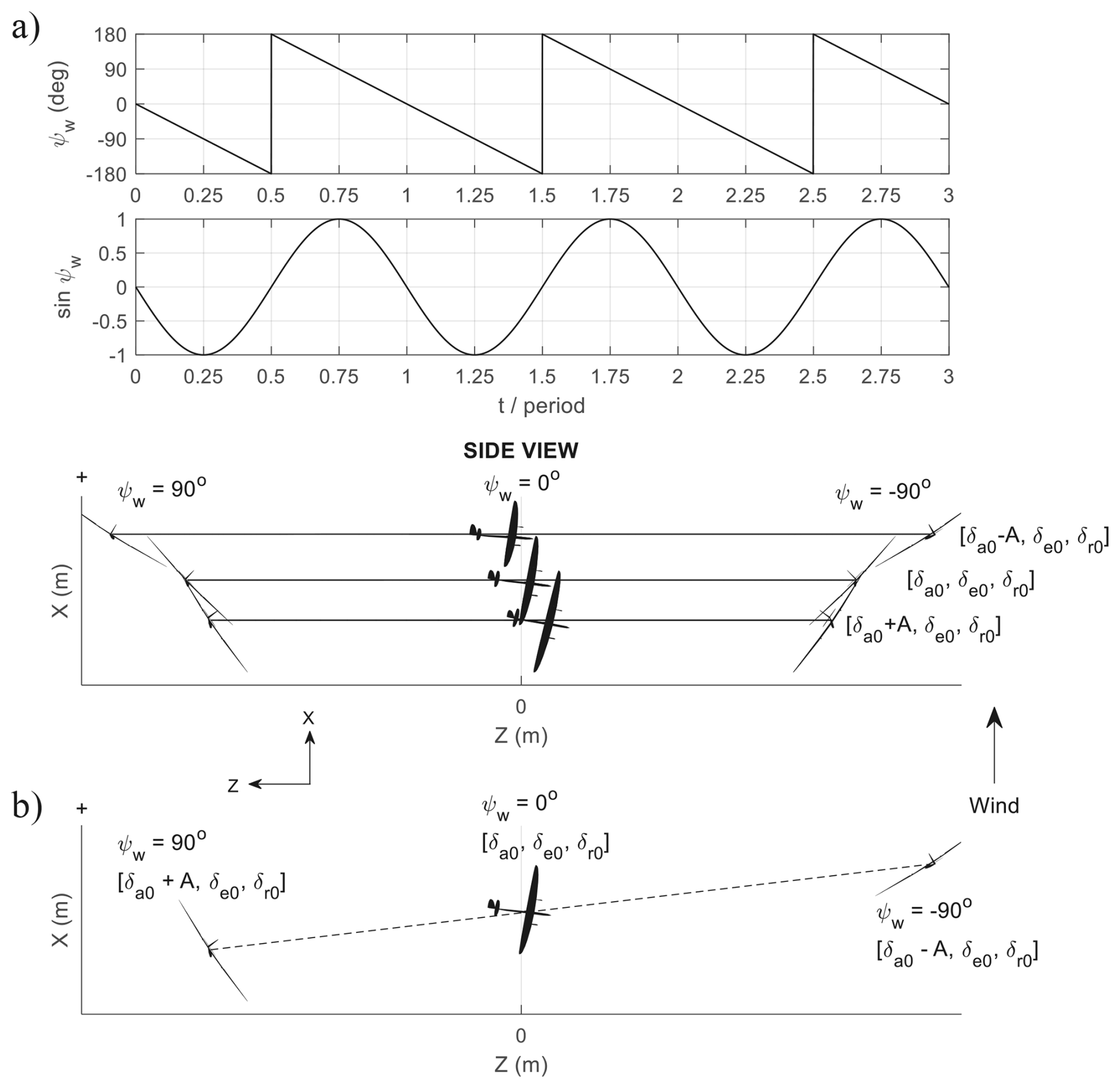
Figure 15 (a) Side view of three generic static trim trajectories (left turning) and their periodic forcing components. Only the middle trajectory is trimmed for zero sideslip. (b) Composite static trim diagram for illustrating the mechanism of dynamic trim.

An explanation of how dynamic trimming works is now provided. Figure 15a shows three example circular trajectories in static trim. The middle orbit is trimmed for zero sideslip at an arbitrary fixed angle of attack. The control surface deflections needed to achieve this trim are $\left[{\mathit{\delta }}_{{\mathrm{a}}_{\mathrm{0}}}{\mathit{\delta }}_{{\mathrm{e}}_{\mathrm{0}}}{\mathit{\delta }}_{{\mathrm{r}}_{\mathrm{0}}}\right]$. On the other hand, the top and bottom orbits experience an aileron offset of ∓A°. As expected, the top trajectory has a wider radius due to more negative (right-roll) aileron trim, while the opposite is true for the bottom trajectory. The top trajectory pulls harder on the tether, leading to more elastic extension and hence flies further away from the winch (the opposite is true if a rigid stick is used to represent the tether: more lean out leads to an orbit closer to the winch). Dynamic trimming using a forcing amplitude of A can be described as the aircraft traversing between the three static trim conditions. Referring to Fig. 15b, when ψ_w is at −90°, the aileron is at its minimum of (${\mathit{\delta }}_{{\mathrm{a}}_{\mathrm{0}}}-A$), while ψ_w=90° gives maximum aileron. Moving between these static trim conditions means periodically changing the radius at different parts of the orbit, causing the circle plane to be angled as seen in Fig. 15b. This also creates an asymmetry in the aerodynamic force at ψ_w=90° and ${\mathit{\psi }}_{\mathrm{w}}=-\mathrm{90}$°, which shifts the circle to the left during dynamic trimming (not shown in Fig. 15). The result is a circular trajectory at a non-90° angle to the wind. Dynamic trimming can also be described from a frequency response perspective. Using Eq. (4), the aileron undergoes harmonic forcing at one of the resonance frequencies (the rate of the aircraft completing one circle). This resonance adds enough energy to the system to enable flying in a circle that is not normal to the wind.

5 Dynamic trim with gravity

Gravity adds an external downforce to both the aircraft and the tether. Consider the static trim case of [${\mathit{\delta }}_{{\mathrm{a}}_{\mathrm{0}}}$, ${\mathit{\delta }}_{{\mathrm{e}}_{\mathrm{0}}}$, ${\mathit{\delta }}_{{\mathrm{r}}_{\mathrm{0}}}$] = [−1.1°, −6.2°, 6.5°], giving ${\mathit{\varphi }}_{\mathrm{w}}=-\mathrm{37}$° (same configuration as in Fig. 11). Figure 16a shows that adding gravity shifts the circle centre of static trim down and to the side, resulting in a plane of orbit that is no longer normal to the wind. The down shift is due to aircraft and tether weights, while the side shift is attributed to the difference in velocity (and hence lift) when the aircraft is travelling up versus down. Both the down and side shifts cause the states and outputs to vary periodically, including α and β, as shown in Fig. 16b.

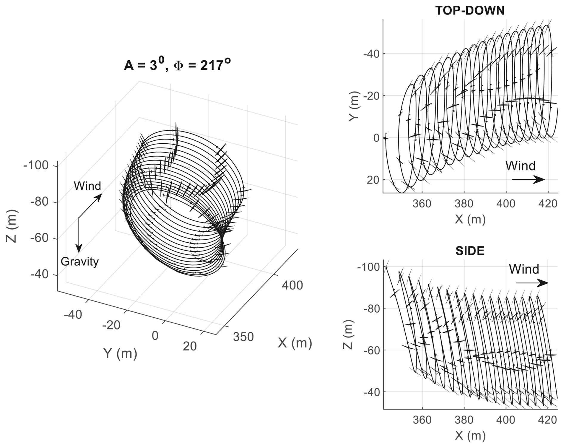
The loci of orbit centres for dynamic trim are also shifted in a similar manner. In Fig. 17, the “contour lines” for the same forcing amplitudes A no longer centre around the origin and become increasingly distorted with higher A, indicating increased non-linearity due to gravity and crosswind. If we seek an orbit above-ground level with no offset in the Y axis, then no such trajectory exists for A=1°. Therefore, a certain level of periodic forcing is required to fly above-ground orbits – especially if there is a minimum height restriction. Results from Fig. 17a indicate that setting A≥2° and Φ around 220° could give a feasible trajectory. To demonstrate, Fig. 18 shows the flight path under aileron forcing, with A=3°, Φ=217°, and an active winch for reel out. The non-zero reel-out rate reduces the relative wind speed at the aircraft, thereby producing less lift and changing the static trim condition. As a result, the flight path sees an immediate height drop and veers off from the Y=0 m centre line. A larger forcing amplitude is therefore needed during reel out to account for lower airspeed while keeping the height above a predefined minimum, and Φ may need to be adjusted with increasing tether length to keep the circle centre around Y=0 m. One way to mitigate the height drop and veering off issues is to reduce the wind speed for all analyses involving a fixed tether length. The reduction amount should be selected so that the airspeed seen by the aircraft at a fixed tether length (winch inactive) is similar to the airspeed experienced with the winch active.

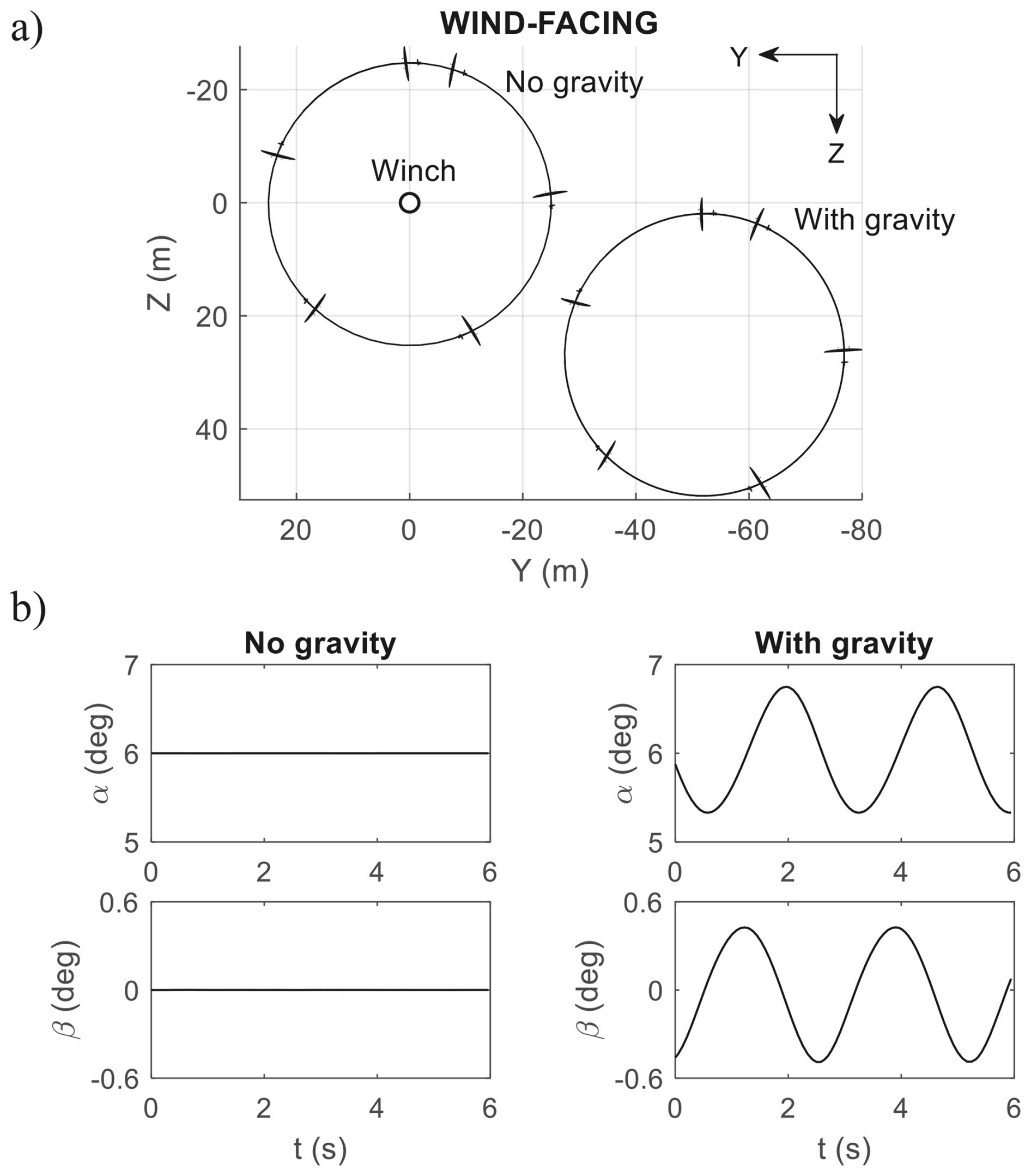
Figure 16 Effect of gravity on static trim: (a) trajectory and (b) time histories. The wind direction in panel (a) is out of the page.

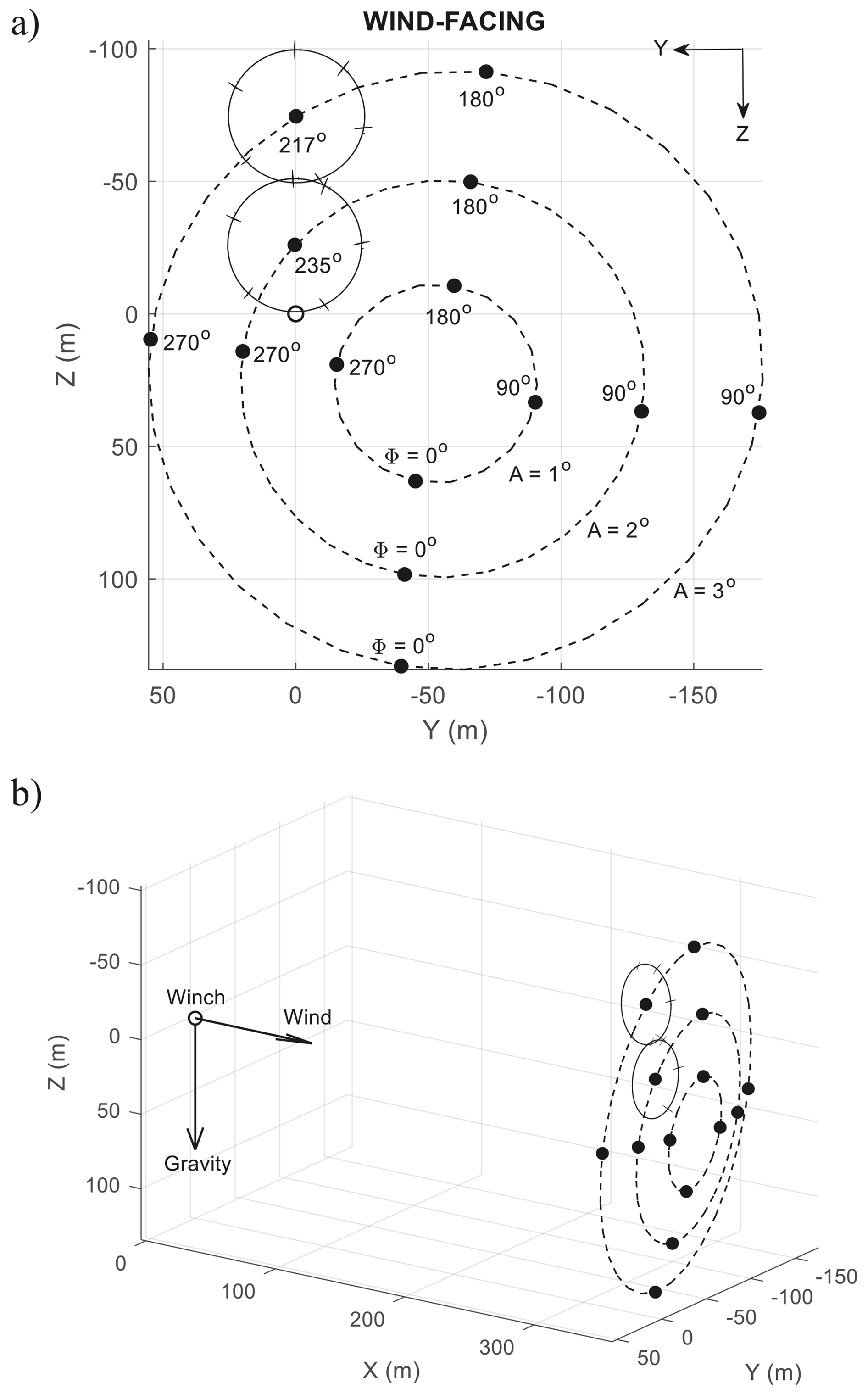
Figure 17 Loci of orbit centres (dashed lines) at different forcing amplitudes A in the presence of gravity. Two example orbits are drawn in solid lines. Figure shows both (a) 2D and (b) 3D projections.

Figure 18 Reel out with dynamic trim (aileron forcing – Eq. 5).

6 Conclusions

The mechanism of circular flight in rigid-wing tethered aircraft has been examined. Static trim analysis (no moving control surface) in a gravity-free environment shows that lean angle determines the orbit radius, and the highest tether tension is achieved at a lean angle slightly above zero. Static stability may be lost when the lean angle exceeds a critical value, although artificial stabilisation can be done through cross-feeding pitch and roll into the aileron. In the presence of gravity, the orbit centre can be adjusted through periodic forcing of one of the control surfaces – most effectively, the aileron. The proposed dynamic trimming law could be used in a simulation environment to determine whether an aircraft has suitable control power to achieve circular flights. Such a test is suitable for verifying an early-stage design, especially when a full flight control system is not available. For test flights, a more sophisticated algorithm is recommended to account for non-uniform wind that may have a vertical component. The dynamic trimming concept can also be expanded to construct a full reel-out flight control system for rigid-wing AWESs.

Appendix A: Practical considerations for analyses involving numerical continuation

This section outlines a few numerical challenges involving time simulation and numerical continuation of the airborne wind system considered. A few methods to remedy those issues are also proposed.

Figure A1 A typical time history of the heading angle during circular motion.

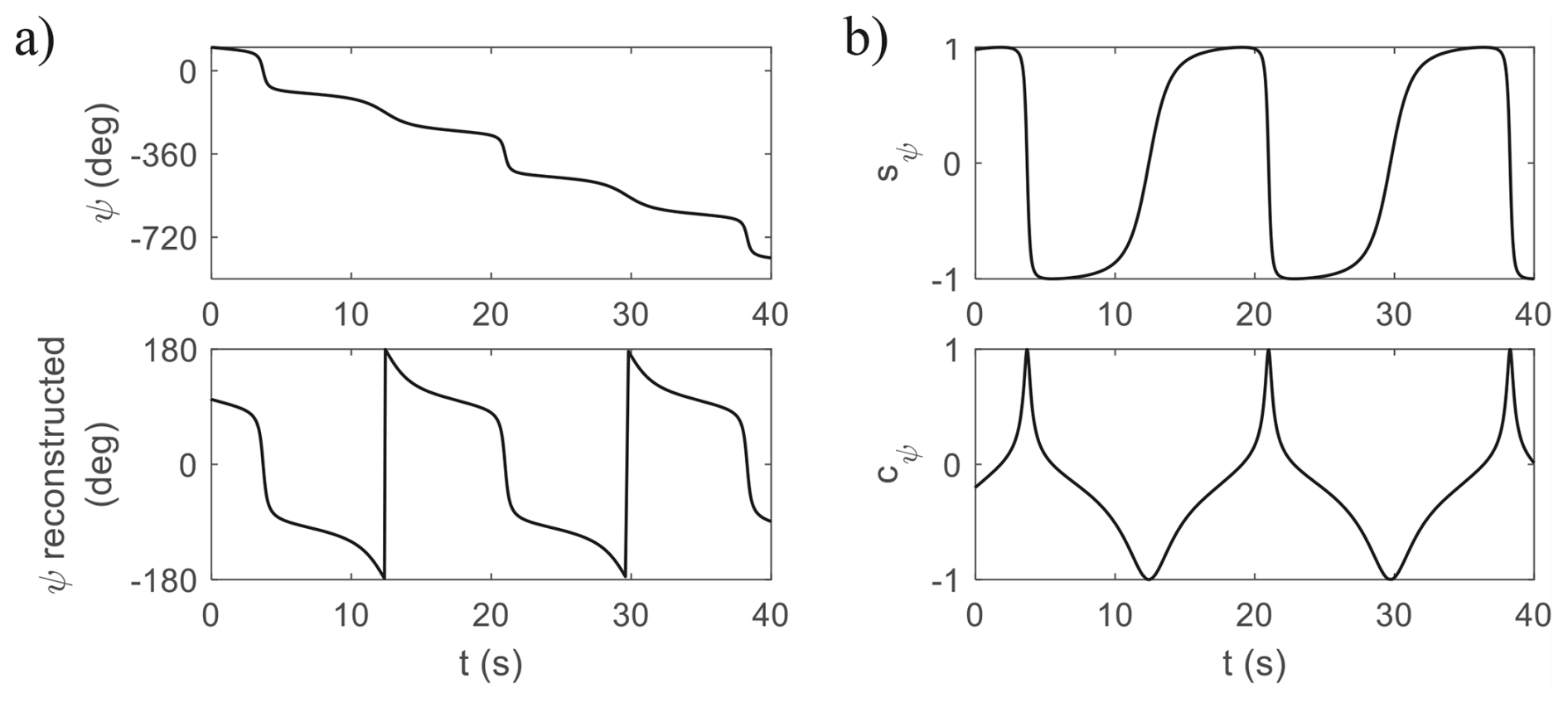
First, the heading angle ψ in the Earth frame tends to increase monotonically when the aircraft flies a circular orbit oriented close to 90° to the ground, such as in Fig. 5. The resulting ψ time history is shown in the top half of Fig. A1. A dynamical system with such a response is not considered periodic (repeating) and hence cannot be solved by the numerical continuation software AUTO. However, the sine and cosine of ψ is periodic. We can decompose ψ into two states s_ψ and c_ψ based on the Hopf normal form

$$\begin{array}{}\text{(A1)}& \begin{array}{rl}{\dot{s}}_{\mathit{\psi }}& =s_{\mathit{\psi }}+\dot{\mathit{\psi }}{c}_{\mathit{\psi }}-s_{\mathit{\psi }}\left(s_{\mathit{\psi }}^{\mathrm{2}}+c_{\mathit{\psi }}^{\mathrm{2}}\right)\\ {\dot{c}}_{\mathit{\psi }}& =c_{\mathit{\psi }}-\dot{\mathit{\psi }}{s}_{\mathit{\psi }}-c_{\mathit{\psi }}(s_{\mathit{\psi }}^{\mathrm{2}}+c_{\mathit{\psi }}^{\mathrm{2}}),\end{array}\end{array}$$

where the rate of change of ψ follows the definition from the literature.

$$\begin{array}{}\text{(A2)}& \dot{\mathit{\psi }}=q{\displaystyle \frac{\sin \mathit{\varphi }}{\cos \mathit{\theta }}}+r{\displaystyle \frac{\cos \mathit{\varphi }}{\cos \mathit{\theta }}}\end{array}$$

Here, s_ψ and c_ψ represent sin ψ(t) and cos ψ(t), respectively. This interpretation works because as long as the initial conditions for s_ψ and c_ψ satisfy the physical constraint $s_{\mathit{\psi }}^{\mathrm{2}}+c_{\mathit{\psi }}^{\mathrm{2}}=\mathrm{1}$, Eq. (A1) reduces to

$$\begin{array}{}\text{(A3)}& \begin{array}{rl}{\dot{s}}_{\mathit{\psi }}& =\dot{\mathit{\psi }}{c}_{\mathit{\psi }}\\ {\dot{c}}_{\mathit{\psi }}& =-\dot{\mathit{\psi }}{s}_{\mathit{\psi }},\end{array}\end{array}$$

which is identical to

$$\begin{array}{}\text{(A4)}& \begin{array}{rl}{\displaystyle \frac{\mathrm{d}}{\mathrm{d}t}}\left(\sin \mathit{\psi }\right)& =\dot{\mathit{\psi }}\cos \mathit{\psi }\\ {\displaystyle \frac{\mathrm{d}}{\mathrm{d}t}}\left(\cos \mathit{\psi }\right)& =-\dot{\mathit{\psi }}\sin \mathit{\psi }.\end{array}\end{array}$$

It is worth noting that Eq. (A1) is numerically stable, whereas Eq. (A3) is not. This means that assuming the system with the original equation for $\dot{\mathit{\psi }}$ is stable, its representation using Eq. (A1) is also stable, as a perturbation to either state in Eq. (A1) will be damped out, bringing the trajectory back to the same attractor. This “restoring force” is provided by the cancelled-out terms in Eq. (A1) when $s_{\mathit{\psi }}^{\mathrm{2}}+c_{\mathit{\psi }}^{\mathrm{2}}=\mathrm{1}$. If these terms are removed, as in Eq. (A3), a perturbation to either state in Eq. (A3) will cause instability. The continuation software AUTO cannot solve for the system with Eq. (A3), but can work with Eq. (A1). In both cases, as long as the physical constraint $s_{\mathit{\psi }}^{\mathrm{2}}+c_{\mathit{\psi }}^{\mathrm{2}}=\mathrm{1}$ is maintained, the trajectory will be identical to that of the original system. Figure A1b shows the dynamics of Eq. (A1) when the physical constraint is satisfied. From here, the heading angle wrapped between $-\mathit{\pi }/\mathrm{2}$ and $+\mathit{\pi }/\mathrm{2}$ can be reconstructed using an atan2 function, as shown in the lower half of Fig. A1a.

Figure A2 Euler angles of two circular orbits, with θ and ϕ close to ±90°.

In gravity-free analyses, such as in Fig. 6, the roll angle ϕ may also increase monotonically in a similar manner to Fig. A1. The Hopf normal form can be used again, replacing $\dot{\mathit{\psi }}$ with $\dot{\mathit{\varphi }}$ to hide ϕ in two states representing sin ϕ and cos ϕ.

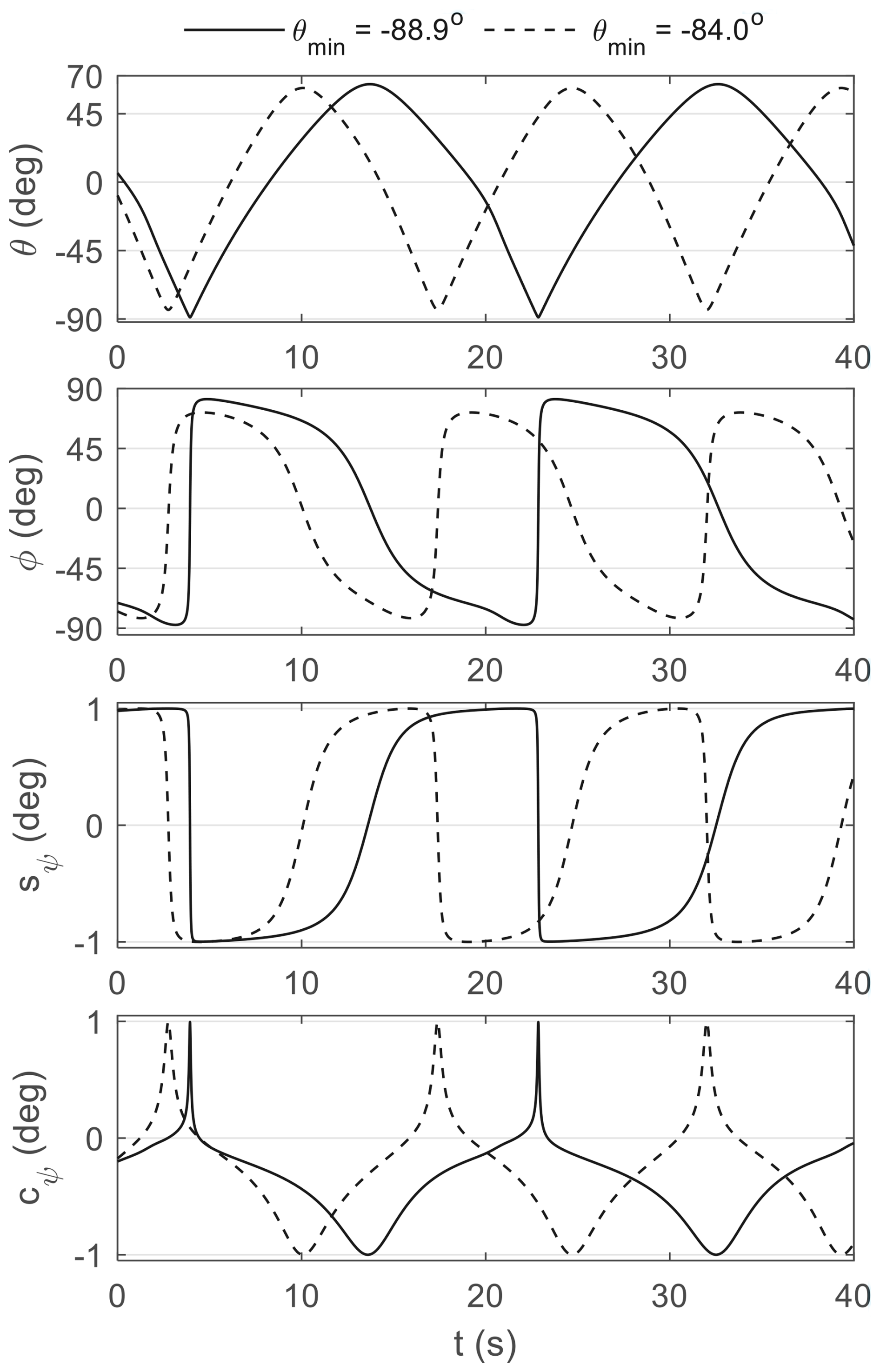
The second issue is numerical stiffness. This is due to the pitch angle θ in the Earth frame regularly approaching or crossing ±90° during circular motion. From the definitions of ψ (see Eq. A2), as θ approaches ±90°, $\mathrm{1}/\cos \mathit{\theta }$ approaches infinity. A similar problem is present in the roll angle ϕ:

$$\begin{array}{}\text{(A5)}& \dot{\mathit{\varphi }}=p+q{\displaystyle \frac{\tan \mathit{\theta }}{\sin \mathit{\varphi }}}+r{\displaystyle \frac{\tan \mathit{\theta }}{\cos \mathit{\varphi }}},\end{array}$$

which tends to infinity as tan θ approaches 90°. The consequence is a very rapid change of direction in the Euler angle states. Figure A2 illustrates the issue by comparing two circular orbits with the same tether lengths but different radii. The solid-line trajectory has a minimum pitch angle of −88.9°, which is only 4.9° less than that of the dashed-line trajectory. Although the difference is small, its impact on the numerical solver is evident. This leads to a stiff system that requires small step sizes, sometimes enough to fail the continuation solver.

A possible remedy is to use vertical instead of horizontal wind in gravity-free cases. The resulting trajectories are identical but at 90° to each other. With vertical wind, the Earth frame coincides with the wind frame, resulting in the states ϕ and θ admitting equilibrium (static trim) or small-amplitude oscillations close to zero (dynamic trim). This significantly reduces the computation cost for both time integration and continuation.