An experimental campaign to measure turbulence in the marine boundary layer

There is a lack of measurement data on the spatial structure of turbulence at heights greater than 100 m in the marine atmospheric boundary layer (MBL). Consequently, turbulence models like the Mann and Kaimal models, which are referred to in industry standards, have not been validated at the operational heights of large offshore wind turbines. To address this gap, we carried out an experimental campaign using a total of five lidars placed at two locations on the west coast of Denmark. This setup allowed us to measure the horizontal wind components at the intersections of the lidar beams which were 150 to 250 m above the sea surface. As a result, lateral coherence can be assessed up to separations of 240 m. Due to differences in data quality from each lidar, the data availability at each intersection point was different, being in the range between 17 % and 50 % over the entire 360° sector. Thus, this measurement dataset can be used to test and validate turbulence models in the MBL at heights relevant for offshore wind turbines.

1 Introduction

Wind turbines are expected to continually increase in size over the next few decades. But there are many open research questions that must be addressed in order to bring about the expected decrease in cost of wind energy. One of these concerns the modeling of turbulence at the heights of multi-megawatt wind turbines (Kuik et al., 2016; Veers et al., 2023). The Kaimal (Kaimal et al., 1972) turbulence model was designed for onshore turbulence within the atmospheric surface layer, and the Mann (1994) model was validated, both on and offshore, but only to heights less than 100 m. Consequently, the assumptions behind these models may be violated at higher heights in the marine atmospheric boundary layer (MBL). For instance, both models assume that a large spectral gap exists between meso-scale and micro-scale turbulence. Moreover, the Kaimal model uses the vertical coordinate as length scale, which also limits its vertical range of applicability. There is also a lack of measurement data against which newer turbulence models (e.g., Segalini and Arnqvist, 2015; Chougule et al., 2017; Syed and Mann, 2024) can be validated.

Measurements of turbulence in the MBL have an extensive history in the field of atmospheric research (Weiler and Burling, 1967; Lenschow and Agee, 1976; Lenschow and Stankov, 1986; Wyngaard, 1992) and, more recently, in the context of wind energy (Cheynet et al., 2017; Lampert et al., 2020; Putri et al., 2022; Syed and Mann, 2024). One of the first campaigns to measure turbulence at heights of modern wind turbines was carried out by Mann et al. (1991). They measured two-point co-spectra in the marine boundary layer using two meteorological masts (met-masts) placed on the island of Sprogø in the Great Belt, Denmark. Vincent et al. (2013) and Larsén et al. (2013) analyzed spectra, co-spectra, and coherence at low frequencies and at separations of more than 1 km from two wind farms in the North and Baltic seas. More recently, Cheynet et al. (2018) computed the spectra and vertical coherence over different stability regimes at heights up to 81 m above the German North Sea. They found that the Kaimal model mostly matched the observed spectra, except under very stable conditions when low-frequency mesoscale turbulence was present in the frequency range under investigation. The vertical coherence was also found to be adequately described by the Davenport model (Davenport, 1961).

Due to the high cost of tall offshore met-masts, remote sensing techniques such as light detection and ranging (lidar; see Sathe and Mann, 2013) have been increasingly used to measure turbulence at higher altitudes in the MBL (Cheynet et al., 2016, 2021; Angelou et al., 2023; Syed and Mann, 2024). Short-range continuous-wave dual lidars were deployed by Cheynet et al. (2016) on a bridge in Norway at a height of 55 m to measure lateral coherence, demonstrating that spatial averaging effects of lidars were negligible for these coherence measurements. Later a triple lidar configuration was used on the same platform, with the third lidar placed on the ground, to study coherence for both lateral and vertical separations (Nafisifard et al., 2023). Building on the dual lidar layout, Cheynet et al. (2021) used long-range scanning pulsed lidars to record spectra and lateral coherence up to 130 m above the Norwegian Sea in what was called the COTUR (COherence of TURbulence with lidars) campaign. However, high uncertainty in beam pointing directions limited the accuracy of their results. Angelou et al. (2023) and Syed and Mann (2024) used forward-looking nacelle lidars to measure lateral coherence at separations of around 100 m above the sea. These studies also observed meso-scale turbulence with the characteristic $-\mathrm{5}/\mathrm{3}$ slope (Nastrom et al., 1984; Lindborg, 1999) but were limited to line-of-sight measurements.

Here, we describe an experimental campaign aimed at measuring turbulence 150 and 250 m above the North Sea. Our setup consists of five lidars placed on the western coast of Denmark. Moreover, the lidar beam directions are calibrated via drones to achieve a high pointing accuracy. It allows the lateral coherence in the “true” wind components to be measured at such heights, which has not been achieved before. The paper is structured as follows. Section 2 provides details of the experimental campaign including the site, instrumentation and calibration procedures. Section 3 describes what is contained in the publicly available data repository, and Sect. 4 presents some quality checks on the data.

2 The field campaign

2.1 Measurement layout overview

Like the COTUR experiment (Cheynet et al., 2021), we chose a coast facing the prevailing wind with a long uninterrupted offshore upstream fetch and relatively low terrain behind the shore in order to emulate offshore conditions undisturbed by topography since a real offshore site would have been too expensive to install and operate. Such a coastal site was already located in the RUNE experiment (Floors et al., 2016), which investigated near-shore flow with lidars, and we reuse that site here. From the RUNE experiment, we already knew that landowners, tourists, and neighbors were positively inclined and would do no harm to the instrumentation. An additional practical advantage was the proximity to DTU's wind turbine test station at Høvsøre (Peña et al., 2016) that could provide some background meteorological information and the presence of technicians who could check the experiment regularly. Finally, this region of the North Sea is very close to planned and operating wind farms making the measurements even more relevant.

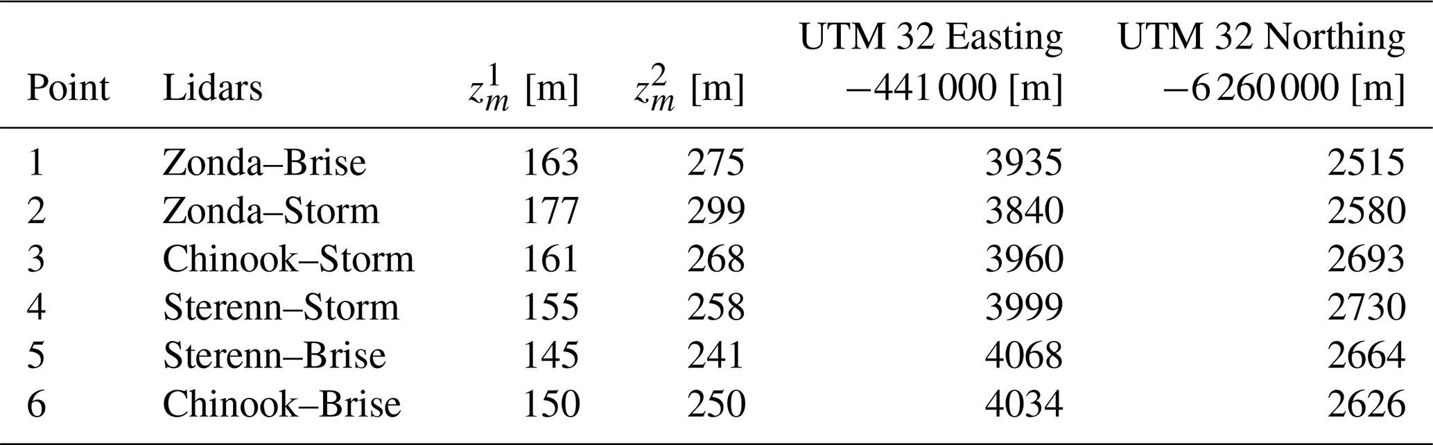
The experimental setup is shown in Fig. 1. A total of five lidars were used in the experiment wherein two lidars were placed at the northern site close to the lighthouse in Bovbjerg and three lidars were present next to the church in Trans. The beams were pointed in westerly directions and had relatively low elevation angles (maximum 6.6° in phase 1 and 11.8° in phase 2) which meant that the plane of intersection lay about 150 m above the sea surface during the first phase of the campaign. The beam elevations were increased midway through the campaign, moving the intersection points to approximately 250 m. The precise elevation angles are described in Table 2, the height of the intersection points are shown in Table 5, and a closer view of the intersection points is shown in Fig. 2.

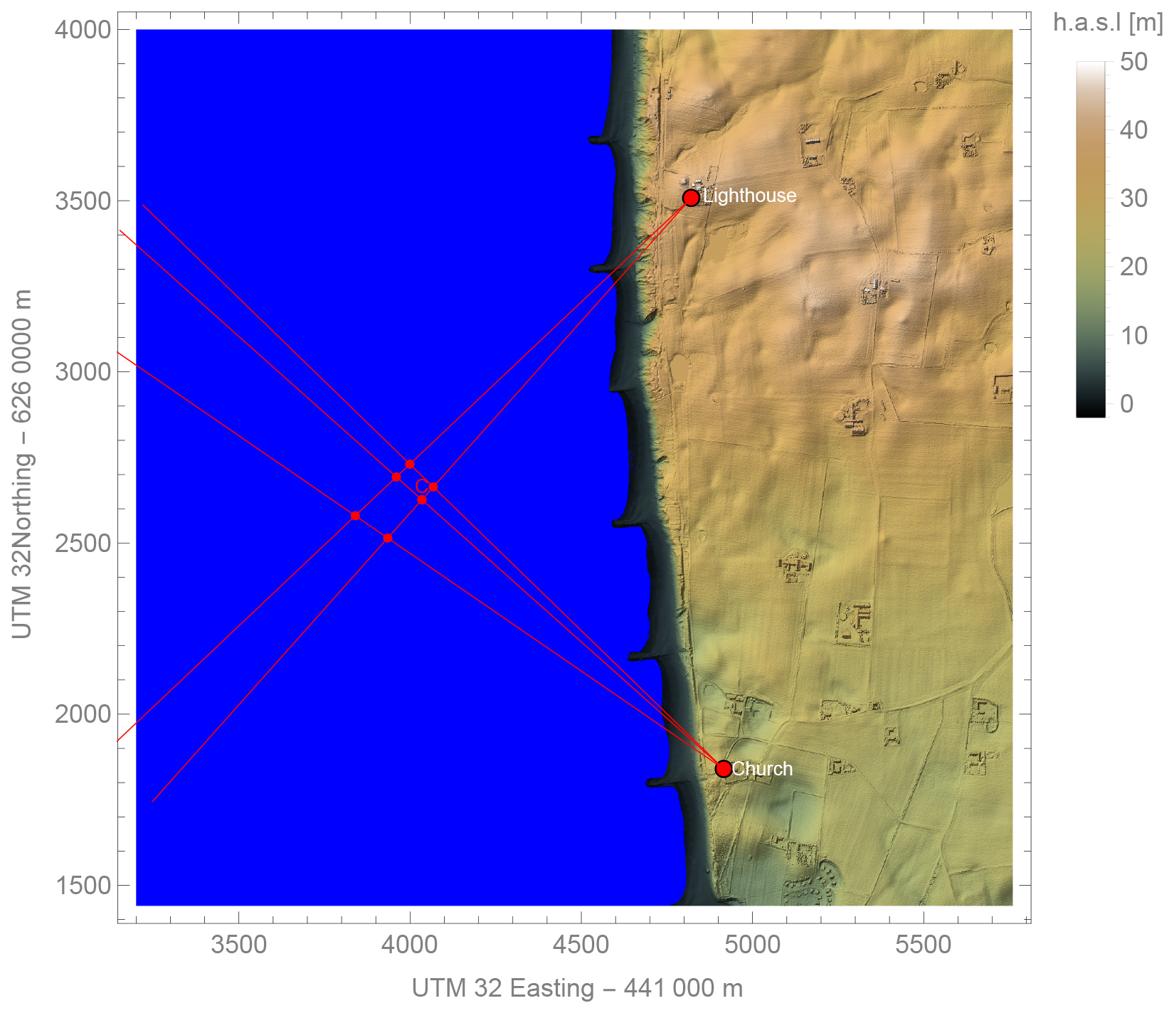
Figure 1 Top view of the experiment showing the two sites next to the church and the lighthouse. The lidar beams are shown in red while the dots indicate the intersection points. The center point where the beams meet at a 90° azimuth angle is indicated by a “C”. The height above sea level is abbreviated by h a.s.l.

Figure 2 The intersection points of the lidar beams. The coordinates are given in Table 5.

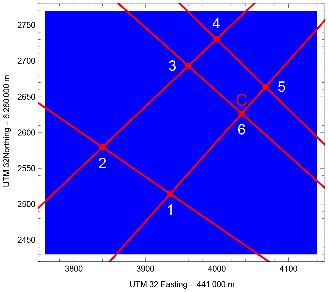
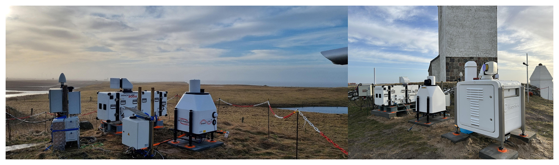
Figure 3 Photos of the two sites where equipment was deployed in the field campaign (left: lighthouse, right: church).

The timeline of the pre-campaign and experimental field campaign, which included two staring configurations, is presented as a Gantt diagram in Fig. 4. In this diagram, longer periods are represented by bars, while shorter events are indicated by circles. Before the measurement campaign was started, pre-campaign instrumentation testing and verification was conducted at the Risø site. A detailed description of this test and verification can be found in Sect. 2.3. During the measurement campaign, the alignment of the scanners was verified using several methods, including hard target mapping (see Sect. 2.3.1), sea surface leveling verification (see Sect. 2.3.3), and drone-based pointing verification (see Sect. 2.3.2). The original plan was to perform drone-based alignment checks at the beginning, midpoint, and end of the campaign. However, due to technical issues with the drone, the mid-campaign check could not be carried out. Instead, sea surface leveling verification was conducted in April. This revealed a significant deviation in the elevation angle for some of the scanners (see Table 8). Consequently, it was decided to correct the elevation angle for staring configuration 2 based on the error identified from the sea surface leveling verification. At the conclusion of the measurement campaign, a line-of-sight (LOS) speed inter-comparison was performed, during which it was found that two of the lidars exhibited significant LOS offsets. A detailed description of this inter-comparison is provided in Sect. 2.3.4.

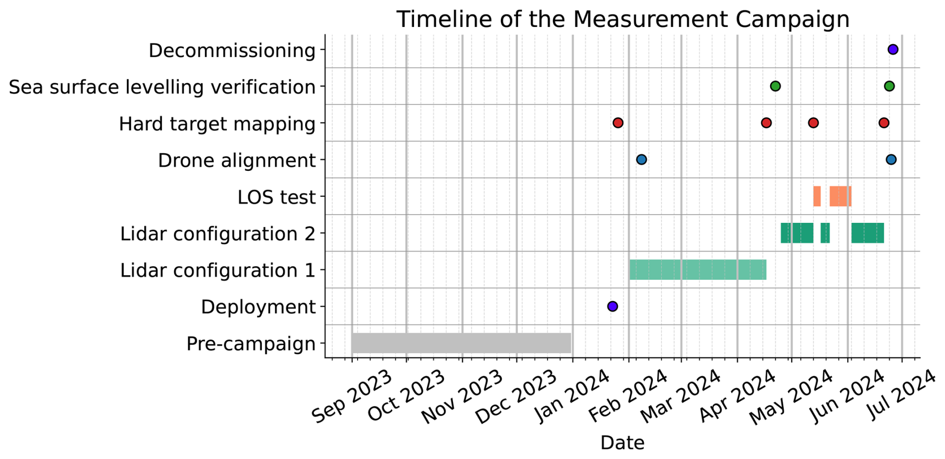
Figure 4 Timeline of the project. Longer periods are marked with a bar, whereas shorter events are marked with a circle.

2.2 Measurement instrumentation and configurations

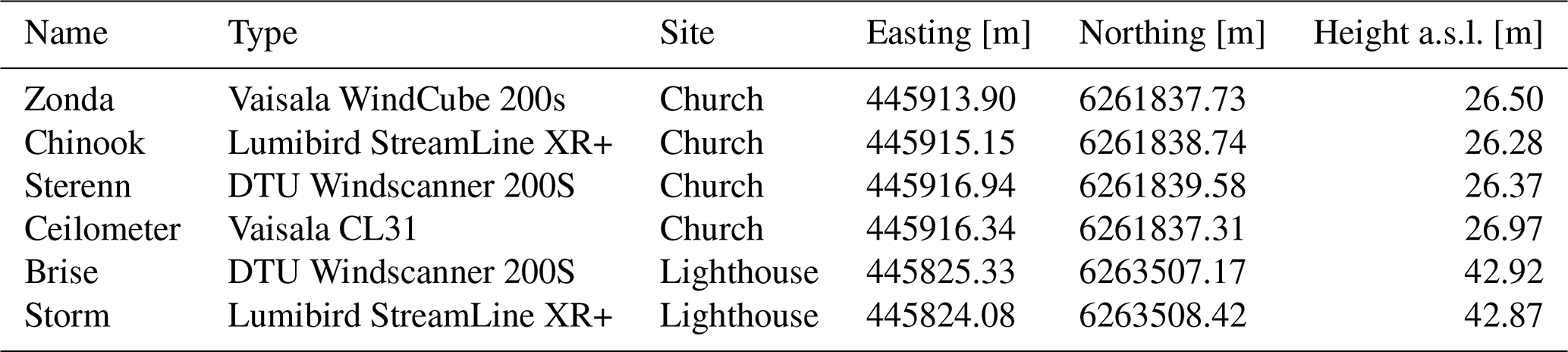
The southern instrumentation site (Trans Church) has a Vaisala CL31 ceilometer and three scanning pulsed lidar systems: one Vaisala WindCube Scan 200S, one Lumibird AllSky Streamline XR+, and one DTU Long-Range WindScanner 200S (see Fig. 3). The northern instrumentation site (Bovbjerg lighthouse) has two scanning pulsed lidar systems (one Streamline XR+ and one Long-Range WindScanner 200S). The positions of the equipment are in global GPS WGS84 UTM zone 32V coordinates and are listed in Table 1.

Table 1 Positions of the equipment acquired using a Leica GS16 GNSS antenna in global GPS coordinates within UTM zone 32V. Positions refer to the center of the beam exit window.

The scanning lidar systems are configured to operate in staring (line-of-sight, LOS) mode, with fixed azimuth and elevation angle. During the campaign two different staring configurations were used. Table 2 shows the configurations of the different scanners.

Time synchronization between data recorded by each lidar has been achieved using the lidars' internal GPS modules, which continuously synchronize the internal clock to a global reference time. All systems were set to UTC time zone with no daylight savings shift. During the campaign, the system clocks were monitored to ensure correct alignment and to detect potential software issues as was experienced and resolved during pre-campaign testing.

Table 2 Summary of scanner setup. Beam directions are given in the global coordinate system.

^a For Streamline XR+ systems, the minimum useful range is approximately 50 m due to window reflection. ^b The probe length is for the Streamline XR+ systems given as the gate length (Halo Photonics (Lumibird Group), 2026) using 8 points and the WindScanner (Vasiljević et al., 2016) and Windcube uses the smallest possible probe length (Vaisala/Leosphere, 2015). The sampling rate was 1 Hz for Zonda and 2 Hz for the remaining scanners.

2.3 Pre-campaign instrumentation testing and verification

The pre-campaign testing and verification activities were carried out at DTU's Risø campus in Denmark, where five scanning lidars were deployed, four of which were used in the campaign (see Fig. 5). The purpose of the pre-campaign testing was to ensure the correct functioning of the lidars and to determine if any offsets were present in the measurement data. As demonstrated in Simon et al. (2023), it is critical to perform these tests to ensure consistent and traceable performance of the lidar instruments. One of the scanners that was tested in the pre-campaign suffered a fatal laser error and was therefore not used in the rest of the campaign. A replacement lidar (Zonda) was deployed in the measurement campaign in Jutland but was not part of the pre-campaign testing. The five scanning lidars were deployed side-by-side at the turbine test station. The work began with calibrating the lidars' internal inclinometers to determine the value of the sensor readout (pitch and roll angles) which correspond to the level position of the lidar. This was accomplished by placing survey sticks with known positions across a range of azimuth positions and using each lidar's hard target mapping function to locate each stick in the lidar coordinate system. The leveling error was then determined, and the lidar was adjusted accordingly. This process was repeated until the stick positions were aligned in both the lidar coordinate system (found by hard-targeting) and global coordinate systems (calculated using the measured GPS positions) at all positions for all lidars. The inclinometer calibration method follows the procedure described in Thorsen et al. (2023) and Gómez et al. (2023).

Next, the lidars were set to measure in fixed LOS staring mode, with their beams placed in parallel, aimed and centered 1 m above the 118 m cup anemometer sensor on the 125 m tall Risø met-mast (Sogachev and Dellwik, 2017). The beam alignment was confirmed using hard-target mapping. However, the wind measurements taken during this period were of limited use due to hardware issues which were present on the Streamline XR+ systems. The issues included water ingress into one lidar due to improper weatherproofing of the lidar casing and a misadjusted focus position on both systems during manufacturer servicing, which led to poor range and data availability during the tests. The Streamline systems were sent back to the manufacturer and repaired under warranty. Time synchronization was also an issue at the start of the tests for the WindScanner systems due to a software incompatibility with the Meinberg GPS module and Windows 10. The time-synchronization issue was resolved with a software update on 18 October 2023 at 09:09:20 UTC and the timestamps from this point forward are aligned and synchronized between all equipment.

Although the pre-campaign test was originally designed as a line-of-sight (LOS) inter-comparison of all four available scanning lidars, with a plausibility check against the met-mast, the measurements had to be collected during separate test periods. As a result, no concurrent dataset exists in which all four lidars and the met-mast were operating simultaneously. The primary objective of this pre-campaign test was to verify the consistency between the lidar systems that would later be used in the dual-Doppler configuration, rather than to establish an absolute calibration against the met-mast. A secondary objective was to confirm that the planned scan configuration for the turbulence measurements would reach sufficient range during the main campaign. Due to the internal humidity and focus issues mentioned previously, the measurement range of the two Streamline systems did not reliably reach the met-mast (1 km), so only a small number of valid samples were obtained directly at the mast location. Consequently, only the LOS considered for the WindScanner systems (Fig. 6, left) reached the met-mast. For the Streamline systems, we selected the range gate at 450 m, where both systems, despite their different failure causes, still provided sufficient signal quality to allow a reliable LOS comparison. The met-mast data used in the pre-campaign analysis should therefore not be interpreted as a calibration ground truth, particularly because they were collected before the repair and major maintenance of the Streamline systems but rather only as an additional plausibility check.

For the LOS inter-comparisons shown in Fig. 6, we applied a simple quality-control procedure before computing the 10 min averages. For the WindScanner systems, all LOS samples with carrier-to-noise ratio (CNR) ≤−22 dB or with retrieved LOS wind speed outside the interval [−40, 40] m s⁻¹ were discarded. For the Lumibird systems, we required an intensity larger than 1.009 and applied the same [−40, 40] m s⁻¹ LOS wind-speed filter. Short periods with clear outliers were also excluded. Only LOS data that passed this quality control were used in the calculation of the 10 min mean wind speeds. Furthermore, a constant time shift was applied to each system pair, where necessary, before performing the aggregation in order to minimize systematic timing errors. Due to incompatibilities of the Meinberg GPS module, the effective time offset was not constant but varied over the pre-campaign period and between systems. For the WindScanner systems, this resulted in average corrections of 3750 s for Brise and 3620 s for Sterenn relative to UTC time, derived from the mean offset over the testing period up to 18 October 2023 at 09:09:20 UTC. These corrections remove the bulk time mismatch, although residual time lags may still remain. No significant time shifts were identified between the Streamline systems. Lastly, in the regression analysis we only included 10 min intervals for which at least 80 % of the scheduled LOS measurements were valid for each of the two lidar systems.

For both WindScanner systems, the met-mast was reachable during the testing period, enabling a comparison between the lidar LOS wind speed and the cup anemometer and wind vane measurements projected onto the lidar LOS, as shown in Fig. 7. The above-mentioned quality-control procedure was applied to the LOS wind speeds and to the 10 min aggregation. Additionally, to minimize potential cross-wind component contamination, we retained data only when the wind direction was within ±40° of the LOS or within ±40° of the opposite direction (180° offset), according to International Electrotechnical Commission (2022). This wind direction selection also excludes the sector influenced by met-mast wake effects. Under these conditions, projection errors from the wind vane can be better distinguished and further compensated for. To mitigate the impact of a wind direction offset on the projection, a sinusoidal function was fitted to the wind-speed ratio ($V_{\mathrm{LoS}}/V_{\mathrm{cup}}$) as a function of the azimuth angle in order to determine the lidar LOS angle in the wind vane coordinate system. This analysis uncovered a directional offset of the wind vane relative to the scanning lidar. The fitting process was applied to each system, and the outcomes from the Sterenn system were selected for consistency across systems. An angular offset of 5.8° was applied uniformly to all systems when using the met-mast cup anemometer as a reference. Sterenn was installed centrally among all scanning lidars, which justified the findings and the choice of this angular offset to ensure consistency. The results shown in Fig. 7 reflect this filtering and correction, with the corresponding regression-derived offsets summarized in Table 3.

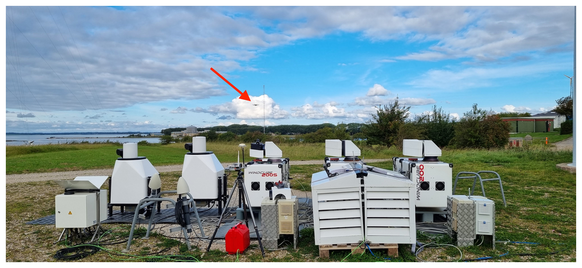
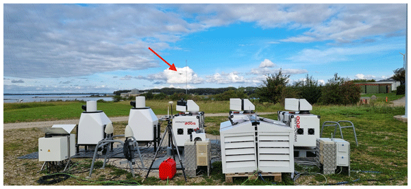
Figure 5 Photo of the pre-campaign lidar tests at Risø test station. A telescopic sight is fitted to the system in the center to help align the scan head with the met-mast and drone. The drone is flying and is visible in the center of the image at the red arrow.

Table 3 Results from the onshore pre-campaign line-of-sight speed calibration.

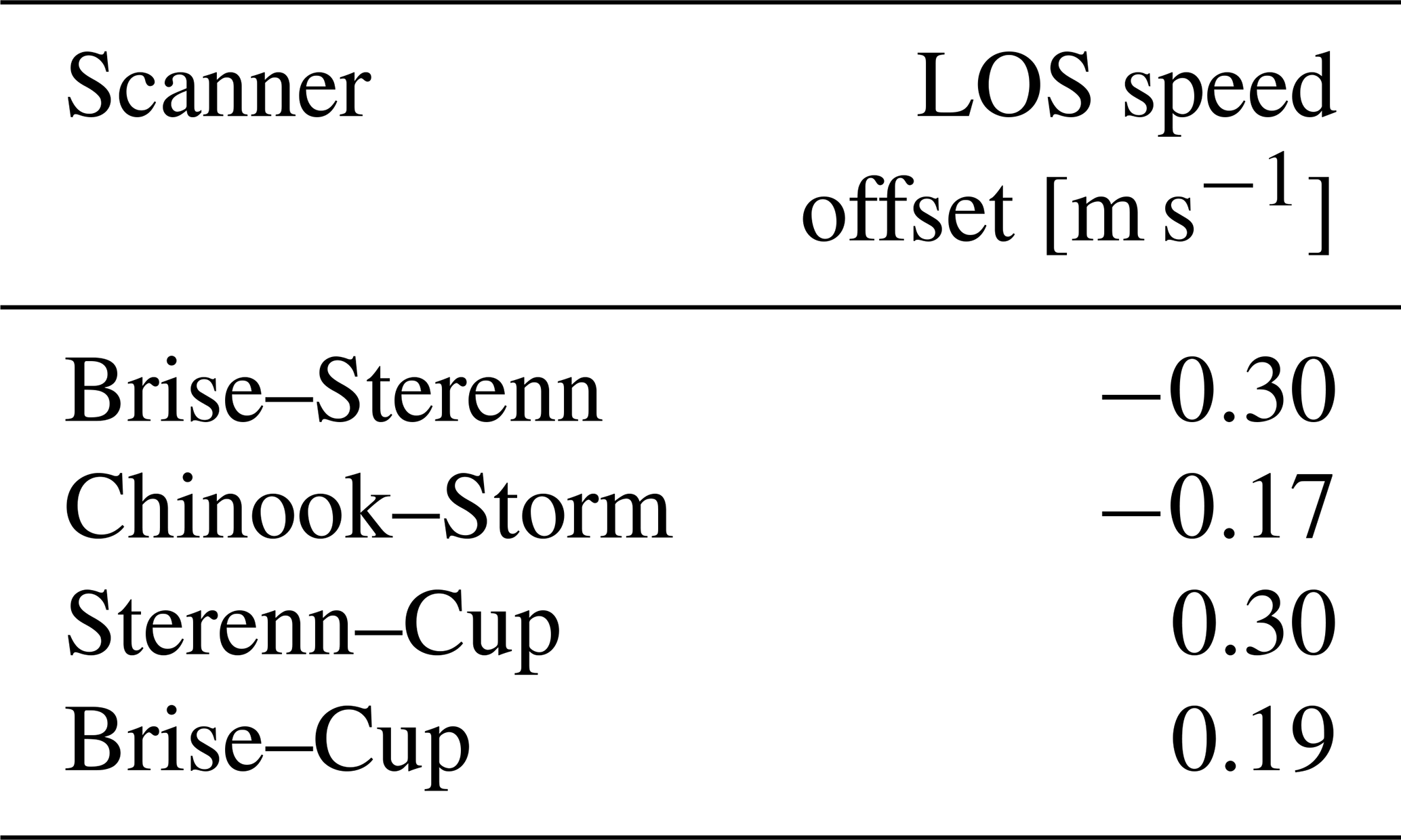
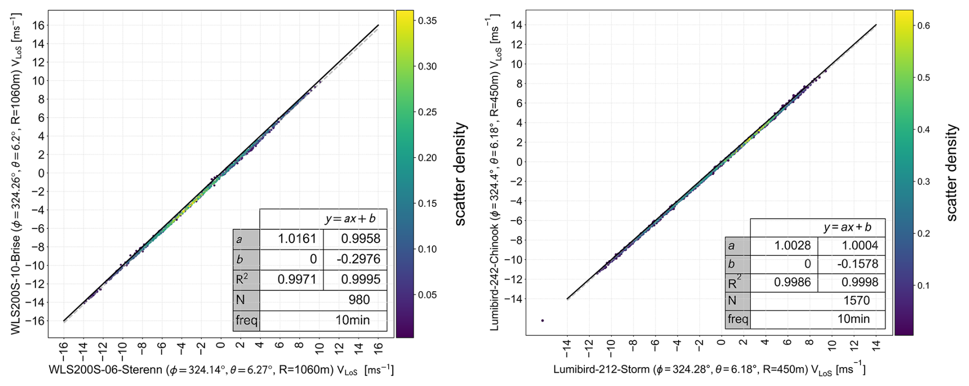
Figure 6 Regression analysis of the two pairs of scanning lidar systems during the pre-calibration test – left: WindScanner system with the range of comparison roughly at the met-mast; right: Streamline/Lumibird system with the range of comparison at 450 m as the met-mast distance could rarely be reached. Results of one- and two-parameter fits are given in the table.

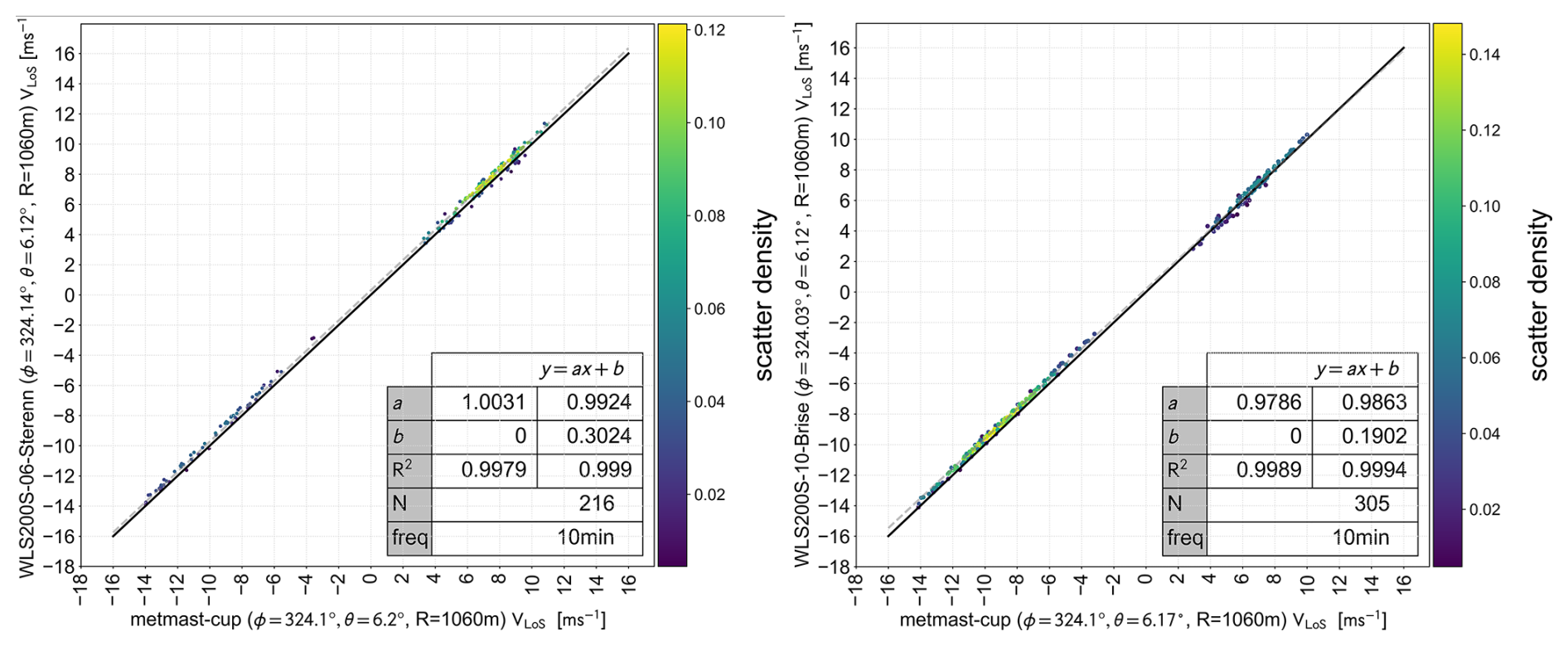
Figure 7 Regression analysis of the scanning lidar systems during the pre-calibration test against the met-mast cup anemometer for the WindScanner systems – left: Sterenn; right: Brise. Only wind direction from ±40° of the line-of-sight direction and corresponding angles of 180° apart have been kept for the analysis. Results of one- and two-parameter fits are given in the table.

2.3.1 Initial hard target mapping

The church and the lighthouse buildings were used as hard targets for aligning the azimuth direction of the scanners at the beginning of the campaign following the procedures of Vasiljević et al. (2016). Each of the hard targets were scanned using stacked sector plan position indicator (PPI) scans with sequential elevation angles, forming a “CNR mapper” as shown in Fig. 8. The elevation and azimuth angle for where the beam is pointing toward the tip of the lighthouse or church roof is determined. The positions of the church and the lighthouse in the global GPS coordinate system were obtained using the DHM (Danish Elevation Model) point cloud, which contains position data collected by laser scanning from an aircraft (see , ). The accuracy in the horizontal and vertical position of each point is given as 0.15 and 0.05 m, respectively; however, given a point density of 8 points m⁻² this gives a point resolution of about 0.35 m (Klimadatastyrelsen, 2025). The distance from the scanner to the church and light hours was about 1600 m. This results in an angular resolution of roughly 0.013°, providing sufficient accuracy for the intended use.

The azimuth offset (ϕ_offset) is calculated as

$$\begin{array}{}\text{(1)}& {\mathit{\varphi }}_{\mathrm{offset}}={\mathit{\varphi }}_{\mathrm{HT}}-{\mathit{\varphi }}_{\mathrm{scanner}},\end{array}$$

where ϕ_HT is the azimuth angle of the pointing direction from the scanner to the hard target in the global coordinate system and ϕ_scanner is the azimuth angle of the pointing direction from the scanner to the hard target in the scanner coordinate system. Note that the azimuth offsets determined via hard-target mapping were not directly implemented as a correction in the lidar software, due to the Lumibird systems not supporting this functionality for all scan types. The azimuth offsets were applied in post-processing, which provided the correct alignment between global and lidar coordinate systems.

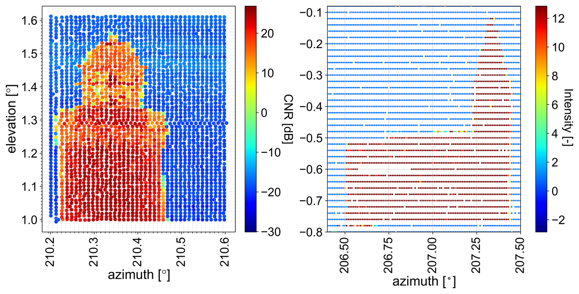
Figure 8 CNR mapper images of the lighthouse (left, Zonda) and church (right, Storm) used to align the beam positions. Stronger return signals appear in red, indicating that the lidar beams intersected a hard target.

Table 4 summarizes the results obtained from the hard target mapping. The initial results from hard-target scanning and wind measurements following deployment of the instruments indicate that the lidar systems were operating normally and were fit for use in the campaign.

Table 4 Results from the hard target mapping performed at the beginning of the campaign.

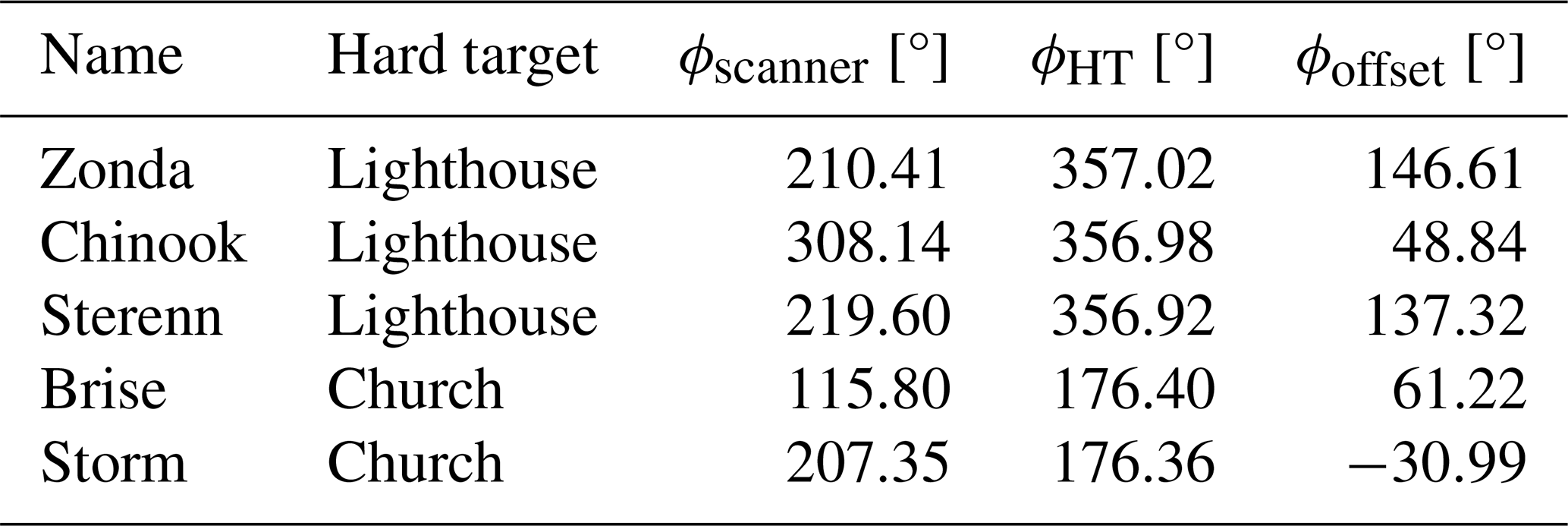
Table 5 Coordinates and height above sea level of the intersection points in experiment phase 1 and 2. The numbers in the first column refer to Fig. 2.

2.3.2 Drone-based pointing verifications

A method for verifying the correct pointing of lidar beams using an aerial drone has been developed by DTU and is described in Thorsen et al. (2023). The drone-based targeting method has the unique advantage of verifying the lidar's pointing accuracy at the actual intended measurement position. Rather than standard hard-target mappings performed at distant positions and generalized across all angles, the drone is flown directly to the desired measurement position which provides a direct verification of the correct positioning of the lidar beam.

The approach involves setting each lidar to stare at its intended measurement position while a drone equipped with a highly accurate real-time kinematic (RTK) positioning system is manually steered into the beam path. The drone is guided using a telescopic sight mounted on top of the scanner head, which is approximately aligned with the lidar beam. This allows the operator to visually steer the drone into the beam. The lidar detects the drone along its beam through the high signal reflectivity indicated by the CNR value, similar to traditional hard target mapping. By combining lidar and drone data, the actual beam position in global coordinates can be determined, allowing either confirmation of correct pointing or quantification of the offsets required to align the beams. To increase the precision of the estimated beam pointing direction, the angular size of the drone should be as small as possible. This can be achieved by increasing the distance between the drone and the scanner or by reducing the physical size of the drone, in this case by adjusting the leg configuration. However, under windy conditions, the drone experiences significant motion, making it difficult to precisely control and to steer it into the narrow lidar beam. As a result, successfully intersecting the beam becomes more challenging. In such conditions, increasing the effective size of the drone improves the likelihood of detection. Additionally, operating closer to the scanner makes steering easier, as the drone appears larger in the telescopic sight, improving visibility and control. Consequently, a trade-off arises between minimizing angular size for precision and increasing it to ensure reliable beam interception under practical conditions. This trade-off influences the achieved accuracy of the estimated beam pointing direction, as reflected in the results presented in Tables 6 and 7.

This exercise was performed twice during the FLOW campaign on all scanning lidars, both at the start and end of the measurements. Beyond obtaining two independent results of the pointing accuracy, repeating the exercise also provides an indication of the consistency of the pointing throughout the measurement period.

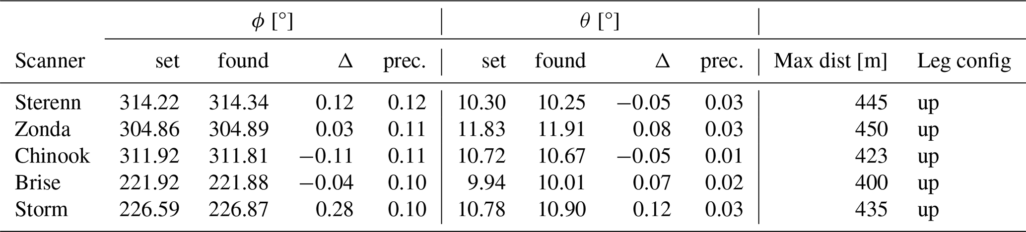
The results of the drone pointing verification are provided in Tables 6 and 7. It should be noted that the values of Δϕ and Δθ are calculated as the estimated pointing direction using the drone (found) minus the desired pointing direction (global). Since the scanner set point angles were changed after the mid-campaign sea surface leveling, the Δθ values obtained for the second drone test reflect the updated angle set points and are therefore expected to be smaller than those obtained before the correction. It should also be noted that due to the correction of the angle set point, the results of the sea surface leveling verification at the end of the campaign can not be directly compared as the sea surface leveling verification only gives the misalignment of the scanner and does not include the correction. To put these results into context, the elevation angle θ difference found using the drone method ranges between −0.2 and 0.15°, which corresponds to a height error in the lidar's beam position of between −3.9 and 3.0 m at intersection point C depicted in Fig. 1. This range of errors is negligible considering the vertical scales of interest in this study.

Table 6 Drone pointing verification results (8 February 2024). For each scanner, ϕ (azimuth angle) and θ (elevation angle) are compared between global reference values (global) and drone-derived estimates (found). Δ denotes the difference (found − global), and prec. represents the estimated measurement precision. Max dist is the maximum drone-to-scanner distance during the test, and Leg config describes the drone leg configuration during the flight.

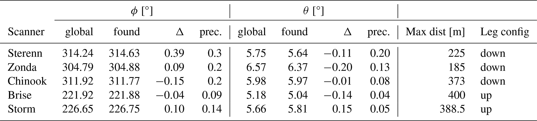
Table 7 Drone pointing verification results (June 25, 2024). For each scanner, ϕ (azimuth) and θ (elevation) set values are compared with drone-derived estimates (found). Δ denotes the difference (found − set), and prec. represents the estimated precision. Max dist is the maximum drone-to-scanner distance, and Leg config describes the flight path configuration. All angles are given in degrees.

2.3.3 Sea surface leveling verification

A further method to independently verify the correct leveling and range reference of the lidars is by scanning the sea-surface (either using PPI or RHI scans). Due to the narrow visibility of the water surface from the lidar positions, we used the RHI scans to determine the distance to the water, r_ss as a function of elevation angle, θ_ss, in this campaign.

The sea surface detection method is based on fitting the carrier-to-noise ratio (CNR) signal as a function of range. In the original approach described by Rott et al. (2022), the CNR–range relationship was fitted using an inverse sigmoid function to identify the inflection point corresponding to the water surface. This approach was later extended by Gramitzky et al. (2024), who combined the sigmoid function with a linear term to account for the gradual decrease in CNR at larger distances. A further refinement was introduced by Gramitzky et al. (2026), who accounted for the logarithmic nature of the CNR signal by introducing an offset to the inflection point, suggested to be approximately half of the probe length.

In the present study, the probe lengths are 25 m for the Windscanner and WindCube systems and 12 m for the Streamline systems, which are significantly shorter than the 75 m probe length considered by Gramitzky et al. (2026). That study also demonstrated that large start or stop elevation angles can introduce significant errors in the estimated elevation. In this campaign, however, the scanner placement near a coastal bluff restricted the usable elevation range to approximately 1.5°. Combined with the expectation of small tilt and elevation offsets – due to prior alignment – this suggests that the influence of the range offset is limited.

To verify this assumption, the analysis was repeated using offsets of −6 m for the Streamline systems and −12.5 m for the Windscanner and WindCube systems. These offsets deviate slightly from the recommendation in Gramitzky et al. (2026) but resulted in only minor differences of approximately 0.01–0.02° in the estimated elevation error, which is negligible for the purposes of this study. Therefore the result in Table 8 does not use the range offset as suggested by Gramitzky et al. (2026).

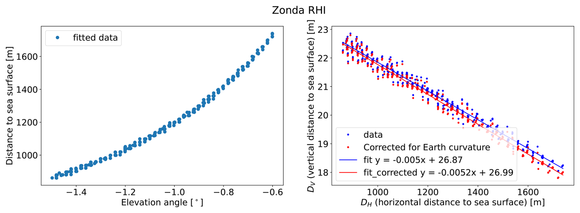
A vertical cross section of the land, sea, and sky was scanned by each lidar. The curve of signal reflectivity (CNR) across distance inflects at the elevation position corresponding to the water surface, as depicted in Fig. 9, which shows a single example from Chinook where the water surface was found at 1000 m for the corresponding elevation angle. Using this principle with multiple RHI scans repeated at the same azimuth angle provides a linear fit result such as the one shown in Fig. 10 for Zonda. Here, the vertical and horizontal distances, from the scanner head to the sea surface, D_v and D_h, are calculated as

$$\begin{array}{}\text{(2)}& {\displaystyle }{D}_{\mathrm{v}}=r_{\mathrm{ss}}\sin {\mathit{\theta }}_{\mathrm{ss}},\text{(3)}& {\displaystyle }{D}_{\mathrm{h}}=r_{\mathrm{ss}}\cos {\mathit{\theta }}_{\mathrm{ss}},\end{array}$$

For the longer ranges used here, it is also necessary to correct for the effect of the curvature of the Earth. Here the vertical distance is corrected by Δh, which for horizontal distances much smaller than the radius of the earth, r_earth, is written as

$$\begin{array}{}\text{(4)}& {\displaystyle }\mathrm{\Delta }h=r_{\mathrm{earth}}\left(\mathrm{1}-\cos \left({\displaystyle \frac{D_{\mathrm{h}}}{r_{\mathrm{earth}}}}\right)\right).\end{array}$$

The elevation error in the scanner in radians is given as the slope of the linear fit shown in Fig. 10. It is possible to further extend this method across multiple azimuth positions to obtain tilt, roll, and range offset results for each lidar; however, it was not necessary to do so in this campaign due to the configuration of the lidars being used to stare at a single position. The sea surface leveling exercise was repeated twice during the campaign. The results from the two sea surface leveling exercises are shown in Table 8. In the results from April 2024, the elevation error found on Zonda was so large that it was decided to correct the elevation angle of the lidar in phase 2 of the experiment, using the results from April 2024 listed in Table 8.

Table 8 Results from the sea surface RHI scans.

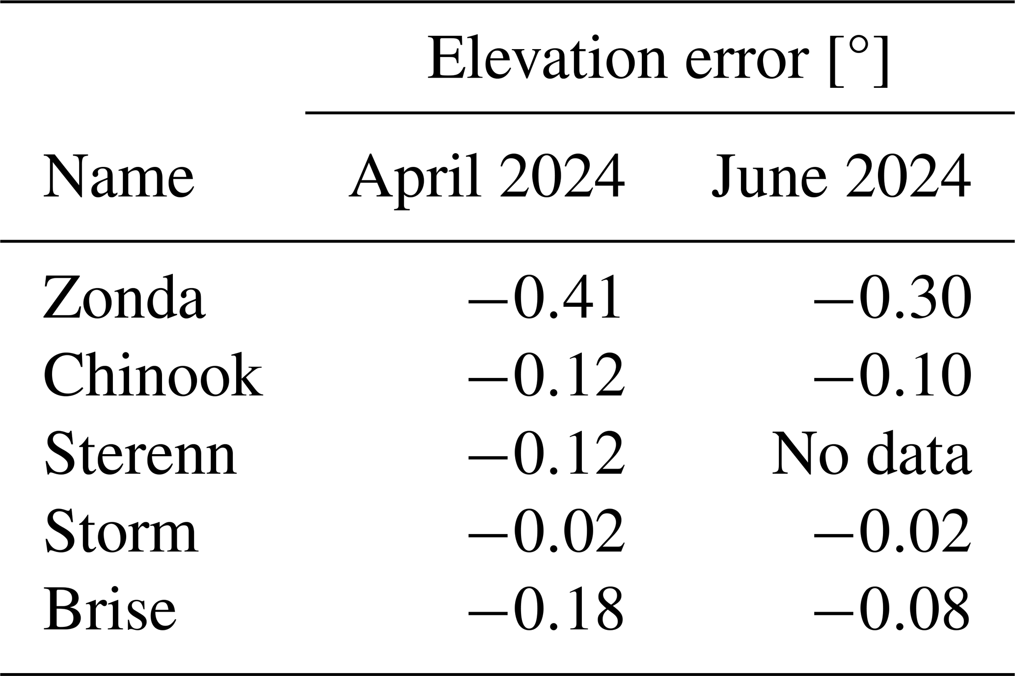
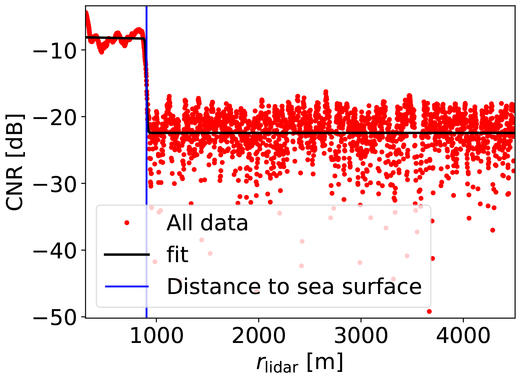
Figure 9 Single SSL measurement point from Chinook, showing the CNR value as a function of distance where the water surface is identified at 1000 m for the corresponding elevation angle.

Figure 10 Results from repeated SSL RHI scans from Zonda at a single azimuth position. The distance to the sea surface was found using the method shown in Fig. 9.

2.3.4 Post-campaign LOS speed inter-comparison and offset verification

The final quality control effort took place at the end of the field campaign, which evaluated each lidar's line-of-sight speed offset, and the relative LOS speeds measured by lidars at the same deployment site. This test would demonstrate either that the systems were measuring the correct speeds consistent with the pre-campaign test results or that an issue had occurred which would require a correction to the lidar data.

This exercise involved grouping the systems by deployment location (i.e.,  church vs. lighthouse), and performing an inter-comparison of measured LOS speeds between lidar pairs at the same site. This was done by placing the beams of all lidars at each site in parallel and evaluating the independent observations of LOS speeds between all possible pairs of lidars at each location. Since the lidars were deployed next to each other and had their beams aligned in parallel, the measured values should be nearly identical. An important limitation of this approach is that since the two lidar groups are separated, it is not possible to make a meaningful comparison between lidars across the two sites. The high-frequency data were filtered and averaged into 10 min intervals. For the Windscanner and WindCube systems, all LOS samples with a CNR ≤−22 dB or with retrieved LOS wind speeds outside the interval [−40, 40] m s⁻¹ were removed. For the StreamLine XR+ systems, all LOS samples with signal intensity ≤1.009 dB or with retrieved LOS wind speeds outside the same interval were discarded. Furthermore, 10 min intervals containing fewer than 1000 valid samples after filtering were excluded. Following this data cleaning procedure, the data were binned in 1 m s⁻¹ increments (see red points in Fig. 11). Applying a linear regression between binned observations of the lidar pairs provides a coefficient, offset, and fit indicator of the agreement between the lidars. Figure 11 shows the LOS speed comparison between Brise and Storm for a single range, which is then extended across multiple ranges in Fig. 12. Since the offset was expected to change significantly over 100 m, the results were only calculated every 100 m.

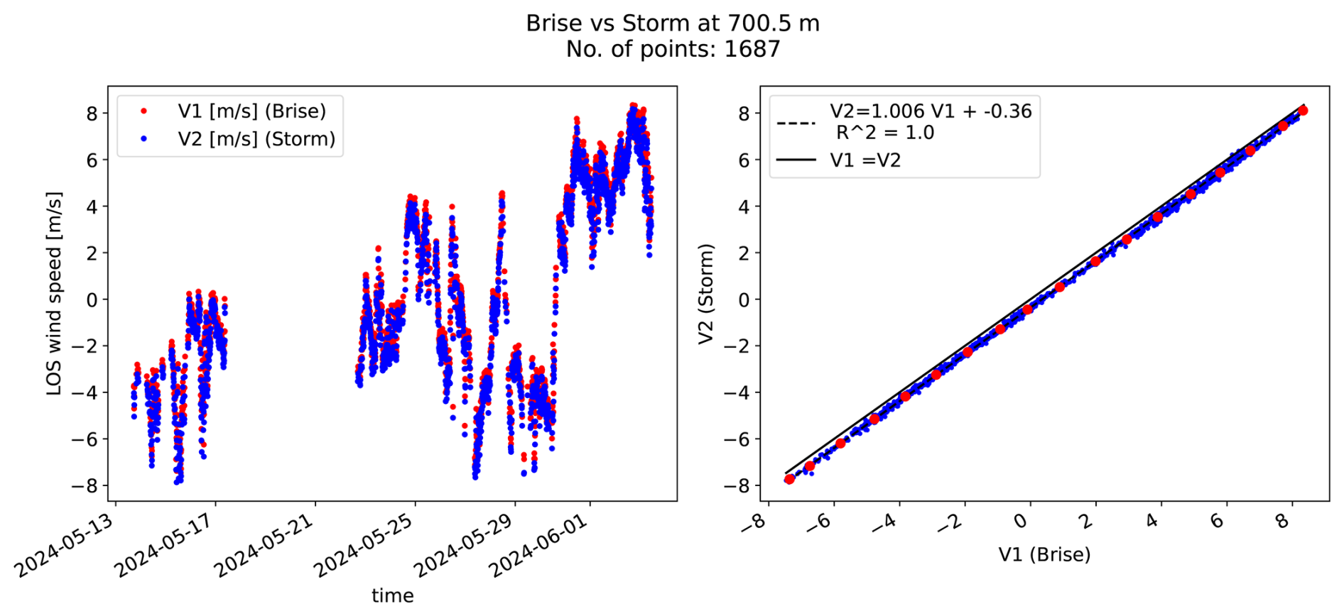
Figure 11 Post-campaign LOS speed inter-comparison between Brise and Storm at 700.5 m range. Time series (left) and binned linear regression (right, units on the axes are in m s⁻¹) with fit parameters.

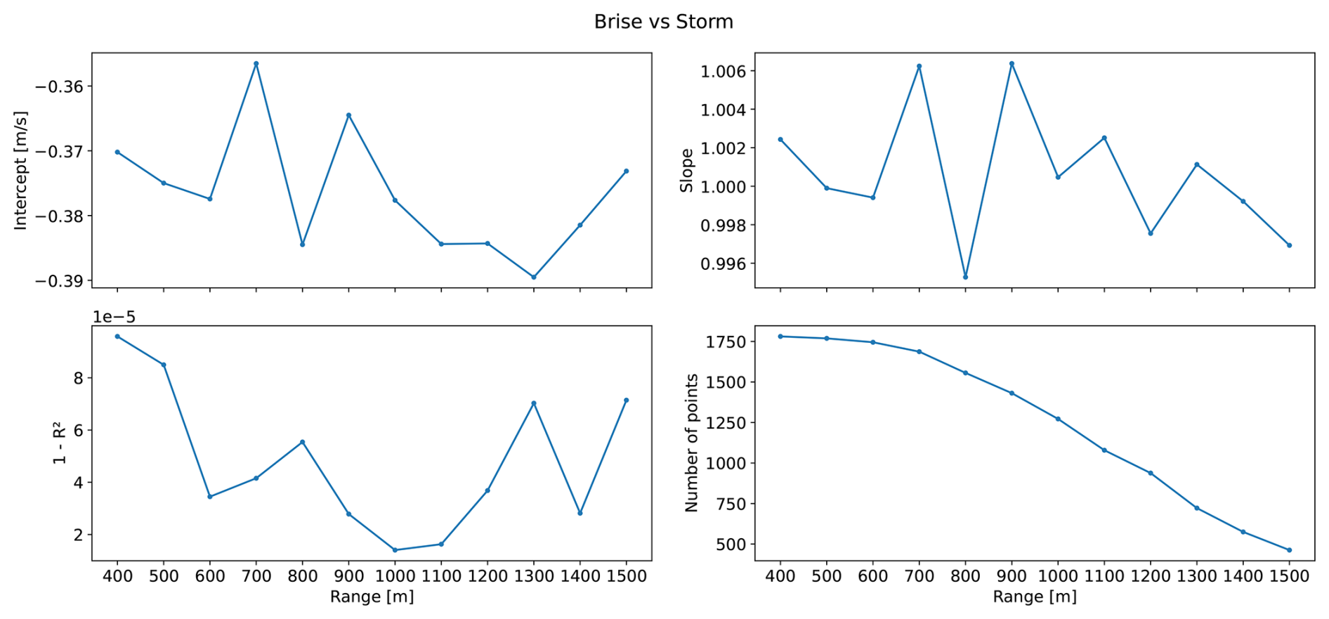
Figure 12 Linear fit parameters of post-campaign LOS speed inter-comparison between Brise and Storm across all ranges indicating good agreement between the two systems.

Table 9 Results from the post-campaign line-of-sight speed comparison between lidars at each site.

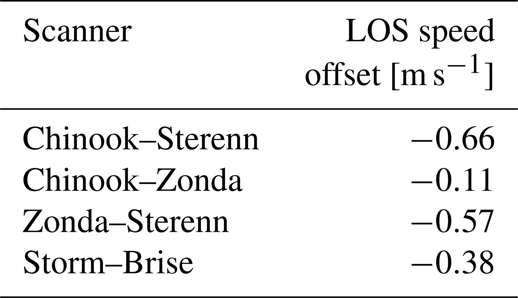
Table 10 Final, recommended velocities to be added to the line-of-sight velocities for each lidar.

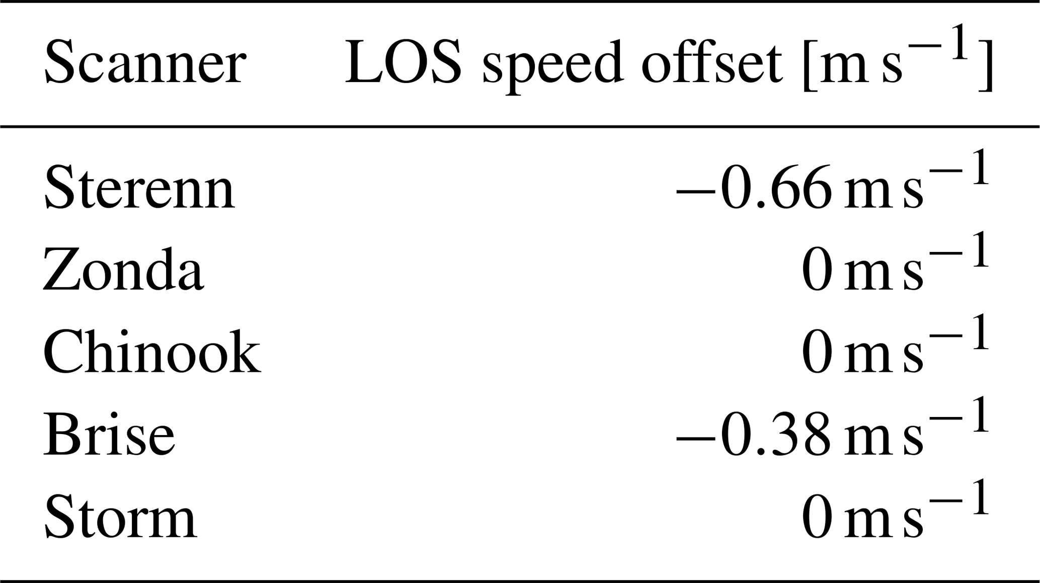
From the linear regression the offsets are averaged over all distances and shown in Table 9. The comparison involving Brise and Sterenn shows a significant offset compared to the comparison between Chinook and Zonda. The StreamLine units were sent to the factory for repair prior to the campaign, where they were tested against a reference lidar. These tests showed that the StreamLine units (Chinook and Storm) did not exhibit any significant LOS speed offsets. Considering this, the offsets identified in the post-campaign LOS speed calibration are primarily attributed to Brise and Sterenn, with magnitudes of approximately −0.4 m s⁻¹ for Brise and −0.7 m s⁻¹ for Sterenn. When compared with the pre-campaign test results, the findings are consistent in the sense that Sterenn shows a larger offset than Brise. Both offsets are substantial and should be corrected for during data analysis. A smaller offset of about 0.1 m s⁻¹ is observed between Zonda and Chinook, but because the data will be used for turbulence analysis, this discrepancy is less critical. The final, recommended offsets are shown in Table 10.

3 Data description

This section describes what is contained in the publicly available data repository (Patel et al., 2025). The following variables are present in the dataset.

1. Radial velocity: the measured wind speed along the lidar beam in m s⁻¹. It is measured at a frequency of 2 Hz (except for Zonda which measured at 1 Hz). Moreover, the radial velocity measurements are taken at multiple points along the lidar beam. These points are commonly referred to as range gates. Table 2 provides information on the range gates of each lidar.

2. Quantification of noise: the definition of noise in the radial velocity measurement differs for the five lidars. In the case of Zonda, Sterenn, and Brise (see Table 2), it is quantified using the signal-to-noise ratio (SNR) expressed in decibels. On the other hand, the noise in Chinook and Storm is quantified using Streamline intensity (s), which can be related to the SNR as follows:

   $$\begin{array}{}\text{(5)}& \text{SNR}=\mathrm{10}{\log }_{\mathrm{10}}(s-\mathrm{1})\mathrm{dB}.\end{array}$$

   Note that both SNR and s are measured at all range gates and at the same frequency as the radial velocity measurements.

3. Ceilometer data: the ceilometer data contain the aerosol backscatter signal sampled every 16 s and at a vertical resolution of 10 m. We refer the reader to Vaisala's technical documentation of the CL31 ceilometer for a more in-depth description of the other data available from this device (, ).

Note that the dataset covers the entire period of the campaign from February 2024 to June 2024 while the periods corresponding to intra-campaign calibration (see Fig. 4) are not included. Thus, the data can be read by selecting the required time period and the range gate. We recommend using the scripts provided at https://data.dtu.dk/articles/dataset/Trans_experiment_data_paper_script/29224631 (last access: 20 August 2026). Moreover, offsets of −0.66 and −0.38 m s⁻¹ must be added to the data from Sterenn and Brise, respectively.

4 Quality control of the campaign dataset

This section presents the post-processing of the raw lidar data in order to describe its quality. Note that the offsets shown in Table 10 were added to the data after reading from the raw dataset. We first define a filtering criterion to separate good and bad data. The latter is a result of many spikes being present in the time series due to low concentration of aerosols in the atmosphere, dirt on the lens, presence of obstacles in the lidar beam, etc (Vasiljević et al., 2016). The complete removal of noisy data, that is, the full 10 min period, is necessary when analyzing turbulence spectra or coherence because noise removal algorithms might introduce too many gaps (Beck and Kühn, 2017). In the literature, noise is often characterized by the signal-to-noise ratio (SNR) and a flat threshold is applied to it to differentiate between reliable and unreliable data. But the so-called SNR filter suffers from many drawbacks, the most important one being the dependence of the optimal SNR threshold on the site conditions, instrument manufacturer, and experimental setup (Gryning et al., 2016). Indeed, we observed that the SNR threshold varied significantly with the atmospheric conditions. Thus, we choose to characterize the noise by another metric, the standard deviation of the radial velocities calculated over 10 min: ${\mathit{\sigma }}_{v_{\mathrm{r}}}$. We found that it is easier to establish the optimal threshold for ${\mathit{\sigma }}_{v_{\mathrm{r}}}$ as it is mostly independent of the aforementioned factors.

After careful analysis of the data, we concluded that when ${\mathit{\sigma }}_{v_{\mathrm{r}}}$ is greater than 4 m s⁻¹, the 10 min period contains too many spikes. This threshold was determined by analyzing many 10 min time series from the five lidars. Consequently, the corresponding 10 min periods were rejected. On the other hand, when ${\mathit{\sigma }}_{v_{\mathrm{r}}}$ is less than 1.2–1.5 m s⁻¹, depending on the lidar model, the 10 min period is free from spikes. And for those 10 min periods where ${\mathit{\sigma }}_{v_{\mathrm{r}}}$ is between 1.5 and 4 m s⁻¹, it is possible to remove spikes using a de-spiking algorithm such as the one described by Beck and Kühn (2017) without introducing too many gaps. As an example, we show time series from all five lidars in Fig. 13. The data on the right-hand side have many spikes with ${\mathit{\sigma }}_{v_{\mathrm{r}}}$ being greater than 4 m s⁻¹, while the data on the left-hand side are relatively free from noise and ${\mathit{\sigma }}_{v_{\mathrm{r}}}$ is lower than 1.2 m s⁻¹. The de-spiking algorithm developed by Beck and Kühn (2017) uses two-dimensional kernel density estimation (KDE) to find “data-dense” regions which are assumed to be free from noise. We used a modified version of the KDE filter to estimate the distribution of Δv_r instead of v_r, where

$$\begin{array}{}\text{(6)}& \mathrm{\Delta }{v}_{\mathrm{r}}^t=v_{\mathrm{r}}^t-v_{\mathrm{r}}^{t-\mathrm{1}},\end{array}$$

and t represents the indexing of different samples in time.

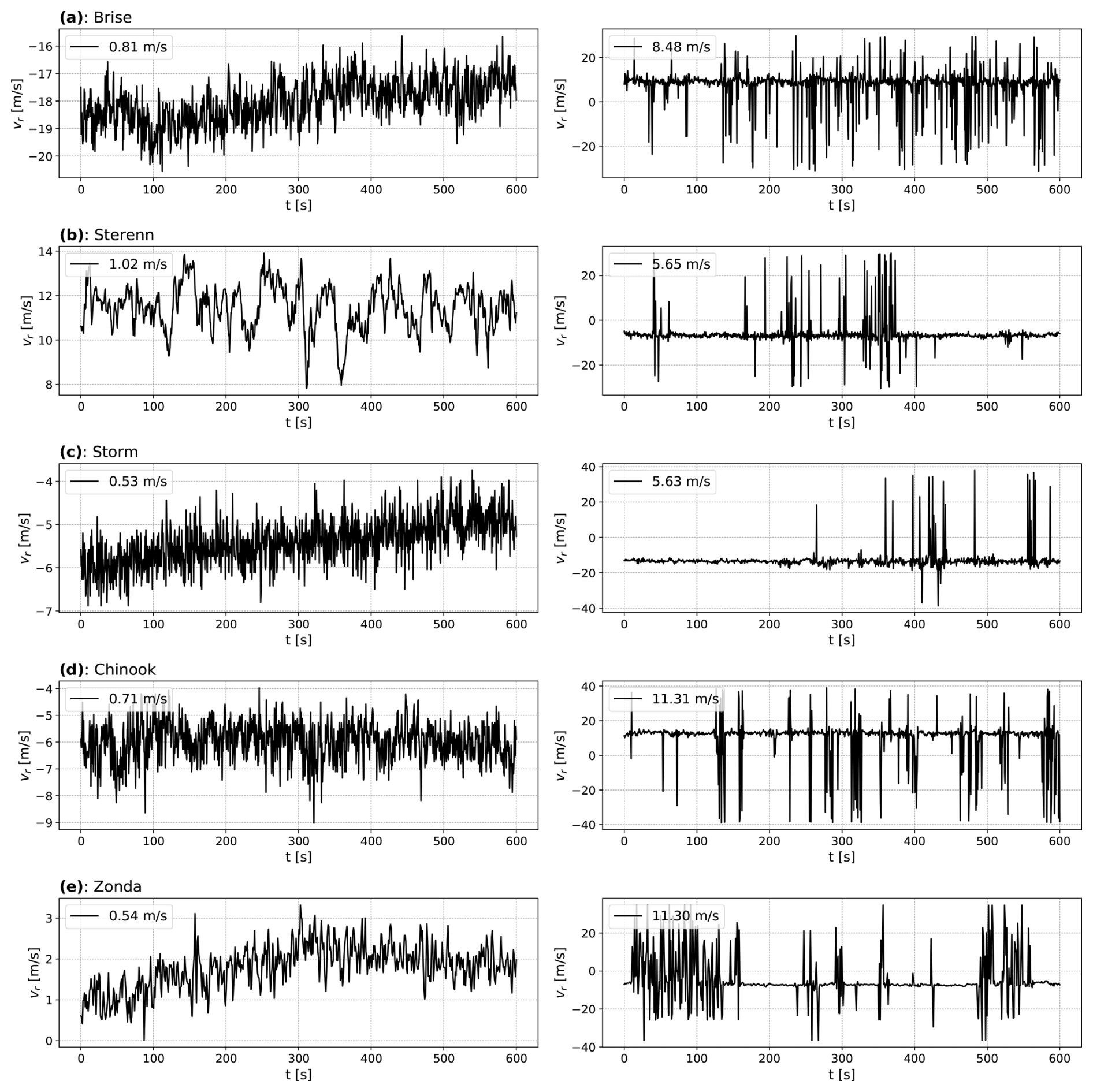
Figure 13 Some 10 min time series from all five lidars showing periods with good data (left) and bad data (right) characterized by ${\mathit{\sigma }}_{v_{\mathrm{r}}}$.

Next, we reconstructed the east–west (v_EW) and north–south (v_NS) wind components at the six crossing points using the following relations (Peña and Mann, 2019):

$$\begin{array}{}\text{(7)}& \underset{{\mathit{v}}_{\mathrm{r}}}{\underbrace{\left[\begin{array}{l}{v}_{r_{\mathrm{1}}}\\ v_{r_{\mathrm{2}}}\end{array}\right]}}=\underset{\mathbf{M}}{\underbrace{\left[\begin{array}{cc}\cos {\mathit{\varphi }}_{\mathrm{1}}\cos {\mathit{\psi }}_{\mathrm{1}}& \sin {\mathit{\varphi }}_{\mathrm{1}}\cos {\mathit{\psi }}_{\mathrm{1}}\\ \cos {\mathit{\varphi }}_{\mathrm{2}}\cos {\mathit{\psi }}_{\mathrm{2}}& \sin {\mathit{\varphi }}_{\mathrm{2}}\cos {\mathit{\psi }}_{\mathrm{2}}\end{array}\right]}}\underset{\mathit{v}}{\underbrace{\left[\begin{array}{l}{v}_{\mathrm{EW}}\\ v_{\mathrm{NS}}\end{array}\right]}},\end{array}$$

and

$$\begin{array}{}\text{(8)}& \mathit{v}={\mathbf{M}}^{-\mathrm{1}}{\mathit{v}}_{\mathrm{r}}.\end{array}$$

The subscripts 1 and 2 refer to the lidars close to the church and lighthouse, respectively, whereas ϕ is the azimuthal orientation of the beam and ψ is its elevation. Equation (7) relies on the assumption that the projection of the vertical wind component along the lidar beam is negligible. Given the small elevation angles of the beams, this assumption is justified. Since the beams of the church and lighthouse lidars are approximately 90° apart, when using Eqs. (7) and (8), the uncertainty becomes almost independent of the wind direction (Peña and Mann, 2019). However, Eq. (7) implicitly introduces another filter criterion: data from two lidars must be available simultaneously. Data availability after applying the ${\mathit{\sigma }}_{v_{\mathrm{r}}}$ and modified KDE filters is not uniform across the five lidars. Some lidars provided noisier data than the rest, probably because they were older models (Sterenn) or had accumulated more dirt on the lens (Chinook). This can be seen in Fig. 14 where Storm, Zonda, and Brise have many more 10 min periods with ${\mathit{\sigma }}_{v_{\mathrm{r}}}$ between 0 to 2 m s⁻¹. Thus, the data availability is lowered when reconstructing the true wind vector, especially at crossing points with Sterenn and Chinook. This lidar pair has a joint availability of 17 % while Zonda and Storm has the highest joint availability of 50 %.

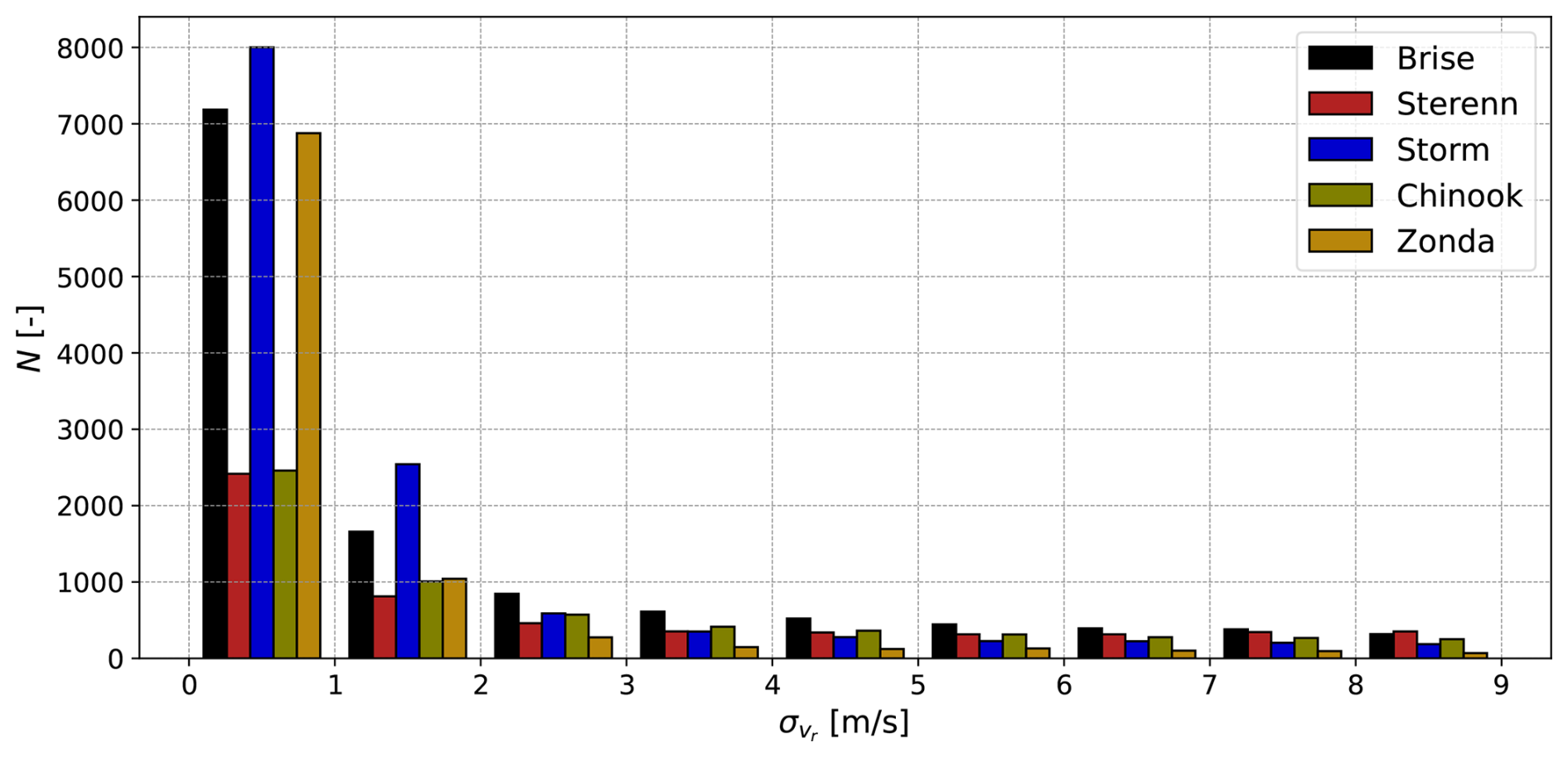
Figure 14 Histogram of ${\mathit{\sigma }}_{v_{\mathrm{r}}}$ for the five lidars using data from one of the range gates present at the intersection points.

Subsequently, we computed the instantaneous horizontal wind speed, u_hor:

$$\begin{array}{}\text{(9)}& u_{\mathrm{hor}}=\sqrt{v_{\mathrm{EW}}^{\mathrm{2}}+v_{\mathrm{NS}}^{\mathrm{2}}},\end{array}$$

and the wind direction, θ:

$$\begin{array}{}\text{(10)}& \mathit{\theta }=\arctan \left(-v_{\mathrm{EW}},-v_{\mathrm{NS}}\right).\end{array}$$

Note that this wind direction is expressed in the meteorological convention, where 0° is aligned with true north and increases in the clockwise sense, and that the first argument in the arctan function is “y” (“opposite”). The histograms of the 10 min mean horizontal wind speed (U_hor) and wind direction (Θ) are shown in Figs. 15 and 16, respectively. The modal 10 min wind speed is between 11 and 12 m s⁻¹ and the maximum observed value of U_hor was 26.2 m s⁻¹. The modal wind direction was between 210 to 220° from the start of the campaign to the end of April 2024, while from May 2024 to the end of the campaign, it was between 290 and 300°. This corresponds to westerly circulation over the northern mid-latitudes due to the Ferrel cell. Easterly winds are also frequently observed, but the data are affected by the terrain.

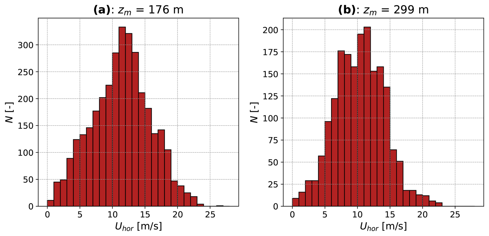
Figure 15 Histogram of the 10 min mean wind speed at point 2 in beam direction 1 (a) and 2 (b).

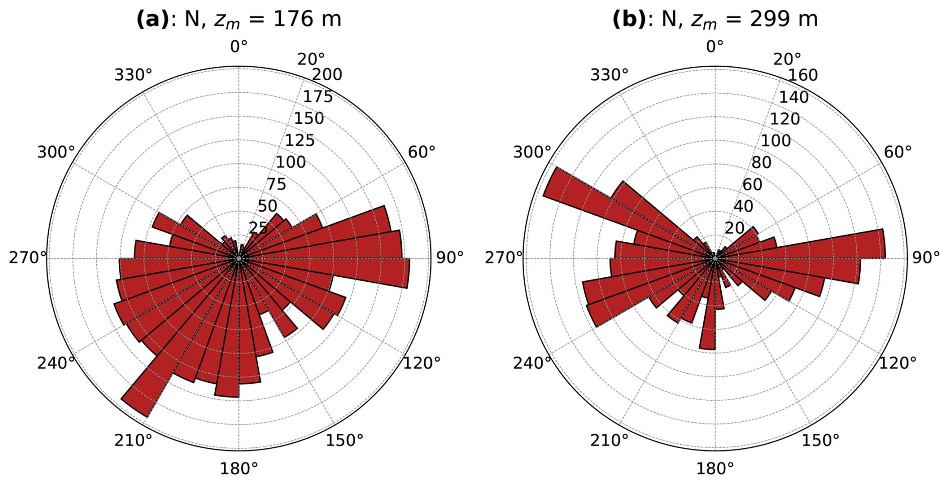
Figure 16 Histogram of the 10 min mean wind direction in polar coordinates at point 2 in beam direction 1 (a) and 2 (b).

We also present an example of how the data can be used to compute the turbulence spectra and coherence, which are displayed in Fig. 17. Note that a detailed analysis of these is presented in Patel et al. (2026) wherein the effect of the systematic biases of the lidar are also given an in-depth treatment.

We compute the spectra from N_k time series that are each 20 min long in duration. First the coordinate system is changed such that the x axis is aligned with the mean wind direction over 20 min:

$$\begin{array}{}\text{(11)}& {\displaystyle }u=u_{\mathrm{hor}}\cos \left(\mathit{\theta }-\mathrm{\Theta }\right),\text{(12)}& {\displaystyle }v=u_{\mathrm{hor}}\sin \left(\mathit{\theta }-\mathrm{\Theta }\right),\end{array}$$

where u is the along-wind component, v is the cross-wind component, and Θ is the mean wind direction. Then, the auto-spectrum is calculated by Lumley (1970):

$$\begin{array}{}\text{(13)}& S_i\left(f\right)={\displaystyle \frac{\mathrm{2}\mathit{\pi }}{N_{k}T}}\sum _{k=\mathrm{1}}^{N_k}{\left|{\mathrm{u}}_i^k\left(f,T\right)\right|}^{\mathrm{2}},\end{array}$$

where

$$\begin{array}{}\text{(14)}& {\mathrm{u}}_i^k\left(f,T\right)={\displaystyle \frac{\mathrm{1}}{\mathrm{2}\mathit{\pi }}}\underset{\mathrm{0}}{\overset{T}{\int }}{u}_i^k\left(t\right)\exp (-\mathrm{2}\mathit{\pi }ift)\mathrm{d}t\end{array}$$

is the Fourier transform of each individual time series of length T=1200 s. Moreover, u₁=u and u₂=v. In the example shown here, N_k=6.

In order to find the lateral coherence, we use concurrent time series of radial velocities from the lidars Zonda and Brise to reconstruct the horizontal wind components at intersection point number 1 and radial velocities from Sterenn and Storm for intersection point number 4. Note that they are horizontally separated by 224 m and vertically by 8 m. First, the cross-spectrum is calculated via

$$\begin{array}{}\text{(15)}& {\mathit{\chi }}_{ij}\left(f,{\mathrm{\Delta }}_y,{\mathrm{\Delta }}_z\right)={\displaystyle \frac{\mathrm{2}\mathit{\pi }}{N_{k}T}}\sum _{k=\mathrm{1}}^N{\mathrm{u}}_i^k\left(f,T,\mathrm{0},\mathrm{0}\right){\mathrm{u}}_j^{k*}\left(f,T,{\mathrm{\Delta }}_y,{\mathrm{\Delta }}_z\right),\end{array}$$

where $(\cdot {)}^{*}$ indicates complex conjugation. Then, the root-coherence is given by

$$\begin{array}{}\text{(16)}& {\mathit{\gamma }}_{ij}\left(f,{\mathrm{\Delta }}_y,{\mathrm{\Delta }}_z\right)={\displaystyle \frac{\mathrm{\Re }\left({\mathit{\chi }}_{ij}\left(f,{\mathrm{\Delta }}_y,{\mathrm{\Delta }}_z\right)\right)}{\sqrt{F_i\left(f\right)F_j\left(f\right)}}},\end{array}$$

where ℜ(⋅) refers to the real part of the complex cross-spectrum.

The spectra and coherence show a strong dependence on atmospheric stability and in many cases, mesoscale turbulence causes an increase in energy at the low-frequency end. These effects are discussed in depth in Patel et al. (2026) wherein the measurements are also compared to the model of Mann (1994) and Syed and Mann (2024).

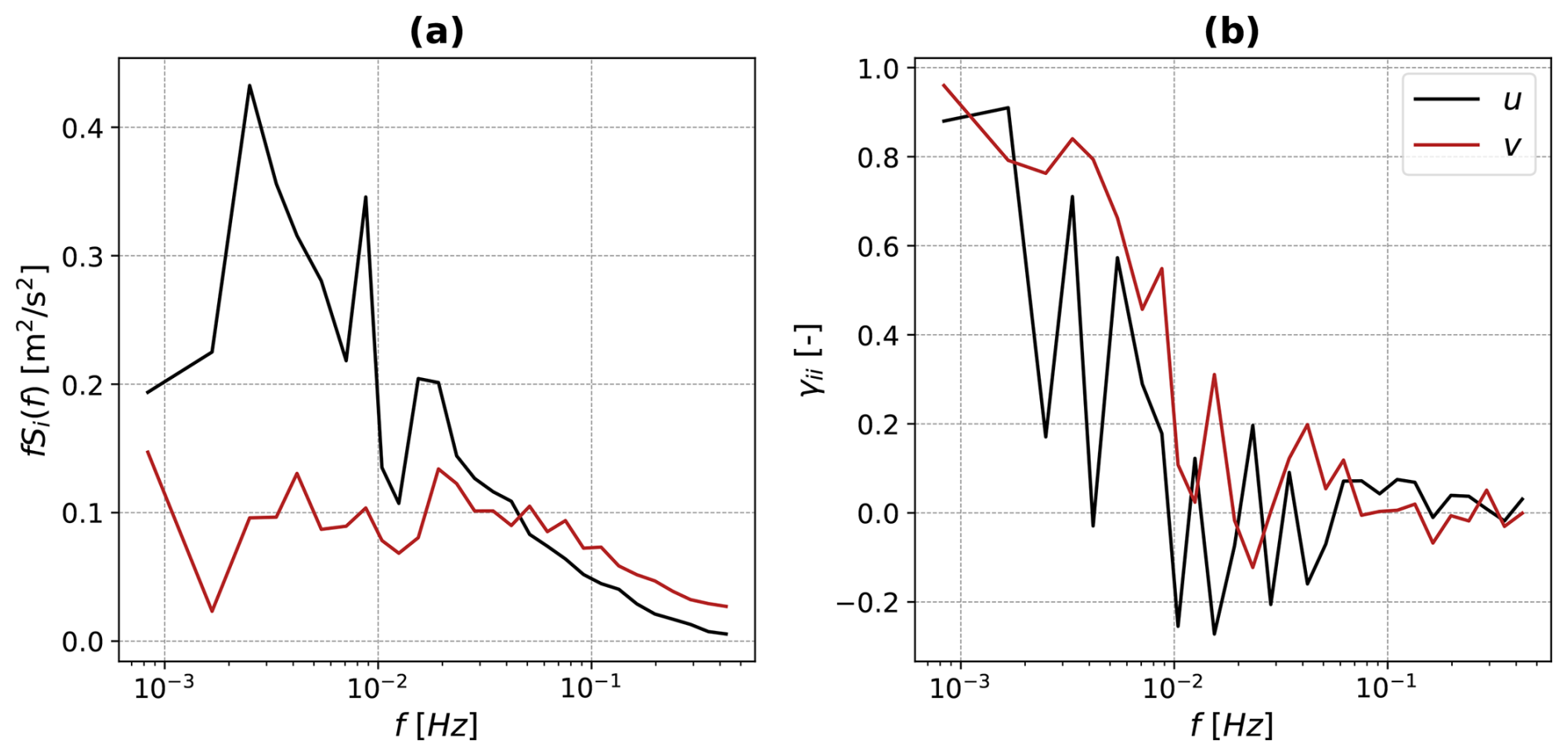
Figure 17 An example of auto-spectra (a) and lateral coherence (b) calculated from the lidar measurements over a period of 2 h with a mean wind speed of 17.9 m s⁻¹, mean wind direction of 296°, and at a height of 159 m. The separation for the coherence estimation is Δy=224 m and Δz=8 m.

5 Conclusions

A measurement campaign that recorded the horizontal wind components at 150 to 250 m above the sea was presented. The experiment used five lidars placed along the west coast of Denmark, with their beams intersecting in a close-to-horizontal plane. This allowed the wind data to be measured concurrently at six different points from which the lateral coherence could be computed. The lidars were calibrated before, during, and after the experiment via a few different methods which included the usage of drones, sea-surface leveling, and hard target mapping. We also described the storage format of the data and how they can be retrieved for further analysis. Quality checks on the lidar data showed that two instruments suffered from poor signal quality, which lowered the data availability at the respective intersection points. The 10 min statistics of the wind speed and direction followed the trends expected at the geographic location of the site. We show an example to illustrate how the measurements can be used to analyze auto-spectra and lateral coherence at heights relevant for offshore wind turbines and validate newer turbulence models, as shown in Patel et al. (2026). The dataset could also be used to study wind profiles and gusts in the MBL.