Modelling of wind flows over realistic forests with LES

A large-eddy simulation (LES)-based model for the representation of wind flows over realistic forests and topography is presented. Terrain elevation and forest density maps from airborne laser scans are employed to investigate the importance of specific model choices related to capturing upstream terrain effects on the wind resource. The study is divided into three parts. Firstly, an extended verification process under idealized conditions is carried out. Secondly, a validation is done where the model is compared to field measurements acquired in the southeast of Sweden, and, finally, an assessment of the forest and terrain footprint is carried out based on variations in the surface representation. The results show agreement of turbulence statistics compared to the literature when the forest is explicitly modelled, following expected trends as a function of the tree density. When the forest is explicitly modelled, the impact of the ground roughness becomes insignificant, even for an unrealistically sparse forest. The study also demonstrates that a model relying only on ground roughness yields notable differences in the turbulence characteristics. This is partly attributed to the inability of the model to reproduce sufficient drag for forest-equivalent values of roughness length z₀ while maintaining the applicability of wall functions, which can impose strict limitations on the grid near the ground. This is further complicated by the problem of converting realistic, heterogeneous forest fields to z₀. Moreover, turbulence statistics in the roughness sublayer are affected by the lack of vertical permeability. The validation shows that the model is able to capture the flow characteristics imprinted by different surface features on the wind along three distinctive wind directions. Vertically separated spectral coherence from the LES is slightly below that of the IEC standard, which can be attributed to the reference velocities used in the normalization of the frequency. The footprint study shows that the heterogeneity of a realistic forest produces higher drag in comparison with homogeneous conditions while also providing better agreement with observations. An analysis based on correlations of upstream forest drag with target wind statistics shows that a point above the terrain is most significantly influenced by the footprint of a forest area located at about 10 times upstream of its height above ground. When correlations are applied to turbulence, this separation increases five-fold. These findings provide valuable insight to determine the optimal domain size of a computational domain in forest simulations under neutral atmospheric stratification. Further comparisons of fully uniform vs. limited areas of realistic forest revealed that at heights above 100 m, no clear differences in the wind flow are seen. Conversely, comparing flat terrain with the actual topography – with a realistic forest distribution in both cases – demonstrated the clear importance of capturing small-scale terrain features.

1 Introduction

The expansion of wind energy has led to an increasing interest in the development of projects over remote locations that offer conditions far from the flat and obstacle-free surface considered ideal. Forested regions are of interest due to reasons such as reduced social opposition and concurrent interests with the forestry sector in sharing costs for access roads and management. Conversely, they present some of the most challenging wind conditions for the operation of wind turbines: the wind speed is lower, with a stronger vertical shear and higher turbulence intensity compared to winds over terrain with lower vegetation. Indeed, in forested locations, wind turbines require more maintenance (Zendehbad et al., 2016). The study of wind flows above forests is far from being restricted to the wind energy community; on the contrary, it is highly relevant in investigations concerning any other structure found on such regions that is subjected to large dynamic loads, such as buildings or bridges, as well as decidedly important in forestry and agricultural applications (Niklas, 1985; Gardiner, 1994; Schindler et al., 2012).

Wind flow over forested terrains differs in some aspects compared to that over terrains free of vegetation. The former carries large coherent structures that penetrate the canopy and dominate the turbulence dynamics, including momentum fluxes and scalar transport. In some aspects the description of a canopy flow fits more with that of a mixing layer than a boundary layer, an analogy first made by Raupach et al. (1996). This is revealed by the distinctive inflection point in the velocity profile at the canopy top and other contrasting features to those of a surface layer flow, such as variations in high-order statistical moments, the growth pattern of the turbulence lengthscales, or the relations between sweeps and ejections, defined by the directions of the components of shear stress (Gardiner, 1994). The main characteristics of canopy turbulence, gathered from experimental field campaigns and wind tunnel data, were depicted by Raupach et al. (1996) in figures they called a “family portrait”, providing a quick reference for the turbulence characteristics for varying canopy heights and densities. These figures have since been reproduced and complemented by other authors, for instance, Brunet (2020). The effect of the forest in this roughness sublayer is conventionally assumed to extend vertically to $z\approx \mathrm{2}\sim \mathrm{3}$ times the forest height h. Above it, the wind profile recovers its near-logarithmic shape with height z−d, where d is the zero plane displacement height, identified by Thom (1971) and later Jackson (1981) as the level at which the mean drag appears to act on the flow. The asymptotic transition to turbulence statistics similar to those over low vegetation at $z\approx \mathrm{2}\sim \mathrm{3}h$ is also supported by measurements over real forests (Arnqvist et al., 2015, 2024).

A relevant problem when modelling flows over high roughness at high resolution is that the first grid node above ground ends up embedded deep within the roughness sublayer, where usual flux–gradient expressions are invalid (Basu and Lacser, 2017). Since the roughness sublayer is estimated to be two to three tree heights deep, this problem will be present for microscale simulations of all natural forests. While solutions do exist, they come with unfavourable compromises like setting the height of the first cell undesirably high or moving the stress boundary condition several grid cells up vertically.

The first usage of a second-order closure to model canopy flow was made by Wilson and Shaw (1977), whose 1D formulation also includes a separate source term to account for the forest drag – which has become ubiquitous in CFD studies of canopy flows (see Eq. 16) and has been shown to predict second-order features when compared with tower measurements (Brunet, 2020). Svensson and Häggkvist (1990) show an early example of employing source terms in the two-equation k−ε formulation for canopy flows (where k is the turbulence kinetic energy or TKE, and ε is the turbulence dissipation). As it is inherent to Reynolds-averaged Navier–Stokes (RANS), a significant challenge is the determination of the modelling coefficients, perhaps even more so in the case of the canopy. This process can involve the use of other CFD, such as Silva Lopes et al. (2013) or experimental measurements. Among the latter, the model and constants of Sogachev and Panferov (2006) have been favourably used to model wind over heterogeneous forest distributions (Ivanell et al., 2018) and were later extended (Sogachev, 2009; Sogachev et al., 2012) to model transient atmospheric stability, most suitable for unsteady RANS (URANS) calculations, as in Sanz Rodrigo et al. (2017, 2021).

In spite of these advances, some of the turbulent flow is characterized by transient coherent eddy structures that are beyond the capabilities of RANS as statistical closure models cannot distinguish between these and incoherent structures (Brunet, 2020). Canopy flows also display distinct features, such as sweeps and ejections (downward- and upward-moving gusts, respectively), which dominate the turbulence transfer of momentum, heat, and mass between the canopy and the atmosphere (Gardiner, 1994; Dupont and Brunet, 2009). Consequently, a faithful representation of the wind dynamics in forested regions requires a modelling technique able to represent the relevant spatial and transient features of these eddy structures. Large-eddy simulation (LES) has proven to be a suitable technique for the reproduction of wind turbulence since larger scales that dominate the flow dynamics are fully resolved, therefore explicitly representing the most significant motions.

While LES has been used extensively in modelling ABL flows over rough terrains, adjustments to the model equations are required in the case of vegetation canopies. Next to the forest drag acting on the filtered scales, the wakes of leaves and branches precipitate the dissipation of turbulence with respect to the normal breakup of eddies along the energy cascade, an effect sometimes referred to as a “short circuit” of the cascade process (Ayotte et al., 1999) or “spectral short cut” (Finnigan, 2000). This signifies a transfer of energy from the mean flow to the subgrid scales, which requires the addition of an extra term in the subgrid scale (SGS) energy budget (Shaw and Patton, 2003).

Since the first LES study of homogeneous canopies by Shaw and Schumann (1992), which made use of an explicit forest drag, multiple studies have continued using this method to model canopy flows. This approach allows us to, in the first instance, investigate the characteristics of various statistical moments (Su et al., 1998), carry out one- or two-point correlations, and investigate the spectral features of turbulence over forests (Su et al., 2000). LES has shown to be a convenient tool for the study of coherent turbulence structures over canopies (e.g. Finnigan et al., 2009; Gavrilov et al., 2011, 2013; Aumond et al., 2013; Bailey and Stoll, 2016; Arnqvist et al., 2024). Investigations about the role of these structures in the processes of turbulent transport within and above canopies are frequently carried out using the quadrant-hole (QH) analysis technique (Lu and Willmarth, 1973) to identify sweeps and ejections, (e.g. Finnigan et al., 2009; Dupont and Brunet, 2009; Gavrilov et al., 2011; Bailey and Stoll, 2016). A topic of considerable interest has been the effect of variations in forest density (Dwyer et al., 1997; Dupont and Brunet, 2008a; Adedipe et al., 2020), as well as discontinuities (Silva Lopes et al., 2015; Bou-Zeid et al., 2020) and forest edges (Dupont and Brunet, 2008b, 2009; Boudreault et al., 2017). As pointed out by Bou-Zeid et al. (2020), it has been challenging to develop a clear and coherent theoretical framework that encompasses all of the relevant physics involved in flow over heterogeneous surfaces, particularly when the heterogeneity is less structured.

The advent of airborne laser scans (ALSs) has opened new avenues in the field, allowing for an enhanced representation of realistic forests. The point cloud data, consisting of reflections from laser pulses on the ground, as well as tree trunks, branches, and leaves, are used to create terrain elevation maps and to calculate plant area density (PAD) fields and the plant area index (PAI) of a desired area (Boudreault et al., 2015; Arnqvist et al., 2020). The utilization of detailed PAD maps in LES provides a significant advantage compared to conventional methods where variations in forest density are represented by modifying an a priori assumed density profile (Dwyer et al., 1997; Dupont and Brunet, 2008a). Even if only information of the forest height is used, the detail in the ALS data has been shown to lead to significantly better wind resource estimation compared to surface descriptions with less detail and accuracy (Floors et al., 2018). Examples of studies that have made use of ALS-derived PAD maps are Boudreault et al. (2017), Ivanell et al. (2018), Olivares-Espinosa et al. (2019), Abedi et al. (2021), and Arnqvist et al. (2024), permitting the study of high-order turbulence statistics from realistic forest setups. It should be noted that, while the subjectivity is reduced when utilizing ALS for estimation of PAD, the method of explicit drag modelling still relies on empirical values for the drag coefficient. Studies attempting to quantify C_D reveal considerable variation between stands, vertical levels in the same stand, and individual trees and even temporal variations for the same tree (Yi, 2008; Bekkers et al., 2022). Still, a particular benefit of using ALS-derived PAD fields is the capability to represent the effects of features of the ground and forest heterogeneities along an upstream fetch on the wind profiles at a particular location, an attribute referred to as footprint. This aspect has been shown in Ivanell et al. (2018) and Arnqvist et al. (2019), where the use of PAD fields in LES enables properties in the wind profile, hypothesized to stem from characteristics in the footprint of different incoming wind directions, to be reproduced. The question of how large such an upstream region needs to be is partly the subject of the present work. There is considerable previous work on the estimation of footprints, even over forested areas (Rannik et al., 2011), but while much attention has been given to general flux footprints at heights within the roughness sublayer, there is less literature focusing on the roughness footprint for wind energy specifically. Previous work suggests that the flux footprint over forested areas peaks at distances around 5–10 z−d when the source of the flux is situated near the canopy top (Sogachev et al., 2005; Rannik et al., 2003, 2011) and substantially (5–10 times) farther away when the source is situated at the canopy floor. In light of that, an important factor to investigate is the relative importance of the canopy drag to the wall roughness. Recently, studies have shown that very large scale motions (VLSMs) will also contribute to the footprint and have proposed that the boundary layer height constitutes an additional lengthscale complementing the height above ground traditionally seen as the relevant lengthscale in shear-driven flows (Hutchins et al., 2012; Salesky and Anderson, 2020). While mainly relevant in unstable conditions, Paleri et al. (2022) showed from field observations that VLSMs contribute to between 10 %–30 % of the surface fluxes over a heterogeneous surface in the autumn when stability is relatively balanced between day and night. Fang and Porté-Agel (2015) showed that VLSMs also contribute to fluxes in neutral LES through streamwise elongated streaks with attached counter-rotating lateral vortices. In effect, VLSMs could lead to very long upwind tails of the footprint, which is relevant in wind resource estimation modelling.

An additional benefit of using PAD fields in numerical simulations is that variations in tree height and clearings are easily incorporated, and their subsequent effect in the canopy shear stress is naturally assimilated. Indeed, as shown by Silva Lopes et al. (2015) and Janzon et al. (2023), landscapes of alternating forests and clearings yield a shear stress that on average is larger than the sum of the equilibrium stresses over homogeneous patches, resulting in a higher effective z₀. In contrast, Boudreault et al. (2017) found using RANS that the horizontal heterogeneities induce higher turbulence predominantly at the canopy top, while decreasing the displacement height that in turn leads to higher velocities compared to a homogeneous canopy. While the literature is thus conflicted on the impact of heterogeneous forest cover on the wind above, it is clear that representing a real forest with constant tree height and a homogeneous density profile is a crude approximation.

For wind power deployment in forested landscapes, the main focus is on shear and turbulence magnitude, with directional shear, integral lengthscales, and other turbulence statistics also being of interest (Robertson et al., 2019). As it is still an open question which methodology is suitable for predicting such properties in the wind given a specific site, this work scrutinize the use of realistic PAD profiles in LES and investigates to which extent its use can improve predictions of wind statistics owing to the character of the upstream forest footprint.

This work makes use of ALS-derived PAD fields to represent forest conditions in LES. While this is not unprecedented and prior studies employing this technique have indeed been mentioned, this work aims to provide a comprehensive set of model recommendations, focusing on the heterogeneous nature of the production forest that typically hosts wind parks. This is done firstly by presenting a detailed verification and validation process of the model employed. Later, this model is employed to assess the footprint that upstream terrain and forest coverage have on wind flow characteristics at different heights. More specifically, a quantification is made of the separation distances and the footprint on first- and second-order wind statistics.

The layout of this work is as follows. First, the requirements to reach statistically significant conclusions are examined, followed by a description of the field measurements, the flow model, and the post-processing of the data. This is followed by the results, divided into three parts: first, with a focus on the verification of the PAD approach; then, validation against field measurements; and finally, the impact of the upstream forest cover. The paper finishes with conclusions of the most important findings for each of these parts and recommendations and reflections regarding future research on the topic.

2 Assessment of requirements to test site-specific CFD capability

The following section presents a brief outline of the statistical requirements for numerical simulations that allow us to establish whether differences in results arise due to distinct upstream conditions rather than stochastic variability. The aim of this is to confirm that the modelling technique is able to reproduce differences owing to surface heterogeneities.

2.1 Requirements on the length of the LES run

The inclusion of physical mechanisms in an LES model, required to reproduce its response to the boundary conditions representing a particular site (PAD and topography in the present case), does not by itself guarantee the capability of reproducing the wind flow with reasonable precision. Additional requirements are necessary regarding the accuracy of the validation measurements, boundary conditions, and wind statistics. Even under the assumption of an accurate measurement of the parameters employed to define the boundary conditions and wind statistics (or within a negligible error), the statistical uncertainty in the LES itself must be such that any random error is smaller than the site-specific response in the wind statistics. According to Lumley and Panofsky (1964), the statistical uncertainty for wind speed can be estimated by

$$\begin{array}{}\text{(1)}& {\displaystyle \frac{{\mathit{\sigma }}_{\stackrel{\mathrm{‾}}{u}}}{\stackrel{\mathrm{‾}}{u}}}={\left({\displaystyle \frac{\mathrm{2}{\mathcal{T}}_{\mathrm{1}}{\mathit{\sigma }}_u^{\mathrm{2}}}{T{\stackrel{\mathrm{‾}}{u}}^{\mathrm{2}}}}\right)}^{\mathrm{1}/\mathrm{2}},\end{array}$$

where $\stackrel{\mathrm{‾}}{u}$ is the mean wind, ${\mathit{\sigma }}_{\stackrel{\mathrm{‾}}{u}}$ is the random error of the mean wind, 𝒯₁ is the integral timescale of u, ${\mathit{\sigma }}_u^{\mathrm{2}}$ is the variance of the instantaneous streamwise wind, and T is the length of the simulated time series. An estimation of the magnitude of the relative random error can be made by assuming that ${\mathcal{T}}_{\mathrm{1}}\sim \mathrm{10}z/\stackrel{\mathrm{‾}}{u}$, where z is the height above ground, and ${\mathit{\sigma }}_u^{\mathrm{2}}/U^{\mathrm{2}}\sim {\mathrm{10}}^{-\mathrm{2}}$. Assuming $z/\stackrel{\mathrm{‾}}{u}\sim \mathrm{10}$ implies that it would be necessary to simulate at least 20 000 s to be below a relative random error of 1 %.

The relative random error for second-order moments can, according to Lenschow et al. (1994), be estimated by

$$\begin{array}{}\text{(2)}& {\displaystyle \frac{{\mathit{\sigma }}_{\stackrel{\mathrm{‾}}{u_i{u}_j}}}{\stackrel{\mathrm{‾}}{u_i^{\prime }{u}_j^{\prime }}}}={\left({\displaystyle \frac{\mathrm{2}{\mathcal{T}}_{ij}}{T}}\right)}^{\mathrm{1}/\mathrm{2}},\end{array}$$

where 𝒯_ij is the integral timescale of the second-order moment. We assume again that ${\mathcal{T}}_{ij}\sim \mathrm{10}z/\stackrel{\mathrm{‾}}{u}$ implies that the relative random error for $\stackrel{\mathrm{‾}}{u_i^{\prime }{u}_j^{\prime }}$ is 10 % at 100 m height for a simulation of length 20 000 s. To get to a relative random error below 1 % would require us to simulate 2×10⁶ s, or more than 23 d of physical time.

Using scaling arguments, a relative difference in mean wind between two different wind directions at a single site due to different surface roughness can be estimated. For wind speed we have

$$\begin{array}{}\text{(3)}& {\displaystyle \frac{\stackrel{\mathrm{‾}}{u}}{u_{*}}}={\displaystyle \frac{\mathrm{1}}{\mathit{\kappa }}}\ln z/z_{\mathrm{0}},\end{array}$$

where u_* is the friction velocity, κ is the von Kármán constant, and z₀ is the roughness length. Taking the difference between two directions (directions 1 and 2), we get

$$\begin{array}{}\text{(4)}& \mathrm{\Delta }\stackrel{\mathrm{‾}}{u}=u_{{*}_{\mathrm{1}}}{\displaystyle \frac{\mathrm{1}}{\mathit{\kappa }}}\ln z/z_{{\mathrm{0}}_{\mathrm{1}}}-u_{{*}_{\mathrm{2}}}{\displaystyle \frac{\mathrm{1}}{\mathit{\kappa }}}\ln z/z_{{\mathrm{0}}_{\mathrm{2}}}.\end{array}$$

Furthermore, if the difference in roughness lengths between the two directions is relatively small, the ratio of roughness lengths between the two directions is much larger than the ratio of wind speed or friction velocity so that the latter two ratios can be approximated to 1. This allows us to extract $\stackrel{\mathrm{‾}}{u}$ from the right-hand side:

$$\begin{array}{}\text{(5)}& {\displaystyle \frac{\mathrm{\Delta }\stackrel{\mathrm{‾}}{u}}{\stackrel{\mathrm{‾}}{u}}}\approx {\displaystyle \frac{\ln z_{{\mathrm{0}}_{\mathrm{2}}}/z_{{\mathrm{0}}_{\mathrm{1}}}}{\ln z/\stackrel{\mathrm{‾}}{z_{\mathrm{0}}}}},\end{array}$$

where $\stackrel{\mathrm{‾}}{z_{\mathrm{0}}}$ is the mean roughness length of the two directions. To provide an example, if one direction has a fetch with a roughness length of 2 m and the other direction has a roughness length of 1.5 m, the relative wind speed difference between them at 100 m height would be approximately 7 % according to Eq. (5).

Using the logarithmic law, Eq. (3), we can also estimate the relative difference in shear stress owing to a (small) difference in z₀:

$$\begin{array}{}\text{(6)}& \mathrm{\Delta }{u}_{*}^{\mathrm{2}}={\left({\displaystyle \frac{\mathit{\kappa }\stackrel{\mathrm{‾}}{u_{\mathrm{1}}}}{\ln z/z_{{\mathrm{0}}_{\mathrm{1}}}}}\right)}^{\mathrm{2}}-{\left({\displaystyle \frac{\mathit{\kappa }\stackrel{\mathrm{‾}}{u_{\mathrm{2}}}}{\ln z/z_{{\mathrm{0}}_{\mathrm{2}}}}}\right)}^{\mathrm{2}}.\end{array}$$

Assuming that we want to estimate the difference in $u_{*}^{\mathrm{2}}$ for a fixed wind speed at height z and assuming we can approximate the mean shear stress as $[\mathit{\kappa }\stackrel{\mathrm{‾}}{u}/\ln (z/\stackrel{\mathrm{‾}}{z_{\mathrm{0}}}){]}^{\mathrm{2}}$, we get the following expression for the relative difference in shear stress:

$$\begin{array}{}\text{(7)}& {\displaystyle \frac{\mathrm{\Delta }{u}_{*}^{\mathrm{2}}}{\stackrel{\mathrm{‾}}{u_{*}^{\mathrm{2}}}}}\approx \ln (z/\stackrel{\mathrm{‾}}{z_{\mathrm{0}}}{)}^{\mathrm{2}}\left({\displaystyle \frac{\mathrm{1}}{\ln (z/z_{{\mathrm{0}}_{\mathrm{1}}}{)}^{\mathrm{2}}}}-{\displaystyle \frac{\mathrm{1}}{\ln (z/z_{{\mathrm{0}}_{\mathrm{2}}}{)}^{\mathrm{2}}}}\right).\end{array}$$

This expression indicates that at 100 m height, we can expect a relative difference in the shear stress of 14 % between a direction with z₀=2 m compared to a direction with z₀=1.5 m.

From the above estimations, we can conclude that it is reasonable to expect an LES model that has simulated 20 000 s of physical time to reproduce differences in mean wind speeds between two different wind directions at a particular site but that validating the model's ability to detect differences in higher-order statistics would be at the limit of statistical uncertainty.

2.2 Requirements on the length of the model domain

In order to roughly estimate the requirements on domain size to capture the footprint of a heterogeneous terrain, we apply the following scaling arguments: if there is heterogeneity in the wind field owing to heterogeneity in the surface roughness or topography, its local impact on the streamwise wind can be estimated by the size of the streamwise advection term in the momentum equation:

$$\begin{array}{}\text{(8)}& \stackrel{\mathrm{‾}}{u}{\displaystyle \frac{\partial \stackrel{\mathrm{‾}}{u}}{\partial x}}\sim \stackrel{\mathrm{‾}}{u}{\displaystyle \frac{\mathrm{\Delta }\stackrel{\mathrm{‾}}{u}}{x}}.\end{array}$$

On the other hand, the most important term that tends to even out heterogeneity in the wind field is the vertical shear stress divergence:

$$\begin{array}{}\text{(9)}& {\displaystyle \frac{\partial \stackrel{\mathrm{‾}}{u^{\prime }{w}^{\prime }}}{\partial z}}\sim {\displaystyle \frac{u_{*}^{\mathrm{2}}}{z}}.\end{array}$$

Assuming both $\mathrm{\Delta }\stackrel{\mathrm{‾}}{u}$ and u_* are of the order of 0.1$\stackrel{\mathrm{‾}}{u}$, we can estimate the ratio between the strength of the advection term to the shear stress divergence as

$$\begin{array}{}\text{(10)}& {\displaystyle \frac{\stackrel{\mathrm{‾}}{u}z}{u_{*}x}}\sim {\displaystyle \frac{\mathrm{10}z}{x}}.\end{array}$$

For upstream distances shorter than 10z, the advection will dominate, and the wind field will be characterized by upstream heterogeneity. On the other hand, if advection is to be completely negligible, either the upstream surface conditions must be homogeneous or the distance x to the heterogeneity must satisfy x≫10z. To quantify this, we expect that an upstream heterogeneity lying further away than 100z would contribute less than 10 % to the momentum balance of the flow. The preceding analysis neglects the influence from outer scales, which will contribute to extending the footprint. However, previous research has shown that inner scales dominate the flux (Paleri et al., 2022) to a leading order. Thus, we conclude that, to capture most of the effects from upstream surface heterogeneity, the model domain should extend downstream roughly 100 times the highest height of the wind turbine rotor.

3 Site description and measurements

3.1 Site description and surface data

Met mast measurements correspond to an experimental campaign at the location of Ryningsnäs, a forested and mildly complex region in the southern part of Sweden, at about 30 km from the coast of the Baltic Sea.

While part of the simulation cases in this work assume idealized forest conditions, LESs are also produced to represent on-site conditions whose results are compared to measurements. Following Ivanell et al. (2018) and Arnqvist et al. (2019), three different wind directions were modelled in order to see if the impact of the upstream vegetation cover is the same in the LES as in the observations. The different cases are summarized in Table 3. While all cases have a predominant forest cover upstream for at least 30 km, surface characteristics vary for the three incoming wind directions: case R1 is characterized by a 400 m wide clearing just upstream of the met tower, case R2 has a valley covered with low vegetation (crops) dominating the fetch between 5 and 10 km upstream, and case R3 is impacted by the same valley but to a much lesser degree and as such has less distinct features in its fetch.

The characterization of the surface data was made by analyzing point clouds from ALS with the method of Arnqvist et al. (2020). The point cloud was used to compute PAD, ground height, and vegetation height in a 10 m ×10 m grid. The vertical resolution of the PAD data was 1 m. Detailed descriptions of the vegetation cover in the three directions are given in Ivanell et al. (2018).

3.2 Measurements

The measurements were taken from a 140 m high met tower operated between 2009 and 2012. The instrumentation consisted of six Metek USA-1 3D sonics and seven Thies first-class cup anemometers. The measurement heights were 40, 59, 80, 98, 120, and 137.7 m for the sonics and 25.5, 40.1, 60.5, 80.1, 95.85, 120.75, and 137.6 m for the cups. More details on the measurements can be found in Arnqvist et al. (2015) and Bergström et al. (2013).

3.2.1 Statistical processing

For wind speed, the average between the cup anemometers and the sonic anemometers was used. The shear exponent of the power law for the wind speed was calculated between two height levels in the tower as

$$\begin{array}{}\text{(11)}& \mathit{\alpha }={\displaystyle \frac{\ln (\stackrel{\mathrm{‾}}{u_u}/\stackrel{\mathrm{‾}}{u_l})}{\ln (z_u/z_l)}},\end{array}$$

where $\stackrel{\mathrm{‾}}{u_u}$ and z_u are the mean wind speeds at the upper level, and $\stackrel{\mathrm{‾}}{u_l}$ and z_l are the mean wind speed and height of the lower level. The height where α is valid was calculated as the mean of z_u and z_l.

In order to filter out neutral conditions, the Obukhov length was used:

$$\begin{array}{}\text{(12)}& L=-{\displaystyle \frac{{\mathit{\theta }}_{\mathrm{0}}{u}_{*}^{\mathrm{3}}}{\mathit{\kappa }g\stackrel{\mathrm{‾}}{w^{\prime }{t}^{\prime }}}},\end{array}$$

where $u_{*}=({\stackrel{\mathrm{‾}}{u^{\prime }{w}^{\prime }}}^{\mathrm{2}}+{\stackrel{\mathrm{‾}}{v^{\prime }{w}^{\prime }}}^{\mathrm{2}}{)}^{\mathrm{1}/\mathrm{4}}$ is the mean friction velocity, θ₀ is the mean temperature, κ=0.4 is the von Kármán constant, g is the gravitational acceleration, and $\stackrel{\mathrm{‾}}{w^{\prime }{t}^{\prime }}$ is the kinematic temperature flux from the vertical velocity and the fluctuating virtual temperature as measured by the sonic anemometer. For the definition of the friction velocity and the Obukhov length, 40 m height was used, reflecting a desire to avoid roughness sublayer effects while still being relatively close to the surface.

To provide validation data for the LES, the same filtering as in Ivanell et al. (2018) was used. Data were selected for wind speeds between 7 and 8 m s⁻¹ at 98 m height and the ratio $(z-d)/L$, where z is the height above the surface and d is the displacement height, within the range −0.1 to 0.07 at all heights (allowing for approximately ±35 % deviation from 1 of the non-dimensional wind gradient according to the formulation by Högström, 1996). Long-term averages were then constructed by averaging all 30 min mean values satisfying the filtering criteria.

4 Flow model

4.1 Model description

A methodology to simulate the wind flow over forested and complex terrains has been implemented on the OpenFOAM platform v.3.0.1 (Weller et al., 1998; OpenFOAM2015, 2015). This is based on LES of an incompressible and neutrally stable atmosphere where the SGS turbulence is modelled via a transport equation for k_SGS, the subgrid TKE (Yoshizawa and Horiuti, 1985; Yoshizawa, 1986), to yield an estimation of ν_SGS. Following the notation of $\stackrel{\mathrm{̃}}{\cdot }$ for the filtered quantities, the equation reads

$$\begin{array}{}\text{(13)}& \begin{array}{rl}{\displaystyle \frac{\partial k_{\mathrm{SGS}}}{\partial t}}& +{\displaystyle \frac{\partial {\stackrel{\mathrm{̃}}{u}}_j{k}_{\mathrm{SGS}}}{\partial x_j}}=-{\mathit{\tau }}_{ij}{\stackrel{\mathrm{̃}}{S}}_{ij}-C_{\mathit{ϵ}}{\displaystyle \frac{k_{\mathrm{SGS}}^{\mathrm{3}/\mathrm{2}}}{\mathrm{\Delta }}}\\ & +{\displaystyle \frac{\partial }{\partial x_j}}\left[\left(\mathit{\nu }+{\mathit{\nu }}_{\mathrm{SGS}}\right){\displaystyle \frac{\partial k_{\mathrm{SGS}}}{\partial x_j}}\right]+{\mathit{\epsilon }}_{\mathrm{SGS},f},\end{array}\end{array}$$

where ${\stackrel{\mathrm{̃}}{S}}_{ij}$ is the rate-of-strain tensor and τ_ij the subgrid stress tensor, approximated as in other eddy-viscosity-based SGS models (Pope, 2000). The subgrid viscosity is then computed as

$$\begin{array}{}\text{(14)}& {\mathit{\nu }}_{\mathrm{SGS}}=C_k\sqrt{k_{\mathrm{SGS}}}\mathrm{\Delta },\end{array}$$

where Δ corresponds to the filter size, which, for the implicit filtering used in our computations, corresponds to the local cell length $\mathrm{\Delta }=({\mathrm{\Delta }}_x{\mathrm{\Delta }}_y{\mathrm{\Delta }}_z{)}^{\mathrm{1}/\mathrm{3}}$. The constants in the previous equations are set to C_ϵ=1.048 and C_k=0.094. The last term of Eq. (13) is an additional quantity that represents the contribution to the subgrid dissipation due to the wakes of the canopy elements. Following Shaw and Patton (2003), it is modelled as

$$\begin{array}{}\text{(15)}& {\mathit{\epsilon }}_{\mathrm{SGS},f}=-{\displaystyle \frac{\mathrm{8}}{\mathrm{3}}}{C}_{\mathrm{D}}a\left|\stackrel{\mathrm{̃}}{\mathit{u}}\right|k_{\mathrm{SGS}}.\end{array}$$

It should be noted that under the assumption of linear eddy viscosity, ${\mathit{\tau }}_{ij}=-\mathrm{2}{\mathit{\nu }}_{\mathrm{SGS}}{\stackrel{\mathrm{̃}}{S}}_{ij}$, which implies that the dissipation rate is the same in all directions. Furthermore, it couples the non-isotropic features of the subgrid component to the resolved ones. These are well-known limitations of eddy viscosity models. In forest canopies, subgrid dissipation and energy transfer can be strongly related to the direction of the flow. In wall-bounded flows, Inagaki and Kobayashi (2023) found that accounting for non-isotropic terms in the energy transfer leads to an improvement in the generation of resolved spanwise velocity fluctuations in coarse grids and has an effect on the generation of coherent structures. It is acknowledged that the subgrid model employed here does not account for non-isotropic energy transfer, although it is expected that for wind energy applications, the effects remain limited and will not substantially impact the results.

In the resolved scales of the LES, the forest is represented as a source term F_D,i in the momentum equation, acting as a drag force in the x_i direction (Shaw and Schumann, 1992):

$$\begin{array}{}\text{(16)}& F_{\mathrm{D},i}=-C_{\mathrm{D}}a\left|\stackrel{\mathrm{̃}}{\mathit{u}}\right|{\stackrel{\mathrm{̃}}{u}}_i,\end{array}$$

where a is the frontal leaf area density, assumed to be equal to PAD. A constant value of C_D=0.2 is employed for the drag coefficient for the forest.

The effect of the terrain roughness is considered via a wall model in the LES. For this, the wall model implementation found within the libraries of SOWFA (Churchfield et al., 2014) is employed. This corresponds to the model of Schumann (1975), where the velocity deficit due to the ground is represented by means of a surface stress. For this, the non-zero components of the surface stress tensor are calculated based on the friction velocity, which in turn is computed from the assumption of a logarithmic profile.

4.2 Numerical setup

Three distinct numerical setups are employed for the different groups of simulations performed in this work. According to this purpose, these can be listed as follows:

1. A setup employed for a verification study of the wall and forest modelling. The ground is flat, with a forest simulated as uniformly dense with a constant height. This mesh has the finest resolution compared to the remaining setups.

2. A setup dedicated to simulating the wind characteristics at Ryningsnäs and reproducing the measurements described in Sect. 3. There are three meshes for this setup, one for each wind direction, representing the topography and tree density distribution of the location.

3. A setup to investigate the footprint of the surface features on the wind. This is done by modifying the extension of the forest and topography heterogeneities within the computational domain.

The flow is driven by means of a forcing term in the LES momentum equation equal to the pressure gradient yielded from the given geostrophic vector u_g. Simulations include a Coriolis force corresponding to 45° N for setup 1 and to the location of Ryningsnäs at a latitude of 57° N for setups 2 and 3. The details of the numerical setups are described in the following sections.

4.2.1 Numerical setup 1: verification cases

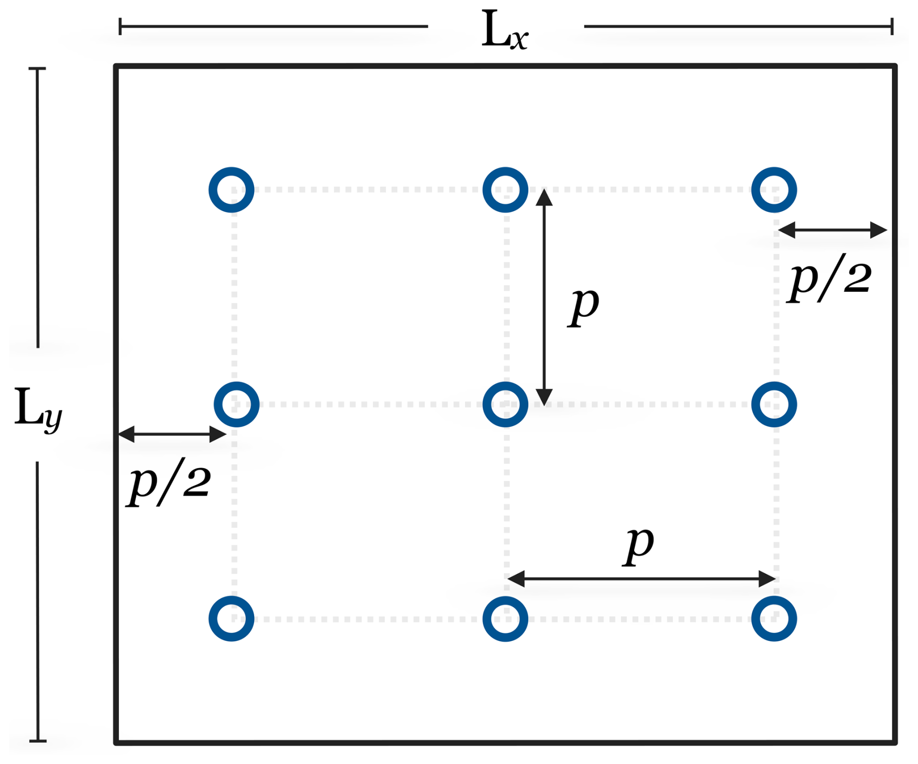
The mesh consists of a square box with longitudinal, crosswise, and vertical dimensions of $L_x\times L_y\times L_z=\mathrm{3}H\times \mathrm{3}H\times H$ with H=1280 m. In the horizontal plane, cells are uniformly distributed with $N_x\times N_y=\mathrm{548}\times \mathrm{548}$ cells, yielding a resolution of ${\mathrm{\Delta }}_x={\mathrm{\Delta }}_y\approx \mathrm{7}$ m. In the vertical direction, the mesh is constructed like this: a uniform mesh resolution of Δ_z=5 m up to z=130 m – above this height cells are stretched at a rate of ≈1.037. The mesh is then vertically refined by halving the cell height in two subsequent steps: first within the region of cells below z=80 m and then once more for all cells below z=40 m. This yields a vertical cell resolution of Δ_z=1.25 m below 40 m – within and above the forest – Δ_z=2.5 m between 40 m $\le z\le \mathrm{80}$ m, and Δ_z=5 m between 80 m $\le z\le \mathrm{130}$ m and a total of N_z=116 cells for a total of $N\approx \mathrm{35.8}\times {\mathrm{10}}^{\mathrm{6}}$ cells. A slight modification to the vertical zone covered by the second refinement was needed for the cases with larger roughness lengths (z₀=0.5 and 0.65 m) to avoid it coming too close to the height of the first node, i.e. to prevent $z_{\mathrm{1}}={\mathrm{\Delta }}_{z,\mathrm{1}}/\mathrm{2}\approx z_{\mathrm{0}}$. In those cases – described in Sect. 6.1 – the second refinement starts at z=2.5 m instead of z=0. All the lateral boundaries are set to periodic, whereas the top boundary is a symmetry plane. The flow is driven by a pressure gradient with a fixed geostrophic wind of u_g=9 m s⁻¹ in the longitudinal direction (equivalent to φ=270°). Simulations are first run over a domain with a mesh without the two vertical refinement processes (so Δ_z=5 m is maintained up to z=130 m), and z₀=0.03 m during 320×10³ s. The resulting fields are then interpolated onto the vertically refined mesh, where the simulation is run for an additional 120×10³ s, employing the modelling features of the given verification case. These runs employ a varying time step Δt, calculated as to maintain a domain maximum Courant–Friedrichs–Lewy number of CFL ≲0.85. Considering that the simulations yield a mean velocity magnitude ${\stackrel{\mathrm{‾}}{u}}_s$ of approximately 5 m s⁻¹ at 100 m, this period is equivalent to about 156 longitudinal flow-through times (LFTT) or almost 469 eddy-turnover times $H/{\stackrel{\mathrm{‾}}{u}}_s$. Convergence of fourth-order moments of velocity at heights up to 500 m is observed during this period. Lastly, simulations are run with a fixed Δt=0.14 s during 20×10³ s to gather velocity time series and average fields for sampling (26 LFTTs, 78 eddy-turnover times). The latter is carried out along vertical lines arranged in a layout as shown in Fig. 1. u_i is sampled at every cell centre along each of the nine columns.

Figure 1 Layout of the sampling positions over the horizontal plane of the domain for setup 1 (Sect. 4.2.1). The circles represent the positions of the nine vertical lines where the velocity is sampled at every cell centre. The lines are evenly separated by a distance p=H.

4.2.2 Numerical setup 2: Ryningsnäs simulations

Three different domains are used, with the longitudinal direction L_x aligned with each incoming wind direction φ. For every case the domains are square boxes of $L_x\times L_y\times L_z=$ 32 km ×20 km $\times \sim \mathrm{1.2}$ km. The met mast is located at d_MM=20 km in the longitudinal direction, in the middle of the spanwise plane. The mesh is constructed with three regions of different resolutions in the horizontal plane, referred to as farm where the resolution is the highest, buffer with coarse cells at the outer edge of the domain, and transition where cells stretch in between the former regions. A top view of the computational domain is presented in Fig. 2 (left), showing the innermost farm region $L_x^{\prime }\times L_y^{\prime }=\mathrm{20}$ km ×12 km, the transition (between the farm and the dashed rectangle), the buffer region (the edge outward from the dashed rectangle), and the overall horizontal dimensions of the domain L_x×L_y. The widths of the transition and buffer edge regions in the longitudinal and spanwise directions are $W_{t,x}=\mathrm{3}$ km, $W_{t,y}=\mathrm{2.5}$ km, ${\mathrm{W}}_{b,x}=\mathrm{3}$ km, and $W_{b,y}=\mathrm{1.5}$ km, respectively. Figure 2 (middle) shows the horizontal plane of the 240° case, with the colour scale corresponding to the terrain elevation, also indicating the distance to the met mast, d_MM, as the sum of the widths of the buffer, transition, and the $d_{\mathrm{MM}}^{\prime }=\mathrm{14}$ km (location of the met mast from the edge of the farm region). As shown in the figure, the elevation becomes flat within the inmost 500 m buffer, so the elevation is equal at the outermost boundary, corresponding to 63.06 m above sea level (100° case), 163.25 m above sea level (240°), and 137.76 m above sea level (290°). The horizontal-cell resolution in the farm region is ${\mathrm{\Delta }}_x={\mathrm{\Delta }}_y=\mathrm{25}$ m (squared cells), stretching toward the buffer region where cells are also squared with 250 m per side. The height of the first cell ${\mathrm{\Delta }}_{z_{\mathrm{1}}}$ at the met mast location is about 3.4 m in all cases, with cells stretching in the vertical direction at a uniform rate of approximately 1.05. The variations in elevation in the terrain covered at each wind direction cause the domain height L_z and vertical number of cells N_z to be slightly different: 1.172 km and 84 cells for the 100° case, 1.305 km and 86 cells for 240°, and 1.267 km with 85 cells for 290°. Thus, mesh sizes, in millions of cells, are ≈40.85 (100°), ≈41.81 (240°), and ≈41.33 (290°). The mesh is created using CENER-WindMesh (Gancarski and Chávez-Arroyo, 2017; Ivanell et al., 2018). The adequacy of the grid resolution is discussed in the Results section.

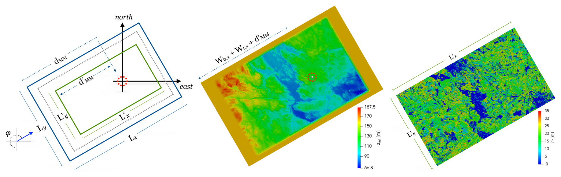
Figure 2 Computational domain in the horizontal plane employed for the Ryningsnäs simulations, as described in Sect. 4.2.2 and 4.2.3. The dashed circle denotes the location of the met mast. Left: dimensions of the domain and the farm region (prime labels). Middle: terrain elevation, with labels indicating the extensions of the different mesh sections with respect to the met mast location. Right: tree height within the farm region. All images correspond to the 240° wind direction case.

The ASL-derived forest density map is used to create the PAD field within the farm and transition zones by linearly interpolating between the 10 m × 10 m input fields and the mesh. In the buffer, a uniform value of PAD=2.813 1 m⁻¹ is set within a constant tree height of 14.38 m, corresponding to the average height of the forest in the input map. The ground surface is set as a wall with a uniform roughness of z₀=0.03. All the lateral boundaries are set to periodic, so the flow is recycled as it leaves the outlet and the sides. Simulations are run under neutral conditions, with the top boundary set as a symmetry plane. The flow itself is driven by a constant and vertically uniform pressure gradient that is calculated on the basis of the geostrophic velocity vector u_g (see Bautista, 2015), in addition to a Coriolis forcing corresponding to a latitude of 57°. To find the right magnitude and direction of u_g for each case, a calibration procedure was devised, with the goal of approximating the desired target velocity of $\left|\stackrel{\mathrm{‾}}{\mathit{u}}\right|=\mathrm{7.4}$ m s⁻¹ and the given wind direction φ at z_agl=100 m (height above ground level) at the met mast location. It starts by finding u_g that yields the desired target velocity in a preceding run over a domain with the same dimensions and numerical parameters but with a coarser mesh of 50×50 m horizontal resolution within the farm region. That u_g vector is then used to drive the simulations (above the described mesh), with an initial velocity field of zero. Subsequent adjustments to u_g were made up until 240×10³ s, and from then on, simulations were run with a fixed u_g for a total of 400×10³ s. The convergence of the flow solution was verified to have been fulfilled by observing that profiles of ${{\stackrel{\mathrm{‾}}{u}}_i^{\prime }}^{\mathrm{2}}$, calculated in successive periods of 20×10³ s, had reached a quiescent state. Velocity time series and other data employed for the results are extracted during a subsequent sampling period of 20×10³ s to the initial run at every cell centre on a vertical column at the met mast location. For this, a fixed time step of Δt=0.296 s was used, corresponding to a maximum Courant–Friedrichs–Lewy number over the whole domain of CFL≈0.6. The geostrophic wind vector derived from the calibration procedure and the averaged velocities obtained during the sampling period are shown in Table 1.

Table 1 Mean velocities and directions at z_agl=100 m and the geostrophic wind employed in driving the flow for the Ryningsnäs cases.

4.2.3 Numerical setup 3: assessment of terrain and forest conditions on footprint

An additional set of simulations is carried out with the objective of evaluating the effects that the representation of the terrain and forest features have on the prediction of the wind characteristics at a given location. Based on the domain layout employed in Sect. 4.2.2 for the incoming direction of 240° (identified as R3.0), three additional setups, labelled R3.1 to R3.2, with the exact same dimensions are created but with the following distinctive configurations:

1. R3.1 is a domain where the ALS-obtained PAD distribution, i.e. the realistic forest, is constrained to a smaller area around the met mast, extending 3 km + 2 km (upstream + downstream) in length and 5 km in width. Outside this region, the forest density is uniformly set to the approximate average value of the forest density upstream the met mast for the 240° direction, PAD=0.12 m⁻¹, with a height equal to 14.38 m (the mean of the forest map).

2. R3.2 is a domain with a flattened ground, with a constant elevation set to 122.67 m above sea level, equal to the terrain elevation at the location of the met mast. The forest distribution is the same as in the reference 240° configuration, R3.0.

3. R3.3 is a domain with a uniform forest distribution, PAD=0.12 1 m⁻¹, with a constant height of 14.38 m. The terrain elevation is the same as in the reference 240° configuration, R3.0.

In cases R3.1 and R3.3, the mesh is the same as in the 240° reference case, while for case R3.2, a slight variation in the vertical direction occurs due to the flattening of the elevation differences at the ground. The latter has N_z=85 cells with the first node at z₁=1.778 m, in comparison to the values of the reference 240° case of N_z=88 cells and z₁=1.727 m. Cases R3.1 and R3.3 have one caveat: a fully uniform tree height would require a uniform layer of cells at the canopy top that is not possible to obtain for such a short height above a terrain with the complexity of the chosen site. However, as the mesh is the same as the one used in the reference 240° case set with a realistic PAD distribution, the comparison with that case is made over terrains representing the same complexity and its ensuing effects on the wind above. In cases R3.1 to R3.3, the flow is driven by the same parameters as in the 240° case (Table 1) with the same boundary conditions. Simulations are run during 240×10³ s to attain flow convergence and then, as in the 240° reference case, during an additional 20×10³ s period with Δt=0.296 s to record velocity time series and other data at every cell centre along a vertical column at the met mast location.

5 Post-processing

This section describes the post-processing, and unless explicitly stated, this was performed in the same way for the measurements and the simulations. For the measurements, the time series was split into 30 min long periods with a sampling rate of 20 Hz. In order to retrieve comparable data from the simulations, the time series sampled from the vertical array described in Sect. 4.2.1 were used. At each height the reference frame was rotated according to the direction of the local mean wind in the same way as described in Sect. 3.2. Fluctuating variables were also constructed in the same way, with the difference that the whole 20 000 s period was regarded as the averaging period. Tests were also carried out by splitting the LESs into 30 min blocks, which did not visibly impact the results, apart from the obvious effect of filtering out low frequencies in the spectra.

Statistical processing for the measured turbulence was the same as in Arnqvist et al. (2015), with the most important steps repeated below for convenience. The 20 Hz data were split into 30 min bins, after which fluctuations were constructed by removing the arithmetic mean. The data were rotated locally (i.e. at each height and 30 min period) into the direction of the horizontal mean wind, with u, v, and w describing the streamwise, spanwise, and vertical wind, respectively. Higher-order moments were constructed by multiplication of fluctuation velocities, for example the streamwise shear stress: $\stackrel{\mathrm{‾}}{u^{\prime }{w}^{\prime }}$, where $u^{\prime }=u-\stackrel{\mathrm{‾}}{u}$ and $w^{\prime }=w-\stackrel{\mathrm{‾}}{w}$ are the fluctuating streamwise and vertical velocities, and the overbar denotes temporal average.

5.1 Spectral statistics

Spectral statistics were calculated by a fast Fourier transform (FFT). A cross-spectral tensor, $\mathit{\varphi }(u_i,z_k,u_j,z_l)$, was created for all possible separations along the met mast ($z_k\in [\mathrm{40},\mathrm{59},\mathrm{80},\mathrm{98},\mathrm{120},\mathrm{138}]$ m height) and variable combinations $(u_i\in [u,v,w\left]\right)$ by taking the outer product of all velocity component transform signals (FFT of u^′, w^′, or v^′ at all measurement heights) with their complex conjugates. The spectral tensor and frequency vector were then averaged in 20 logarithmically spaced frequency bins for each 30 min time series. To examine how realistic the LES turbulence would appear for a hypothetical wind turbine rotor, some specific cross-spectral measures were used.

Single-point power spectra and cospectra, $\mathrm{\Re }\mathit{\varphi }(u_i,z_k,u_j,z_k)$, were used to evaluate the impact of the filter scale on the characteristics of single-point turbulence. The spectral density was premultiplied by the frequency and normalized by the total turbulence kinetic energy. The frequency was normalized by multiplication by $z_k/U_k$.

To evaluate the effect of turbulence on larger sections of the rotor, the two-point cross-spectra, $\mathrm{\Re }\mathit{\varphi }(u_i,z_k,u_i,z_l)$, and the coherence,

$$\begin{array}{}\text{(17)}& \mathrm{Coh}(u_i,z_k,u_i,z_l)={\displaystyle \frac{\left|\mathit{\varphi }\right(u_i,z_j,u_i,z_k){|}^{\mathrm{2}}}{\mathit{\varphi }(u_i,z_k,u_i,z_k)\mathit{\varphi }(u_i,z_l,u_i,z_l)}},\end{array}$$

were examined.

To determine the slope of the eddies, the phase lag in radiance was examined between two different heights, z_j and z_k:

$$\begin{array}{}\text{(18)}& \mathrm{\Delta }\mathit{\theta }(u_i,z_j,u_i,z_k)=\arctan \left({\displaystyle \frac{\mathrm{\Im }\mathit{\varphi }(u_i,z_k,u_i,z_l)}{\mathrm{\Re }\mathit{\varphi }(u_i,z_j,u_i,z_k)}}\right).\end{array}$$

For the statistics processing of LES from Sect. 4.2.1, sampling probes are located at each cell centre over the nine-column layout as in Fig. 1. Spectra, integral timescales, and high-order statistical quantities are presented as horizontal-plane averages, i.e. the average of all nine values at the same height. In the case of coherences, the average is made over nine location pairs. The supplementary logarithmic average applied to spectra is referred to as smoothing as well.

5.2 Integral timescales

Integral timescales were calculated for both the simulations and the measurements by taking the FFT of the spectral density and dividing it with the variance to find the auto-correlation function (Wyngaard, 2010, Eq. 15.14). The value of the integral timescale, 𝒯, was then estimated by finding the time lag for which the auto-correlation fell below exp (−1), in accordance with Kaimal and Finnigan (1994). Other methods of finding 𝒯 were also tested and gave similar results. The lengthscales are obtained simply by multiplying by the mean velocity at each location.

5.3 Confidence levels

5.3.1 Measurements

Confidence levels around the long-term mean values were estimated by the standard error of the 30 min averages. Levels of 95 % were estimated as 1.96 of the standard error, assuming that each 30 min mean is statistically independent of the others and that the 30 min means are normally distributed around the long-term mean.

5.3.2 LES

When comparing with measurements, confidence levels are also calculated for LES (Sect. 6.2 and 6.3). Since the mean values for the LES data were constructed from a single time series, the confidence levels were determined differently from the measurements. For the mean wind, the relative random error variance, e_u, of the time series was estimated following Lumley and Panofsky (1964) by

$$\begin{array}{}\text{(19)}& e_u={\displaystyle \frac{\mathrm{2}{\mathcal{T}}_{\mathrm{1}}\stackrel{\mathrm{‾}}{{u^{\prime }}^{\mathrm{2}}}}{T{\stackrel{\mathrm{‾}}{u}}^{\mathrm{2}}}},\end{array}$$

where T is the length of the time series, and 𝒯₁ is the integral timescale of u. For the second- and third-order moments, the formulation from Lenschow et al. (1994) was used:

$$\begin{array}{}\text{(20)}& e_{\stackrel{\mathrm{‾}}{u_i{u}_j}}={\displaystyle \frac{\mathrm{2}{\mathcal{T}}_{ij}}{T}},\end{array}$$

where 𝒯_ij, the integral timescale for the covariance, was estimated as ${\mathcal{T}}_{ij}\approx \sqrt{{\mathcal{T}}_i{\mathcal{T}}_j}$. Only the isotropic third-order moments were evaluated, and here we also follow Lenschow et al. (1994):

$$\begin{array}{}\text{(21)}& e_{\stackrel{\mathrm{‾}}{u_i^{\mathrm{3}}}}\approx {\displaystyle \frac{\mathrm{6}{\mathcal{T}}_i}{T}}.\end{array}$$

The first- and second-order velocity moments have been normalized by the kinetic energy at the scaling height, so to derive appropriate confidence intervals, the relative random errors were first raised to the exponent $\mathrm{1}/\mathrm{2}$, then multiplied by the dimensional quantity of interest and normalized again by the scaling factor. Finally, it was assumed that the uncertainty follows a Gaussian distribution so that 95 % confidence levels could be obtained by multiplication by 1.96. To give an example, the confidence interval of the horizontal variance was calculated by $(\mathrm{2}{\mathcal{T}}_{\mathrm{11}}/T{)}^{\mathrm{1}/\mathrm{2}}\stackrel{\mathrm{‾}}{u^{\prime }{u}^{\prime }}/k_{\mathrm{sc}}$. It should be noted that this procedure omits the random error due to the statistical uncertainty in the scaling factor, which was neglected due to difficulties in estimating its correlation with the random error of the investigated variable itself. Since most scaled variables are 𝒪(1), this added uncertainty could be expected to contribute to a widening of the confidence intervals by a factor between $\sqrt{\mathrm{2}}$ and 2 depending on the correlation between the random errors (assuming standard error propagation rules for division and equal sizes of the relative random error). Given the already approximate nature of the confidence interval estimation, this was not added, and the confidence intervals should only be considered an indication of the statistical uncertainty.

6 Results

6.1 Wall model and forest implementation and study

The first part of the Results section comprises the simulation of the wind flow over ideal conditions of terrain and forest coverage to observe the performance of the numerical model and see its validity. Specifically, variations in the SGS model, PAD, and z₀ are deliberately chosen to yield contrasting turbulence features in each case. The cases are listed in Table 2. These can be grouped into three categories according to the verification purpose:

1. to compare the results produced by the forest model with those produced by a wall model that only employs z₀

2. to assess whether there is an impact on the wind flow produced by varying the ground roughness in a simulation that also employs PAD-based drag

3. to examine the effect of varying the tree density within the forest (this comprises the observation of the significance of including an enhanced subgrid dissipation term for the forest – ε_SGS,f in Eq. 13).

Table 2 Simulation cases for model verification. Cases F1 to F8 employ an explicit model of the forest, while F8 and F9 only use a wall model without a forest representation.

The simulations are run based on the numerical setup described in Sect. 4.2.1, employing a flat-ground surface with – for the applicable cases – a uniform roughness and/or a forest of uniform tree height of h_f=20 m. In most cases with forest, PAI=3 is used, yielding a tree density of PAD=0.15 1 m⁻¹. This is the value employed in reference case F1. In two other cases (F6, F7), PAI=0.36, corresponding to PAD=0.018 1 m⁻¹, which is used as the value for the low-density cases. The roughness length and displacement height in case F9 are calculated from parameterizations that provide a tuning-free, diagnostic estimation based only on forest density and height (Mohr et al., 2018, Eqs. 9–16 and 9–17). For a forest with PAI =3 and a height of 20 m, this yields z₀=0.65 and a displacement height of d=17.01 m. The relatively short roughness length is a result of the lack of roughness sublayer correction, which would require empirical calibration. Results from this case, also referred to as PAI derived, are shown with an upward shift, i.e. z+d.

6.1.1 Impact of modelling parameters on flow characteristics

Figure 3 compares the results of the profiles of the velocity magnitude and wind direction between the forested cases (F1, F7) and setups without an explicit forest representation (i.e. without a PAD field) but with a rough surface at the bottom, simulated by means of a wall model. For the latter, two roughness values have been chosen, the z₀=0.03 m used for the reference model (case F8) and a value that has been derived as the PAI-derived z₀=0.65 m (F9). Case F7 is also included to observe the influence of high roughness in a forest with low density. The results in Fig. 3a–b for the horizontal mean velocity magnitude u_s (used henceforward without a bar) show that the drag effect is the largest everywhere for reference case F1 and the smallest for F8, as expected. The PAI-derived roughness in F9 produces results that are noticeably different from the reference case. Even when considering the displacement height, a match is seen until about 850 m. The use of low PAD and high z₀ in F7 results in a velocity profile with a slope opposite to F1 and values of u_s in between those of F1 and F9, showing evidence of the effect of the high roughness within the low-density forest. The same z₀ is not seen to produce the same result with a higher PAD (case F2), as seen below. Figure 3c displays a comparison of the turning of the wind within the forest, where φ=270° corresponds to a flow moving in the longitudinal direction, aligned with the x axis of the domain. The turning is seen to be the largest for F1, with the low-PAD and wall-model-only cases showing much less deviation in comparison. Notably, the low-PAD case F7 displays minimal turning but a distinct wind direction that denotes the influence of the drag of the forest, despite its low density, on setting the wind direction above it. Also, it is worth noting that the wind direction above the forest cannot be reproduced by the PAI-derived roughness simulation. Figure 3d compares the total TKE, highlighting the differences produced within the forest due to the PAD variation or its absence. In spite of this, F7 quickly reaches the same level as F1 above the canopy due to the higher flow velocity. Meanwhile, the non-forested cases F8 and F9 show a significantly lower level in comparison.

Figure 3 Comparison of the horizontal velocity magnitude over the entire domain height (a) and the first 150 m (b), wind direction (c), and total TKE (d) between cases with explicit forest modelling (F1, F7) and those with only a wall model (F8, F9). The vertical region covered by the forest is displayed as a green-shaded area.

Figure 4 compares the velocities, vertical wind shear $\mathrm{d}{u}_s/\mathrm{d}z$, resolved TKE k_res, and its ratio with respect to the total amount $k_{\mathrm{tot}}=k_{\mathrm{res}}+k_{\mathrm{SGS}}$ between the reference forest model (F1) and forest models with higher roughness (F2) and lower PAD (F6 and F7). The reduced forest drag of the latter leads to an acceleration of the wind profiles, as expected. Inside the canopy, the velocity profiles of the low-PAD cases F6 and F7 can be regarded as an intermediate point between the u_s curves of a wall-model-only case (F8 in Fig. 3b) and the reference PAD case F1, where the region near the top of the forest layer drives a change in the concavity of u_s. This can be recognized as a feature of the transition between a boundary layer and the mixing layer that arises when forest density increases (Raupach et al., 1996). A key aspect of the mixing layer analogy for forest flows is the inflection point in the velocity profile near the canopy top, clearly seen in F1 and in other cases with the same PAD. In Fig. 4 it can also be seen that despite the increased z₀ in F2 compared to that of F1, the PAD value seems large enough as to control the flow characteristics and produce nearly identical results within the forest and above, except for the first couple of cells above the ground, where k_SGS for F2 is slightly larger, shown indirectly via $k_{\mathrm{res}}/k_{\mathrm{tot}}$. Conversely, PAD in cases F6 and F7 is lower, and the different values of z₀ produce discernible variations within the forest, especially in vertical shear, but only in the case of u_s is the difference also maintained above the forest. Furthermore, while the near-ground fluctuations are mostly resolved by the LES in cases F1 and F2, the lower PAD in F6 and F7 causes a noticeable increment on the SGS component, observed as a strong reduction in $k_{\mathrm{res}}/k_{\mathrm{tot}}$, as shown in Fig. 4d. Note that in this figure, it is possible to see the transition between the mesh refinement zones at z=40 and 80 m (see Sect. 4.2.1), but this has no effect on the results and their analysis.

Figure 4 Variation in modelling parameters in cases with explicit forest modelling. From left to right: velocity (a), vertical wind shear (b), resolved TKE (c), and resolved to total TKE ratio (d).

The next comparison focuses on the impact of the modelling choice for the subgrid component within and above the forest. Figure 5 shows vertical profiles of u_s, k_res, and k_SGS and the ratio of resolved to subgrid $k_{\mathrm{res}}/k_{\mathrm{tot}}$ for cases F1 to F5, all of which use the same PAD value. In spite of all variations in near-wall treatment, the velocity profiles yielded by all these setups are essentially identical. Also, it can be seen that k_res is nearly equal above the forest, except for a minor increase from the Smagorinsky SGS model in F5. More differences can be appreciated in k_SGS. For that, the absence of the extra dissipation term (Eq. 15) in F4 shows an ensuing increase in the subgrid turbulence component, which can also be observed as a reduction – with a minimum just below the forest edge – in the profile of $k_{\mathrm{res}}/k_{\mathrm{tot}}$. This occurs only within the forest, the only region affected by the dissipative term ε_SGS,f of Eq. (15). The use of Smagorinsky, which also lacks ε_SGS,f, is shown to produce a greater increase in k_SGS but only around the forest edge. Note that Smagorinsky is employed without a wall model, which permits us to analyze its performance within the forest separately from that near the ground.

Figure 5 Variation in turbulence modelling values. From left to right: velocity (a), resolved TKE (b), subgrid TKE (c), and resolved-to-total ratio of TKE (d) for the forested cases.

The results of F5 show a reduction in the resolved portion of the turbulence, peaking at the forest edge as well. It can also be seen that using Smagorinsky leads to a slight increase in k_res above the forest that persists along the ABL height (here shown only for the first 150 m). This result is consistent with the observations of overdissipation yielded by this model near the ground, but since no rough surface is used, such effect is then emphasized from the forest edge and above. It has been argued that overdissipation can lead to an overestimation of the mean velocity in the lower parts of the ABL (Porté-Agel et al., 2000; Pope, 2000). However, neither Smagorinsky nor other modelling variations (F1 to F5) are observed here to affect the velocity profile noticeably, neither within nor above the forest. Furthermore, except for the Smagorinsky model, the level of total turbulence kinetic energy does not appreciably change between the different modelling choices. Although none of the subgrid models discussed here account for the anisotropy in the flow (as discussed in Sect. 4.1), their effect is anticipated to be minor since anisotropies in wind turbulence are significantly reduced toward the interior of the canopy in comparison to the region above (Arnqvist, 2013).

6.1.2 Spectral analysis

The next part of the study focuses on the turbulence characteristics of three simulation cases: the reference case F1 as well as F6 and F9. This permits us to contrast the results of simulations that explicitly consider forest – with two different densities – with one that instead employs a PAI-derived ground roughness. The one-point spectral properties are examined first; these are calculated from the full time series of the LES (see Sect. 4.2.1) at different heights following the methods described in Sect. 5.1. To facilitate the visualization, each curve is smoothed by applying a further averaging using 25 bins logarithmically distributed. It is possible to observe the effect of the smoothing procedure as the non-smoothed spectra of the reference case are also shown in each figure. Spectra are shown at heights of 25, 100, and 200 m, to represent the near forest and typical turbine positions. Displacement height is considered for case F9, subtracting the value of d from these positions.

The auto-spectra of the longitudinal fluctuations are shown in Fig. 6 together with reference slopes of $-\mathrm{5}/\mathrm{3}$ for the inertial subrange and −1 for the intermediate range between inner and outer scales (Katul et al., 2012). While the power spectra at 25 m display what appears to be two separate scaling regions, at 100 and 200 m heights, a substantial frequency range exhibits a slope in between −1 and $-\mathrm{5}/\mathrm{3}$. Whereas the power spectrum of the low PAD remains very similar to that of the reference case for all heights, case F9 displays a noticeably lower level of energy for most of the scales except for the lowest height, an outcome consistent with the comparison of k_tot in Fig. 3. While this supports the ability of the wall model – with consideration of the displacement height – to represent the energy distribution of longitudinal velocities for lower regions, it underestimates it for regions covered by a wind turbine rotor.

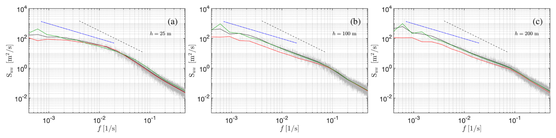
Figure 6 Power spectral density of the longitudinal velocity at z≈25 m (a), 100 m (b), and 200 m (c). The pre-smoothed spectra of F1 are shown as a grey line. The dashed line corresponds to the $-\mathrm{5}/\mathrm{3}$ slope and the dashed–dotted line to −1.

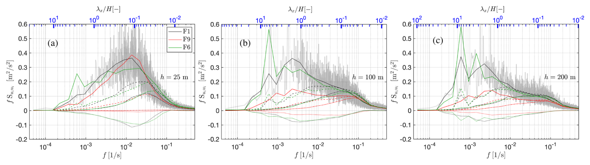
Figure 7 Comparison of premultiplied power spectral density of uu (solid lines), vv (dashed), and ww (dot-dashed) fluctuations and cross-spectral density uw (dotted) fluctuations for the heights of 25 m (a), 100 m (b), and 200 m (c). The pre-smoothed uu spectra of F1 are shown as a grey line. The top axis shows a streamwise lengthscale, calculated using u_s of case F1.

Figure 7 shows the frequency-premultiplied cospectra of uu, vv, and ww and the cross-components uw at different heights. This permits us to observe the proportions in energy content between the different components for each setup, as well as their energy distribution as a function of frequency. As expected, longitudinal fluctuations observe the largest levels of energy, followed by the lateral, vertical, and cross-component uw. A redistribution of energy toward smaller frequencies is observed when the height increases, with the spectra maxima moving toward the left. This can be seen in all components except for ww, in part due to the difficulty of resolving the small vertical fluctuation scales (considerably smaller than those in the horizontal components) at this level of mesh refinement. Instead, the energy of the ww spectra becomes somewhat more distributed (or flattened) along the frequencies. The spectral energy of ww and uw of case F9 is close to zero for the lowest elevation due to its proximity to the ground that limits the size of the eddies. Yet, their values at 100 m and 200 m remain distinctly lower compared to F1 and F6. Something similar occurs with the energy of the lateral fluctuations vv, which is persistently smaller for F9 than for the other cases. Furthermore, a strong decay in energy in longitudinal velocities can be seen for case F9 from the 25 m height in Fig. 6a in comparison with (b) 100 m and (c) 200 m. These differences reveal contrasting characteristics in the representation of turbulence when representing forest drag compared to an approach based exclusively on a wall model. Notably, the lower energy levels in uw reflect limited strength of the momentum flux. Conversely, the spectral curves of F1 and F6 show similar values in all components despite the differences in leaf density. Two key distinctions can be discerned. Firstly, it is found in ww at the 25 m height, where the maximum energy of F6 is somewhat greater and also positioned at higher frequencies. This arises from the larger permeability to vertical velocities due to the lower PAD. The second distinction concerns the intensity and position of peaks. Indeed, horizontal components show prominent peaks at frequencies $\sim \mathrm{6}\times {\mathrm{10}}^{-\mathrm{4}}$ and $\sim \mathrm{2}\times {\mathrm{10}}^{-\mathrm{3}}$ s⁻¹, which can be associated with the dimensions of the domain. The first one corresponds to a time event of about 1667 s, linked to the recycling period of the flow in the domain, covering a distance slightly larger than L_x according to the wind directions shown in Fig. 3. This peak is more prominent for F6, pointing to a stronger effect of the recirculation for lower forest densities. The second peak occurs for events of approximately 500 s, which would correspond to the eddy turnover time $\sim H/U$. Therefore, this peak signals the scale of the largest structures in the simulation, indicating the location from where the energy decays toward smaller values at larger frequencies. To support the analysis, a secondary x axis is included at the top of Fig. 7, showing a streamwise wavelength normalized with the ABL height ${\mathit{\lambda }}_x/H=u_s/\left(fH\right)$, with u_s corresponding to the mean velocity of case F1 at the given height. This facilitates relating the relevant events to their characteristic lengthscales. While the previous observations are consistent with these scales, it can also be readily seen which are the largest lengthscales that peak in the domain (${\mathit{\lambda }}_x/H\approx \mathrm{5}\sim \mathrm{8}$ in Fig. 7b and 7c, respectively, increasing from ${\mathit{\lambda }}_x/H\approx \mathrm{1}$ at z=25 m in Fig. 7a) or the smallest (${\mathit{\lambda }}_x/H\approx \mathrm{5}\times {\mathrm{10}}^{-\mathrm{2}}$ for ww in Fig. 7a, whose peak broadens for increasing heights).

When assessing the footprint of forest or terrain, it is necessary to account for the presence of other coherent structures moving through the ABL that persists over large spans of the domain. Hutchins and Marusic (2007) provided experimental evidence of “very long, meandering structures of positive and negative streamwise velocity fluctuations”, streak-like features in the surface layer of turbulent boundary layers in wind tunnels and in the atmospheric surface layer (ASL) over a flat, low-roughness terrain, which extend up to about 20δ, where the ASL height is δ≈60 m. The follow-up studies by Hutchins et al. (2012) also report experimental evidence of “highly elongated low/high speed regions” identified as very large scale motions (VLSMs) that extend beyond 10δ in the streamwise direction, in both the laboratory and measurements, on the atmospheric surface layer. By means of a similar spectral analysis of LES of neutral, flat ABL, Fang and Porté-Agel (2015) show that uu power spectra display a bimodal distribution, with one wavelength peak at ${\mathit{\lambda }}_x/H\approx \mathrm{3}$ corresponding to large-scale motions, whereas an additional, longer wavelength peak ${\mathit{\lambda }}_x/H\approx \mathrm{20}$ is associated with VLSMs. For the spanwise and vertical directions, there is one peak at about ${\mathit{\lambda }}_x/H\approx \mathrm{0.8}$ and 0.4, respectively.

The calculation of coherence permits us to quantify the maximum correlation of the velocity component at a given turbulence scale. Spectral coherences are calculated for cases F1, F6, and F9 for three different vertical separations δ_z=20, 40, and 80 m, set within the hypothetical rotor area. This is done using Eq. (17), based on the calculation of the two-point cospectrum and one-point spectrum of the two locations. As pointed out by Kristensen and Jensen (1979), it is required that the calculation of spectra includes a procedure resembling an ensemble average, in this case block average, to avoid that the resulting coherence takes a value of unity for all frequencies. Therefore, the time series at each sampling point is divided into blocks of about 1 h duration with 50 % overlap, from which individual spectra are obtained and later averaged. The process is repeated for each of the nine locations of equal height, whose average yields a single spectrum. Finally, this spectrum is logarithmically smoothed with the procedure described earlier. All spectra used in Eq. (17) are obtained in this way, yielding the coherences shown in Figs. 8 to 10. To observe the effect of smoothing in the calculations, the figures also include the coherence obtained with spectra that have not been smoothed but only for case F1. The coherences of longitudinal velocities obtained with the model of Davenport (1961) included in the standard by IEC (2019) are shown for comparison.

Figure 8 Coherences of longitudinal (a), lateral (b), and vertical (c) fluctuations for a vertical separation of δ_z≈20 m. The coherence from the pre-smoothed spectra of F1 is shown as a grey line. The dashed line in (a) corresponds to the coherence model of the IEC (2019).

Figure 9 Coherences of longitudinal (a), lateral (b), and vertical (c) fluctuations for a vertical separation of δ_z≈40 m. The coherence from the pre-smoothed spectra of F1 is shown as a grey line. The dashed line in (a) corresponds to the coherence model of the IEC (2019).

Figure 10 Coherences of longitudinal (a), lateral (b), and vertical (c) fluctuations for a vertical separation of δ_z≈80 m. The coherence from the pre-smoothed spectra of F1 is shown as a grey line. The dashed line in (a) corresponds to the coherence model of the IEC (2019).

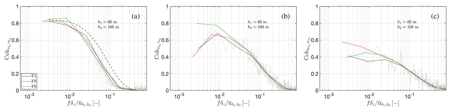
For the first separation of 20 m, between h₁=80 and h₂=100 m, the energy distribution represented by the coherence of the longitudinal velocity component is shown in Fig. 8a. There, differences are rather minimal between the outcomes of the three different setups while comparing well to the IEC prediction, except for the highest decade of normalized frequencies. Figure 8b and c compares results for the lateral and vertical velocity components, respectively, showing a large correspondence between coherences of F1 and F6, while those of F9 are slightly lower. For the 40 m separation, longitudinal coherences in Fig. 9a are again very close among the different setups. These curves show a small drop in correlation compared to the 20 m separation but also a lower value than the projection of IEC that now extends over a large part the frequency range. In Fig. 9b the distinct maxima of coherence of setups F1 and F9 reveal that turbulence structures have a characteristic lateral extension that is shorter compared to that of F6. Figure 9c shows a noticeable drop in the maximum coherence of the vertical motions, seemingly due to a structural tilt in turbulence and phase changes with height, which become more evident with increasing separation. The drop occurs for the three cases, although case F9 stands out due to its greater value around the smallest frequencies. The same trends are observed for the largest separation of 80 m. Figure 10a shows a small reduction in longitudinal correlation, with the values remaining consistent among all cases and largely below the value predicted by the IEC curve. Figure 10b displays the correlation maxima related to the limited lateral extension of the turbulence structures, with F6 being the largest (as in the previous case δ_z=40 m) but with F9 now exhibiting a more pronounced drop than case F1. Figure 10c shows that correlations of vertical velocities continue to decrease, with F9 showing the highest values.

In general, results shown in Figs. 8, 9, and 10 display a strong coherence for the longitudinal velocity component along the frequency range for all cases, which is largely maintained for the three separations. Conversely, lateral and vertical components show a strong correlation only for the smallest separation of δ_z=20 m. For δ_z=40 and 80 m, the shape of coherences of the lateral component suggests that the turbulence structures have a characteristic width, which is the largest for F6 and the smallest for F9. For the vertical velocity component, the coherence decreases more markedly with increasing separation, but less so for case F9. On one hand, this reflects the need for a larger mesh refinement to reproduce the comparatively smaller velocity fluctuations in this direction. But more significantly, the larger values displayed by F9 give an indication that the greater shear in the forested cases produces a stronger distortion in the eddies, reducing their coherence in that direction. This supports what was already determined from the spectral results in Fig. 7: cases with an explicit forest modelling can change not only the energy level of vertical fluctuations but also its distribution, a feature that is not replicated by a roughness-based modelling approach. For the lateral correlations, a more significant drop is noted, pointing to an underestimation of the width of the eddies by the wall model F9, which accompanies the greater one-point spectral density of the lateral velocities observed in Fig. 7 from the forest models in comparison to F9.

Lastly, the smaller coherence values consistently displayed in the longitudinal direction with respect to the IEC standard represents an interesting outcome. Coherences obtained from experimental results also show correlations below the IEC prediction, for different separations (Sect. 6.2). In all these cases, results are displayed with a normalization for the frequency axis, where ${\stackrel{\mathrm{‾}}{u}}_{h_{\mathrm{1}},h_{\mathrm{2}}}$ represents the mean of the average velocities at each point. The IEC model presents this velocity as the one measured at the hub, so in the absence of a wind turbine, some ambiguity appears when the model is applied to estimate coherence over any set of positions. Here we use ${\stackrel{\mathrm{‾}}{u}}_{h_{\mathrm{1}},h_{\mathrm{2}}}$, which, although a natural choice, might not represent the most suitable option for the IEC model. Indeed, the IEC curve would provide a better match to the LES results if shifted toward smaller frequencies, something that can be quickly achieved by using smaller values of velocity than ${\stackrel{\mathrm{‾}}{u}}_{h_{\mathrm{1}},h_{\mathrm{2}}}$. A limited evaluation shows that reducing the velocities by about 30 % made for a better comparison of the IEC standard, although better predictions could be obtained with adjustments depending on both the separation and the height of the positions in question. Therefore, the discrepancy can be explained as a question of normalization instead of being related to a more fundamental issue.

6.1.3 Integral lengthscales and high-order moments

Figure 11 shows the integral lengthscales in the longitudinal, lateral, and vertical directions obtained from the autocorrelation of ∼1 h blocks of the velocity time series as described in Sect. 5.2. The region of uniform PAD employed in F1 and F6 is shown in green shading. Note that the results for F9 are elevated by d. Differences between the modelling setups appear from within the forest canopy and extend toward the wind above. Inside the canopy, the low-forest-density case F6 exhibits larger lengthscales compared to F1. Above it, growth rates are somewhat different among the three setups, but their trends remain comparable in all directions. F6 shows the fastest growth, while F9 presents the slowest, resulting in larger lengthscales for F6 above the canopy in all directions. It can be observed that F9 underestimates the lengthscale produced by the reference case F1 in all directions, except the region below ∼5h_f for L_uu. The magnitudes of lengthscales are noticeably different in each direction, although it can be appreciated that proportions are maintained, namely $L_{uu}\sim [\mathrm{3}{L}_{vv},\mathrm{4}{L}_{vv}]$ and $L_{vv}\sim [\mathrm{3}{L}_{ww},\mathrm{4}{L}_{ww}]$ (note that the maximum value shown on the x axis in each subfigure of Fig. 11 follows $\mathrm{9}{L}_{ww}=\mathrm{3}{L}_{vv}=L_{uu}$).

Figure 11 Integral lengthscales in the longitudinal, lateral, and vertical directions. The markers on the curve of F1 indicate the location of cell centres, so they are indicative of the mesh resolution of all three cases. Note that the x axes show different ranges to highlight the differences among cases.

The values of the lengthscales at the canopy top are, for $L_{uu}/h_{\mathrm{f}}$, ≈1 (F1, F9) and ≈3.75 (F6); for $L_{vv}/h_{\mathrm{f}}$, ≈1.25 (F1, F9) and ≈1.25 (F6); and for $L_{ww}/h_{\mathrm{f}}$, ≈0.5 (F1, F9), ≈0.75 (F6), and ≈0.85 (F9). Raupach et al. (1996) show that for a large variety of field and wind tunnel data, $L_{uu}/h_{\mathrm{f}}\sim \mathrm{1}$ and $L_{ww}/h_{\mathrm{f}}\sim \mathrm{1}/\mathrm{3}$, which is roughly fulfilled by the reference case. A reduction in L_uu and L_ww with PAD within and above the canopy is expected, as demonstrated in studies compiling several measurement results (Raupach et al., 1996; Brunet, 2020). The same trend is observed when comparing F1 and F6 in the results of Fig. 11a and to a lesser extent in (c). It is worth noting that Brunet (2020) emphasizes that lengthscales obtained from one-point statistics, as applied here, might be underestimated inside the canopy, since the values obtained from two-point statistics in this region are generally smaller. This is due to the fact that unlike the latter, the former method derives the lengthscales as a function of the mean wind, but the convection velocity of turbulence eddies around the canopy height is seemingly twice that of u_s. This mean velocity, u_s, is used as a characteristic velocity to convert the integral timescale 𝒯 to a lengthscale, but alternatives exist, such as using $\sqrt{k_{\mathrm{res}}}$ or $\sqrt{k_{\mathrm{tot}}}$ in a similar way to Katul and Chang (1999).

Higher-order moments are also calculated for F1, F9, and F6. Figure 12 shows the skewness inside and above the canopy for the three components of the velocity fluctuations. While the lateral component remains close to zero throughout, the longitudinal and vertical skewness, Sk_u and Sk_w, respectively, show a noticeable asymmetry in their distributions within and above the forest. The positive values of Sk_u are indicative of strong turbulence in the form of gusts on the slowly moving flow, while the negative values in Sk_w signify that downward motions are greater in magnitude than upward motions. This is consistent with skewness observations made from various vegetation canopies accompanied by quadrant analyses by Raupach et al. (1996) and Brunet (2020), revealing an infrequent but strong penetration of high-speed-wind moving downward into the canopy. Sk_u of F6 remains mostly larger throughout the canopy, which, combined with a slightly larger magnitude of Sk_w, suggests stronger downward sweeps of turbulence compared to F1, likely due to the reduced forest density. The results display changes with forest density that are in line with the trends in skewness presented in the aforementioned works, namely the vertical decrease and increase in Sk_u, separated from around the mid-canopy and bounded between zero and 1.0. For Sk_w, the trend is mirrored on the negative side, although here the curves start closer to −1.0 than zero. The fall of Sk_u below zero near the ground for F1 is also displayed by some cases in the compilation of Raupach et al. (1996). Above the canopy, values get closer to zero with height, pointing to a more symmetric shape in the probability distribution of wind and a more homogeneous turbulence.

Figure 12 Skewness in the longitudinal (a), lateral (b), and vertical (c) directions.

Results for the kurtosis in Fig. 13 align with the previous findings. The region inside the canopy and above it shows larger values than the K=3 of Gaussian distributions, implying the occurrence of strong-wind events. While this corresponds to gusts for K_u and K_v, for K_w this is equal to downward sweeps. F1 shows peak values in the kurtosis of all directions around the canopy, in contrast to F6 that displays a smoother progression from within the forest and upward. Importantly, K_w for F6 is somewhat larger, which supports the view of stronger downdrafts. Away from the forest region, velocity fluctuations become more uniform and K≈3. As a general note and to complement the previous remarks, the comparisons between F1 and F6 agree with the trends in velocity, σ_u and σ_w (via k_res), and integral lengthscales, Sk and K, as a function of increasing density as presented in the “family portrait” of Raupach et al. (1996) and Brunet (2020).

Figure 13 Kurtosis in the longitudinal (a), lateral (b), and vertical (c) directions. A vertical dashed line is included at K=3.

6.2 Wind flow comparison of LES and measurements

While the results in Sect. 6.1 present a verification of the method to model the forest impact on the flow aloft, this section presents a validation of the method using comparisons with tower measurements. The underlying research question is whether or not accuracy in the representation of the surface condition means that the model can accurately pick up differences in wind statistics from different wind directions. The evaluation is subjected to the constraint of statistical uncertainty, which is discussed in Sects. 2.1 and 5.3.

To investigate the impact of upstream surface conditions on the wind at a hypothetical turbine location, a set of six simulations was performed. The first set consists of the three different wind directions used by Ivanell et al. (2018), referred to as R1, R2, and R3, simulated using as realistic elevation and PAD as possible, with the purpose of replicating the measured flow with maximum accuracy. The next set consists of three setups based on the 240° direction (R3), designed to investigate the relevance of employing accurate vegetation and elevation data and doing so over an extensive upstream region. These cases are built around the following premises:

• Reduction of the region of realistic forest conditions to a 5 km×5 km area around the met mast. Outside this, the forest is homogeneous and represented with the average PAD. This is in contrast to R3 that, upstream of the met mast, uses a realistic forest over 16 km+3 km in the farm (maximum resolution) and transition (cell stretching) areas, respectively. This case is named R3.1.

• A domain that uses a realistic forest representation as in R3. However, instead of topographic variations, the domain surface is made flat. This case is called R3.2.

• A domain that replaces the realistic forest representation with a uniform forest, based on the average PAD, over the whole domain. This case is referred to as R3.3.

The numerical setup of the cases is described in Sect. 4.2.3. The disposition of the terrain and forest in each case is presented in Table 3.

Table 3 Simulation cases for validation and footprint investigation. “Full” signifies that the representation of the real topographic variations extends over the complete domain surface. “Heterogeneous” refers to the detailed representation of the actual variability in tree height and leaf density. For case R3.1, the heterogeneous region has dimensions L_x= 3 km + 2 km upstream and downstream, respectively, as well as L_y= 5 km centred at the target position. Numerical setups are described in Sect. 4.2.2 and 4.2.3.

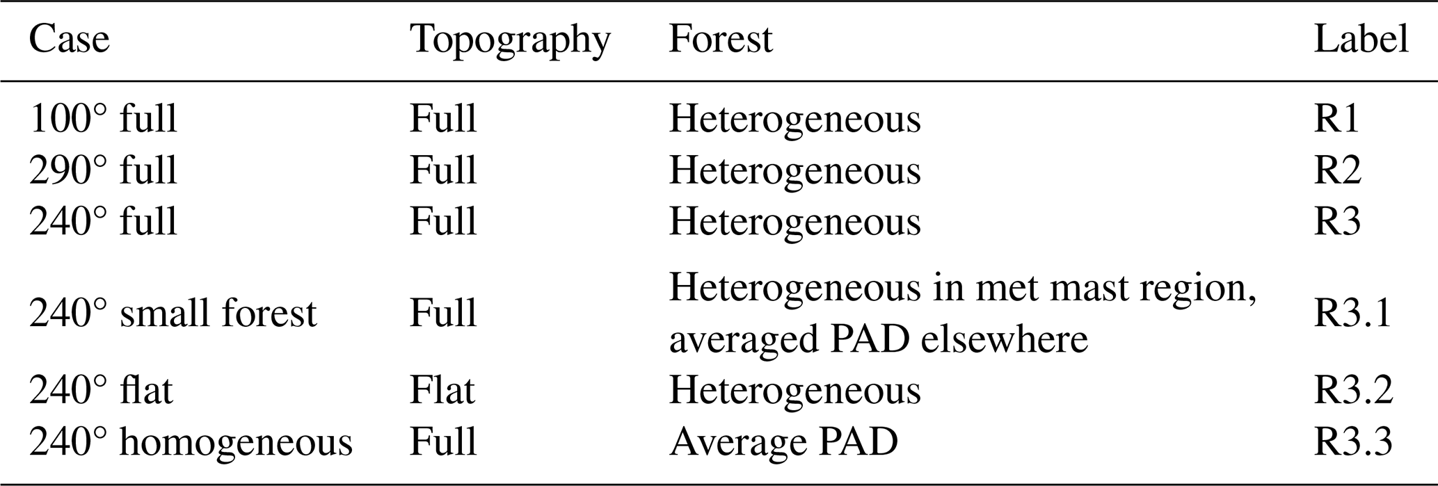
Figure 14 Wind profile (a) and wind shear exponent profile (b) from three wind directions for the tower position (Fig. 2). The lines represent the simulations in Table 3 and the reference case (F1 in Table 2). Measurements are indicated by the circles, with the estimation of 95 % statistical confidence for the mean value levels as error bars. The green-shaded area corresponds to forest height of 〈h_f2 m.

The wind speed and its shear, as represented by the shear exponent of the power law, are presented in Fig. 14. The wind speed is normalized with the 100 m TKE to facilitate comparison. From Fig. 14a it is clear that the LES overpredicts the normalized wind speed but that the relative differences between the directions follow the same trend as the measured wind profiles. It is also clear that case R3.3, which was made with realistic elevation but homogeneous forest (using the average forest density and height), overpredicts the normalized wind speed and underpredicts the shear. These results are in line with theoretical expectations regarding the impact of heterogeneity of surface roughness, which says that unevenly distributed surface roughness leads to a higher effective roughness than when spread out evenly (Bou-Zeid et al., 2004, 2020; Janzon et al., 2023). As expected, R3, R3.1, and R3.2 are very similar close to the forest. R3 and R3.1 start to diverge slightly at 30 m height, but the difference remains small for the entire profile. It is interesting that the wind profile for R3.1 has lower values than that of R3, while that of R3.3 has considerably higher values, since for most of the domain, R3.1 and R3.3 have the same constant PAD and tree height. The difference is rather local, and when the domain average wind speed is considered, both R3.1 and R3.3 show larger wind speed and lower TKE than R3, as reported in Table 4. The domain-averaged wind speed in R3.3 is 4.1 % larger at 100 m than in R3 and the resolved TKE 1.7 % lower, which again illustrates that neglecting heterogeneity in the PAD leads to an underestimation of the effective roughness.

Table 4 Relative differences in the domain-averaged quantities compared to simulation R3.

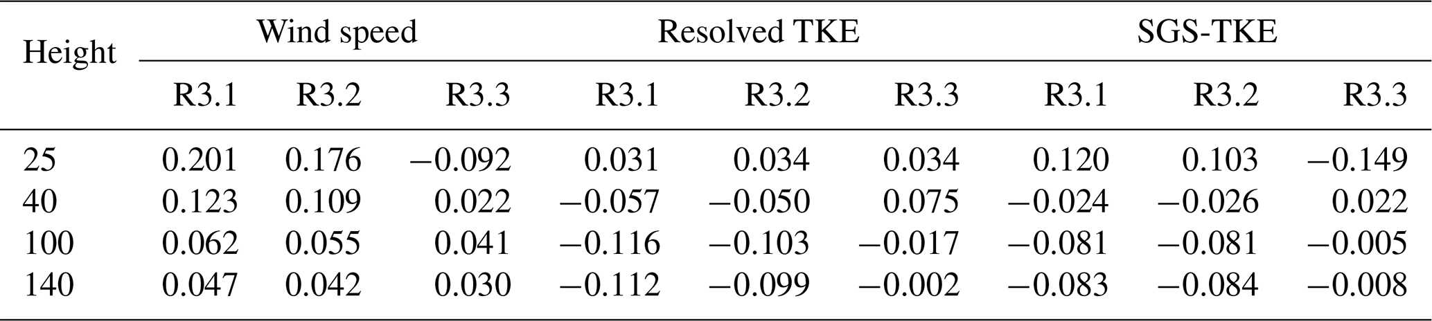
For the higher-order moments in Fig. 15, a notable observation is that the relatively coarse horizontal resolution of simulations R1–R3 has an impact on the anisotropy of the turbulence components. Relative to the measurements, the variance in u is overestimated, while it is underestimated for v and w. Above 5 〈h_f〉 the results agree better with the measurements. Case F1 employs a finer mesh that results in an anisotropy that better matches the observations below 5 〈h_f〉. For the shear stress, the resolution seems to have a smaller effect, and simulations R1–R3 match the observations relatively well, accurately predicting that the magnitudes in 290° fall more quickly with height than in 100 and 240°.

Figure 15 Second-order turbulence moments normalized by the turbulence kinetic energy at 100 m height. Variance in the mean wind direction (a), lateral variance (b), vertical variance (c), resolved TKE (d), and total shear stress (e). Estimates for the statistical 95 % confidence levels of the mean values for the measurements are shown by the error bars.

For the skewness of velocity components in Fig. 16, the most distinct feature is the peak associated with the forest top, displaying a positive pattern for u and negative for w, indicative of sweep-dominated mixing. Among the observations, which are only available at higher heights, the 290° shows the lowest values for the u component and the highest for the w component, indicating a slightly more ejection-dominated turbulence than for the other two directions. While the magnitudes are different in the simulations, the same trend is observed.

Figure 16 Skewness in the longitudinal, lateral, and vertical directions for the three wind directions at Ryningsnäs.

To further the discussion on the trade-off between sufficient upstream fetch and sufficient resolution, the simulations were also compared to observations in the frequency space. While it is evident that the anisotropy is poorly represented below 100 m (Fig. 15), it is clear from Fig. 17 that the low frequencies agree with measurements for all three velocity components and that it is the relatively large share of variance that resides at high frequencies for v and w that leads to the poor agreements at low heights. The lower variance of case F1 compared to R1, R2, and R3 is also clearly evident. While the lack of forest heterogeneity in F1 contributes to the lower variance, most of the discrepancy comes from a lower geostrophic wind forcing. When studying cross-spectral densities, even at relatively small vertical separations and at heights well below the hub heights of modern turbines (δ_z=18 m separation, 91 m centre height), the agreement between observations and simulations is approximately equal on all frequencies (Fig. 18). For larger vertical separations, 40 m (Fig. 19) and 100 m (Fig. 20), the general level of coherence matches between simulations and observations, as does the phase lag, which is clear only for the v component at 40 m separation but noticeable also for u at the larger separation. Note that the frequency axis is scaled for the two-point spectral statistics to facilitate comparison with the F1 case.

Figure 17 Power spectra of the longitudinal (a), lateral (b), and vertical (c) velocity components at the height of 98 m.

Figure 18 Vertical cross-spectra for δ_z=18 m separation of the longitudinal (a), lateral (b), and vertical (c) velocity components.

Figure 19 Coherence for δ_z≈40 m separation of the longitudinal (a), lateral (b), and vertical (c) velocity components and phase shifts for the longitudinal (d), lateral (e), and vertical (f) velocity components as a function of the normalized frequency.

Figure 20 Coherence for δ_z≈100 m separation of the longitudinal (a), lateral (b), and vertical (c) velocity components and phase shifts for the longitudinal (d), lateral (e), and vertical (f) velocity components as a function of the normalized frequency.

6.3 Footprint study

The focus is now placed on analyzing the impact of the forest modelling upstream of the met mast, specifically the significance of employing realistic forest conditions over an appropriate extension compared to using average forest values. The implications of using measured forest densities with all of their heterogeneity can clearly be seen in Fig. 14a and b, when focusing on the difference between cases R3 and R3.3. The topography on those simulations is identical, so the large difference in wind speed and shear is only due to the impact of the heterogeneity of the vegetation cover and density. The results agree with the findings of Bou-Zeid et al. (2004), Miller and Stoll (2013), and Janzon et al. (2023), which predict increasing effective roughness length with increasing surface roughness heterogeneity.

The R3.1 simulation was used to qualitatively assess the importance of using true vegetation cover in comparison with generic vegetation cover and the impact of limited upstream extent of true forest cover. Figure 21a and b shows the elevation and vegetation height of cases R3 and R3.1, whereas (c)–(f) shows the difference in normalized wind speed between the two simulations at heights 25, 40, 100, and 140 m above local ground, respectively. As expected, at 25 m height (just above the average forest height), the results reveal clear differences outside of the patch of equal PAD, while within the region of equal PAD, the wind speed is more alike, as illustrated by Fig. 21c. These variations are larger in regions devoid of trees in R3.0. At 40 m height, the patch of matching wind speeds moved slightly downstream, while the differences outside the region of equal PAD are smaller. At 100 m and above, however, the influence of the equal-PAD region is hardly distinguishable, and the maps are instead dominated by smaller differences in wind speed originating either from differences in upstream PAD or impact from random fluctuations due to low-frequency fluctuations.

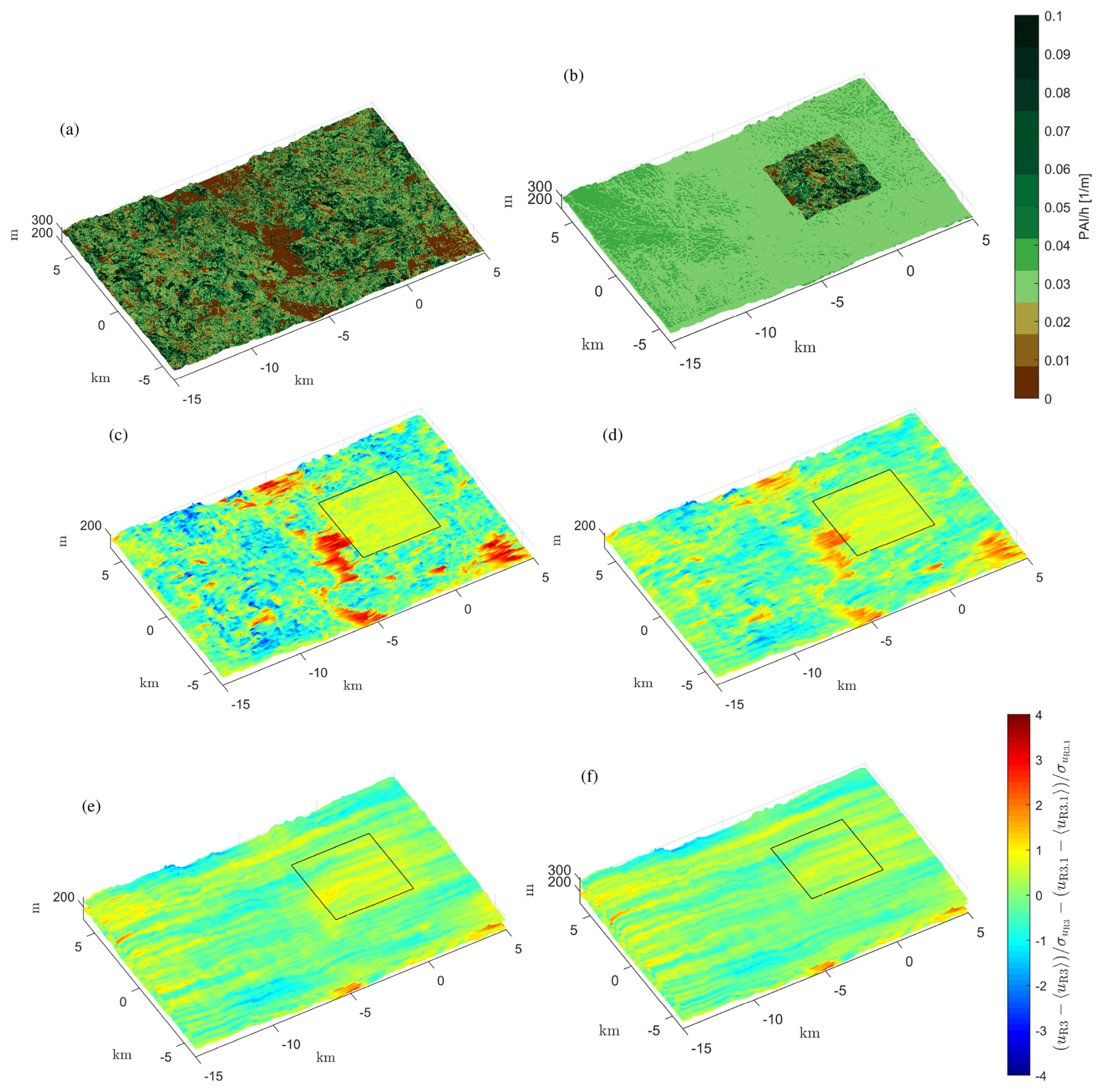
Figure 21 Vertically averaged PAD for runs R3 (a) and R3.1 (b). Difference between the normalized wind field fluctuations in cases R3 and R3.1 at heights 25 m (c), 40 m (d), 100 m (e), and 140 m (f) above local ground level. Note that the vertical axis is exaggerated. The black square has been added to indicate the part of the domain coinciding with the region of realistic forest conditions in R3.1.

The impact of the elevation-induced speedup was qualitatively assessed in the same fashion by comparing wind fields from simulations R3 and R3.2, which share the same realistic forest cover but where only R3 has realistic elevation and R3.2 is completely flat. The surface condition for R3.2 is shown in Fig. 22a, whereas the elevation of R3 is shown in Fig. 22b. When comparing normalized wind speeds above the local ground height for the two simulations, a speedup clearly appears that coincides with the terrain, as it is only present in R3 and not in R3.2. The speedup is most obvious at 40 and 100 m heights. At 20 m height, the pattern is dominated by small-scale variations stemming from small-scale terrain features, while at 140 m, those are filtered out, and only the larger terrain variations are visible in the speedup pattern. Even though the speedup pattern decreases in amplitude between 100 and 140 m above local ground, it is clear by comparing Figs. 22e and f to 21e and f that the pattern persists for much higher heights than the pattern linked to vegetation cover. It should be noted that a clear difference between the terrain-induced speedup pattern and the vegetation-linked pattern is that the former stays horizontally consistent with increasing height, while the latter is somewhat advected downstream with height.

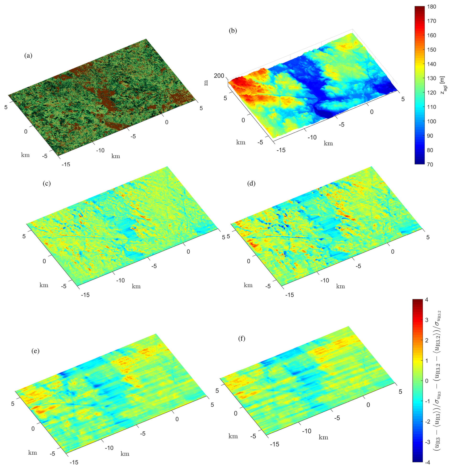
Figure 22 Surface conditions for runs R3.2 (a) and elevation in run R3 (b). Also, differences between the normalized wind field fluctuations in cases R3 and R3.2 at heights 25 m (c), 40 m (d), 100 m (e), and 140 m (f) above local ground level. Note that the vertical axis is exaggerated.

An extended perspective of the evolution of footprint with elevation is included in the Appendix. There, a comparison is made of the mean velocity and resolved and subgrid TKE from cases R3, R3.1, R3.2, and R3.3.

To quantitatively assess the requirements on domain size, the wind and TKE fields from simulations R1, R2, R3, and R3.2 were used. The wind fields where first normalized by removal of the mean and division by the standard deviation. The resulting fluctuations were then correlated with corresponding normalized fluctuations of surface drag, as measured by the magnitude of the vertical integral of Eq. (16). The correlation was made point-wise, starting with zero downstream separation and then varying the downstream separation while maintaining zero spanwise separation. The correlation was computed for all of the available two-point pairs within the inner region of uniform meshing (see Fig. 2), meaning that fewer pairs were available with larger downstream separation (due to the finite extension of the domain). The results were similar when keeping the number of pairs constant, but plots using the maximum number of pairs are displayed here to reduce scatter. The results are shown in Fig. 23. For wind field fluctuations, two effects are distinguishable. At low heights and for small separation distances, the correlation is negative and comes from the fact that higher, denser vegetation leads to a local reduction in wind speed due to drag. The maximum impact of this effect is seen at roughly 4–10 times downstream z_agl as judged by the results in Fig. 23g and j. The second effect is seen at higher heights above the ground and appears to be connected to speedup due to varying displacement height. The correlation is positive, indicating that locally, higher drag somewhat counterintuitively leads to a local increase in wind speed. This finding complements earlier footprint studies, which mainly focused on scalar fluxes at lower heights (Rannik et al., 2011), and highlights the importance of vertical displacements in environments with strong wind gradients. For the resolved TKE, an increase (decrease) in drag is associated with an increase (decrease) in TKE, with the maximum located approximately 10 z_agl downstream. An exception is seen at 25 m height, which at downstream distances smaller than 10 z_agl has negative correlation. It is unclear whether this should be attributed to a spurious correlation between wind speed and TKE or whether it has to do with the model's (in)ability to resolve small-scale TKE. The subgrid TKE consistently shows a positive correlation with drag, again with a maximum effect roughly 10 z_agl downstream. The results from each simulation in Table 3 display very similar behaviour, although it should be stressed that due to the terrain being flat in R3.2, this is the only case that is completely free of correlation between topography and forest height, and thus the results from R3.2 should be more representative of the impact of forest drag. These considerations lead back to the requirements of domain size. From the results, there are no indications of a correlation between wind speed and surface properties that would extend much more than 10 z_agl upstream. Conversely, the correlation with drag and turbulence comprises greater distances, at least up to 50 z_agl upstream for rotor-relevant heights. This will in turn have an impact on the local fluctuations and on the average wind speed.

Figure 23 Domain average of the two-point correlation between the magnitude of the local forest drag with the velocity (left column), the resolved TKE (middle column), and the subgrid TKE (right column) as a function of downstream separation between correlation pairs. The upper point in the correlation pair is at the height of 140 m (a, b, c), 100 m (d, e, f), 40 m (g, h, i), and 25 m (j, k, l), as indicated at the top left of each row. The lines follow the legend in Fig. 14.

6.4 Conclusions

This work has presented a methodology to simulate the wind field over forested regions that represent realistic conditions of topography and tree distribution. The methodology is based on LES, and it permits us to model the effect of the surface features on the turbulence characteristics of the flow. The surface characteristics comprise the representation of topography and, crucially, the explicit representation of forest by means of a plant area density (PAD) field so the drag on the wind flow is proportional to its local value and the flow velocity. The PAD and ground height can be determined through airborne laser scans, which has the great advantage that assumptions on roughness lengths and/or tree density profiles become much less important than in alternative approaches. The study has been divided into different parts whose conclusions are presented separately.

6.4.1 Verification

An extensive verification process has been shown, based on the simulation of idealized conditions comprising a homogeneous forest over flat terrain, which revealed the influence of various modelling choices on the flow characteristics. Attention was paid to three cases, two with different PADs and one with only ground roughness z₀ and displacement height d. The turbulence statistics and spectra showed general agreement with results found in the literature while also confirming that the turbulence field above the forest is different when the forest is explicitly modelled, in contrast to what is obtained when relying only on a wall model. Notably, higher streamwise skewness indicates a sweep-dominated mixing above the modelled canopy. The verification also highlights the problem of achieving high enough turbulence based solely on large values of z₀, as this requires a minimum height of the first cell node above the ground and away from the roughness sublayer to ensure the applicability of Monin–Obukhov (Basu and Lacser, 2017) while also maintaining a high cell resolution near this region. This problem does not appear when using PAD to model the forest drag. An important result of the verification is that in simulations employing PAD, the z₀ value did not impact the mean statistics at wind turbine heights. In other words, drag from the canopy completely dominates over drag from the surface, even when the PAD was set unrealistically low, showing no appreciable differences from when no wall model was used at all. The implication of this result is large, since on top of the issue with z₀ and the height of the first cell, PAD can be measured but z₀ cannot. Thus, using PAD eliminates the large uncertainty in estimating z₀ in the wind resource assessment, something that has been previously highlighted as an important challenge (Floors et al., 2018). An assessment of other modelling choices was also performed as part of the study. A significant result is that the flow characteristics at rotor heights were largely insensitive to the choice of subgrid-scale parameterization within the canopy, highlighting that the most important choice is between using a PAD field or not, whereas the details in the implementation of PAD drag only marginally impact the results at rotor heights, with changes being confined to the canopy level. An important omission from the study is the variability in C_D, which remains one of the largest uncertainties and weaknesses with the technique of explicit drag modelling. Attempts to quantify and parameterize C_D from field observations show large variations, in the range of 0.1 to above 1 (Yi, 2008; Bekkers et al., 2022). Given the magnitude of the variations, implementing a varying C_D value would potentially have a large effect, but it remains unclear what the cause of these variations are and hence how the effect should best be parameterized.

6.4.2 Validation

The methodology was validated by comparing the results of the simulation of wind flow over Ryningsnäs, a forested location with mild, complex terrain located in Sweden. To represent the actual surface conditions, the technique makes use of detailed forest density and topography maps to create a PAD field in the simulation domain and ground surface with a high degree of accuracy. Three incoming wind directions were considered when comparing the LES results with observations, showcasing some variation in topographic and forest distribution. The methodology was shown to be able to represent the relative differences in velocity and shear and TKE. However, the general magnitude of the TKE was slightly underestimated, and below 100 m the streamwise component had a positive bias, in contrast to the lateral and vertical components, an effect which is attributed to insufficient horizontal resolution, similar to Arnqvist et al. (2019). Vertically separated spectral statistics generally agreed with measurements over various separation distances and heights, but the scatter in the data did not permit us to show differences owing to the upstream fetch, for either the simulation or the observations. Spectral coherence from the IEC model predicted higher values than both the LES and the measurements for different separations δ_z as a function of the normalized frequency $f{\mathit{\delta }}_z/\stackrel{\mathrm{‾}}{u}$, a pattern that was also observed in the verification results under homogeneous forest conditions. While this result could suggest that the IEC model for spectral coherence might overestimate correlations outside the lowest frequencies under forested conditions, the cause could be more trivial. Indeed, if the velocity in the normalized frequency is not taken as the averaged value between the two locations as done here but a somewhat smaller value is used, the IEC curves would appear to shift toward smaller frequencies, providing a remarkable match to the LES results. To study what velocity would provide a better fit is left for future studies.

6.4.3 Capturing the footprint of the forest

Finally, a study of the footprint of the forest and topography was carried out with the aim of informing on the impact of surface conditions. The study examined the significance of representing forest heterogeneity by comparing results with those using a spatially uniform forest but identical topography. This showed that heterogeneous forest conditions not only produce a higher drag in comparison with homogeneous conditions, in agreement with prior studies (Bou-Zeid et al., 2020; Janzon et al., 2023), but also that accurately representing the forest indeed translates to better agreement with observations. Moreover, the simulation with flat ground lacked turbulence magnitude, but it should be noted that the studied site has low terrain complexity and that while realistic digital forest models may be difficult to acquire for all sites, realistic digital elevation models are much easier to find.

Two-point correlations agree with existing literature and initial assessments from surface-layer scaling arguments that most of the footprint for velocity is within 10 times the height of interest. For turbulence however, the footprint extended roughly five times longer. The simulations displayed typical elongated streamwise streaks, which is consistent with a longer upwind tail of the footprints than estimated from purely surface scales (Hutchins et al., 2012; Salesky and Anderson, 2020; Paleri et al., 2022). It should be emphasized that the simulations were run in strictly neutral conditions, and a simulation in stable conditions, where the turbulence intensity is much smaller, would have a significantly longer footprint due to reduced vertical mixing.

When comparing simulations using realistic forest in the entire domain to one where realistic forest is restricted to a small patch around the target location, the relative difference between the simulations showed no clear trace of the patch at a height above 100 m. The conclusion is that most of the difference is blended out and that remaining differences are seen only as spatial mean quantities. This supports the estimates of the blending height from Bou-Zeid et al. (2004), which are of the order of 100 m for clearing sizes and effective roughness lengths representative of this case. In contrast, the use of flat terrain in an otherwise identical representation of forest distribution indicated that differences observed in the wind field are more persistent with height. This is expected both because of terrain speedup effects and because streamlines are not entirely terrain following, which leads to higher (lower) wind speeds at hills (depressions) in the presence of a background wind shear.

6.4.4 Recommendations for site-specific wind modelling

The validation supports the notion that the effect of surface features on the flow is fairly well represented in the computations. In addition, it also shows that the limited resolution of the mesh plays a role in the prediction of the anisotropy of second-order quantities. The contrast between these findings offers the modeller two perspectives to weigh when it is desired to capture the footprint of the surface on the wind over long distances in order to reproduce the wind characteristics seen at heights covered by the rotor area of a wind turbine. Other than single-point anisotropy levels at low heights, no clear drawbacks were found from the relatively low resolution, and since wind turbines will act as considerable spatial filters for turbulence, to employ domains that cover a sufficiently long region upstream of the met mast seems to be of greater importance compared to the refinement of the mesh, particularly in the horizontal direction.

The majority of the footprint for wind speed is located within 10 times the height of interest downstream, but it is longer for turbulence. Since the effects of drag are both advected downstream and diffused by turbulence, the footprint is expected to be longer and narrower for stable conditions and sites with lower effective roughness. Missing heterogeneity in PAD leads to underestimation of the effective roughness, but using full heterogeneity only in the footprint did not increase the error relative to observations.

The simulations were made using periodic boundary conditions, which necessitate evening out the terrain at the edges of the domain. This should be considered when estimating the requirements on domain size since edge effects also advect and diffuse in the same manner downstream. Subsequently, if the manipulation of the terrain is large at the edges of the domain, an adjustment region before the footprint area should be included.

Finally, the most clear result was that using explicit forest drag instead of roughness and displacement makes the simulation less subjective and solves the problem of large z₀ relative to the first cell node z₁. The impacts of particular choices in how to implement explicit drag were small compared to not using explicit drag at all.

6.4.5 Directions for further research

All the simulations were made using strictly neutral conditions, and the most obvious direction is to investigate the impact of atmospheric stratification. This will influence the extent of the footprint but also change the effect of surface topography. How to treat the side boundary conditions have also been left out of this study, and an interesting question is whether periodic boundary conditions are still viable when the terrain complexity is larger and if transient thermodynamic and pressure gradient forcing will be applied. While the PAD data certainly appear realistic, the effective roughness was slightly lower than for the tower observations. It remains an open question if this is due to a misrepresentation of PAD by the ALS-conversion technique, a resolution issue (in either PAD or the LES mesh) or if the problem is the treatment of the drag coefficient (either the magnitude or the use of a constant value).

Appendix A

The following figures are shown to complement the view of the evolution of footprint discussed in Sect. 6.3. These provide a comparison of horizontal planes of mean velocity in Fig. A1, resolved TKE in Fig. A2, and subgrid TKE in Fig. A3, obtained 25, 40, 100, and 140 m above ground from setups R3, R3.1, R3.2, and R3.3 described in Sect. 4.2.3 and Table 3.

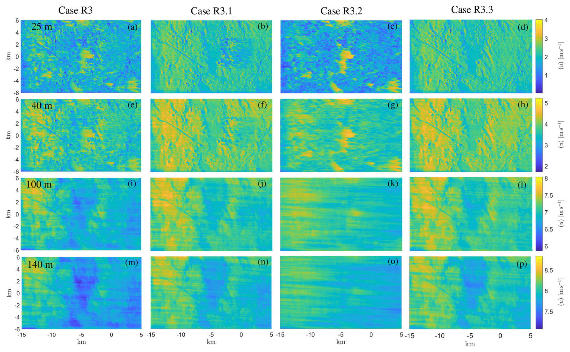
Figure A1 Temporal mean velocity fields at heights 25 m above local ground (a–d), 40 m above local ground (e–h), 100 m above local ground (j–l), and 140 m above local ground (m–p). Column 1 (a, e, i, m) is from simulation R3, Column 2 (b, f, j, n) is from simulation R3.1, Column 3 (c, g, k, o) is from simulation R3.2, and Column 4 (d, h, l, p) is from simulation R3.3. Note that the scales vary for different elevations to highlight the features of the spatial distribution.

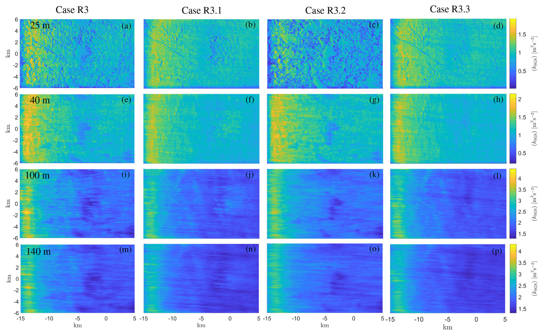
Figure A2 Temporal mean fields of the resolved TKE at heights 25 m above local ground (a–d), 40 m above local ground (e–h), 100 m above local ground (j–l), and 140 m above local ground (m–p). Column 1 (a, e, i, m) is from simulation R3, Column 2 (b, f, j, n) is from simulation R3.1, Column 3 (c, g, k, o) is from simulation R3.2, and Column 4 (d, h, l, p) is from simulation R3.3. Note that the scales vary for different elevations to highlight the features of the spatial distribution.

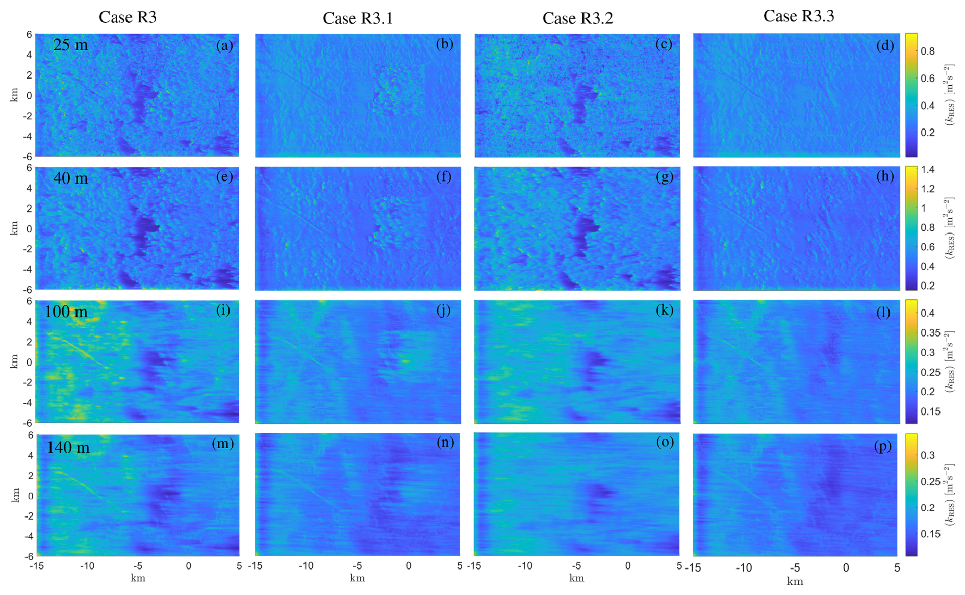
Figure A3 Temporal mean fields of the SGS-TKE at heights 25 m above local ground (a–d), 40 m above local ground (e–h), 100 m above local ground (j–l), and 140 m above local ground (m–p). Column 1 (a, e, i, m) is from simulation R3, Column 2 (b, f, j, n) is from simulation R3.1, Column 3 (c, g, k, o) is from simulation R3.2, and Column 4 (d, h, l, p) is from simulation R3.3. Note that the scales vary for different elevations to highlight the features of the spatial distribution.