Annual wake impacts in and between wind farm clusters – Part 1: WRF-simulated wake losses for different atmospheric conditions

With the rapid increase in wind farm developments, it is essential to evaluate the impacts of newly constructed wind farms on adjacent wind farms, both existing and planned. Numerical weather prediction models are essential tools to predict wake effects, especially under varying atmospheric conditions that occur throughout the year. In this study, we investigate the annual variation in wake effects caused by the planned Belgian Princess Elisabeth (PE) wind farm cluster on adjacent, existing wind farms in the southern North Sea. To represent the annual effect, a representative year is simulated with the Weather Research and Forecasting (WRF) model. The analysis focuses on how variability in atmospheric conditions influences wake interactions throughout the year, which is important for wind farm planning and operational strategies. A distinction is made between external wake energy losses, caused by the new wind farm cluster, and internal wake energy losses, caused by the individual wind farms within the existing area. The diurnal variations in external wake energy losses are driven by changes in atmospheric stability, while the seasonal variations are largely a consequence of seasonal variations in wind direction, wind speed, and atmospheric stability. In contrast, internal wake energy losses are mainly determined by seasonal patterns and show only weak diurnal variability. The spatiotemporally averaged external wake energy losses are limited to 4 %, while the internal wake energy losses can reach 42 % for the closest adjacent BE–NL wind farm. The spatial distribution of wake losses further reveals that turbines located in the center of a wind farm experience higher internal wake energy losses, especially in densely packed layouts, while those at the edges are less affected for internal wake energy losses but more for external wake energy losses. Both the internal and external energy losses decrease with increasing atmospheric instability when wind speeds are in Region II of the wind turbine's power curve, where wind turbine operation maximizes the power coefficient. When binning for wind speed and wind direction, stable stratification results in external wake energy losses that are approximately twice as large as in unstable stratification. The presence of the new wind farm cluster also leads to episodes of negative wake energy losses, implying power gain after the construction of the PE wind farm cluster, which are related to flow speedup around the new wind farm. This paper constitutes Part 1 of a two-part study. In Part 2 (Porchetta et al., 2026), the impacts induced by the PE wind farm cluster are evaluated using fast-running engineering wake models and compared against the WRF results presented here, allowing for a systematic assessment of differences and uncertainties between models.

1 Introduction

Wind energy holds significant potential as a primary contributor to meet the growing demand for renewable energy production in the global community, with the expectation that wind energy will account for up to one-third of the global energy supply by 2050 (Veers et al., 2019). Following the signing of the Ostend Declaration in April 2023, Belgium, Germany, Denmark, and the Netherlands have committed to delivering 65 GW of offshore wind by 2030, illustrating the exponential growth that one can expect in development areas such as the North Sea. As the deployment of wind farms continues to accelerate, leading to smaller distances in between wind farms, it becomes crucial to investigate interactions between neighboring wind farms. Wind farms create wakes, which are regions of mean momentum and mean kinetic energy deficit downwind of the turbines (Fischereit et al., 2022b). These wakes can extend over large distances (Platis et al., 2018; Schneemann et al., 2020) and influence the power production of downwind wind farms (Lundquist et al., 2019; Barthelmie et al., 2010; Pryor et al., 2021; Stieren and Stevens, 2022).

A variety of numerical models have been employed to examine these farm–farm wakes. Recently, studying wakes within a mesoscale (or numerical weather prediction) model framework has gained prominence (Cuevas-Figueroa et al., 2022). Mesoscale models are particularly valuable for their ability to incorporate the influence of multiple atmospheric variables, which may exhibit non-uniform spatial and temporal distributions. However, it is important to note that typical horizontal resolutions in mesoscale models for wind energy research mostly range from 1 to 3 km, which is larger than the spacing between the wind turbines (Fischereit et al., 2022a). However, horizontal resolutions may also be as fine as 333 m or as coarse as 5 km (Prosper et al., 2019).

To account for subgrid-scale effects of wind turbines, which are not explicitly resolved by the model, wind farm parameterizations are employed within mesoscale models (Veers et al., 2019). Here, wind turbines are typically parameterized as a momentum sink and turbulence kinetic energy source within the planetary boundary layer. A widely used scheme is the Fitch parameterization (Fitch et al., 2012), which represents the extracted momentum by a single wind turbine based on the turbine thrust curve, and the added turbulent kinetic energy (TKE) is proportional to the difference between the thrust and power coefficients. This allows the model to account for both the wake velocity deficit and the enhanced mixing caused by turbine-induced turbulence. Other wind farm parameterizations focus on further elaborating on this parameterization by tuning model coefficients or incorporating additional physical effects such as wind shear and turbine layout (Redfern et al., 2019; Pan and Archer, 2018). Over the years, these different wind farm parameterizations have been developed and implemented in mesoscale models to investigate a wide range of questions. These investigations, employing different wind farm parameterizations, have included studying the effects of wind veer and shear using the rotor equivalent wind speed model (Redfern et al., 2019), wind waves and swell (Porchetta et al., 2021), wind farm layout (Pan and Archer, 2018), and model resolution (Pryor et al., 2020), among others, on the power production and wakes of wind turbines.

Until recently, mesoscale wake studies have predominantly focused on limited time periods that are insufficient to directly assess annual mean wake effects or sub-annual wake variability. These shorter time periods were often chosen because of the high computational cost associated with long-term simulations. However, with increasing computational resources, it is becoming more common to perform simulations over full years or longer (Palatos-Plexidas et al., 2025). Earlier studies approached seasonal variability by using representative subsets of data. Pryor et al. (2021) investigated eleven 5 d periods in order to represent seasonality. A similar approach was used by Fischereit et al. (2020), where 180 d was selected to represent the wind and wave climate to investigate the wind–wave–wake interactions of wind farms in the North Sea. More recently Borgers et al. (2024) investigated farm–farm wakes for 1 year for different wind farm density scenarios for planned wind farm locations in the North Sea. Their findings revealed that farm–farm wakes are highly sensitive to capacity density, inter-farm spacing, and wind farm sizes. In addition, Akhtar et al. (2021) simulated the wake impacts in the North Sea over multiple years; however, both Akhtar et al. (2021) and Borgers et al. (2024) employed similar wind turbines over the full area and did not account for the actual type of installed/planned wind turbines. These theoretical studies can provide useful insight into the importance of farm–farm interactions but are less relevant to quantify the effect of future planned wind farm clusters on the actual adjacent existing wind farms, as these studies do not consider the actual wind farm characteristics. In contrast, Cuevas-Figueroa et al. (2022) investigated farm–farm interaction of an operational farm for shorter periods of time and stated that yearly runs are still computationally expensive. Borgers et al. (2025) simulated a realistic 92 GW North Sea wind farm expansion scenario with COSMO-CLM and found that inter-farm wakes could reduce annual energy production by more than 10 % at several sites, with the Princess Elisabeth zone causing power reductions exceeding 15 % during certain high-wind 24 h periods. Lastly, Rosencrans et al. (2024) studied the sub-annual variability in offshore wind deployments in the mid-Atlantic and observed monthly and daily fluctuations in power deficits resulting from farm–farm interactions. They also showed the non-negligible effect of farm–farm interactions. It is clear that there is a growing interest in farm–farm interactions in numerical weather prediction models for periods that resolve seasonal variations.

This study investigates annually averaged wake effects and sub-annual wake variability in a newly planned wind farm cluster on adjacent existing wind farms. These effects are predicted using the Weather Research and Forecasting (WRF) model (Skamarock et al., 2008). More specifically, the effect of the new Princess Elisabeth (PE) wind farm cluster, which will be built in the near future in the Belgian part of the North Sea, is investigated. A year is simulated in which the annual wind climate is very similar to the wind climate of 1990–2020, allowing the most typical wake effects on the existing neighboring wind farms to be examined. The present study thus focuses on representative present-day atmospheric conditions, and potential changes in offshore wind climate under future climate scenarios are outside the scope of this work. Furthermore, this study focuses solely on the most commonly used wind farm parameterization despite the knowledge that certain parameterizations perform better under specific conditions. The primary objective of this study is to offer insights into the annual wake impact and its sub-annual variability for one of the main offshore wind energy development hotspots, using the most commonly employed, out-of-the-box wind farm parameterization within WRF. The determinants of the wind farm wake effects on neighboring wind farms are quantified by considering wind speed, wind direction, and atmospheric stability over an annual period.

This paper constitutes Part 1 of a two-part study investigating wake impacts of an offshore wind farm cluster. In Part 2 (Porchetta et al., 2026), the wake impacts induced by the Princess Elisabeth wind farm cluster are evaluated using fast-running engineering wake models and compared against the numerical weather prediction results presented here, allowing for a systematic assessment of model approach differences and uncertainty in long-term farm–farm wake estimates.

2 Material and methods

The materials and methods presented in this section are applied to the new Princess Elisabeth (PE) wind farm cluster and existing adjacent wind farms. The same methodology can be extrapolated to study other farm–farm interactions.

2.1 Study area and period

Within the southern portion of the North Sea, a new wind farm cluster, the Princess Elisabeth cluster (PE) (red dots in Fig. 1), will be built. Although the final installed capacity is still under discussion, ranging from 3.15 to 3.5 GW, only one possible wind farm scenario is considered in this study, corresponding to a newly installed capacity of 3.5 GW with 15 MW turbines with a rotor diameter of D=236 m and a hub height of z_h=146 m (Munters et al., 2022). While the impact of the new wind farm cluster on all neighboring farms is investigated, the Belgian–Dutch (BE–NL) wind farm cluster, located just downstream of the prevailing southwesterly wind direction, is the primary focus of this study. However, as other nearby wind farms are likely to be affected (Lundquist et al., 2019; Barthelmie et al., 2010; Pryor et al., 2021; Stieren and Stevens, 2022), they are also considered in the numerical weather prediction model of this study (Fig. 1, Appendix A). In total, the influence of the Princess Elisabeth wind farm zone on 1409 wind turbines is investigated. The turbines are modeled in the numerical simulations with the appropriate turbine manufacturer curves or approximations thereof (Pierrot, 2024; EMD International A/S, 2024). The locations of the existing wind turbines are extracted from Hoeser et al. (2022), while the locations for the new Princess Elisabeth wind farm are from Munters et al. (2022) and Cornillie et al. (2021). The latter layout results from a preliminary distribution of turbines over the lease area, accounting for a known exclusion zone, without delving into the specifics of micrositing based on sea surface topography.

The simulations are performed for the year 2016 as it is a representative year for the long-term wind climate at 100 m above mean sea level for the study area. This was determined based on the methodology outlined in Borgers et al. (2024), based on hourly ERA5 data for the period 1990–2020 (Appendix B). This methodology identifies a representative year by comparing the wind speed and wind direction distributions for a single year with the long-term distributions. Other parameters, such as atmospheric stability and wave conditions, were not explicitly considered and could be included in future work. The goal of using a representative year is so that this study can provide an appropriate basis for long-term representation of the influence of building the new Princess Elisabeth wind farm cluster close to neighboring wind farms.

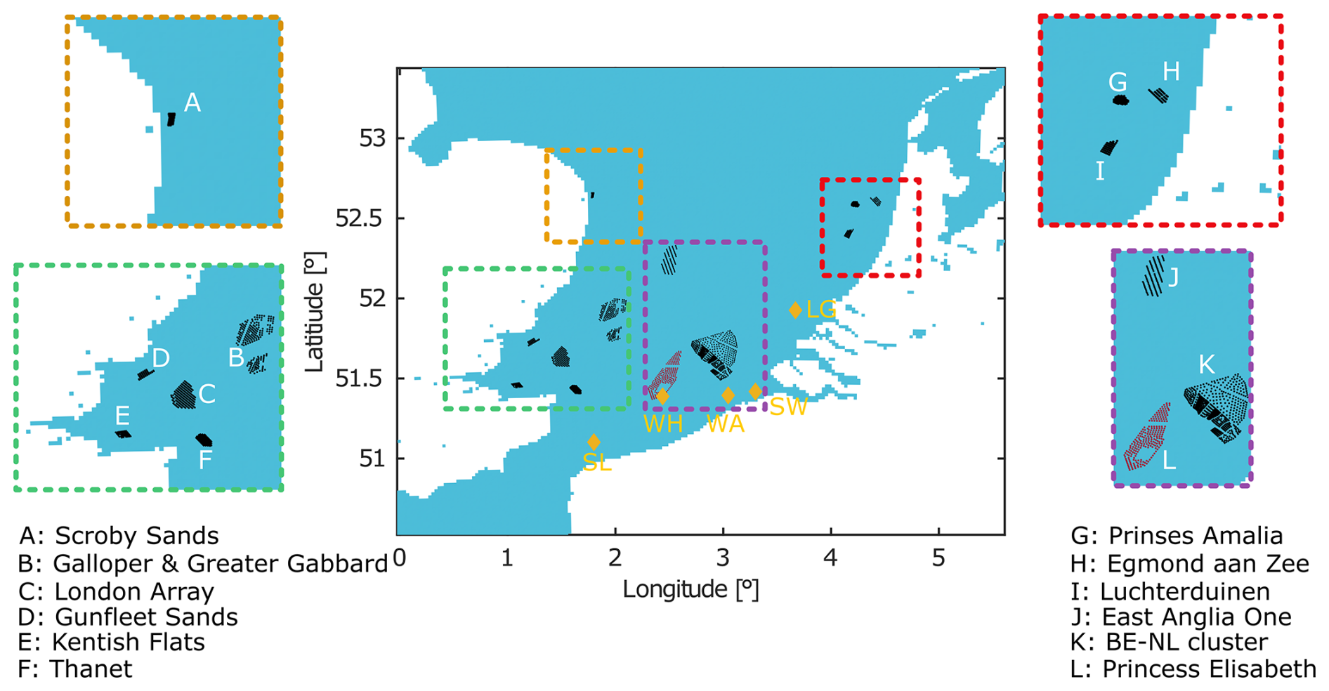
Figure 1 Location of the new Princess Elisabeth wind farms (red dots) and the existing wind farms (black dots) within the southern North Sea. Yellow diamonds show the location of measurement masts, with further details found in Table 1.

2.2 Observation stations

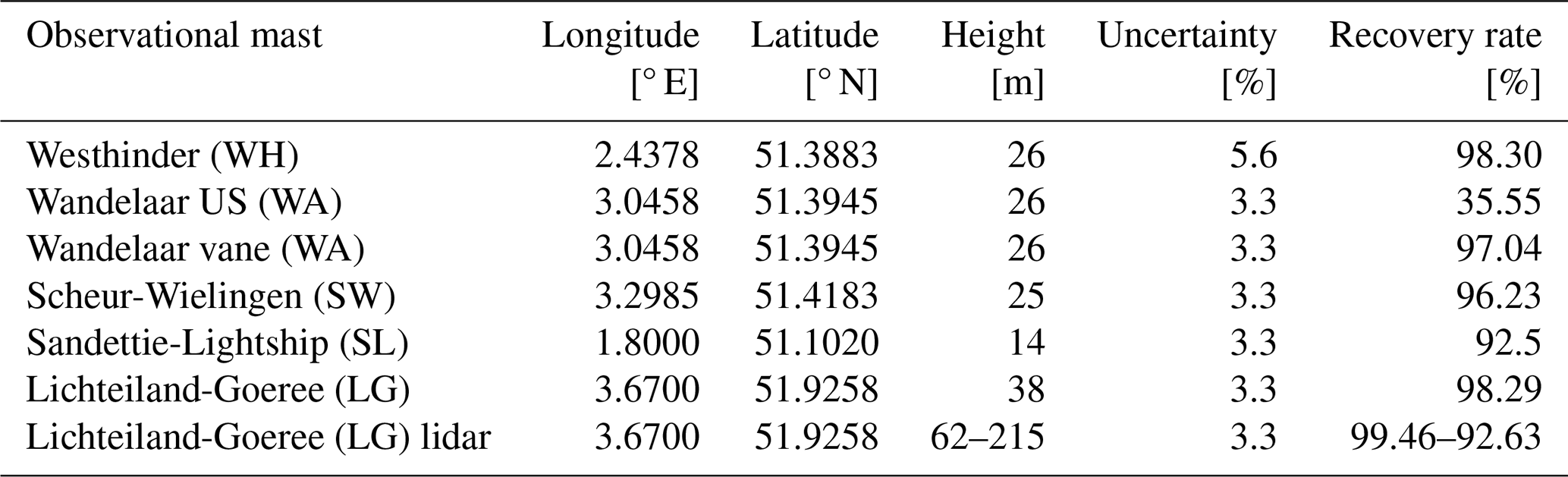
The simulation results are compared with offshore measurements. For the year 2016, five measurement platforms (yellow diamonds Fig. 1, Table 1) measured wind speed and wind directions at different altitudes and with a temporal resolution of 10 min (Borgers et al., 2024). These measurements were taken by boom- or platform-mounted anemometers, wind vanes, or a lidar. At the location of Wandelaar (WA) both anemometers and vanes are present, while at Lichteiland-Goeree (LG) both an anemometer and a lidar are present. Table 1 also shows the uncertainty in the wind speed measurements, including the uncertainty in the calibration, mounting, data acquisition, and local site conditions (Borgers et al., 2024). For wind direction the measurement uncertainty is not known. Furthermore, Table 1 indicates the recovery rate at each observational mast, representing the percentage of available measurements relative to the total expected measurements during 2016.

Table 1 Observational mast name, location, measurement altitude, uncertainty in the wind speed measurements, and recovery rate for 2016.

2.3 Mesoscale model setup

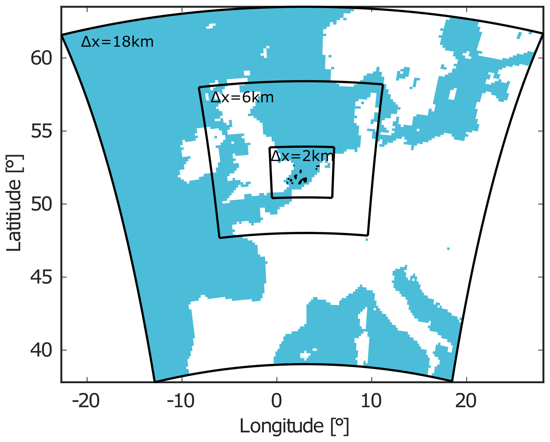
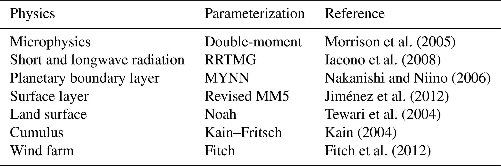
The numerical model used is the Weather Research and Forecasting (WRF) model v4.3 (Skamarock et al., 2008) with three nested domains (150 × 150, 190 × 190, and 220 × 190 grid cells) with a horizontal grid spacing of 18 km for the outermost domain, 6 km for the middle domain, and 2 km for the innermost domain (Fig. 2) following the recommendation of Fischereit et al. (2022a). The vertical resolution has 80 vertical levels that are stretched, resulting in more levels close to the surface, following the recommendations of Lee and Lundquist (2017). Within the first 150 m there are approximately 15 vertical levels. The model top is located at 1000 Pa. The Global Multi-resolution Terrain Elevation Data (GMTED2010) is imposed for the geographical data with a resolution of 30 arcsec. The initial and lateral boundary conditions come from the ERA5 reanalysis data set provided by the European Centre for Medium-Range Weather Forecasts (Hersbach et al., 2023a, b), which has a 0.25° × 0.25° horizontal grid resolution, 1 h temporal resolution, and 37 pressure levels up to 1 hPa. The physical parameterizations in this study are based on previous studies for similar applications in the same geographical region (Table 2) (Siedersleben et al., 2020; Porchetta et al., 2020, 2021). The parameterizations are a double-moment microphysics scheme (Morrison et al., 2005), the long- and shortwave Rapid Radiative Transfer Model for General Circulation Models (RRTMG) (Iacono et al., 2008), the revised MM5 surface layer scheme (Jiménez et al., 2012), the Noah land surface scheme (Tewari et al., 2004), the Kain–Fritsch cumulus scheme (Kain, 2004) (only applied to the parent domain as the two innermost domains have a convective permitting resolution), and the Mellor–Yamada Nakanishi Ninno (MYNN) planetary boundary layer scheme (Nakanishi and Niino, 2006). The simulations were performed using the atmospheric WRF model in a stand-alone configuration without explicit coupling to an ocean or wave model (e.g., ROMS, SWAN, or WAM). When wind turbines are included, the parameterization of Fitch et al. (2012) is used with a turbulent kinetic energy generation parameter of 0.25, which currently is the default value used in WRF (Archer et al., 2020).

Figure 2 The WRF computational configuration with three nested domains with a horizontal grid spacing of 18, 6, and 2 km for the outer to the innermost domain. The innermost domain shows all wind farm clusters included in the simulations (see Fig. 1 and Table 1 for details).

Morrison et al. (2005)Iacono et al. (2008)Nakanishi and Niino (2006)Jiménez et al. (2012)Tewari et al. (2004)Kain (2004)Fitch et al. (2012)

Table 2 Parameterizations used in the WRF simulations.

Three simulations for the year 2016 are performed: a first one where no wind farms are included, which is used as a reference simulation; one simulation with only the existing wind farms in 2022 (black dots, Fig. 1; see Appendix A); and one simulation with the existing wind farms in 2022 and the new Princess Elisabeth wind farm cluster (black and red dots, Fig. 1). The names of these three simulations throughout the paper are referred to as “no WF”, “without PE”, and “with PE”, respectively. The simulations including wind turbines (without PE and with PE) have exactly the same setup as the no-WF setup, grid size, and employed parameterizations except for the additional wind farm parameterization.

2.4 Stability classification

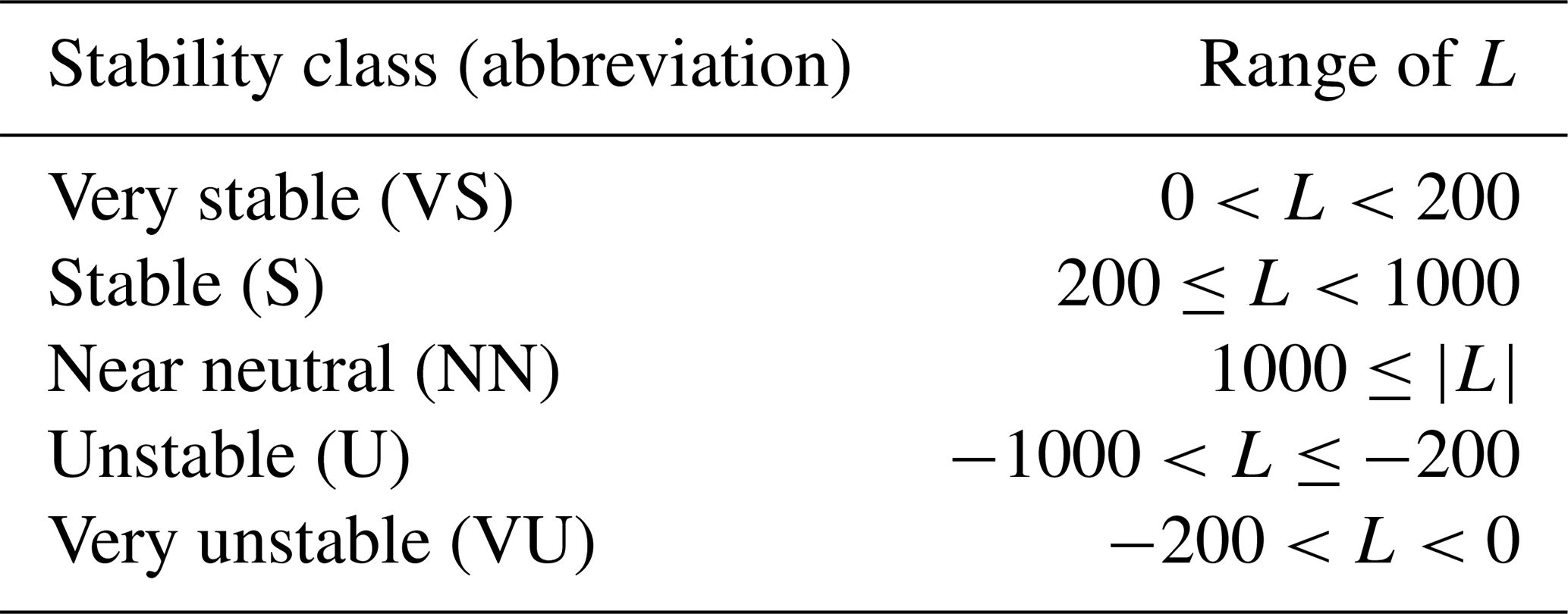
Because atmospheric stability has significant effects on the wakes of wind turbines (Platis et al., 2022; Rosencrans et al., 2024; Wu et al., 2023), it is important to investigate how the wake impacts of the new PE wind farm are influenced by different atmospheric stability regimes. The atmospheric stability in this work is defined by the Monin–Obukhov length (L), which categorizes atmospheric stability based on the ratio of turbulence production by mechanical shear to turbulence production by buoyancy associated with the surface layer (Monin and Obukhov, 1954). The different stability classes based on L are shown in Table 3. This classification is proposed by Van Wijk et al. (1990) and has been utilized in various studies (Porchetta et al., 2019; Nybø et al., 2020; Platis et al., 2022; Howland et al., 2022). The Monin–Obukhov length is output in 10 min intervals by WRF and is calculated by the surface layer scheme (Jiménez et al., 2012). A stability classification based on the bulk Richardson number between model levels at 10 and 100 m produced similar results, showing a Pearson correlation of 72 % with the Monin–Obukhov length classification. Consequently, only the Monin–Obukhov length method is applied in the following analyzes.

Table 3 Atmospheric stability classification based on the Monin–Obukhov length (L).

2.5 External and internal wake energy loss quantification

In this study, we quantify the total wake energy losses and decompose them into internal and external contributions. External wake energy losses are defined as the additional wake-induced energy losses caused by the new PE wind farm cluster on the existing wind farms. Internal wake energy losses, as defined here, represent the wake energy losses experienced by the existing wind farms in the absence of the PE wind farm cluster. It is important to note that this definition differs from the strict definition of internal wake energy losses, which includes only wake effects generated by turbines within the same wind farm. Due to the simulation setup employed in this study, this distinction cannot be made. Consequently, the internal wake energy losses presented here include inter-farm wake effects among the existing wind farms but exclude wake effects originating from the new PE wind farm cluster. Note that the internal wake effects of the Belgian–Dutch cluster virtually exclusively originate from wind turbines within the dense cluster, as other wind farms included in the without-PE simulation are at least 58 km away.

Three different averaging procedures are employed, where N_s is the number of turbines, N_t the number of time steps, and P_i(t) the instantaneous power output of turbines within grid cell i at time t.

• Temporal average: ${\stackrel{\mathrm{‾}}{P}}_i=\frac{\mathrm{1}}{N_{\mathrm{t}}}{\sum }_{t=\mathrm{1}}^{N_{\mathrm{t}}}{P}_i\left(t\right)$, i.e., the average over time for turbine-containing grid cells

• Spatiotemporal average: $\stackrel{\mathrm{‾}}{P}=\frac{\mathrm{1}}{N_s{N}_{\mathrm{t}}}{\sum }_{i=\mathrm{1}}^{N_s}{\sum }_{t=\mathrm{1}}^{N_{\mathrm{t}}}{P}_i\left(t\right)$, i.e., averaging across all turbine(s) containing grid cells and time steps simultaneously

• Spatiotemporal conditional average: ${\stackrel{\mathrm{‾}}{P}}_{\text{spatio-bin}}=\frac{\mathrm{1}}{N_{\mathrm{bin}}}{\sum }_{i,t\in \mathrm{bin}}{P}_i\left(t\right)$, considering only specific conditions such as wind speed, wind direction, atmospheric stability, or a combination of the previous

The absolute internal wake energy loss is defined in Eq. (1) as the power reduction of the reference power (no WF) associated with the existing wind farms only (without PE). The reference power ${\stackrel{\mathrm{‾}}{P}}_{\text{no WF}}$ is obtained by sampling the hub height wind speed from the no-WF WRF simulation at each turbine location and converting it to power using the turbine power curves. The total (internal + external) absolute wake energy loss is defined in Eq. (2) as the difference between the reference power and the mean power obtained in the presence of both the existing wind farms and the PE cluster (with PE). The absolute external wake energy loss induced by the PE wind farm cluster is defined in Eq. (3) as the difference between the total and internal losses:

$$\begin{array}{}\text{(1)}& {\displaystyle }\mathrm{\Delta }{\stackrel{\mathrm{‾}}{P}}_{\mathrm{internal}}={\stackrel{\mathrm{‾}}{P}}_{\text{no WF}}-{\stackrel{\mathrm{‾}}{P}}_{\text{without PE}},\text{(2)}& {\displaystyle }\mathrm{\Delta }{\stackrel{\mathrm{‾}}{P}}_{\mathrm{internal}+\mathrm{external}}={\stackrel{\mathrm{‾}}{P}}_{\text{no WF}}-{\stackrel{\mathrm{‾}}{P}}_{\text{with PE}},\text{(3)}& {\displaystyle }\begin{array}{rl}\mathrm{\Delta }{\stackrel{\mathrm{‾}}{P}}_{\mathrm{external}}& =\mathrm{\Delta }{\stackrel{\mathrm{‾}}{P}}_{\mathrm{internal}+\mathrm{external}}-\mathrm{\Delta }{\stackrel{\mathrm{‾}}{P}}_{\mathrm{internal}}\\ & ={\stackrel{\mathrm{‾}}{P}}_{\text{without PE}}-{\stackrel{\mathrm{‾}}{P}}_{\text{with PE}}.\end{array}\end{array}$$

From the absolute wake energy losses defined in Eqs. (1)–(3), the corresponding percentage wake energy losses are obtained by normalization with the reference power ${\stackrel{\mathrm{‾}}{P}}_{\text{no WF}}$. The percentage internal wake energy loss is defined in Eq. (4) as the relative power reduction associated with the existing wind farms only (without PE), normalized by the reference power. The total (internal + external) percentage wake energy loss is defined in Eq. (5) as the relative power reduction in the presence of both the existing wind farms and the PE cluster (with PE), normalized by the reference power. The percentage external wake energy loss induced by the PE wind farm cluster is defined in Eq. (6) as the difference between the total and internal percentage losses:

$$\begin{array}{}\text{(4)}& {\displaystyle }{\text{Loss}}_{\mathrm{internal}}=\mathrm{100}\times {\displaystyle \frac{\mathrm{\Delta }{\stackrel{\mathrm{‾}}{P}}_{\mathrm{internal}}}{{\stackrel{\mathrm{‾}}{P}}_{\text{no WF}}}},\text{(5)}& {\displaystyle }{\text{Loss}}_{\mathrm{internal}+\mathrm{external}}=\mathrm{100}\times {\displaystyle \frac{\mathrm{\Delta }{\stackrel{\mathrm{‾}}{P}}_{\mathrm{internal}+\mathrm{external}}}{{\stackrel{\mathrm{‾}}{P}}_{\text{no WF}}}},\text{(6)}& {\displaystyle }{\text{Loss}}_{\mathrm{external}}=\mathrm{100}\times {\displaystyle \frac{\mathrm{\Delta }{\stackrel{\mathrm{‾}}{P}}_{\mathrm{external}}}{{\stackrel{\mathrm{‾}}{P}}_{\text{no WF}}}}.\end{array}$$

All (absolute or percentage) wake energy losses are computed from the averaged power values defined above, rather than from instantaneous (absolute or percentage) losses at individual time steps. As described earlier, these losses (internal, external, and total) are analyzed using temporal, spatiotemporal, and spatiotemporal conditional averages to further elucidate the drivers of the interactions between turbines and farms. Throughout this paper, the term wake energy losses refers to the percentage definitions given in Eqs. (4)–(6), unless explicitly stated as absolute wake energy losses, in which case the definitions of Eqs. (1)–(3) are used.

In addition to wake energy loss metrics, annual energy production (AEP) is computed by integrating the power of the turbines over the full simulation period. AEP is calculated separately for the without-PE and with-PE simulations, and AEP losses are reported as a relative change between these two cases. In contrast to the wake energy loss definitions above, AEP changes are normalized by the baseline production of the existing wind farms, without PE, rather than by the no-WF reference.

3 Results and discussion

Throughout this paper, the results are shown on grid cells, which refer to single horizontal WRF model grid cells. As multiple turbines may fall within one grid cell, all wind farm quantities evaluated at the grid cell level (e.g., power or wake energy losses) represent aggregated model responses rather than turbine-resolved values.

3.1 WRF validation

The performance of the WRF model representation of the wind field is first evaluated. The simulations in this study represent idealized scenarios, as only a few of the Belgian–Dutch wind farms (Thorntonbank I, II, and III; Belwind; and Northwind; 182 of 572 turbines) were operational in 2016, while the existing turbines used in the simulations correspond to the wind farm layout as of 2022. However, the year 2016 is selected because it is identified as the most meteorologically representative. As a consequence of this mismatch between the meteorological year and the wind farm layout, a true validation of wake energy losses is not possible. As such, validation will only become feasible once post-construction field observations for the fully developed wind farm area become available (Palatos-Plexidas et al., 2025). Future research may then also explore the optimal representation of the wind field by selecting the most appropriate model configuration and parameterizations.

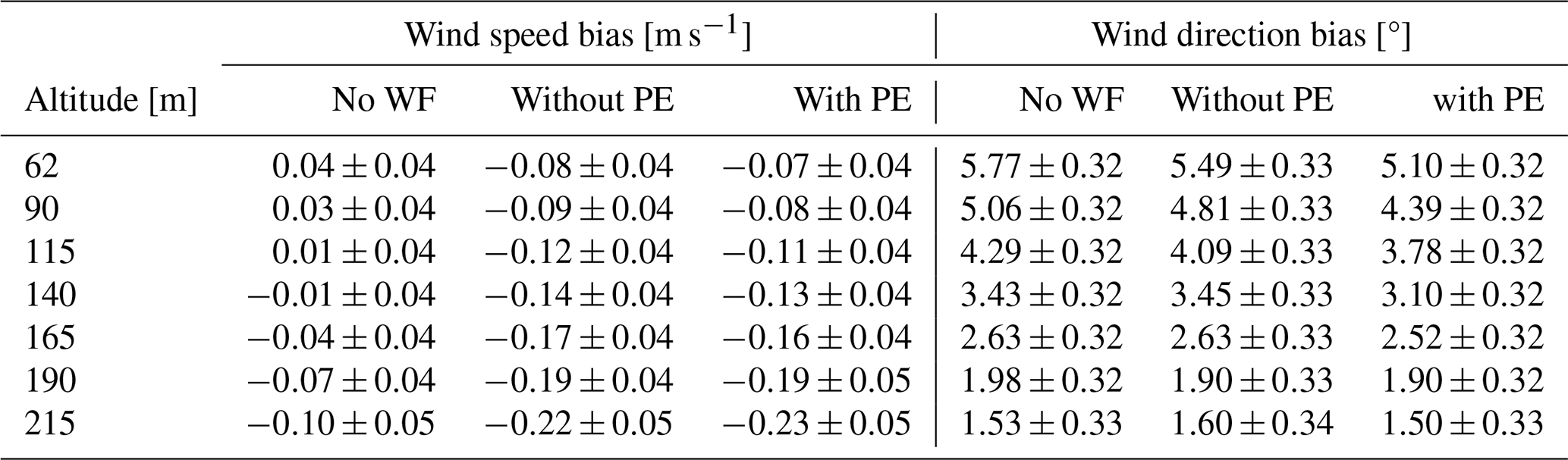
Although optimizing the model setup through an extensive sensitivity study is beyond the scope of this work and has already been addressed elsewhere (Hahmann et al., 2014; Siedersleben et al., 2020; Tomaszewski and Lundquist, 2022; Li et al., 2021; Vermuri et al., 2022), it remains essential to assess the performance of the simulated flow fields relevant to this study. For this purpose, wind speed and wind direction from the no-WF, without-PE, and with-PE simulations are compared against observations at five different locations (Table 1). The mean bias (simulated minus observed) is reported in Tables 4 and 5 for both wind speed and wind direction.

The validation of the ambient wind estimation largely focuses on the no-WF case because the inclusion of wind farms in the simulation causes wakes at the observational mast locations, thus deviating from the observed values, where only a few turbines generated wakes in 2016. This is especially visible at the location of WH, whereas the location in SL is less affected by wakes, as indicated by the smaller differences between the no-WF, without-PE, and with-PE simulations. This is because SL is generally located upstream of the wind farms for the prevailing southwesterly wind direction in this region of the North Sea (Ivanova et al., 2025).

The bias in the simulation without wind farms (no WF) ranges from −0.95 to 0.66 m s⁻¹ for wind speed and −9.85 to 13.71° for wind direction. This falls within the range reported in previous studies on offshore wind fields (Rosencrans et al., 2024; Fischereit et al., 2022b; Borgers et al., 2024; Li et al., 2021). Examining specific observation locations, namely WH, SL, and LG, the wind speed predicted by WRF tends to underestimate observed values offshore, consistent with findings by Li et al. (2021), Rosencrans et al. (2024), and Borgers et al. (2024). In contrast, at WA and SW, closer to the coast, the WRF model tends to overestimate wind speed (Hahmann et al., 2014), suggesting a potential coastal effect not well captured by WRF. Due to the relatively coarse coastal resolution, WRF sees a longer fetch, which results in higher wind speeds in the model (Hahmann et al., 2014). No clear trend is evident in the no-WF biases concerning the altitude of the measurement masts considered, except that the highest observation point exhibits the lowest bias, similar to Klemmer et al. (2024), but opposite to Munoz-Esparza et al. (2012) and Sward et al. (2023).

When comparing all three simulations (no WF, without PE, and with PE), the strongest wake-related biases appear at WH, WA, and SW, where the inclusion of wind farms leads to a significant change in bias compared to the no-WF case. At LG, which is located downwind of the BE–NL wind farm cluster during the prevailing wind direction, some differences between the three simulations can also be linked to wake effects. At WH the differences between the no-WF and without-PE simulations are within the uncertainty range (95 % confidence interval, which accounts for both model variability and, when available, measurement uncertainty; see Appendix C), while the wake effect of the new PE is clearly present in the wind speed bias with PE. At SL, where wakes are not expected to play a large role, the biases are nearly identical across the three simulations. This indicates that the background flow is consistently reproduced in all simulations, providing confidence in the subsequent wake energy loss analysis.

The lidar at LG was designed specifically for assessing offshore wind resources. It provides vertical wind profiles up to 215 m, enabling model evaluation at heights comparable to the level of turbine hub heights. Comparing the different WRF simulations with the lidar observations (Table 5) reveals a small mean bias across all altitudes and different simulations. The bias for wind speed ranges from 0.04 m s⁻¹ at 62 m to −0.10 m s⁻¹ at 215 m in the no-WF simulation, from −0.08 m s⁻¹ at 62 m to −0.22 m s⁻¹ at 215 m in the without-PE simulation, and from −0.07 m s⁻¹ at 62 m to −0.23 m s⁻¹ at 215 m in the with-PE simulation, respectively. Wind direction biases gradually decrease with height, ranging from values around 5° at 62 m to around 1.5° at 215 m. This suggests improved directional agreement at higher altitudes. The mean wind speed and direction bias of different simulations often fall within the observational uncertainty, accounting for model variability and lidar measurement error, especially between the without-PE simulation and the with-PE simulation. Larger differences are observed when comparing to the no-WF simulation; this could be caused by wakes. To conclude, the background wind field can be assumed to be similar across simulations, justifying studying the wake effects in the suggested simulations. Overall, based on all observation comparisons, a good agreement between modeled and observed values at hub height supports using WRF to evaluate wake impacts of the newly built PE on existing wind farms.

Table 4 Mean wind speed [m s⁻¹] and wind direction [°] bias (simulation − observations) and the 95 % confidence interval, which accounts for both model variability and, when available, measurement uncertainty, for the no-WF WRF as well as the without-PE and with-PE simulations at the five different observation locations (Table 1).

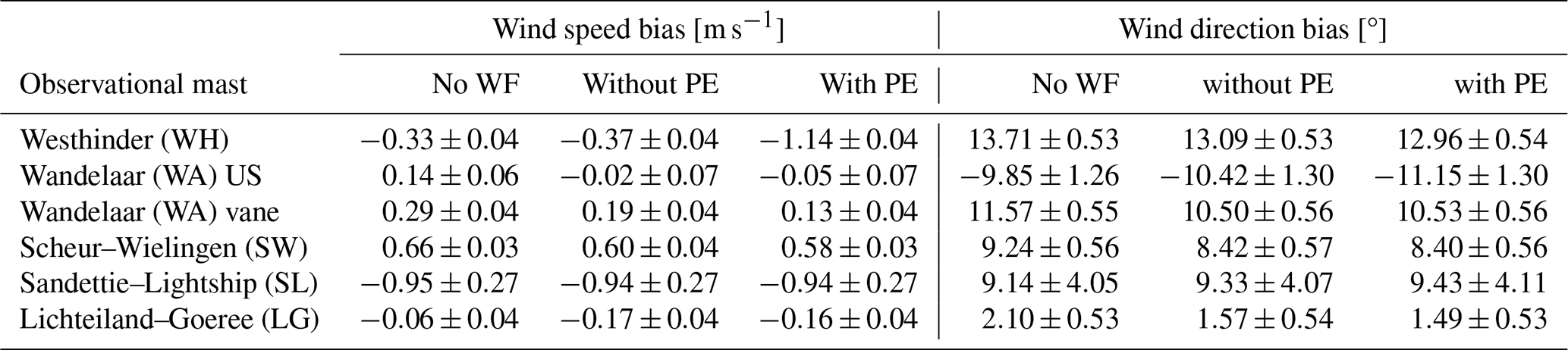
Table 5 Mean wind speed [m s⁻¹] and wind direction [°] bias (simulation - observations) and the 95 % confidence interval, which accounts for both model variability and, when available, measurement uncertainty, for the no-WF WRF as well as the without-PE and with-PE simulations at different altitudes of the LG lidar location (Table 1).

3.2 AEP losses compared to spatiotemporally averaged internal and external wake energy losses

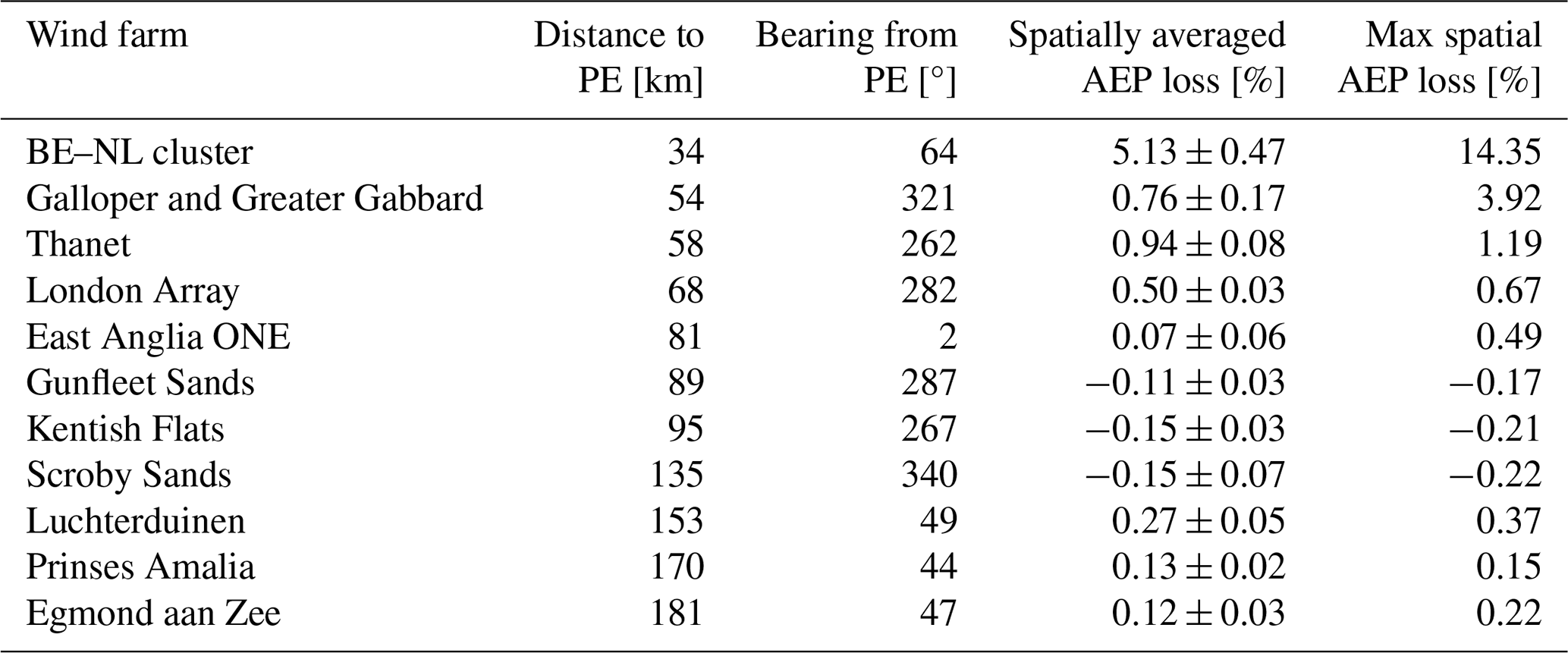
The annual energy production (AEP) and mean yearly wind speed deficit before (Fig. 3a, b) and after constructing the new Princess Elisabeth wind farm cluster (Fig. 3c, d) are shown. The wind speed deficit at the mean hub height (96 m) of the wind farms is defined as the temporally averaged wind speed of the simulation, which could be with PE or without PE, minus the temporally averaged wind speed of the no-WF simulations. Figure 3e and f show the effect of constructing the new Princess Elisabeth wind farm cluster. The wind farm cluster most affected by the new PE wind farm cluster is the Belgian–Dutch (BE–NL) wind farm cluster (Fig. 1), with differences in annual energy production (AEP) up to 14 % at certain grid cell locations and 5 % spatiotemporally averaged over the wind farm cluster (Table 6). This effect is primarily due to the proximity of this cluster to the Princess Elisabeth wind farm and its downstream location for the main wind direction, which is southwesterly (Ivanova et al., 2025). The BE–NL cluster experiences the most significant impact, but smaller effects are also observed for wind farms further away. Table 6 shows that distance alone does not explain the magnitude of the AEP impact, highlighting the importance of the relative location of the wind farm with respect to the prevailing southwesterly winds. For instance, a wind farm located at a distance of 181 km exhibits a small AEP loss of 0.12 %. While the 95 % confidence interval of the simulated AEP difference excludes zero, indicating a statistically significant difference, such a small value is unlikely to represent a physical wake impact and is more probably explained by numerical variability in the WRF simulations. It is important that further research investigates these small wake impacts and assesses whether such small values hold physical or economic significance. The observed long-distance impacts underscore the importance of accounting for AEP losses in both existing and planned wind farms during future siting decisions and yield assessments. This applies not only to nearby wind farms, but also to more distant farms. This consideration becomes increasingly important as the density of offshore wind farms is projected to increase in the coming years (Borgers et al., 2024). It should also be noted that very small increases (0.11 %–0.15 %) in AEP are seen for three wind farms after the construction of the PE wind farm. Given the low magnitude and the fact that these occur at only three locations, it is difficult to draw any strict conclusions regarding actual increases in AEP. These increases in AEP may be attributable to numerical variability, possibly related to coastal effects or model variability in WRF, and further research would be needed to determine whether they have physical (flow speedup) or economic significance.

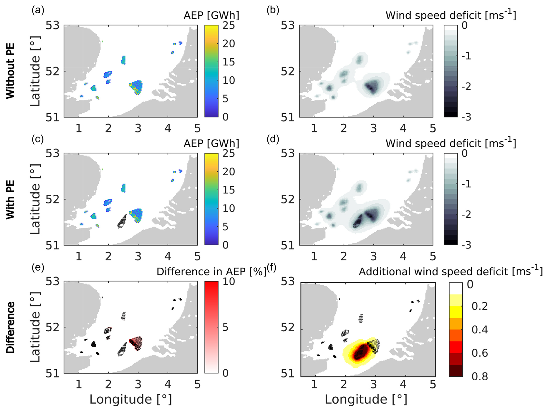
Figure 3 Annual energy production (a, c, e) and temporally averaged wind speed deficit (b, d, f) before (a, b) and after (c, d) the construction of the PE wind farm cluster. The bottom row shows the difference between the two top rows (e, f).

Due to the presence of the new PE wind farm cluster, wind deficits are intensified (maximum deficit increasing from 2.7 to 2.9 m s⁻¹) and spread over a larger region (Fig. 3b, d, f). This effect is attributed to the increased momentum extraction of the 15 MW turbines of the PE wind farm cluster. The wind speed deficit exerts the strongest influence in the wake of the main wind direction, which is southwesterly (Ivanova et al., 2025). However, wind speed deficits are also observed southwest of the PE farms and extend toward the northwest of the future concession. These wind speed deficits contribute to changes in AEP, although the relationship between wind speed reduction and power loss is not proportional, as power production depends nonlinearly on wind speed. This nonlinearity has also been highlighted in recent studies on cluster wake-induced energy losses (Xia et al., 2025). Consequently, regions experiencing the strongest wind speed deficits generally correspond to areas of larger AEP losses, but even small changes in wind speed may produce disproportionately larger or smaller impacts on AEP depending on the turbine operating regime. It is also important to note that the wind speed deficits mentioned here are temporally averaged (annual) deficits, and their strength and direction are strongly dependent on wind direction and stability, as discussed in the following sections. Previous work showed that it is less dependent on the TKE coefficient (Rosencrans et al., 2024).

Table 6 Distance to the PE wind farm cluster (center to center), direction from the PE wind farm cluster to the wind farm centroid, spatially averaged AEP loss over each wind farm (with ±95 % confidence interval from 1000 bootstrap resamples), and the spatial maximum AEP loss within each farm.

As shown in Table 7, the internal wake energy losses (i.e., wake losses experienced by the existing wind farms in the absence of the PE wind farm cluster) are larger than the external wake energy losses (i.e., the additional wake losses induced by the PE wind farm cluster). Note that internal wake energy losses do not refer to the strict definition of internal wake losses but to the energy losses caused in the absence of the PE wind farm cluster (Sect. 2.5). For all the simulated wind farms, the internal wake energy losses are greater than 20.99 %, and they reach as high as 42.01 % for the BE–NL wind farm cluster. These losses are spatiotemporally averaged wake energy losses. WRF simulations of planned wind farm deployments along the east coast of the United States also predict internal wake losses of a similar magnitude, despite differences in wind farm configuration (Rosencrans et al., 2024; Rybchuk et al., 2022). It is known that the WRF model with the wind farm parameterization of Fitch (Fitch et al., 2012) can overestimate internal wake power losses because turbine wakes are distributed over grid cells much larger than individual wakes, and turbulence generation is also underrepresented (Abkar and Porté-Agel, 2015; Sanchez Gomez et al., 2024). As such, the results shown in Table 7 may be an upper estimate of internal wake energy losses. Future comparisons with operational SCADA could assess this in more detail.

Relative to the internal wake losses, the external wake losses are generally much smaller (Table 7). For several distant wind farms, such as Scroby Sands, East Anglia ONE, Kentish Flats, Egmond aan Zee, Gunfleet Sands, and Prinses Amalia, the 95 % confidence intervals of the external wake losses include zero. This suggests that the estimated external wake losses for these distant farms are not statistically distinguishable from zero and may reflect numerical variability or random fluctuations rather than a true physical wake effect. In contrast, only closely located farms such as the BE–NL cluster, Galloper and Greater Gabbard, London Array, Thanet, and Luchterduinen show statistically significant external wake losses.

Table 7 Spatiotemporally averaged external and internal wake energy losses over different wind farms. Uncertainty is reported as the half-width of the 95 % confidence interval from 1000 bootstrap resamples.

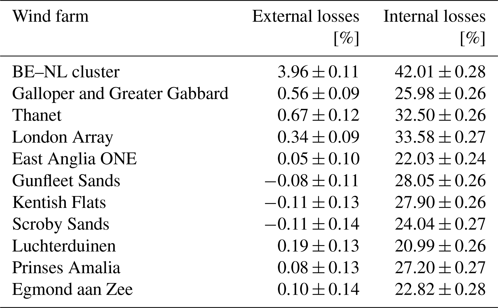
Comparing the external wake energy losses (Table 7) with the AEP losses (Table 6) shows that both tables exhibit similar spatial trends. The BE–NL wind farm cluster, Galloper and Greater Gabbard, London Array, Thanet, and Luchterduinen show the largest impacts, while more distant farms show much smaller effects. Differences between the two tables arise because the metrics are defined using different normalizations. The AEP losses are computed as relative changes between the without-PE and with-PE simulations and normalized by AEP without PE, whereas the external wake losses are defined as ratios of temporally averaged power normalized by the no-WF simulation (Eqs. 4–6). This difference in normalization, together with the implicit weighting of high-production periods in the AEP calculation, explains why some farms show statistically significant AEP impacts, while their external wake losses are not statistically significant.

3.3 External wake energy losses as a function of wind direction, wind speed, and atmospheric stability

To gain more insight into the atmospheric conditions influencing external wake energy losses (defined in Sect. 2.5) a more in-depth study of the BE–NL wind farm cluster (Fig. 1 – K) is conducted. This wind farm cluster is investigated because it experiences the largest wake losses. In all following figures we characterize the atmospheric conditions (wind direction, atmospheric stability class, and wind speed) based on a reference location (spatially averaged grid cell location of the considered BE–NL wind farm cluster) of the no-WF WRF simulation. The height at which the wind speed and direction are taken is 96 m altitude, which is the weighted averaged hub height over all wind turbines considered in this work. The error bars in the following figures represent a 95 % confidence interval calculated by bootstrapping with 1000 resamples.

In Fig. 4a, we show the annually averaged external wake energy losses of the BE–NL wind farm cluster caused by the PE wind farm cluster. We also show how this external wake energy effect depends on wind direction (Fig. 4b), stability (Fig. 4c), and wind speed (Fig. 4d). We note that each of these figures (Fig. 4b–d) only looks at a single variable in isolation and does not control for the other variables simultaneously, which can be important due to the inherent correlations between wind direction, wind speed, and stability. This means that the patterns in Fig. 4b–d reflect combined effects rather than the influence of a single variable. Temperature inversion height may also contribute to the observed stability dependence of wake losses and could be investigated in future work.

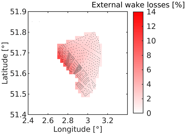
The external wake energy losses are spatially concentrated at the top left corner of the BE–NL wind farm cluster, resulting in external energy wake losses up to 10 % at these grid cell locations (Fig. 4a). These high losses are linked to the prevailing southwesterly wind direction of approximately 225°, leading to the highest losses in this part of the cluster, as the new PE wind farm is upstream of the BE–NL cluster for this wind direction (Figs. 4b and 5). For wind directions outside the range where BE–NL is directly in the wake of PE, the new PE wind farm cluster induces small external wake energy losses (Fig. 4b). In some directions, negative wake energy losses are observed, which imply a limited power gain after the PE wind farm cluster was constructed. This is discussed later in the paper.

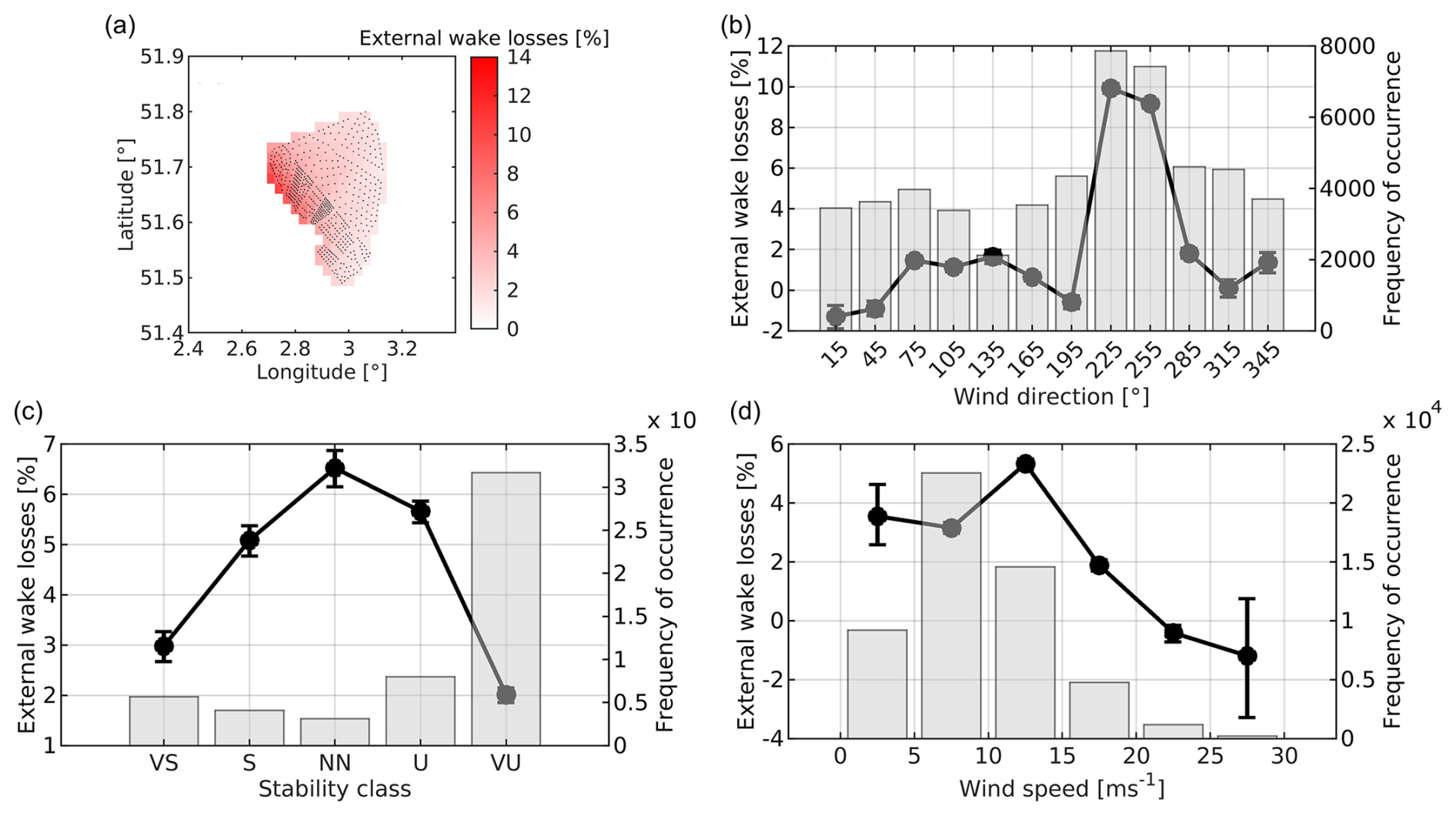
Figure 4 Results are shown for the BE–NL wind farm cluster. (a) Temporal average of external wake energy losses for the BE–NL wind farm. (b) Line: spatiotemporal conditional average of external wake energy losses as a function of wind direction; bars: frequency of occurrence of the different wind directions. (c) Line: spatiotemporal conditional average of external wake energy losses as a function of atmospheric stability class (VS: very stable; S: stable; NN: near neutral; U: unstable; VU: very unstable); bars: frequency of occurrence for the different atmospheric stability classes. (d) Line: spatiotemporal conditional average of external wake energy losses as a function of wind speed; bars: frequency of occurrence of the different wind speeds. The error bars represent a 95 % confidence interval obtained via bootstrapping with 1000 resamples.

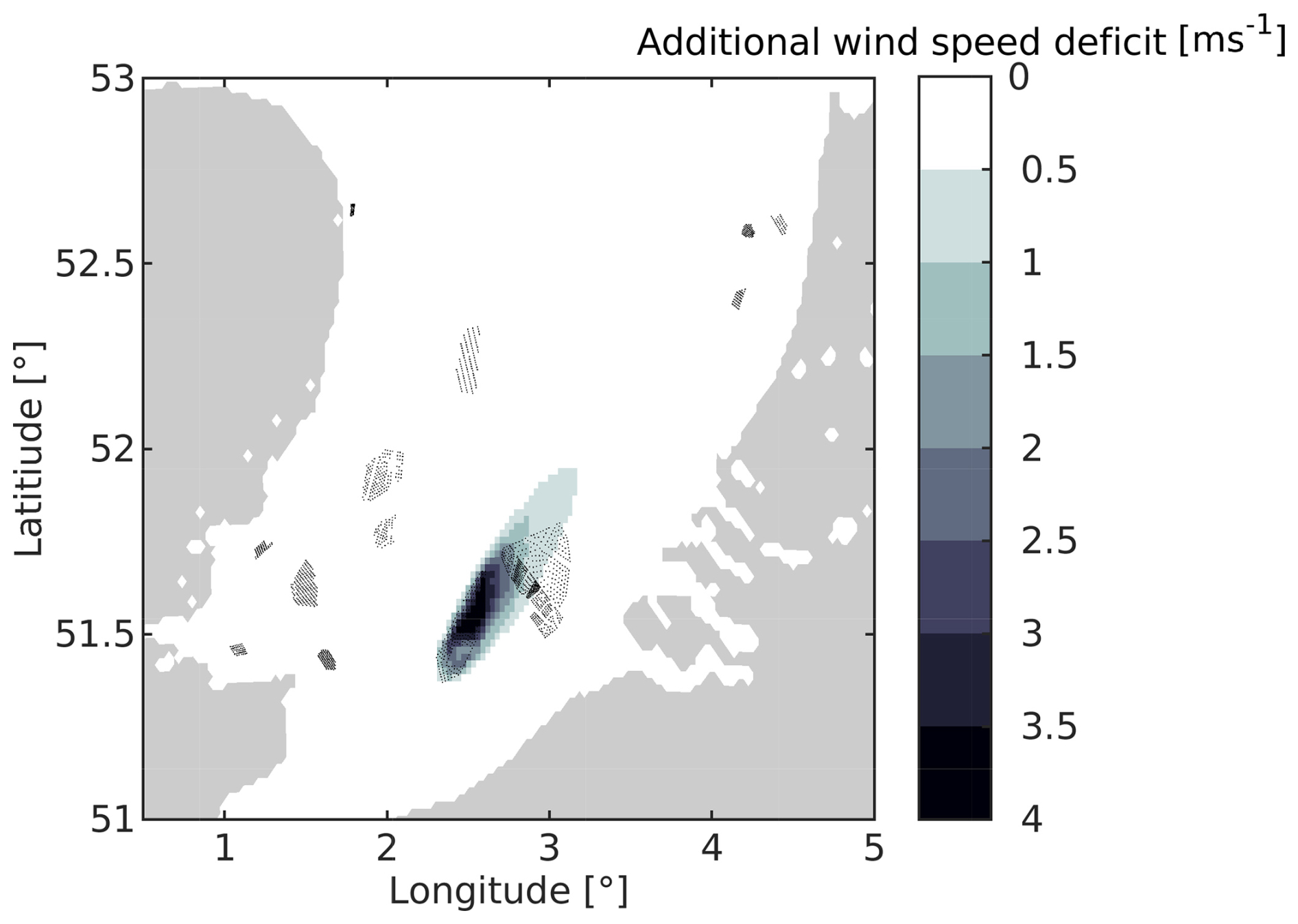
Figure 5 External BE–NL wind farm wake deficit for wind directions between 215 and 235°, which corresponds to the highest external wake losses and the most frequent wind direction.

Figure 4c shows the external wake energy losses as a function of atmospheric stability. In this figure, the highest losses are present for near-neutral conditions. This arises because the figure does not control for wind conditions, and aggregating over all atmospheric situations allows competing effects to cancel or amplify, which obscures the underlying stability dependence. To elucidate how the wake effects depend on stability more clearly, we define a restricted wind direction bin of 193 to 317°. This wind direction bin only includes wind directions for which the BE–NL wind farm cluster is in the wake of the PE wind farm cluster. These results are shown in Fig. 6 and show generally decreasing external wake energy losses from a very stable to a very unstable atmosphere. The lowest external wake energy losses are present for the most frequently occurring very unstable atmospheric conditions. It has been reported in earlier studies that, for the North Sea, (very) unstable atmospheric conditions are commonly seen (Porchetta et al., 2019; Munoz-Esparza et al., 2012; Nybø et al., 2020). Stable conditions in the North Sea (BE–NL wind farm cluster) are often associated with southwesterly wind directions, when warmer air is transported over the colder sea, particularly during spring and summer. However, this pattern is site-dependent, as stability is strongly influenced by the temperature contrast with the nearest coastline. For other wind directions, particularly those bringing colder air over a relatively warmer sea, especially in winter, (very) unstable conditions tend to dominate (Nybø et al., 2020; Cheynet et al., 2018).

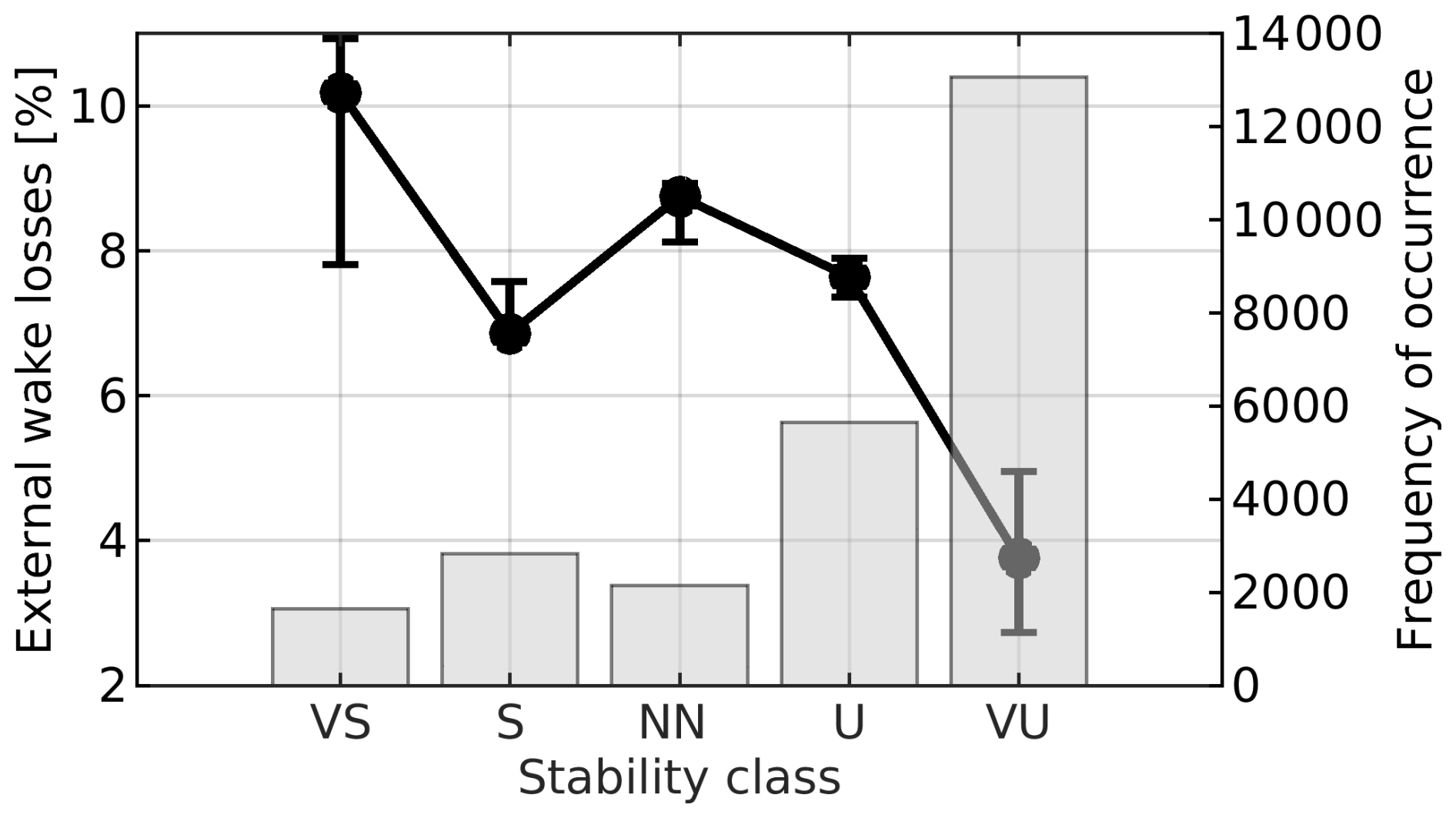
Figure 6 Line: spatiotemporal conditional average of external wake energy losses as a function of atmospheric stability class (VS: very stable; S: stable; NN: near neutral; U: unstable; VU: very unstable) only including wind directions from 193–317°; bars: frequency of occurrence for the different atmospheric stability classes. The error bars represent a 95 % confidence interval obtained via bootstrapping with 1000 resamples.

External wake energy losses are expressed as percentages (Eq. 6). At lower wind speeds, turbines produce little power, so even small external wake energy losses appear as relatively large percentage losses (Fig. 4d), even though the absolute wake effect may not be stronger. At the same time, turbine thrust coefficients are higher at low wind speeds, potentially leading to longer wake recovery distances. In contrast, when examining absolute losses (Fig. 7), the largest deficits occur for wind speeds between 10 and 15 m s⁻¹ (mostly Region II). In this range, turbines operate close to rated power while still generating high thrust, so wakes cause large power losses. At higher wind speeds, the thrust coefficients decrease, and turbines typically remain at rated power even in the presence of wakes.

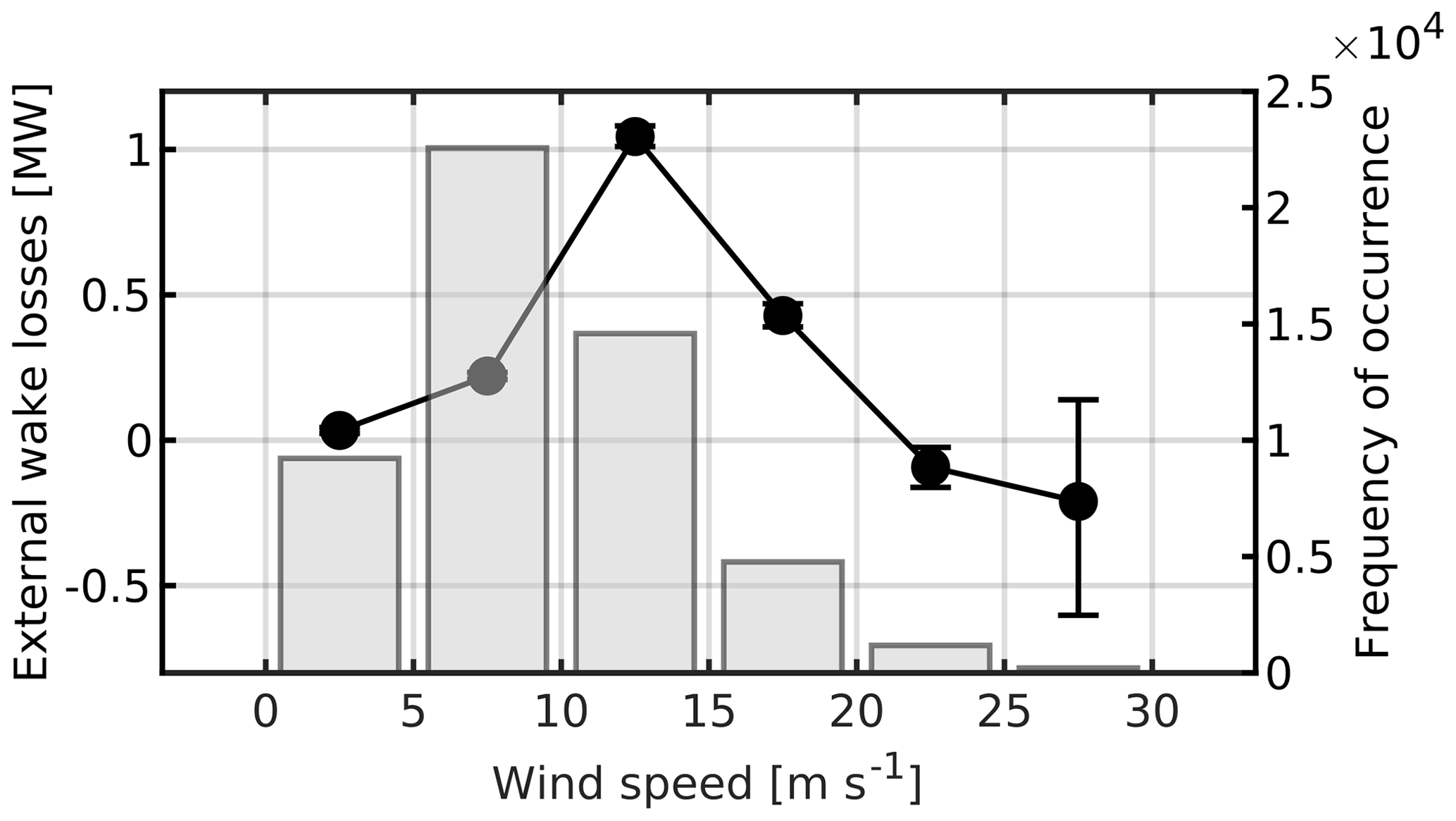
Figure 7 Line: spatiotemporal conditional average of absolute external wake energy losses as a function of wind speed; bars: frequency of occurrence for the different wind speed bins. The error bars represent a 95 % confidence interval obtained via bootstrapping with 1000 resamples.

Interestingly, negative external wake energy losses (−1 %), i.e., positive interference from the construction of the new PE wind farm cluster, are observed for winds coming from the north to northeast (0–60°) or south (180–210°) (Fig. 4b). The negative external wake energy losses for wind directions from the south can be explained by a speedup at the lateral locations of the PE wind farm clusters (Fig. 8). It appears that the PE wind farm cluster acts as a windbreak, causing global blockage and accelerating the flow around sides of the wind farm (Porté-Agel et al., 2020). A comparable lateral acceleration caused by global blockage is reported for certain North Sea wind farm clusters (Borgers et al., 2025). While similar effects have been studied for windbreaks, where they mainly cause vertical speedups (Liu and Stevens, 2021), lateral flow accelerations influencing farm-to-farm wakes have received comparatively limited attention in the literature (Hasager et al., 2015; Nygaard and Hansen, 2016; Borgers et al., 2025). Nygaard and Hansen (2016) observed this farm effect based on measured wind turbine data from two offshore wind farms. This speedup effect in the lateral direction has been observed multiple times for individual wind turbines (Ammara et al., 2002; Araya et al., 2014; Puccioni et al., 2023). In the coming years, it would be beneficial to enhance our understanding of this acceleration phenomenon around wind farms through idealized simulations; however, this is outside the scope of this work. Understanding these speedups is important, as they may have a significant impact on external wake energy losses, necessitating consideration in the planning of high-density offshore regions.

Why negative external wake energy losses are observed for wind directions from the north to northeast is less clear. As mentioned previously for the AEP losses, these may result from numerical variability or other uncertainties in the simulation. The underlying mechanisms of these minor effects, which might be physical or not, should be investigated in the future.

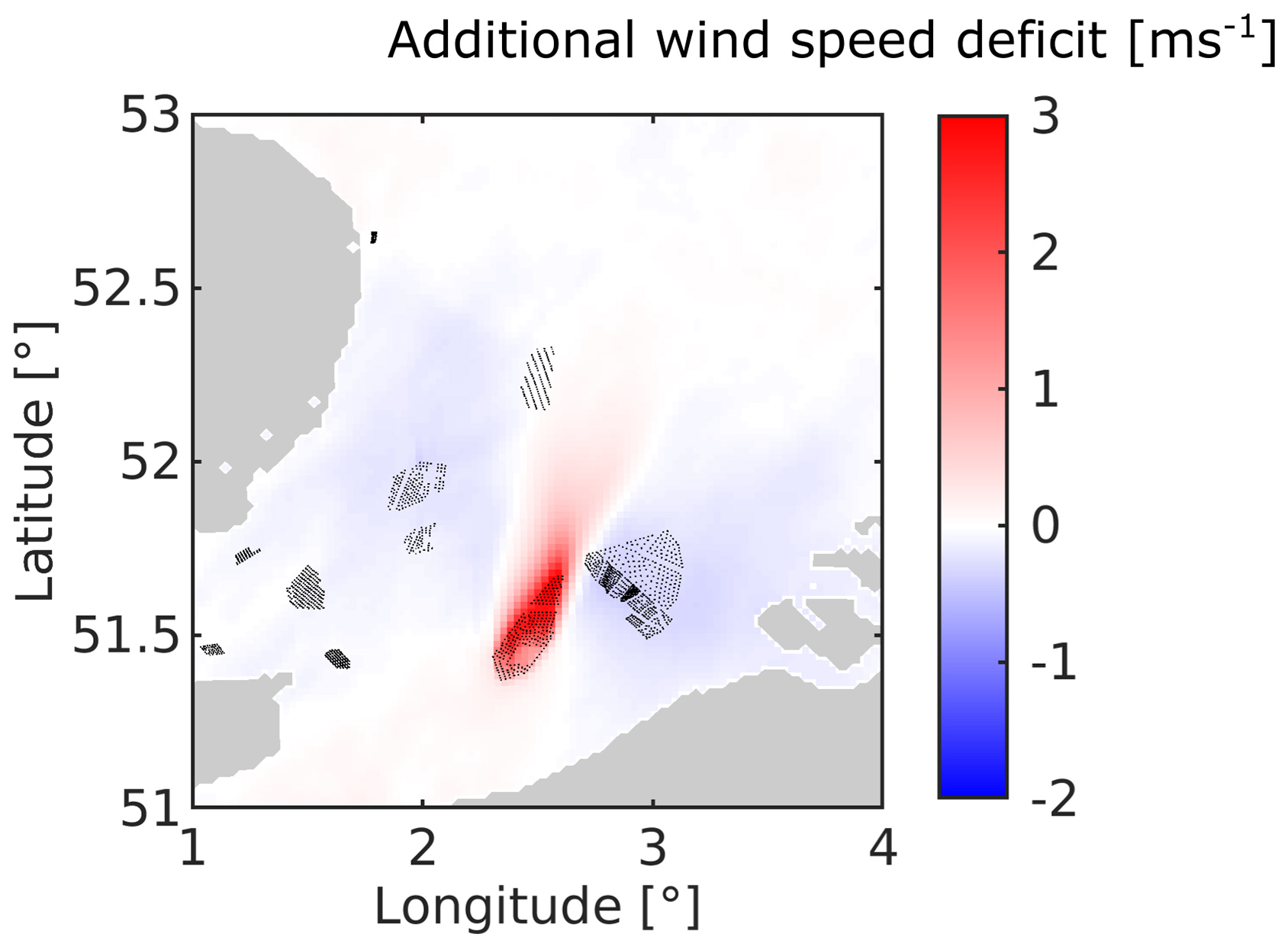
Figure 8 This map shows the additional wind speed deficit for wind directions between 180 and 210° after the construction of the PE wind farm for time steps with negative external wake energy losses over the farm.

3.4 Internal wake energy losses as a function of wind direction, wind speed, and atmospheric stability

The yearly averaged internal wake energy losses are shown in Fig. 9a. At specific locations within the BE–NL wind farm cluster (grid level), the internal wake energy losses reach as high as 53 %, which are similar to values in previous studies (Rosencrans et al., 2024; Rybchuk et al., 2022). These high internal wake energy losses are associated with very dense wind farm layouts. As mentioned previously, WRF with the Fitch wind farm parameterization is known to overestimate the internal wake losses (Sanchez Gomez et al., 2024; Abkar and Porté-Agel, 2015), and the results here thus show the upper limit.

Figure 9b shows the spatiotemporal internal wake energy losses as a function of wind direction. The high internal wake energy losses are associated with wind directions for which many turbines are aligned in the flow direction. Unlike the external wake energy losses (Fig. 4b), which are dominated by wind directions for which the wind farms are waked by the PE wind farm cluster, the internal wake energy losses are strongest for the least frequent southeasterly wind direction (occurring only 4 % of the time). This wind direction corresponds to conditions under which the largest number of turbines are influenced by upstream turbines within the same wind farm cluster.

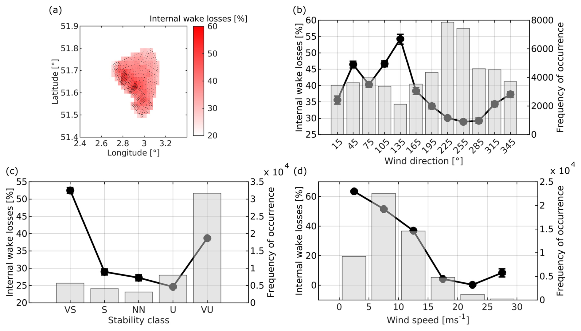
Figure 9 Results are shown for the BE–NL wind farm cluster. (a) Temporal average of internal wake energy losses for the BE–NL wind farm. (b) Line: spatiotemporal conditional average of internal wake energy losses as a function of wind direction; bars: frequency of occurrence of the different wind directions. (c) Line: spatiotemporal conditional average of internal wake energy losses as a function of atmospheric stability class (VS: very stable; S: stable; NN: near neutral; U: unstable; VU: very unstable); bars: frequency of occurrence for the different atmospheric stability classes. (d) Line: spatiotemporal conditional average of internal wake energy losses as a function of wind speed; bars: frequency of occurrence of the different wind speeds. The error bars represent a 95 % confidence interval obtained via bootstrapping with 1000 resamples.

Figure 9c shows the internal wake energy losses as a function of atmospheric stability. The internal wake energy losses generally decrease from stable to unstable conditions, with an apparent increase for very unstable conditions. Similar to the external wake energy losses, this may seem counterintuitive, but it arises because this figure does not control for wind speed or wind direction and instead aggregates all atmospheric conditions. After additionally conditioning on wind speeds between 10 and 15 m s⁻¹, a clear pattern of decreasing internal wake energy losses with increasing atmospheric instability emerges (Fig. 10), as expected. Since very unstable conditions occur most frequently, a large number of low-wind-speed events are included, which increases the relative percentage losses and therefore results in higher apparent internal wake energy losses. This is consistent with the findings of Xia et al. (2025), who showed that wind speed deficits do not translate linearly into power or energy losses.

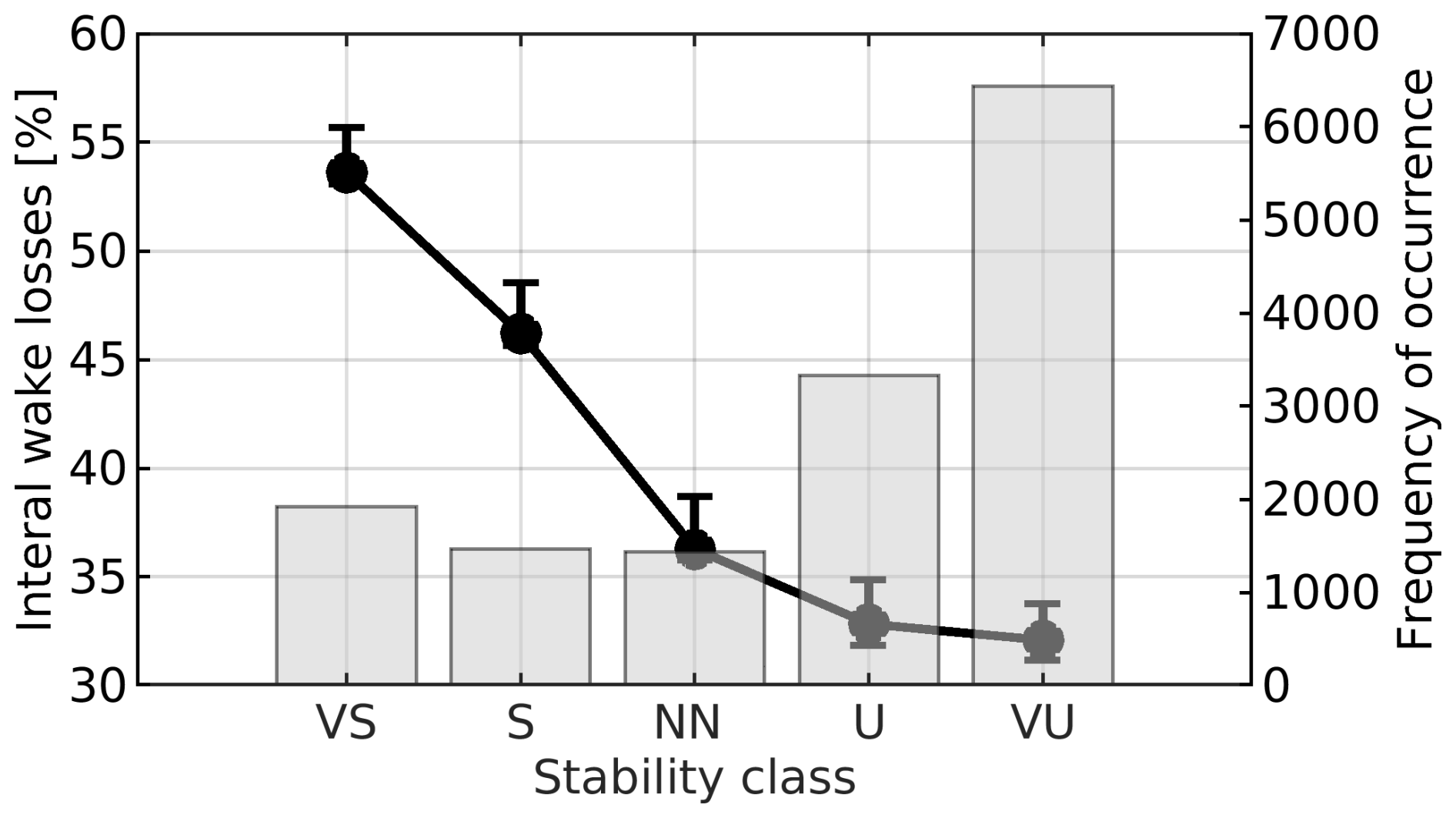
Figure 10 Line: spatiotemporal conditional average of internal wake energy losses as a function of atmospheric stability class (VS: very stable; S: stable; NN: near neutral; U: unstable; VU: very unstable) only including wind speeds between 10 and 15 m s⁻¹; bars: frequency of occurrence for the different atmospheric stability classes. The error bars represent a 95 % confidence interval obtained via bootstrapping with 1000 resamples.

For the internal wake energy losses as a function of velocity we observe the same behavior as for the external wake losses. When expressed as percentages, they are larger at lower wind speeds because the denominator is small, so even modest absolute deficits translate into large relative losses (Fig. 9d). In contrast, when considering absolute losses, the largest deficits occur between 10 and 15 m s⁻¹, when turbines operate close to rated power with high thrust coefficients, and wakes cause substantial power losses (Fig. 11). At higher wind speeds, turbines remain at rated power, which limits the relative impact of internal wake losses.

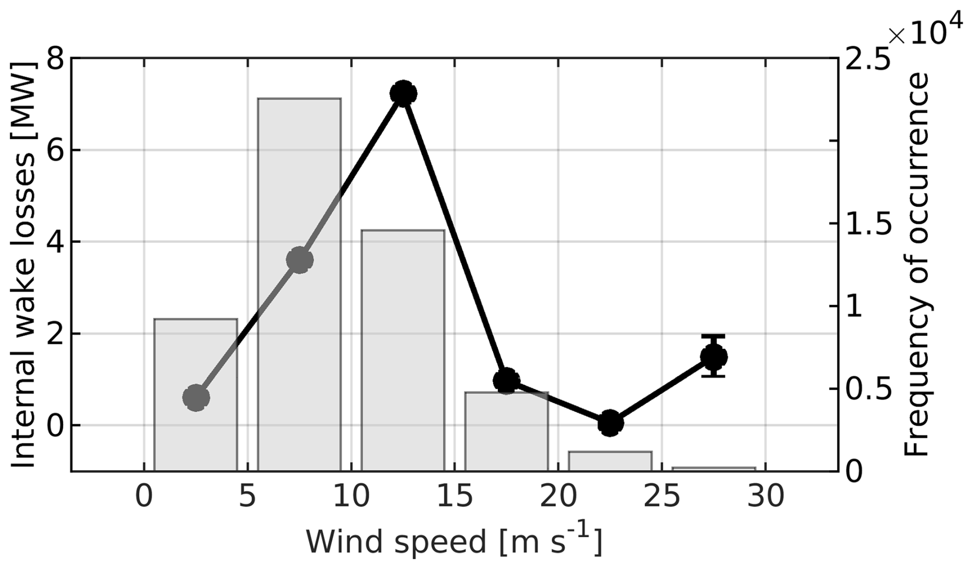
Figure 11 Line: spatiotemporal conditional average of absolute internal wake energy losses as a function of wind speed; bars: frequency of occurrence for the different wind speed bins. The error bars represent a 95 % confidence interval obtained via bootstrapping with 1000 resamples.

3.5 Internal wake evolution across successive turbine-containing grid cells

To better understand the interaction between external and internal wake effects, we investigate how the presence of wakes from the upstream PE wind farm cluster modifies the development of internal wakes within the downstream BE–NL wind farm cluster. To this end, we analyze five successive turbine-containing grid cells for two representative wind directions, one for which the BE–NL cluster is not affected by PE wakes and one for which it is. In Fig. 12, we demonstrate that the structure of the internal wake of the selected wind turbines is affected by the new upstream PE wind farm cluster. If the turbines are not in the wake of the upstream PE wind farm cluster the internal wake is unaffected by the presence of the new PE wind farm cluster (Fig. 12a–e). However, the internal wakes of the selected wind turbines of the downwind farm that are in the wake of the new PE wind farm cluster undergo nonlinear effects (Fig. 12f–j). The power normalized by the first-row turbines is higher for the turbines when they are waked by the PE wind farm cluster (Fig. 12h). This increase in power could be caused by a higher added TKE compared to the simulation without the new PE wind farm cluster (Fig. 12j), which enhances the mixing of the wake and thus dissipates the wake faster. Additionally, the velocity deficit is smaller for the waked turbines, which additionally results in higher power after the front-row wind turbine (Fig. 12i). Together, the new PE wind farm cluster lowers the overall power of the turbines (Fig. 12g), but it also reduces the internal wake energy losses (Fig. 12h). These phenomena again emphasized the caution that should be paid in the future for farm–farm interactions, as they can induce nonlinear effects within a distant wind farm.

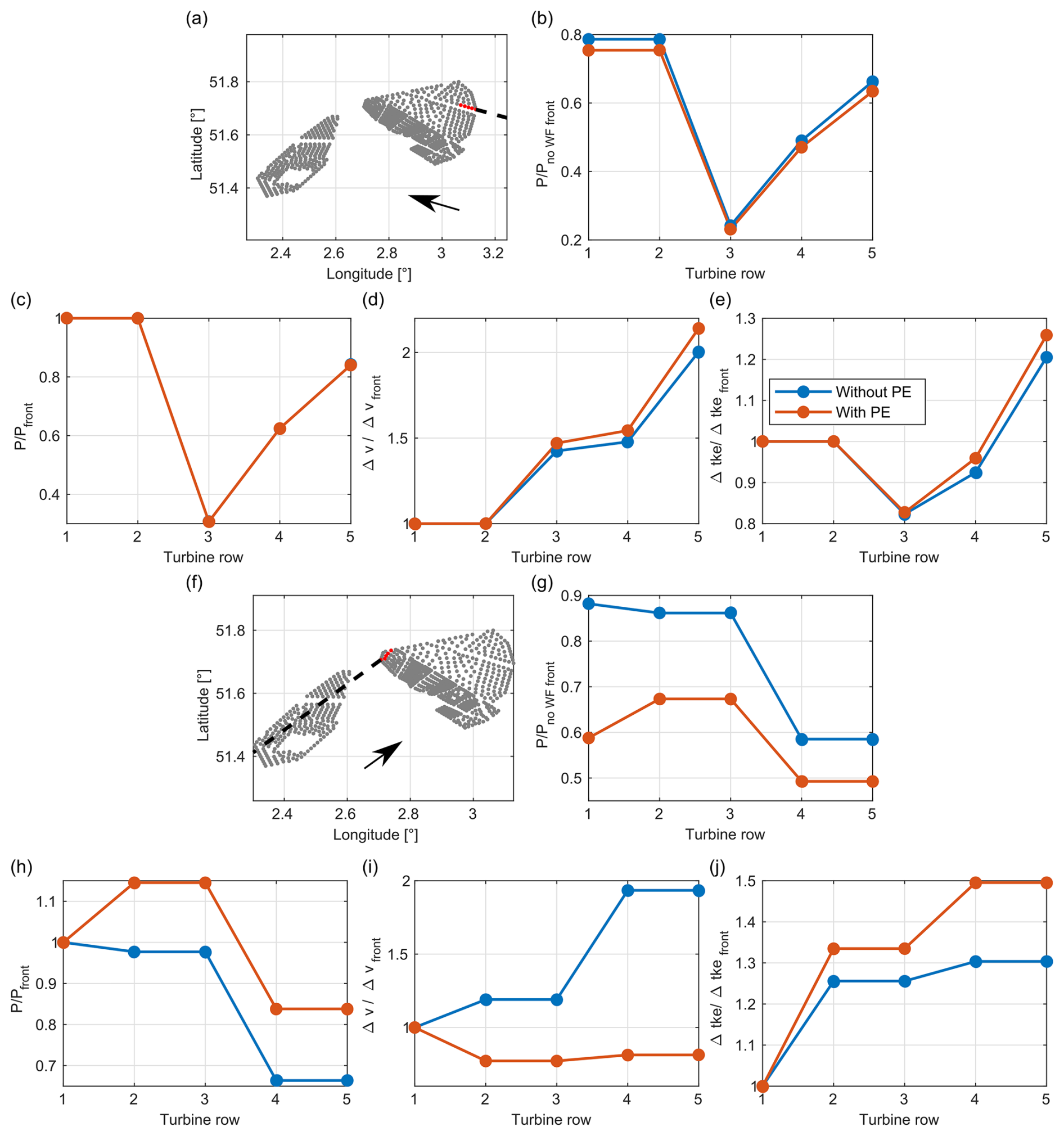
Figure 12 (a, f) Wind turbine locations considered for two representative wind directions (black arrows): (a) 105°, corresponding to a case where the BE–NL wind farm cluster is not influenced by wakes from the PE wind farm cluster, and (f) 234°, corresponding to a case where the BE–NL cluster is waked by the PE wind farm cluster. The red dots indicate the turbine used for the analysis. Panels (b)–(e) and (g)–(j) show turbine quantities as a function of turbine row number, illustrating how wake interactions evolve through the wind farm under unwaked and waked conditions (blue and orange, respectively). Specifically, (b) and (g) show turbine power normalized by the no-WF front-row turbine power, (c) and (h) show turbine power normalized by the front-row turbine power, (d) and (i) show wind speed deficits relative to the no-WF simulation and normalized by the front row, and (e) and (j) show added TKE relative to the no-WF simulation and normalized by the front row.

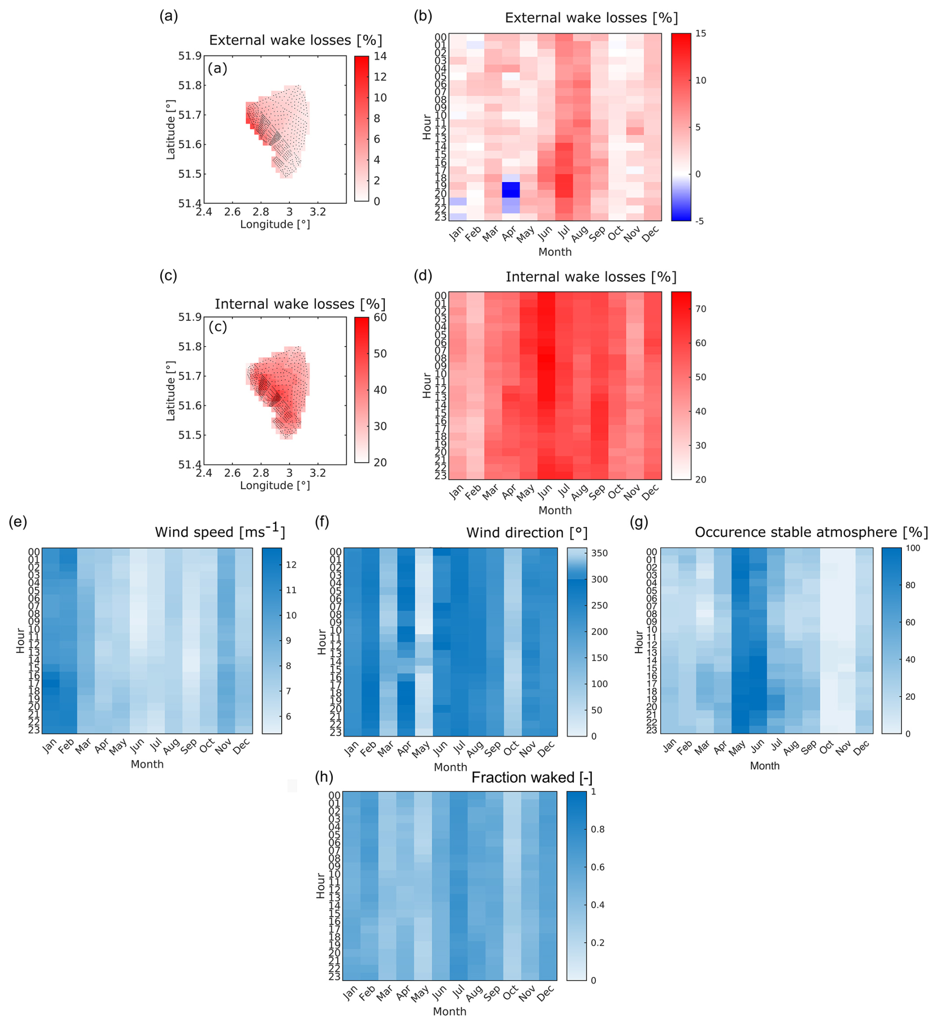
Figure 13 Results are shown for the BE–NL wind farm cluster. (a) Temporal-average external wake energy losses. (b) Hourly and monthly variations in the spatiotemporally averaged external wake energy losses. (c) Yearly averaged internal wake energy losses. (d) Hourly and monthly variations in the spatiotemporally averaged internal wake energy losses. Hourly and monthly variations in (e) wind speed, (f) wind direction, (g) occurrence of stable atmospheric conditions, and (h) fraction of wind directions within the PE wind farm cluster wake (193–317°), with 1 corresponding to waked and 0 to non-waked conditions. Hourly variations are given in UTC.

3.6 Hourly and monthly variation in external and internal wake energy losses

Due to the temporal variability in atmospheric conditions, the yearly averaged wake energy losses are not informative about which atmospheric conditions are more critical to induce larger internal or external wake energy losses. As mentioned earlier the atmospheric conditions (wind direction, atmospheric stability class, and wind speed) are based on a reference location (spatially averaged grid cell location of the considered BE–NL wind farm cluster) of the no-WF WRF simulation at a height of 96 m. There is a different behavior, at both hourly and monthly timescales, between the external and internal wake energy losses (Fig. 13b and d). The hourly variation is stronger for external wake energy losses compared to internal wake energy losses, and both vary seasonally. Larger external wake energy losses are observed in summer during the late afternoon, while the internal wake energy losses' variability is mainly determined by the season. The higher external wake energy losses in summer are explained by the lower wind speeds that coincide with the steep ramp of the power curve and have higher turbine thrust coefficients (Fig. 13e) and the higher occurrence of stable atmospheric conditions (Fig. 13g), when warm air is advected over the colder water (Rosencrans et al., 2024). Additionally, these higher external wake losses coincide with increased fraction of time during which the wind farm is waked by the upstream PE wind farm cluster (Fig. 13h). In contrast, lower wake energy losses in winter occur for higher wind speed and more unstable atmospheric conditions (Fig. 13e and g), when cold air moves across the warmer water (Rosencrans et al., 2024). It should be noted that these results are based on 1 year of data, and therefore any generalization of the diurnal and seasonal variation should be made with caution. In addition, further investigation to better understand the occurrence of negative external wake losses during the evening hours in spring is required in the future but is outside the scope of this paper.

4 Conclusions

The yearly averaged and the sub-annual variation in the wake energy losses of a new wind farm cluster on adjacent, existing wind farms is studied for the new Princess Elisabeth wind farm cluster. The wake impacts of a representative year have been simulated with the mesoscale model WRF to estimate representative wake energy losses.

The mesoscale model predicts that building the new Princess Elisabeth wind farm cluster gives differences up to 5 % of AEP for a closely located neighboring wind farm. The external wake energy losses of this closely located neighboring wind farm are mainly determined by the waked wind direction of the Princess Elisabeth wind farm cluster, stable conditions, and Region II wind speeds. The largest internal wake energy losses occur for wind directions for which many turbines within the wind farm are aligned with the incoming flow. Additionally, the interaction with the new wind farm cluster induces a nonlinear modification of the internal wake dynamics, whereby increased turbulence promotes wake recovery and partially offsets internal wake losses within the downwind farm. Interestingly, some wind farms located farther away show negative wake losses. For closely located farms, such negative values can in part be explained by specific wind directions where a lateral speedup occurs at the flanks of the upstream wind farm. However, for more distant farms, negative wake losses but also very small positive values could be due to numerical variability or other simulation uncertainties. A more in-depth study of these values and their significance is needed in future work.

These internal and external wake energy losses are investigated by hour and month. The external wake energy losses exhibit a stronger hourly variation, while the internal wake energy losses depend strongly on season. These temporal variations can largely be explained by differences in atmospheric stability and wind speed, with stable conditions and below-rated wind speeds resulting in higher wake energy losses (Porchetta et al., 2026).

This study provides a year-long WRF data set that quantifies the magnitude of external and internal wake effects expected under future North Sea wind power development. We also show how these wake effects depend on season, hour of the day, wind speed, wind direction, and atmospheric stability. These data could also serve as calibration data for future improvements in fast-running engineering wake models. While the WRF model is not ground truth, engineering wake models could be compared for farm–farm interactions based on these results. Such a comparison is presented in the companion paper “Annual wake impacts in and between wind farm clusters – Part 2: Comparison of WRF and fast-running engineering wake models”. However, the development of enhanced wake models falls outside the scope of this work. Future work could include a validation of farm–farm interactions once the new Princess Elisabeth wind farm cluster is built, which would provide clearer reference values and could accelerate model developments in WRF. Future studies could also investigate the influence of explicit atmosphere–wave coupling on offshore wake development and farm–farm interactions.

Appendix A: Wind turbine details

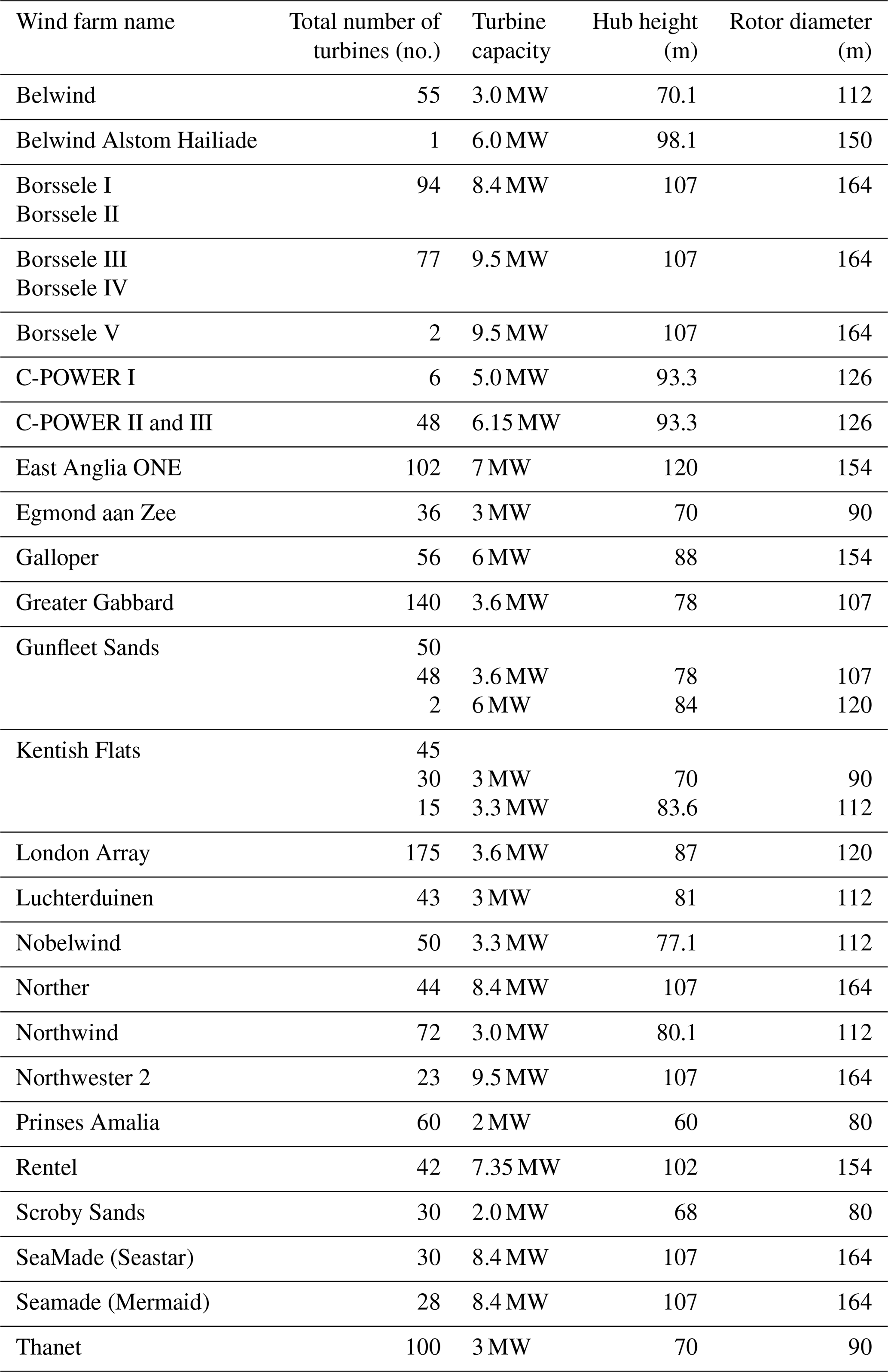
Table A1 Wind farm details, including the name of the wind farm, the number of turbines per wind farm, the turbine capacity, the turbine hub height, and turbine rotor diameter.

Appendix B: Representative year

To identify a representative simulation year, the Perkins skill score (PSS) was used. The PSS quantifies the similarity between the wind climate of an individual year and that of the full 30-year reference period, with higher values indicating a more representative year.

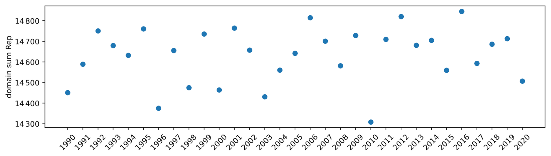
Figure B1 Sum of the representativeness per year over the area of interest, where the representativeness is based on the Perkins skill score for the wind climate between each single year and the 30-year window (Borgers et al., 2024).

Appendix C: Confidence interval for mean bias (simulation − observation)

The uncertainty calculation accounts for both the variability in the bias time series and the uncertainty associated with the measurements. For wind speed, a relative measurement uncertainty (U_m) of 3.3 % is assumed for all stations except Westhinder, where a value of 5.6 % is used. For wind direction, no measurement uncertainty is available, and thus only the model variability is considered.

The effective number of independent samples (N_eff) is estimated to account for temporal autocorrelation (10 min output) in the bias time series, as shown in Eq. (C1).

$$\begin{array}{}\text{(C1)}& N_{\text{eff}}={\displaystyle \frac{N}{\mathrm{1}+\mathrm{2}{\mathit{\rho }}_{\mathrm{1}}}}\end{array}$$

Here, N is the total number of samples, and ρ₁ is the lag-1 autocorrelation coefficient of the bias.

The total uncertainty in the mean bias (U_tot) is calculated as the quadratic sum of the uncertainty due to model variability and the uncertainty associated with the measurements, shown in Eq. (C2).

$$\begin{array}{}\text{(C2)}& U_{\text{tot}}=\sqrt{{\left({\displaystyle \frac{{\mathit{\sigma }}_{\text{bias}}}{\sqrt{N_{\text{eff}}}}}\right)}^{\mathrm{2}}+{\left({\displaystyle \frac{U_{\mathrm{m}}{\stackrel{\mathrm{‾}}{X}}_{\text{obs}}}{\sqrt{N_{\text{eff}}}}}\right)}^{\mathrm{2}}}\end{array}$$

Here, σ_bias is the standard deviation of the bias time series, and ${\stackrel{\mathrm{‾}}{X}}_{\text{obs}}$ is the mean measured value at the observation mast. The first term in Eq. (C2) represents the standard error of the mean bias due to model variability, while the second term represents the measurement uncertainty. When the measurement uncertainty is not available (e.g., for wind direction), only the first term in Eq. (C2) is used.