Annual wake impacts in and between wind farm clusters – Part 2: Comparison of WRF and fast-running engineering wake models

Wind energy is regarded as an important component for global decarbonization strategies, and the rapid expansion of offshore wind farms has led to increasingly large and closely spaced wind farm clusters. As a result, assessing wake impacts between neighboring wind farms has become increasingly important. Multiple numerical modeling approaches are available for such assessments and differ in their physical assumptions, representations of atmospheric processes, and computational cost. Numerical weather prediction models and fast-running engineering wake models are both used for long-term wake impact studies, yet they are based on different assumptions regarding atmospheric variability and wake recovery. These differences introduce uncertainty in predicted power production, and it remains unclear how consistently the different modeling approaches estimate long-term wake impacts and how sensitive these estimates are to model formulation.

Here we compare wake impacts predicted by commonly used engineering wake models with those simulated by a numerical weather prediction model (WRF), simulated in Part 1 (Porchetta et al., 2026) of this paper series, for a meteorologically representative year (2016), focusing on the planned Princess Elisabeth offshore wind farm cluster and the Belgian–Dutch wind farm cluster in the southern North Sea. We show that engineering wake models generally predict higher wind farm power production and smaller wake energy losses than WRF. Separating these losses into internal and external components reveals that external wake energy losses have a larger relative spread between modeling approaches than internal wake energy losses, particularly during summer.

By analyzing wake energy losses as a function of atmospheric stability, we demonstrate that discrepancies between modeling approaches increase under stable stratification, which occurs more frequently during summer. Under these conditions, reduced turbulent mixing leads to slower wake recovery and increased sensitivity to the wake recovery formulation. Engineering wake models that explicitly account for turbulence-dependent wake recovery show closer agreement with WRF, particularly for external wake losses. These results quantify the uncertainty associated with long-term intra-farm and farm–farm wake estimates and identify atmospheric stability as a key driver of model spread.

This paper forms the second part of a two-part study investigating wake impacts of offshore wind farms. In Part 1, wake effects induced by the planned Princess Elisabeth wind farm cluster are analyzed using WRF to characterize annual mean and sub-annual variability under atmospheric conditions. The present paper (Part 2) builds on this analysis by comparing the WRF estimates with commonly used fast-running engineering wake models, enabling a systematic assessment of differences between modeling approaches and the uncertainty associated with long-term intra-farm and farm–farm wake estimates.

1 Introduction

Driven by global decarbonization ambitions, wind energy capacity has expanded rapidly in recent years, urging for a better understanding of its interaction with its surroundings. Furthermore, because of this rapid expansion of wind energy, wind farms are larger in size and closer to each other. In densely developed regions, such as the North Sea, the interaction between neighboring wind farms, known as the farm–farm wake interaction, becomes more important. A farm wake is the region of reduced wind speed behind a wind farm that affects the power production of a wind farm located downstream (Lundquist et al., 2019; Barthelmie et al., 2010; Pryor et al., 2021; Stieren and Stevens, 2022). These farm–farm wake interactions introduce an additional source of uncertainty in wind resource assessment and energy yield estimates, which has direct impacts on wind farm development. Moreover, wake impacts are not constant in time and vary during the year, which is particularly important for operational planning, maintenance scheduling, and short-term power trading.

A variety of numerical models are used to examine these farm–farm wakes, with different models focusing on specific atmospheric scales, ranging from the microscale to the mesoscale, synoptic scales, and even global scales (Veers et al., 2019; Porté-Agel et al., 2020). Microscale numerical approaches for studying farm–farm wakes encompass a range of fidelity levels. High-fidelity computational fluid dynamics models such as large-eddy simulations (Maas and Siegfried, 2022; Stieren and Stevens, 2022) and mid-fidelity Reynolds-averaged Navier–Stokes models (van der Laan et al., 2015, 2023) are computationally more expensive, often still limiting their application to specific atmospheric conditions. On the other hand, low-fidelity, fast-running engineering wake models provide a cost-effective alternative for wake studies that can account for multiple atmospheric conditions (Nygaard et al., 2020; Nygaard and Hansen, 2016; Munters et al., 2022). Yet, they greatly simplify the underlying physics and often rely on empirical tuning, limiting their ability to fully capture the actual atmospheric conditions.

In recent years, numerical weather prediction models have been employed to study wakes (Cuevas-Figueroa et al., 2022). These models account for multiple non-uniform spatial and temporal atmospheric variables and are able to capture flow heterogeneity at the mesoscale. For wind energy purposes, these models have horizontal spatial resolutions that are typically between 1 and 3 km, which is larger than the typical inter-turbine spacings (Fischereit et al., 2022a). On some occasions, this spatial horizontal resolution can be as small as 333 m or as large as 5 km (Prosper et al., 2019). Wind farm parameterizations are used within these models to represent the effects of wind turbines that occur at the subgrid scales (Veers et al., 2019). Historically, numerical weather prediction models have not been considered the models of choice for evaluating yearly power production or wake loss estimates from wind farms due to their relatively high computational cost. However, recent advancements in computational resources have allowed these models to be applied to longer time periods (Akhtar et al., 2021; Borgers et al., 2024). In numerical weather prediction models, wakes are not explicitly prescribed. Instead, wake dynamics are determined by the atmospheric flow field, where the mean flow is explicitly resolved at the grid scale for the mesoscale model, and subgrid-scale turbulence is represented through parameterizations. In these models there are no explicit assumptions about wake propagation, recovery, or superposition, but the resolution remains insufficient to resolve intra-farm wake interactions down to the turbine scale (<1 km).

Fast-running engineering models, such as Jensen, Gauss-BPA, TurbOPark, and cumulative curl models, have been widely used to estimate the yearly production and wake losses of wind farms due to their very low computational cost (Peña et al., 2018). Although engineering wake models are fast-running compared with mesoscale models, their computational cost can still increase substantially with the number of turbines, which is becoming increasingly important for large wind farm clusters. The main limitation of engineering wake models lies in the assumptions and simplifications used and how these assumptions remain valid for large wind farms and farm–farm wakes. Engineering wake models can be categorized into bottom-up, top-down, and coupled approaches. Bottom-up models simulate wakes at turbine scale and combine individual wakes to represent farm-scale effects (Bastankhah and Porté-Agel, 2014; Katic et al., 1986). These models perform well for intra-farm wakes but often predict a faster recovery of wakes than observed for large wind farms, leading to an underestimation of farm–farm effects (Fischereit et al., 2022b). This is partly because these wake models do not represent all the boundary layer processes that control momentum replenishment and thus wake recovery in large wind farm clusters. Top-down models describe the impact of a wind farm on the atmospheric boundary layer as a whole and are better suited to capture the total momentum deficit induced by large wind farms but generally lack flow heterogeneity dependence (Emeis, 2010; Antonini and Caldeira, 2021). Coupled approaches aim to combine turbine-scale wake formulations with boundary layer information, offering improved physical consistency at the cost of increased complexity and calibration requirements (Stevens et al., 2015; Nygaard et al., 2020).

Although there have been previous comparisons between numerical weather prediction models and fast-running engineering models (Hansen et al., 2015; Fischereit et al., 2022b), they have not been conducted over an extended time period. Fischereit et al. (2022b) found that mesoscale models are able to accurately estimate the mean wind speed deficit but incur a higher error in estimating peak wind speed deficits, which can be partly attributed to their limited ability to resolve intra-farm wake effects. The same study showed that most engineering wake models perform well for intra-farm wakes but less so for farm–farm wakes, as they indicate a faster recovery of wind-speed deficits, particularly at longer downstream distances. Fischereit et al. (2022b) suggest that engineering wake models could be enhanced in estimating farm–farm wakes with the availability of more calibration data. Recently, new developments such as the TurbOPark wake model and the cumulative curl model have been proposed to reduce the underestimation of fast-running engineering models to better represent farm–farm wakes (Pedersen et al., 2022; Bay et al., 2023).

Despite these advances, it remains unclear which modeling approach (numerical weather prediction model vs. fast-running engineering wake models) provides more reliable long-term estimates of wake impacts for large offshore wind farm clusters. Since no validation data are available within the scope of this study to establish a ground truth, the objective is not to identify a single best-performing model. Instead, comparing wake predictions from different model approaches allows the uncertainty associated with farm–farm wake assessments to be quantified. Such a comparison makes it possible to assess the spread in integrated metrics, such as annual energy production and wake-induced losses, and to identify the atmospheric factors, such as wind speed, wind direction, and atmospheric stability, that drive differences between model predictions.

To address this gap, this study examines the annual mean and sub-annual variability in wake effects induced by a planned wind farm cluster on surrounding operational wind farms. Wake impacts are predicted using both a numerical weather prediction model (Part 1; Porchetta et al., 2026) and commonly used fast-running engineering wake models (Part 2). While both approaches are suitable for longer-term analyses, a systematic comparison over a full, meteorologically representative year has so far been lacking. This comparison is conducted for the planned Princess Elisabeth (PE) wind farm cluster, which will be constructed in the near future in the Belgian part of the North Sea. The year under investigation is the most meteorologically representative of the past 30 years (see Part 1). This allows for a realistic assessment of the impact of wakes on adjacent operational wind farms. This study only includes commonly used wind farm parameterization and engineering wake models using standard calibration parameters, even though some models or calibration parameters may perform better under specific conditions.

This paper constitutes Part 2 of a two-part study investigating wake impacts of offshore wind farm clusters. While Part 1 focuses on the characterization of annual mean and sub-annual wake effects using a numerical weather prediction model, the present paper (Part 2) extends this analysis by comparing numerical weather prediction results with commonly used fast-running engineering wake models. By comparing the results of these different model strategies, this study aims to quantify the spread in predicted wake impacts and to identify key drivers of model approach discrepancies, thereby providing insight into the uncertainty associated with long-term farm–farm wake assessments.

2 Material and methods

The materials and methods presented in this section are applied to the new Princess Elisabeth (PE) wind farm cluster and existing adjacent wind farms. However, the same methodology can be adapted to study other farm–farm interactions.

2.1 Study area and period

The study area and period are identical to Part 1 of this study and consist of the meteorological year 2016, modeling the new 3.5 GW Princess Elisabeth (PE) wind farm cluster of 15 MW turbines together with the existing adjacent wind farms (Fig. 1). Three configurations are considered for both numerical models: (i) a reference case without wind farms (“no WF”), (ii) only the existing wind farms (“without PE”; black dots in Fig. 1), and (iii) both the existing wind farms and the new PE wind farms (“with PE”; black and red dots in Fig. 1). In this part of the study (Part 2), we only focus on the effect of the PE wind farm cluster on the Belgian–Dutch (BE–NL) wind farm cluster. In this part of the study (Part 2) only these turbines are modeled, while all adjacent wind farms are modeled within WRF (see Part 1). The implications of this simplification are discussed in Sect. 2.3 and further evaluated in Appendix A.

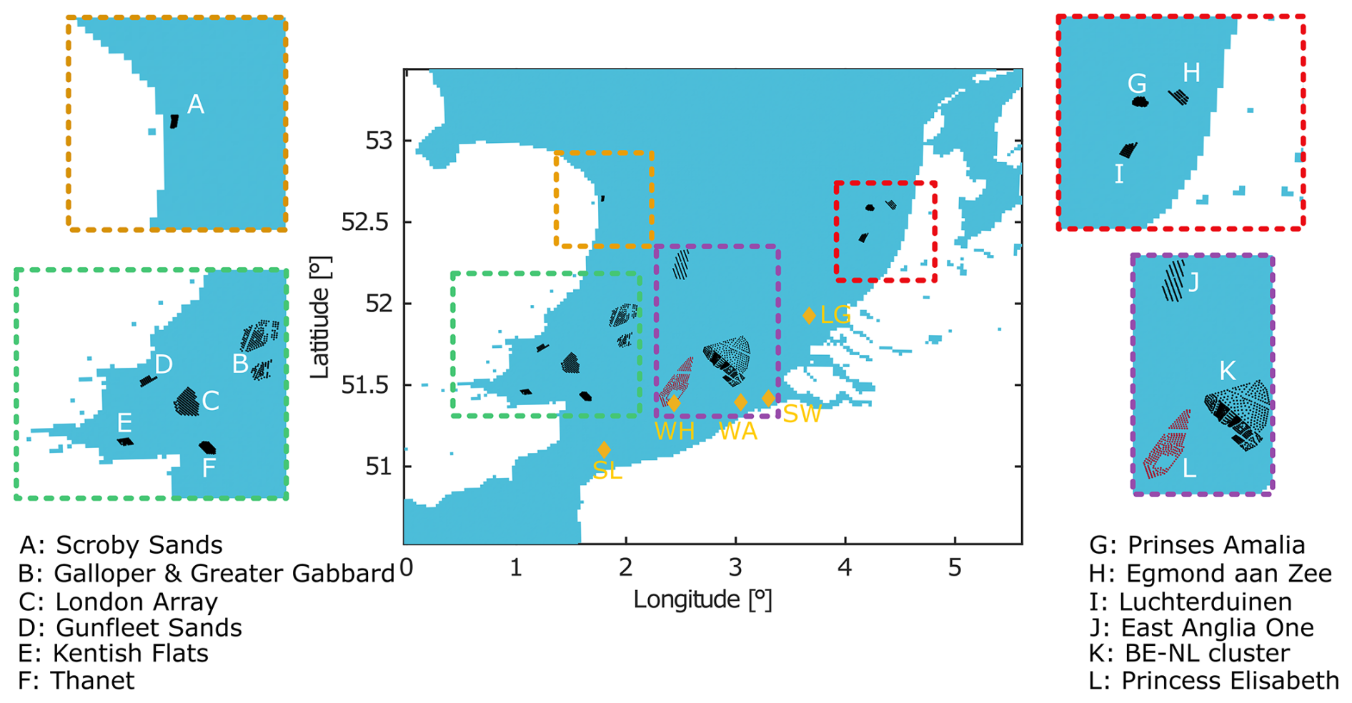
Figure 1 Location of the new Princess Elisabeth wind farms (red dots) and the existing wind farms (black dots) within the southern North Sea. Yellow diamonds show the location of measurement masts used for the validation of the WRF setup in Part 1 of this study.

2.2 Numerical models

2.2.1 WRF

Simulations are performed using the Weather Research and Forecasting (WRF) model v4.3 (Skamarock et al., 2008). The same model configuration as in the companion study (Part 1) is employed, consisting of three nested domains with horizontal grid spacings of 18, 6, and 2 km and boundary conditions from the ERA5 reanalysis. Wind farm effects are represented using the Fitch parameterization (Fitch et al., 2012). Three simulations are considered: a reference simulation without wind farms (no WF), a simulation including the existing wind farms (without PE), and a simulation including both the existing wind farms and the Princess Elisabeth wind farm cluster (with PE). Further details of the model configuration are provided in Part 1 of this study.

2.2.2 Fast-running engineering wake models

The engineering wake modeling is conducted using FLORIS v4.4 (NatLabRockies, 2025), an open-source wake modeling framework developed by the National Laboratory of the Rockies (NLR), formerly the National Renewable Energy Laboratory (NREL). FLORIS provides state-of-the-art engineering wake modeling capabilities, including tools for annual energy production estimations and wake steering optimization.

An ensemble of commonly used classical and more recent wake deficit models is employed in this study to provide a comparison with the numerical weather prediction model WRF.

As a classical bottom-up engineering approach, the Jensen model (Katic et al., 1986) is included. The Jensen model assumes that the wake expands as a cone with a fixed linear expansion constant, k_w, independent of the ambient turbulence intensity (TI). In this study, two values are considered for the wake decay coefficient – (1) a “standard” value k_w=0.04 and (2) a reduced value k_w=0.02 – following recent recommendations based on a large-scale benchmark over an entire fleet of offshore wind farms (Nygaard et al., 2022). We note that stability-dependent formulations for the wake spreading rate in the Jensen model have been proposed but are not applied in this study to keep the number of wake model representations constrained (Peña et al., 2016).

The Gaussian wake model proposed by Bastankhah and Porté-Agel (2014), hereafter referred to as Gauss-BPA, is included as a more recent engineering wake formulation. In this model, the wake is represented by a Gaussian velocity deficit whose width depends linearly on the ambient turbulence intensity, TI_amb, through a wake growth rate defined as

$$\begin{array}{}\text{(1)}& k^{*}=k_{\mathrm{a}}{\mathrm{TI}}_{\mathrm{amb}}+k_{\mathrm{b}}.\end{array}$$

The Gauss-BPA model is used with its out-of-the-box calibration parameters, namely k_a=0.38 and k_b=0.004.

In addition to these conventional engineering models, the TurbOPark model (Pedersen et al., 2022) is considered. TurbOPark was specifically developed to mitigate excessive wake recovery in long-distance wake development, including farm–farm interactions, by means of a modified turbulence recovery scheme. The model incorporates a non-linear wake expansion that is sensitive to the local turbulence intensity and its downstream decay, given by

$$\begin{array}{}\text{(2)}& {\displaystyle \frac{\mathrm{d}{\mathit{\sigma }}_{\text{w}}\left(x\right)}{\mathrm{d}x}}=A\mathrm{TI}\left(x\right)=A\sqrt{{\mathrm{TI}}_{\text{amb}}^{\mathrm{2}}+{\mathrm{TI}}_{\text{w}}^{\mathrm{2}}\left(x\right)},\end{array}$$

where σ_w denotes the characteristic wake width, and A is a calibration constant. The local turbulence intensity TI(x) at a downstream distance x from the turbine is computed as the quadratic sum of the ambient turbulence intensity TI_amb and the wake-added turbulence intensity TI_w(x), whose evolution is modeled following Frandsen (2007). The TurbOPark model is run using the default expansion coefficient A=0.04 as well as the value A=0.06, as proposed by van der Laan et al. (2023), who show that the default parameter tends to overestimate wake effects.

Finally, the cumulative curl model (Bay et al., 2023) is included as a wake model specifically designed for large wind farm arrays. The cumulative curl model builds upon the Gauss–curl hybrid (GCH) model (King et al., 2021) by incorporating cumulative wake deflection and recovery mechanisms that account for the superposition of multiple upstream wakes. It introduces a set of streamwise counter-rotating vortices generated by yaw misalignment, which are accumulated across turbines to represent the combined effect of wake steering. Unlike the GCH model, which superimposes individual wakes, the cumulative curl model computes the combined wake effect using a momentum-conserving formulation proposed by Bastankhah et al. (2021). The wake velocity deficit is modeled using a Gaussian profile, with centerline deflection and recovery effects evolving cumulatively across the turbine array. The cumulative curl model retains the deflection formulation from GCH while adding secondary steering and yaw-induced recovery effects driven by the accumulated vortex structures. The cumulative curl model is run using default parameters.

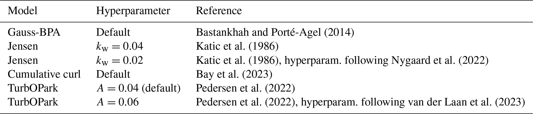
For all cases, except the cumulative curl model that uses its built-in superposition scheme, wake overlap is handled using the sum-of-squares freestream velocity superposition method. Turbines are aligned with the mean flow direction, and therefore no additional wake deflection model is applied. A summary of the deficit models used in this study is provided in Table 1.

Bastankhah and Porté-Agel (2014)Katic et al. (1986)Katic et al. (1986)Nygaard et al. (2022)Bay et al. (2023)Pedersen et al. (2022)Pedersen et al. (2022)van der Laan et al. (2023)

Table 1 Overview of the engineering wake models used in this study.

FLORIS simulations are driven by meteorological conditions extracted from the no-WF WRF simulations for the entire year 2016 (see Part 1). These conditions include wind speed, wind direction, and turbulence intensity (TI). The no-WF velocity field is provided to FLORIS using two different inflow setups. The first setup assumes horizontally homogeneous inflow and retrieves the wind speed from a single probe point located at the geographic center of the BE–NL cluster at an altitude of 96 m. In contrast, the heterogeneous inflow configuration accounts for spatial variability in the incoming flow, arising from coastal gradients or large-scale synoptic structures.

In the heterogeneous configuration, FLORIS’s built-in implementation described by Farrell et al. (2021) is used. Specifically, the no-WF velocity field at 96 m height is extracted at the WRF grid points and fed to FLORIS. For each wind turbine, FLORIS initializes the local inflow wind speed by performing a linear barycentric interpolation of the WRF wind speed field. Wake velocities downstream of each turbine are then computed following the standard FLORIS wake modeling approach but using this locally interpolated inflow wind speed as the initial condition. No vertical interpolation is applied since both vertical wind shear and veer are omitted in the present study.

A portion of the engineering wake model simulations assume a time-varying TI estimated based on the no-WF WRF data following Larsén (2024), which proposes using the Kaimal turbulence spectrum to approximate the wind speed component variances, σ_u, σ_v, and σ_w, at given heights and wind speeds. Empirical ratios between σ_u and other components then allow the TKE extracted from WRF to be transformed into the along-wind standard deviation. The ambient TI can then be estimated as

$$\begin{array}{}\text{(3)}& {\text{TI}}_{\mathrm{amb}}={\displaystyle \frac{{\mathit{\sigma }}_u}{\stackrel{\mathrm{‾}}{U}}}={\displaystyle \frac{\mathrm{1}}{\stackrel{\mathrm{‾}}{U}}}\sqrt{{\displaystyle \frac{\mathrm{2}\text{TKE}}{\mathrm{1}+{\mathit{\alpha }}^{-\mathrm{1}}+{\mathit{\beta }}^{-\mathrm{1}}}}},\end{array}$$

with $\stackrel{\mathrm{‾}}{U}$, the mean wind speed over the averaging period at the height of interest, and α and β, empirical height- and wind-speed-dependent coefficients determined based on Kaimal turbulence spectra. However, integrating this TI correction strategy was shown not to significantly affect the estimated TI compared to the classical approach, for which α=1 and β=1.

Four different FLORIS simulation setups are subsequently considered.

• Homogeneous FLORIS with fixed TI. A time-varying and spatially homogeneous wind field is assumed in FLORIS, constructed from the wind speed and direction at 96 m altitude at the geographic center of the BE–NL wind farm cluster, taken from the no-WF WRF simulation (Part 1). Turbulence intensity is fixed in space and time at 6 %, a typical value for the offshore North Sea area.

• Homogeneous FLORIS with varying TI. A time-varying and spatially homogeneous wind field and TI are assumed in FLORIS, constructed from the wind speed, wind direction, and TI at 96 m altitude at the geographic center of the BE–NL wind farm cluster, taken from the no-WF WRF simulation (Part 1). This setup aims at evaluating whether incorporating temporal variability in ambient turbulence resulting from changes in different atmospheric conditions improves the representation of wake recovery.

• Heterogeneous FLORIS with fixed TI. A time-varying and spatially heterogeneous wind speed field is assumed in FLORIS, constructed from the wind speed at 96 m altitude taken from the no-WF WRF simulation (Part 1). Wind direction is kept spatially homogeneous and time-varying, constructed from the no-WF WRF simulation at 96 m altitude at the geographic center of the BE–NL wind farm cluster (Part 1). Turbulence intensity is fixed in space and time at 6 %, a typical value for the offshore North Sea area.

• Heterogeneous FLORIS with varying TI. A time-varying and spatially heterogeneous wind speed field is assumed in FLORIS, constructed from the wind speed at 96 m altitude taken from the no-WF WRF simulation (Part 1). Wind direction is kept spatially homogeneous and time-varying, constructed from the no-WF WRF simulation at 96 m altitude at the geographic center of the BE–NL wind farm cluster (Part 1). A time-varying and spatially homogeneous TI is assumed, constructed from TI at 96 m altitude at the geographic center of the BE–NL wind farm cluster, taken from the no-WF WRF simulation (Part 1).

All four setups of the engineering wake models are run in a time series mode with a 30 min resolution for 1 full year (2016 selected in this study based on analysis in Part 1), where each simulation time step is treated as quasi-steady and independent. Consequently, the model does not account for wake advection or temporal effects in wake propagation contrary to WRF. As noted previously, not all wind farms in the North Sea are modeled; for the engineering models used in this study only those belonging to the BE–NL and PE wind farm cluster are included. This reduced domain of not including all North Sea wind farms allows for the simulation of 12 cases (3 layouts – no WF, with PE, and without PE similar to WRF – combined with 4 input setups described above) capturing the dominant inter-farm wake losses of the PE wind farm cluster on the BE–NL wind farm cluster.

To facilitate comparison between WRF and the engineering wake models, envelope ranges are shown throughout this study. In each case, the solid line represents the mean estimate of the engineering wake models and/or model configurations considered in the analysis, while the envelope is defined by the corresponding minimum and maximum estimates. The envelope therefore represents the spread associated with these models and configurations. For figures showing differences relative to WRF, the differences are first computed for each engineering wake model or model configuration individually relative to WRF, after which the mean and envelope are determined from these differences.

2.3 Wake energy losses

Wake energy losses in Part 2 are evaluated using the same conceptual framework as in Part 1 (Sect. 2.5), distinguishing between internal, total (internal + external), and external wake energy losses. Wake energy losses are defined as percentage energy losses computed from temporally averaged turbine power production relative to a reference case without wind farms (no WF). Depending on the analysis, the averaging period may correspond to the full simulation year, individual months, or subsets of the data conditioned on wind speed, wind direction, atmospheric stability, or a combination thereof. To enable a direct comparison between WRF and the engineering wake models, all wake energy losses are normalized using the same reference energy obtained from the no-WF WRF simulation.

Small differences between the wake energy losses of WRF reported in Part 1 and those obtained in Part 2 arise from differences in temporal resolution. While the WRF analysis in Part 1 uses 10 min output, the engineering wake model simulations in Part 2 operate on 30 min mean conditions. For consistency, the WRF power output used in Part 2 is therefore aggregated to 30 min resolution by averaging consecutive 10 min samples. This difference in temporal aggregation can lead to small deviations in the estimated wake losses (e.g., WRF internal wake losses in Part 1 and Part 2 of 42.01±0.28 % and 41.46±0.24 %, respectively) but does not affect the comparison between WRF and the engineering wake models presented in this study.

Note that the definition of internal wake energy losses is not strictly identical between the WRF simulations (Part 1) and the engineering wake models (Part 2). WRF-derived internal wake losses may contain a small contribution from neighboring existing wind farms, whereas the engineering wake models only account for wake effects generated within the BE–NL cluster. Additional sensitivity analyses indicate that this contribution is minor and does not affect the conclusions of the model comparison (Appendix A).

2.4 Stability classification

Atmospheric stability is classified using the Monin–Obukhov length (L) extracted from the WRF surface layer scheme (Part 1). The classification follows the scheme of Van Wijk et al. (1990), consistent with Part 1 (Sect. 2.4). Five stability classes are considered: very stable (VS; $\mathrm{0}<L<\mathrm{200}$ m), stable (S; $\mathrm{200}\le L<\mathrm{1000}$ m), near neutral (NN; $\left|L\right|\ge \mathrm{1000}$ m), unstable (U; $-\mathrm{1000}<L\le -\mathrm{200}$ m), and very unstable (VU; $-\mathrm{200}<L<\mathrm{0}$ m).

3 Results and discussion

Results are presented either at the wind farm level or at the grid cell level; the latter refers to individual horizontal grid cells of the WRF model (Part 1). As multiple turbines may be located within a single grid cell, all wind farm quantities evaluated at the grid cell level (e.g., wake energy losses) represent aggregated model results rather than turbine-resolved values. Since the engineering wake model results are computed at the turbine level, these results are aggregated to the WRF grid cell to enable a direct comparison.

3.1 Spatiotemporally averaged power

We next quantify the differences between the engineering wake models and their various setups (homogeneous or heterogeneous inflow, fixed or varying turbulence intensity) relative to WRF. Prior to this comparison, a verification of the no-WF cases was performed to ensure consistent use of WRF inputs in the engineering wake models (Appendix B). Since no observational data are available within the scope of this study, the aim is not to identify the best-performing model, but rather to assess the spread between models. To this end, we use three performance statistics: the coefficient of determination R², the root-mean-square error (RMSE), and the mean bias. The bias expresses the average difference between the power estimated by the engineering wake models and WRF, where a positive bias indicates that the engineering model predicts higher power than WRF, whereas a negative bias indicates a lower power. In contrast, RMSE reflects the typical size of the deviations between the two time series, and R² describes how well the engineering model captures the temporal variability seen in WRF.

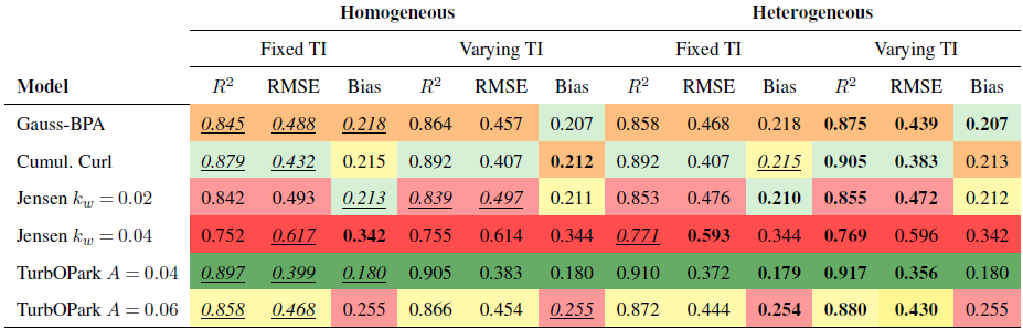
Table 2 summarizes these statistics for all engineering wake models and the different setups for the simulations without the PE cluster. It should be noted that all engineering wake models and their different setups exhibit a positive bias relative to WRF, ranging from approximately 0.18 GW for TurbOPark (A=0.04) to 0.342 GW for Jensen (k_w=0.04). Table 2 shows that, among the examined engineering wake models, TurbOPark with a spreading parameter of A=0.04 provides the closest agreement with WRF, with RMSE values as low as 0.356 GW, a bias of 0.18 GW, and R² values up to 0.917. By comparison, the Jensen model with k_w=0.04 shows the largest deviations from WRF across all metrics, with an RMSE value of 0.617 GW, bias of 0.342 GW, and R² value 0.752. The same behavior is observed in the simulations including the PE cluster (Table C1).

When comparing the different model setups (homogeneous or heterogeneous inflow, fixed or varying turbulence intensity) in Table 2, the heterogeneous inflow combined with varying turbulence intensity generally produces the closest agreement with WRF. However, the relative importance of inflow conditions and turbulence intensity depends on both the performance metric and the engineering wake model. For RMSE and R², improvements associated with inflow conditions typically amount to reductions of approximately 0.02–0.03 GW in RMSE and increases of about 0.01–0.02 in R² when comparing homogeneous and heterogeneous inflow conditions at both fixed and varying turbulence intensity. In contrast, the impact of turbulence intensity on RMSE and R² is more model-dependent: for Gauss-BPA, switching from fixed to varying turbulence intensity under both homogeneous and heterogeneous inflow conditions reduces RMSE by approximately 0.03 GW, exceeding the corresponding improvement due to inflow conditions, whereas for the Jensen model the effect of turbulence intensity is negligible, and improvements are primarily driven by inflow conditions.

For the mean bias, the sensitivity to the setup is model-dependent. Gauss-BPA shows a strong dependence on turbulence intensity, with a reduction in bias of approximately 0.01 GW when switching from fixed to varying turbulence intensity, while the bias change is small going from homogeneous to heterogeneous inflow. In contrast, TurbOPark shows an almost invariant bias across all setups, with differences below 0.001 GW, indicating that its bias is largely controlled by the wake model formulation itself. The Jensen model exhibits a weak sensitivity of the bias to both inflow conditions and turbulence intensity, consistent with its formulation, in which wake recovery does not explicitly depend on turbulence intensity.

Differences between engineering wake model formulations reach a maximum of 0.26 GW in RMSE, 0.17 in R², and 0.16 GW in bias relative to WRF, whereas variations associated with inflow conditions or turbulence intensity within a given engineering wake model remain below 0.03 GW in RMSE, 0.02 in R², and 0.01 GW in bias. This indicates that the engineering wake model formulation constitutes the dominant source of variability in comparison to WRF, while setup choices provide a secondary influence on model performance.

Based on these findings, TurbOPark with A=0.04 is used as the representative engineering wake model in subsequent analyses when a single wake model is considered. This choice does not imply that TurbOPark provides the most accurate representation of wake effects, given that no observational validation data are available, and WRF cannot be regarded as a ground truth. Rather, TurbOPark is selected because it exhibits the closest overall agreement with WRF within a consistent modeling framework, providing a single reference for further comparative analysis. Likewise, the setup with heterogeneous inflow with varying turbulence intensity is selected as the preferred configuration for the remainder of the study when a single setup is considered.

While calibration of engineering wake model parameters could potentially further improve agreement with WRF in terms of the spatiotemporally averaged metrics presented above, such calibration would not necessarily improve agreement at individual time steps. The time-dependent behavior of the different modeling approaches is therefore investigated next.

Table 2 R², RMSE [GW], and mean bias [GW] for the different engineering wake models (without PE) compared against WRF, shown for the four model setups: homogeneous, fixed TI; homogeneous, varying TI: heterogeneous, fixed TI: and heterogeneous, varying TI. Color shading highlights relative performance ranking of the engineering wake models within each metric column (R², RMSE, and mean bias for a given inflow setup) ranging from dark red (worst) to light red, orange, yellow, light green, and dark green (best). Typographic emphasis (best: bold; worst: italic and underlined) highlights the relative performance of the different inflow setups within a given engineering wake model.

3.2 Time-dependent behavior

3.2.1 Total farm power

The temporal evolution of the total BE–NL wind farm cluster power for WRF and the engineering wake models in the simulations without PE is shown in Fig. 2. The time series further confirms the results obtained from the spatiotemporally averaged comparison in Sect. 3.1. Over the year the engineering wake models estimate higher total wind farm power compared to WRF. This indicates smaller wake losses in the engineering models relative to WRF, consistent with previous studies showing that WRF with the wind farm parameterization of Fitch et al. (2012) produces stronger wake deficits and reduced power production compared to engineering wake models (Fischereit et al., 2022b, 2025). Quantitatively, the WRF power estimates fall within the envelope of the engineering wake models for 40 % of the simulated hours, while for the remaining 60 % of the time WRF lies outside this range, indicating periods of stronger disagreement between modeling approaches.

The results for the simulations with PE (Fig. D1) also show that the engineering wake models estimate higher total power compared to WRF. In this case, WRF power estimates fall within the envelope of the engineering wake models for 38 % of the simulated hours, while for 62 % of the time WRF lies outside this range. This increased fraction of hours suggests that the inclusion of the PE cluster increases the differences between the modeling approaches. This could originate from the fact that engineering wake models are primarily tuned for intra-farm wakes and may be less suited to represent farm–farm wake interactions without additional tuning (Nygaard et al., 2020; Fischereit et al., 2022b).

Furthermore, also consistent with the spatiotemporally averaged comparison in Sect. 3.1, the temporal comparison in Fig. 2 shows that differences between wake engineering models are larger than differences by different model setups. This is depicted by the narrow spread between different setups of a given engineering wake model (Fig. 2b, d, f) compared to the larger spread between the envelope of the engineering wake models (Fig. 2a, c, e).

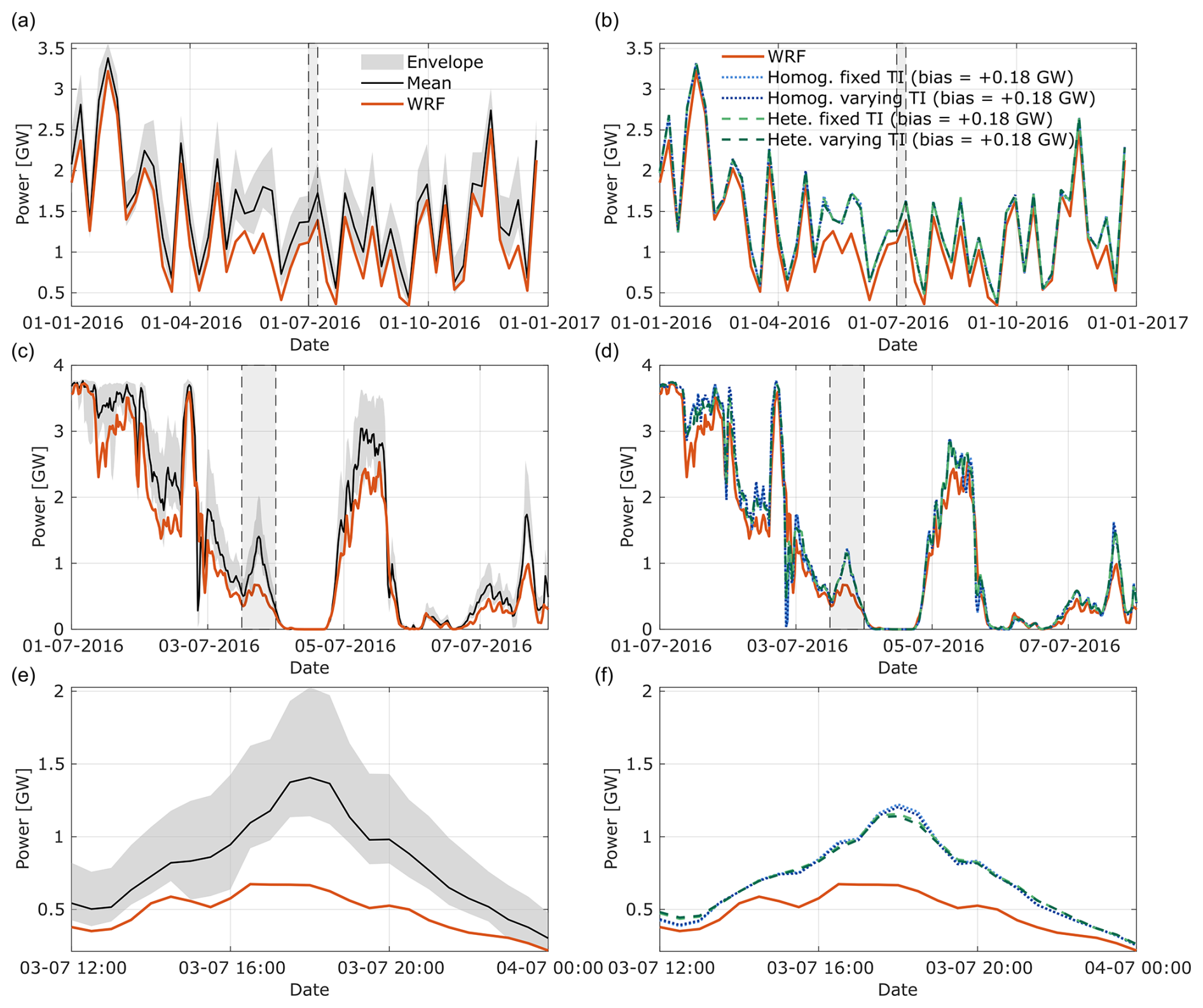
Figure 2 Total power (GW) for the BE–NL offshore wind farm cluster for simulations without PE. Shown are WRF, the mean and envelope of all engineering models (a, c, e), and the different configurations of TurbOPark with induction factor A=0.04 (b, d, f). The top row (a, b) shows weekly averages computed from 30 min data, the middle row (c, d) shows a 1-week zoom (1–7 July 2016) at 30 min resolution, and the bottom row (e, f) shows a 12 h zoom (3 July 2016) also at 30 min resolution. The zoom periods were selected to show periods with the largest differences between WRF and the engineering wake models. The dashed box shows the time period zoom within the longer time series. The bias is calculated as the engineering wake model minus WRF.

3.2.2 Grid cell power

A grid cell refers to an individual horizontal WRF model grid cell (for details of simulation setup see Part 1) and represents the aggregated response of all turbines located within that cell. The same spatial aggregation is applied to the engineering wake model results. Grid cell power at three locations (Fig. 3a) is compared between the engineering wake models and WRF (without PE), corresponding to the farm center, a coastal site, and a more offshore site. Similar results are found for the with-PE investigation (Fig. D1).

In contrast to the total farm power time series (Fig. 2), the grid cell power time series (Fig. 3) exhibits larger differences between the homogeneous and heterogeneous setups. At the farm center (Fig. 3d, e), both configurations yield identical results, as expected. At the coastal location (Fig. 3b, c), introducing heterogeneity improves agreement with WRF, reducing the bias from 0.9 to 0.7 MW. In contrast, at the offshore location (Fig. 3f, g), the bias increases from 1.0 to 1.1 MW. To interpret these differences, it is useful to distinguish between wake biases and wind speed gradient biases, the latter being in the homogeneous inflow setups.

The wake bias shows higher power production estimates by the engineering wake models compared to WRF for both homogeneous and heterogeneous inflow setups. In addition, the homogeneous configuration is affected by a wind speed gradient bias because the inflow is derived from wind conditions at a single grid point (at the spatial center of the wind farm) and does not represent the spatial wind speed gradients resolved by WRF. Depending on the local wind speed, this wind speed gradient bias can partially compensate or increase the wake bias when the engineering models are compared with WRF.

At the coastal grid cell, the homogeneous inflow has a higher wind speed compared to the WRF grid cell wind speed, which adds to the wake bias and yields a larger total power bias. Introducing heterogeneity reduces this larger inflow relative to WRF, thereby reducing the power bias. At the offshore grid cell, the homogeneous inflow has lower wind speeds compared to the WRF grid cell wind speed, which compensates the wake bias and leads to a smaller apparent power bias. Accounting for heterogeneity corrects the inflow toward the WRF wind speed. This removes the compensating inflow error present in the homogeneous configuration, revealing the full wake bias and therefore increasing the total power bias compared to WRF. These changes in bias thus reflect the presence or removal of wind gradient bias compensation in comparison to WRF.

Although bias response to the inclusion of inflow heterogeneity differs between regions, the spatiotemporally aggregated comparison in Sect. 3.1 shows smaller biases compared to WRF for the heterogeneous inflow setup. Accounting for heterogeneity reduces inflow biases associated with wind speed gradients, while local increases or decreases in bias partially cancel when integrated over the full wind farm and year. As a result, the total bias is reduced compared to the homogeneous inflow setup, even though heterogeneity can locally increase the bias at individual grid cells. We nonetheless note that including heterogeneity is expected to improve the physical realism of the modeling setup. Even in cases where the apparent bias increases, the heterogeneous configuration remains more faithful to the underlying flow physics, as it better represents spatial variability in the inflow. The remaining discrepancies therefore primarily reflect differences in wake model response between the WRF-based inflow and the engineering wake model implementation.

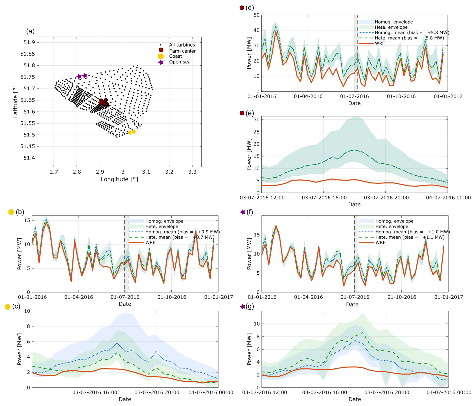
Figure 3 Grid cell power output (MW) at three representative locations within the BE–NL wind farm cluster for simulations without PE. Panel (a) shows the locations of the selected grid cells, representing the farm center (circle) as well as coastal (pentagon) and open-sea (star) regions. Panels (d), (b), and (f) show weekly averages computed from 30 min data, while panels (e), (c), and (g) show a 12 h zoom on 3 July 2016 at 30 min resolution. Shown are WRF (without PE) and the mean and envelope of all engineering wake models grouped by homogeneous and heterogeneous setups. The dashed box indicates the zoomed period within the full time series. Bias is defined as the engineering wake model power minus WRF power.

3.3 Internal and external wake energy losses

3.3.1 Spatiotemporally averaged wake energy losses

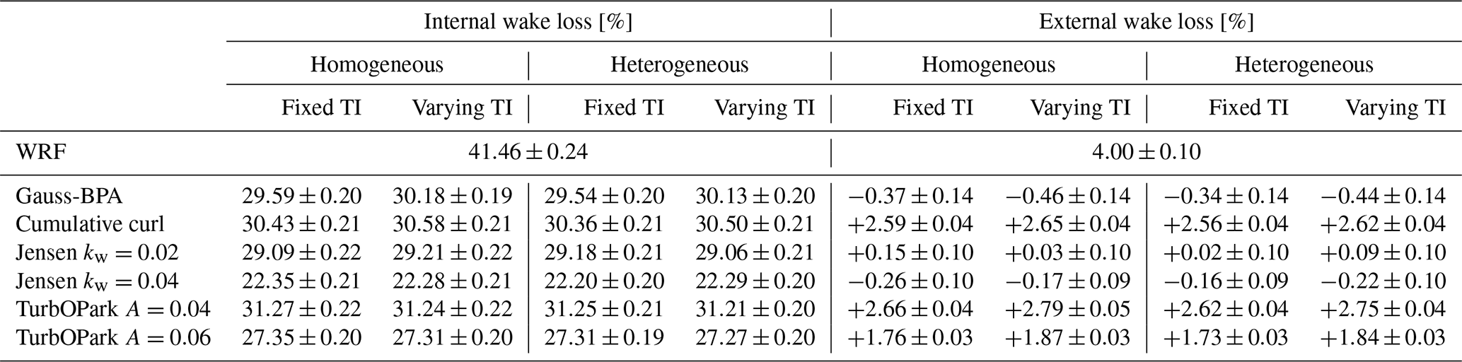
Beyond the total power metrics discussed in Sect. 3.1, the separation of internal and external wake energy losses in Table 3 makes it possible to investigate the contributions of intra-farm and farm–farm wake effects explicitly. Table 3 shows, as presented earlier, that differences between different engineering wake models and WRF are larger compared to the different inflow setups within a given engineering wake model and WRF. For the latter, variations between homogeneous and heterogeneous and between fixed and varying TI are small and mostly within the uncertainty range.

For the internal wake energy losses, WRF predicts larger losses (41.46±0.24 %) than any engineering wake model across all inflow setups, which range from approximately 22 % for the Jensen model with k_w=0.04 to about 31 % for TurbOPark with A=0.04, the latter providing the closest agreement with WRF. These results are consistent with the spatiotemporally averaged power comparison in Sect. 3.1, where internal wake effects dominate the overall power differences between modeling approaches.

Also for the external wake losses, differences between the engineering wake models and WRF are larger than the differences from different inflow setups within a given engineering wake model. While WRF yields an external wake loss of 4.00±0.10 %, the engineering wake models span from near-zero or slightly negative losses for Gauss-BPA and Jensen to approximately 2.5 % for the cumulative curl and TurbOPark models. This range indicates that external wake energy loss estimates of the engineering models relative to WRF are primarily controlled by the wake model formulation. In particular, models explicitly designed to represent long-range and cumulative wake interactions, such as TurbOPark and cumulative curl, produce external wake losses that are closer to WRF than the more classical engineering formulations (Nygaard et al., 2020). A previous study by Fischereit et al. (2022b) has shown that WRF with Fitch et al. (2012) can provide a more realistic representation of farm–farm wake effects under specific atmospheric conditions compared to engineering wake models (Fischereit et al., 2022b). While these findings cannot be directly generalized to the full-year simulations analyzed here, the closer agreement of TurbOPark and cumulative curl with WRF suggests that these models may be more suitable for representing farm–farm wake interactions than the other engineering wake models considered in this study.

Comparing internal and external wake energy losses shows that although the absolute inter-model spread is larger for internal wake losses (22 %–31 %), the relative inter-model variability is larger for external wake losses, which range from negligible or slightly negative values to about 2.5 %. This highlights that the farm–farm wake estimates are more sensitive to the wake model formulation than to the estimates of intra-farm wake effects.

The slightly negative external wake energy losses obtained for Jensen with k_w=0.04 and Gauss-BPA should not be interpreted as physically meaningful negative wake losses. These values occur only for engineering wake models predicting very weak external wake effects. Further investigation is required to better understand the origin of these slightly negative values.

Table 3 Spatiotemporal mean internal and external wake losses for WRF and the engineering wake models. Uncertainties denote the half-width of the 95 % confidence interval obtained from 1000 bootstrap resamples. All values are given in percent.

3.3.2 Spatial patterns of wake energy losses

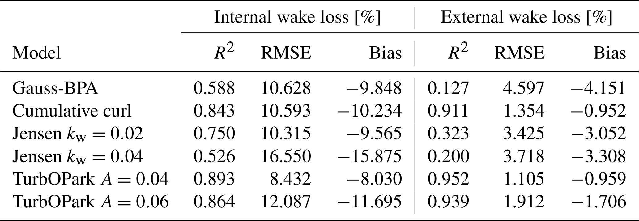
In Fig. 4, the yearly averaged results for WRF and the different engineering wake models using the heterogeneous, varying TI setup are shown, together with the differences (in percentage points) in wake energy loss between each engineering model and WRF. Both the internal (Fig. 4a–m) and external (Fig. 4n–z) wake energy losses are presented together with the performance metrics compared to WRF in Table 4.

For the internal wake losses, all engineering wake models show enhanced wake energy losses in the interior of the wind farm. While several models show comparable spatiotemporal mean internal wake losses in Table 3 (e.g., 30.13 % for Gauss-BPA and 30.50 % for cumulative curl), their spatial agreement with WRF differs substantially (R²=0.588 vs. 0.893 from Table 4). In particular, the Gauss-BPA and Jensen with k_w=0.04 models have larger deviations and thus lower spatial correspondence with WRF. These results indicate that similar spatiotemporally averaged internal wake energy losses can arise even if the spatial distributions are different. This difference may partly be related to local wind farm density, as internal wake losses are largest in the densely packed interior of the wind farm. TurbOPark and cumulative curl reproduce both the magnitude (Table 3) and the spatial pattern (Table 4) of the internal wake losses more consistently compared to WRF.

For the external wake energy losses, the spatial agreement between WRF and the engineering wake models exhibits a larger spread than for the internal wake energy losses, with R² values ranging from 0.127 for Gauss-BPA to 0.952 for TurbOPark with A=0.04 (Table 4). Only TurbOPark and cumulative curl reproduce spatial patterns that are similar to WRF, whereas the other engineering wake models show weak spatial correspondence and are not able to represent the farm–farm wake. This was also represented by the spatiotemporal results in Table 3.

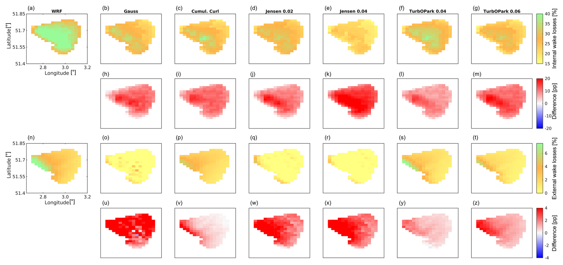
Figure 4 Temporal mean internal (a–g) and external (n–r) wake energy losses for WRF and all engineering wake models with the heterogeneous, varying TI inflow setup. The second (h–m) and fourth (u–z) rows show the corresponding differences in wake energy losses, expressed in percentage points, between each engineering wake model and the WRF simulation for internal and external wake losses, respectively.

Table 4 R², RMSE (pp), and mean bias (pp) for the different engineering wake models compared against WRF, shown for the heterogeneous with varying TI inflow setup. Bias is defined as engineering model − WRF.

3.3.3 Monthly farm wake energy losses variations

Figures 5 and 6 show the monthly variation in internal and external wake energy losses from the engineering wake models, expressed as percentage point (pp) differences compared to WRF. Results are shown for three groups: (a) comparison of inflow conditions, (b) TurbOPark A=0.04 configurations, and (c) heterogeneous inflow with varying TI for all engineering wake models. For both the internal and external wake energy losses a seasonal pattern is present, with larger differences between the modeling approaches during summer than during winter months. This is also visible in the time series of total wind farm power and grid cell power, respectively (Figs. 2 and 3).

For the internal wake energy losses (Fig. 5c), wintertime model approach differences range from 4 to 20 pp, increasing to 19–31 pp during the summer months, with differences between engineering wake models themselves being larger compared to differences from inflow setups. For the external wake energy losses (Fig. 6c), differences between modeling approaches range from 1 to 6 pp in winter and increase to 4–11 pp in summer. Although these absolute differences are smaller than those found for the internal wake energy losses (Fig. 5c), the external wake energy losses predicted by WRF are also considerably smaller, resulting in larger relative differences between the modeling approaches for external wake energy losses. In addition, the spread between wake model formulations is more pronounced for external than for internal wake losses, reflecting the higher sensitivity of farm–farm wake interactions to engineering wake model formulations. Some slight negative external wake energy losses are observed during some periods and for certain models, consistent with earlier findings; this needs further investigation.

In Part 1 of this study, both internal and external wake energy losses show seasonal variability, linked to changes in wind speed and atmospheric stability. The results presented here in Figs. 5 and 6 further show that these summer conditions are associated with increased differences between WRF and engineering wake model estimates (modeling approaches) for both internal and external wake energy losses. During summer, lower wind speeds and more frequent stable stratification lead to reduced turbulent mixing and slower wake recovery, conditions that are accounted for in WRF through stability-dependent planetary boundary layer parameterizations but are only indirectly represented in engineering wake models. Consequently, these differences between modeling approaches persist downstream and amplify deviations in wake energy losses. Engineering wake models such as TurbOPark and the cumulative curl model, which incorporate turbulence-dependent wake recovery and wake expansion, tend to show closer agreement with WRF under these conditions. In addition, turbines operate less frequently in above-rated conditions during summer than in winter. Since wake effects are reduced when turbines operate above rated wind speed, agreement between WRF and engineering wake models is generally higher in winter, further contributing to the increased spread observed in summer. The increased spread observed in summer therefore suggests that improved representation of atmospheric stability and its impact on wake recovery in engineering wake models is key to reducing discrepancies with WRF.

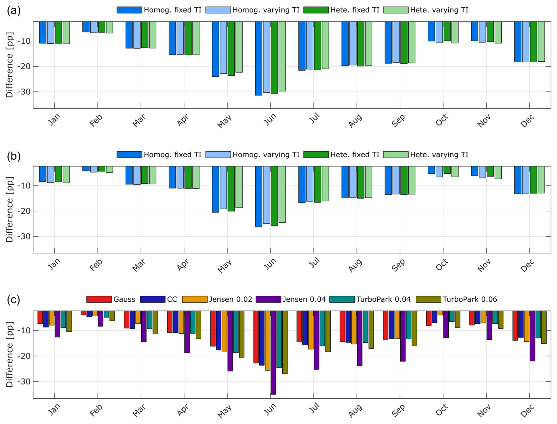
Figure 5 Monthly internal wake energy loss difference compared to WRF (in percentage points). (a) All engineering wake models clustered by setup (homogeneous, fixed TI; homogeneous, varying TI; heterogeneous, fixed TI; and heterogeneous, varying TI). (b) TurbOPark (A=0.04) results for the same four inflow setups. (c) All engineering wake models corresponding to the heterogeneous, varying TI setup.

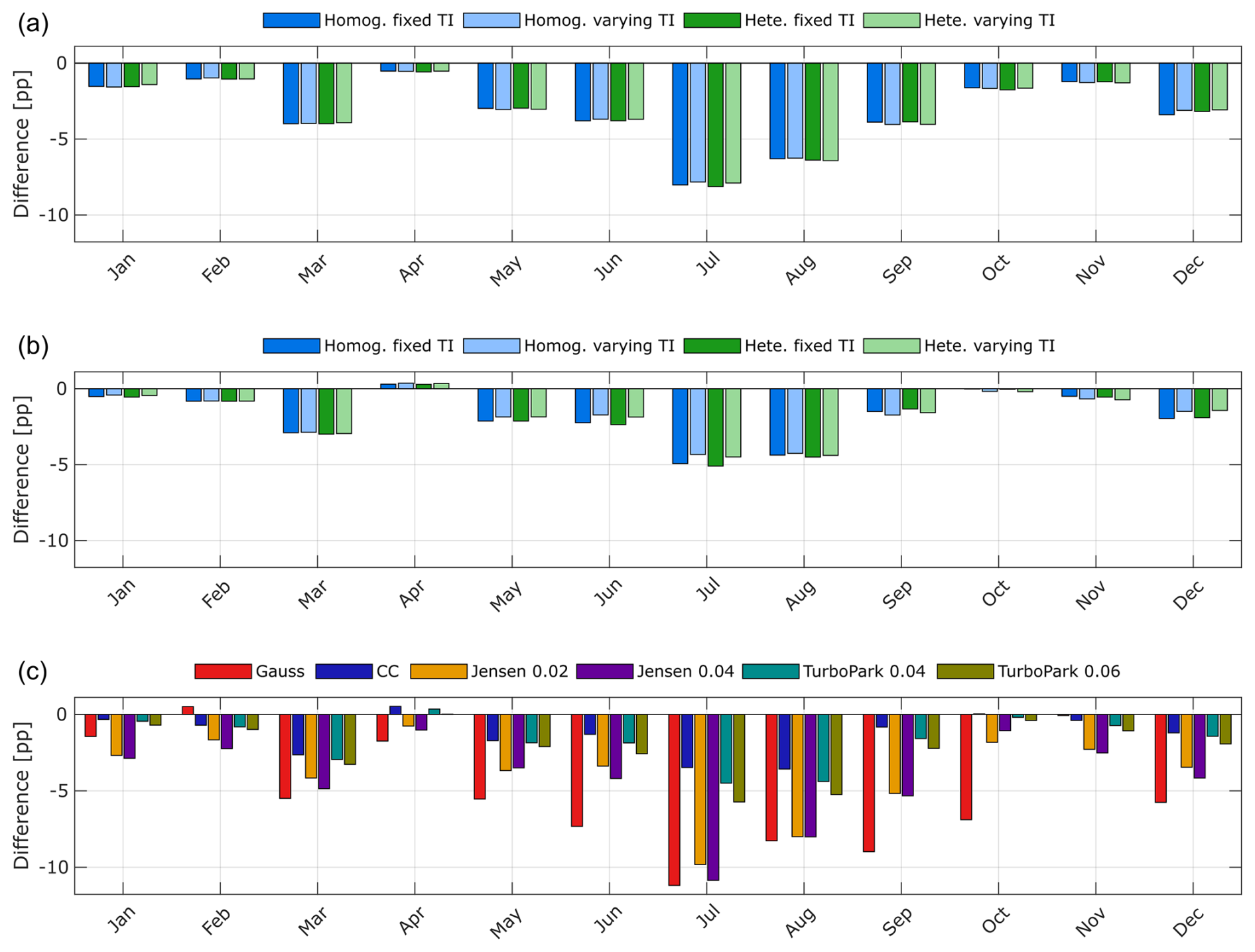
Figure 6 Monthly external wake energy loss difference compared to WRF (in percentage points). (a) All engineering wake models clustered by setup (homogeneous, fixed TI; homogeneous, varying TI; heterogeneous, fixed TI; and heterogeneous, varying TI). (b) TurbOPark (A=0.04) results for the same four inflow setups. (c) All engineering wake models corresponding to the heterogeneous, varying TI setup.

3.3.4 Variation with atmospheric stability

Building on the seasonal analysis from Sect. 3.3.3, an explicit investigation on how the internal and external wake energy losses from the different modeling approaches behave across atmospheric stability classes is discussed next (Fig. 7). How these energy losses depend on atmospheric stability classes for WRF has been discussed in Sect. 3.3 and 3.4 in Part 1 of this study. In general, Fig. 7 shows that the differences between the modeling approaches are primarily driven by the wake modeling formulation rather than by the inflow conditions.

For the internal wake energy losses with heterogeneous, varying TI inflow conditions (Fig. 7a), the uncertainty ranges associated with the different engineering wake models show partial overlap with the WRF modeling approach, especially during unstable conditions. However, differences between modeling approaches still remain present during stable conditions. This confirms that there is an increased sensitivity of wake recovery to stability under low turbulence regimes. Under higher-turbulence conditions, turbulent mixing accelerates wake recovery, leading to closer agreement between the modeling approaches. The same can be observed from Fig. 7b, which isolates the effect of inflow conditions for the TurbOPark model (A=0.04). In both Fig. 7a and b, the uncertainty ranges of the engineering wake models and of the different inflow conditions, respectively, largely overlap, making it difficult to identify a single modeling approach or inflow configuration that is consistently closer to WRF for internal wake losses.

For the external wake energy losses when comparing the different modeling approaches under heterogeneous, varying TI inflow conditions (Fig. 7c), overlap between uncertainty ranges is observed across multiple stability classes and not only under unstable conditions, which was the case for internal wake energy losses. However, in contrast to the internal wake energy losses, the engineering wake models themselves no longer overlap consistently over all stability classes, indicating a stronger sensitivity of external wake losses to the underlying wake formulation. In particular, models that explicitly account for turbulence-dependent wake recovery and expansion, such as TurbOPark and the cumulative curl model, show closer agreement with WRF across stability classes.

When isolating the effect of inflow conditions for the TurbOPark model (Fig. 7d), the uncertainty ranges associated with the different inflow configurations overlap with each other, similarly to the internal wake energy losses (Fig. 7b). Nevertheless, a slightly closer agreement with WRF is found for varying TI inflow conditions compared to fixed TI inflow conditions for stable atmospheric conditions.

Overall, this analysis provides a physical explanation for the seasonal patterns discussed in Sect. 3.3.3, where larger differences between modeling approaches were observed during summer. The increased occurrence of stable atmospheric conditions in summer enhances the sensitivity of wake recovery to the specific wake formulation, particularly for external wakes. As a result, discrepancies between WRF and engineering wake models, and among the engineering models themselves, become more pronounced under these conditions, whereas during periods dominated by unstable stratification the enhanced turbulent mixing leads to closer agreement across modeling approaches.

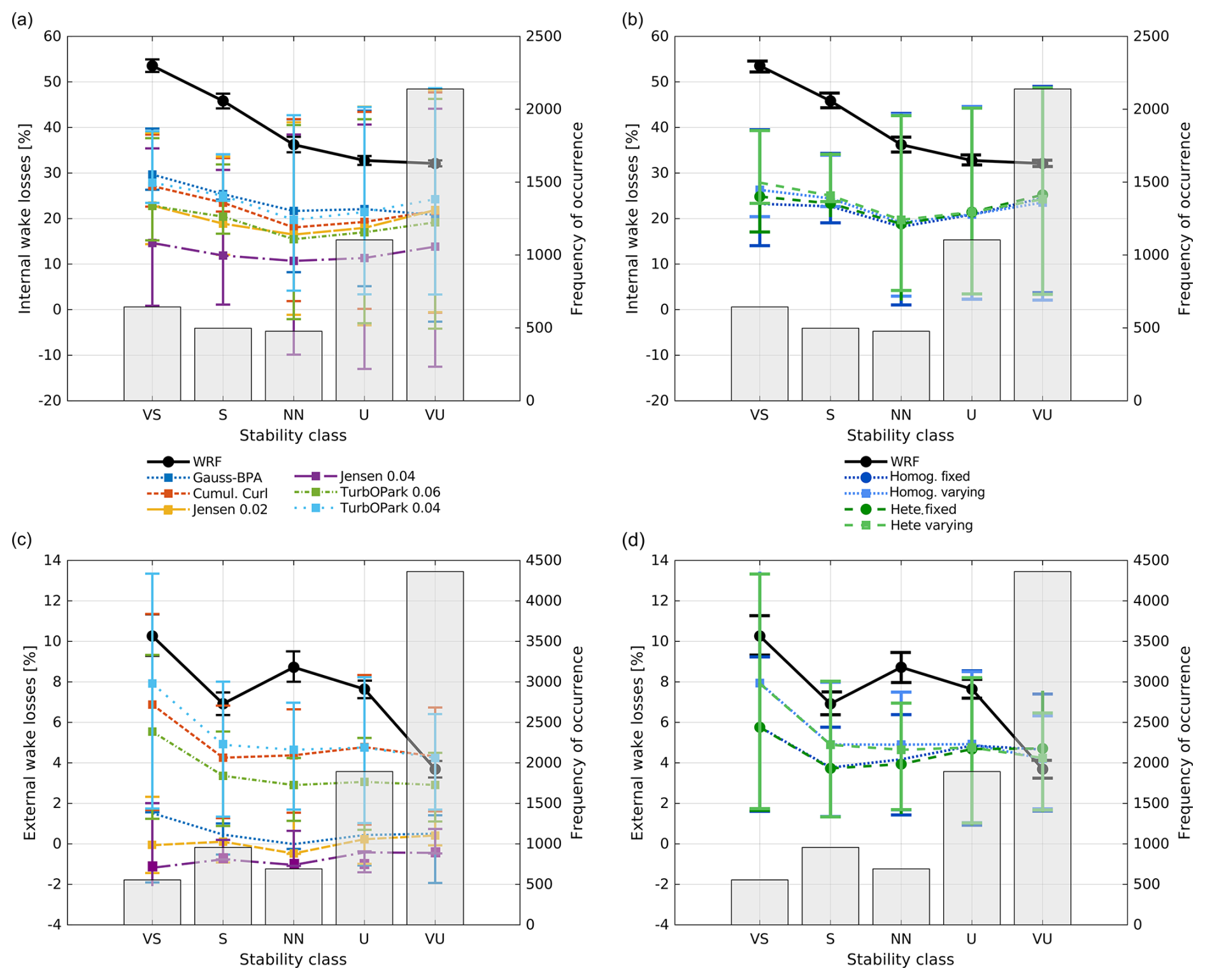
Figure 7 Spatiotemporal conditional averages of wake energy losses by atmospheric stability class (VS: very stable; S: stable; NN: near-neutral; U: unstable; VU: very unstable). (a, b) Internal wake energy losses for wind speeds between 10 and 15 m s⁻¹. (c, d) External wake losses for wind directions from 193–317°. Lines show engineering wake models for heterogeneous inflow and varying TI and WRF: (a, c) all models, (b, d) TurbOPark (A=0.04) for all inflow setups and WRF. Bars indicate the frequency of occurrence of each stability class. The error bars represent a 95 % confidence interval obtained via bootstrapping with 1000 resamples.

3.4 Flow field

Two flow field snapshots are examined (Fig. 8), one case in which the flow can be considered quasi-steady and another in which the flow is strongly transient. We compare the velocity fields (wind speed and direction) generated by the TurbOPark model (A=0.04, heterogeneous inflow with varying TI) with those produced by WRF for both situations. In Fig. 9, we observe that the first snapshot selected (15 March 2016) demonstrates a relatively steady behavior of both the wind speed and wind direction with a slow ramp-up in wind power. The resulting uncertainty envelopes remain quite narrow for both time series. In contrast, the second selected case (8 November 2016) depicts much wider uncertainty envelopes associated with a strong variability in the mean wind, especially regarding wind direction.

In the steady case (15 March 2016), both the spatial velocity fields (Fig. 8a, b) and the time series (Fig. 9a) demonstrate consistent behavior. The WRF and TurbOPark flow fields exhibit similar velocity patterns: wake propagation signatures are comparable in both models, while the background velocity field in FLORIS also appears to be in good agreement with WRF. This spatial agreement is reflected in the temporal evolution of the power time series, and the power production predicted by TurbOPark shows good correlation with WRF throughout the period. Although TurbOPark systematically predicts higher power due to faster wake recovery, both models capture comparable temporal trends, confirming that the quasi-steady flow assumption is valid in this case.

In contrast, the transient case (8 November 2016) exhibits fundamentally different behavior. As a steady-state model, FLORIS assumes that wakes propagate instantaneously across the whole domain along the wind direction measured at the central probing location of the wind farm. As a consequence, the wakes appear as coherent flow structures. In WRF, however, no such coherent wake patterns can be identified because of the strong flow heterogeneity and rapid temporal evolution. In addition, the inflow velocity field used to drive TurbOPark (i.e., the no-WF WRF velocity field) differs substantially from the velocity field simulated by WRF when the wind farm is included, particularly during the transient event (Figs. 8c, d and 9b). For the steady case, the flow far from the wind farm remains broadly similar between FLORIS and WRF, indicating that the farm primarily affects the flow through its wake while having a limited impact on the surrounding large-scale flow field. In contrast, during the unsteady case, significant differences are observed even far from the farm. This suggests a stronger interaction between wind farm wakes and the atmospheric flow during transient conditions, for example through farm-induced blockage effects or changes in boundary layer mixing. As a result, the no-WF WRF field used to drive FLORIS may no longer represent the actual inflow conditions experienced by the farm. A quantitative attribution of these mechanisms would require a dedicated comparison between no-WF and with(out)-PE WRF simulations during transient periods, which is beyond the scope of the present study.

This incapacity to account for the temporal evolution of wakes is inherent to the steady nature of the typical engineering wake models used in this study. The engineering wake models in this study rely on steady, analytical formulations and do not resolve time-dependent atmospheric boundary layer dynamics, advection, or turbulence transport. WRF solves the unsteady governing equations and explicitly represents atmospheric transport processes, thereby capturing the spatiotemporal evolution of flow structures and their impact on power generation.

To assess the specific impact of these dynamically evolving conditions, a wind direction unsteadiness flag (WD_flag) is introduced to identify periods of strong directional variability. The flag is activated when the difference between the local wind direction at the wind farm probing location and the domain-averaged wind direction exceeds a predefined threshold of 30°.

The annual time series are then analyzed for periods where WD_flag=1 and where turbines are operating, assuming a minimum wind-speed cutoff. This analysis indicates that such strongly transient conditions are rare, accounting for only approximately 2 % of the analyzed year. This confirms that engineering wake models should exhibit good agreement with WRF for the vast majority of operational conditions. Additionally, it is worth noting that turbines are often curtailed or shut down during these transient events, further limiting the practical impact of discrepancies observed in transient cases.

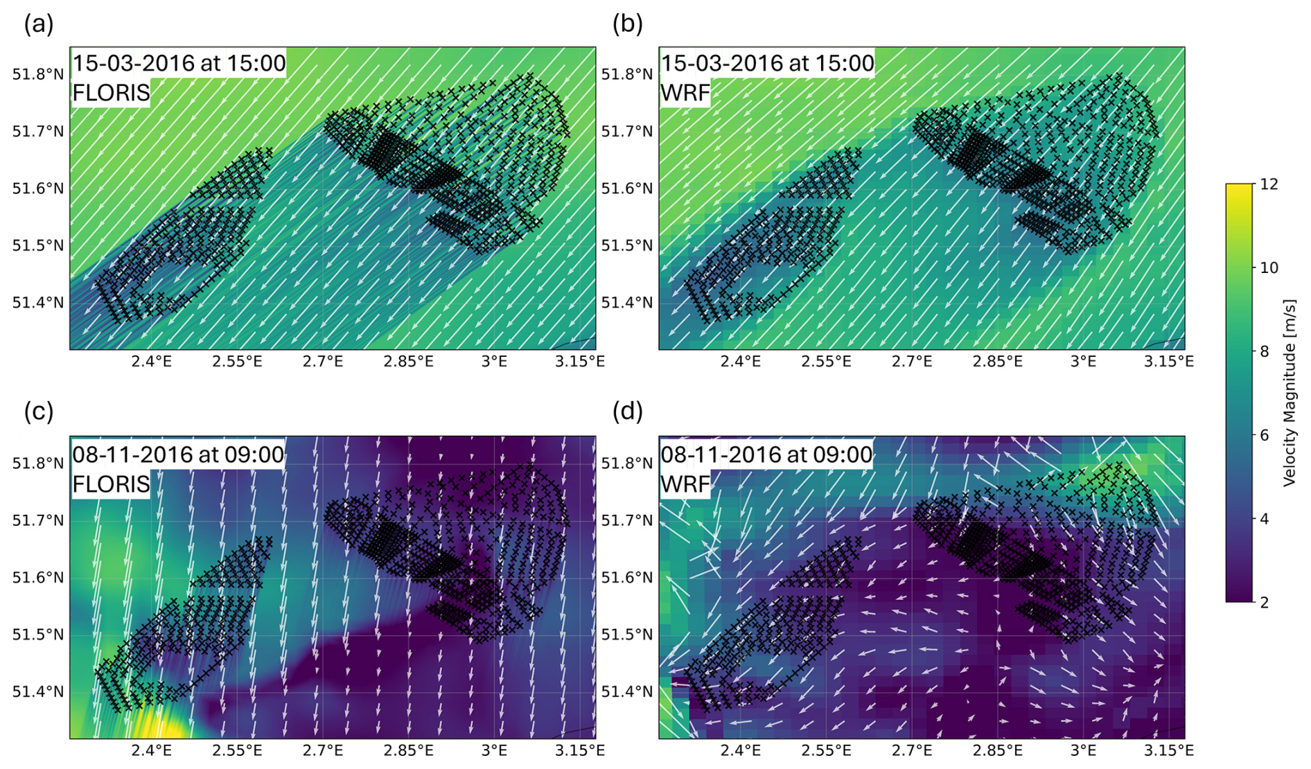
Figure 8 The velocity field for the TurbOPark A=0.04 model with varying TI (a, c) and corresponding WRF velocity field (b, d) for a steady case (15 March 2016 at 15:00) (a, b) and a transient case (8 November 2016 at 09:00) (c, d). Arrows indicate wind vectors and are shown using the same scale in all panels.

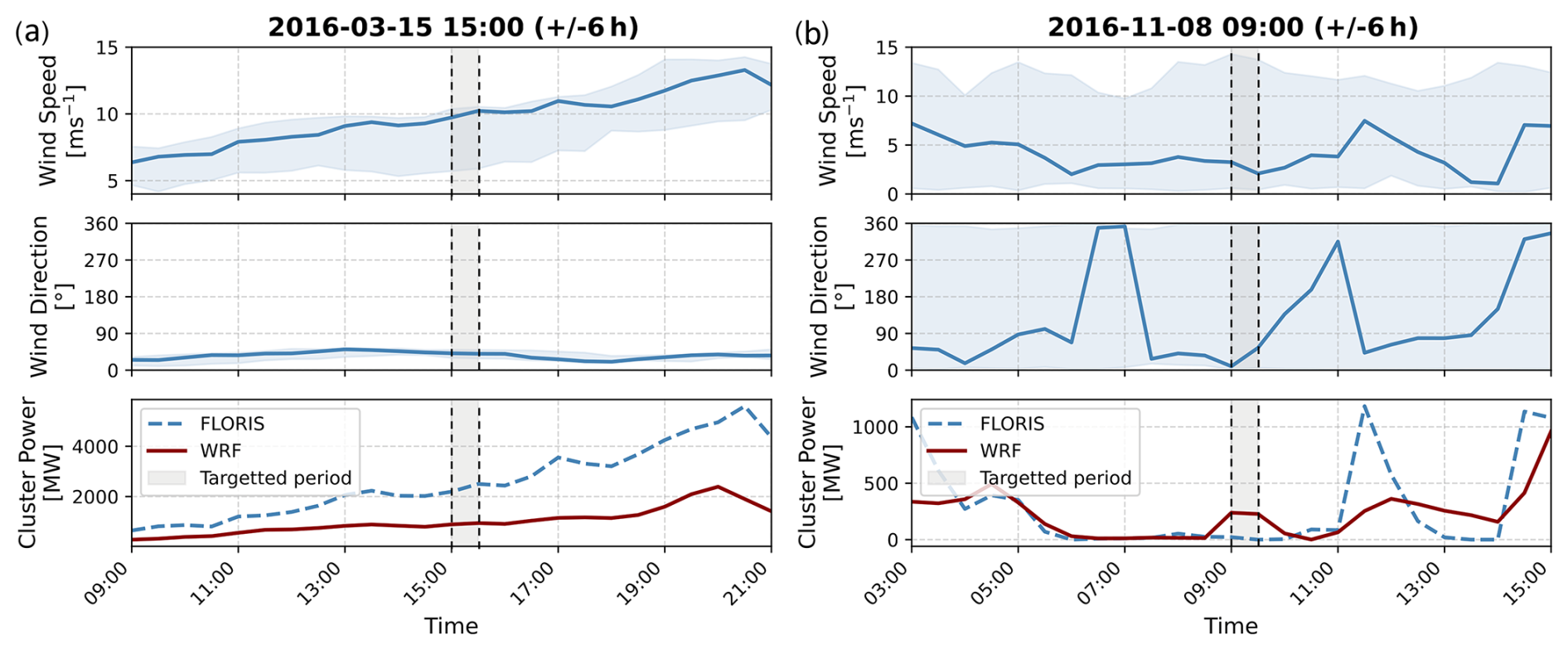
Figure 9 Time series of wind speed, wind direction, and cluster power output for WRF and TurbOPark A=0.04 (heterogeneous, varying TI) for a steady case on 15 March 2016 (a) and a strongly transient case on 8 November 2016 (b), shown over a ±6 h window around 15:00. The shaded blue area indicates lower/upper bounds of wind speed/direction across the WRF domain within the wind farm bounds. The gray area indicates the timestamp at which the snapshots of Fig. 8 were retrieved.

4 Conclusions

This study investigates how wake losses of an offshore wind farm cluster depend on the modeling approach, motivated by the lack of systematic, year-long comparisons between numerical weather prediction models and fast running engineering wake models. By analyzing a meteorologically representative year for the planned Princess Elisabeth wind farm cluster and the existing BE–NL wind farm cluster and comparing wake impacts simulated with WRF (Part 1) and commonly used engineering wake models (Part 2), the current work provides a framework to evaluate the spread in predicted wake effects at both the farm and farm–farm scale for both modeling approaches.

Engineering wake models (with different inflow setups) are compared against WRF for total wind farm power production. In general, engineering wake models predict higher power production and therefore smaller wake losses compared to WRF. Differences arising from the choice of engineering wake model are larger than those due to inflow setup, indicating that model formulation has a stronger influence on total farm power estimates than the specification of inflow conditions. Among the considered engineering wake models, TurbOPark with A=0.04 shows the closest agreement with WRF, and the inflow setup that more closely agrees with WRF is the heterogeneous inflow and varying turbulence intensity (TI).

Including inflow heterogeneity at the grid cell level can locally appear to reduce agreement with WRF; however, this effect is caused by bias compensation. Specifically, wind speed gradient bias (between WRF and the engineering wake model) offset overestimations of power production inherent to the engineering wake models, leading to an apparent improvement in agreement at specific locations. When considered in a spatially and temporally averaged sense, heterogeneous inflow configurations show a closer agreement with WRF.

Separating wake losses into internal and external wake energy losses indicates additional differences between the two modeling approaches (WRF vs. engineering wake models). For both losses, differences between engineering wake models are larger than differences associated with inflow setup when comparing to WRF. External wake energy loss estimates have a larger spread between modeling approaches than internal wake energy losses, reflecting the higher sensitivity of farm–farm interactions to engineering wake models. Engineering wake models that account for turbulence intensity variations, such as TurbOPark and the cumulative curl model, tend to show closer agreement with WRF and better reproduce the spatial patterns of wake effects. In contrast, engineering wake models with similar spatiotemporally averaged internal wake energy loss estimates can still exhibit weaker spatial correspondence with WRF, highlighting that agreement in spatiotemporally averaged losses does not mean that the internal wake energy spatial structure is captured.

Seasonal variations in wake losses are present across both modeling approaches, with larger differences during summer than winter. In summer there are lower wind speeds and more stable atmospheric conditions (Part 1), under which wake recovery is reduced, and the sensitivity of engineering wake model estimates to wake recovery is increased. Although external wake energy losses are smaller in absolute magnitude compared to internal wake energy losses, the relative deviations from WRF are larger, particularly during summer, because the external wake losses themselves are comparatively small. The stability class analysis shows indeed that this seasonal behavior is linked to stable atmospheric conditions, under which differences between modeling approaches systematically increase. This confirms that atmospheric stability is a dominant physical mechanism governing the spread of wake energy loss estimates, explaining why discrepancies between modeling approaches are largest during summer and why models with an explicit turbulence-dependent wake recovery show closer agreement with WRF, especially for external wake interactions.

The flow field comparison depicts certain conditions under which differences between the modeling approaches arise. For quasi-steady flow situations, TurbOPark A=0.04 reproduces the velocity deficit patterns of WRF. In contrast, under strongly transient inflow conditions with strong changes in wind direction, the steady-state assumptions used by engineering wake models limit their ability to capture the dynamically evolving flow structures present in WRF, which causes larger differences between the modeling approaches. However, such transient conditions occur infrequently, suggesting that the impact is limited for long-term wake studies.

While this comparison between modeling approaches provides insight into the spread of long-term wake estimates and what drives them, targeted validation against long-term observations will be required to determine which modeling approaches most realistically represent intra-farm and farm–farm interactions.

Appendix A: Impact of surrounding North Sea wind farms on internal wake loss estimates

To assess whether the different treatment of surrounding wind farms in WRF and the engineering wake models affects the comparison of internal wake losses, an additional set of FLORIS simulations was performed in which all North Sea wind farms included in the WRF simulations were modeled. The results were compared against the reduced baseline configuration used throughout this paper, in which only the BE–NL and PE clusters are included. The reduced configuration contains 572 turbines, while the full North Sea configuration contains 1504 turbines.

The power loss in the BE–NL cluster attributed to the additional surrounding wind farms is defined as

$$\begin{array}{}\text{(A1)}& \mathrm{\Delta }{P}_{\mathrm{red}}={\displaystyle \frac{P_{\mathrm{red}}-P_{\mathrm{NS}}}{P_{\mathrm{red}}}}\times \mathrm{100}\mathit{\%},\end{array}$$

where P_red is the BE–NL cluster power obtained with the reduced configuration, and P_NS is the BE–NL cluster power obtained when all North Sea wind farms are included. Positive values of ΔP_red indicate that the omitted surrounding wind farms introduce additional wake losses not captured by the reduced configuration.

Figure A1 shows ΔP_red as a function of wind direction for an inflow wind speed of 8 m s⁻¹, chosen as a worst-case scenario to maximize wake impacts. Only the homogeneous FLORIS configuration with fixed turbulence intensity is considered. As expected, the impact of the additional wind farms is negligible for wind directions between approximately 0 and 230°, for which no major wind farms are located upstream of the BE–NL cluster. For westerly to northwesterly directions (∼240–350°), corresponding to inflow from UK wind farm clusters, ΔP_red reaches up to 1.85 % for TurbOPark (A=0.04) and 0.93 % for TurbOPark (A=0.06) while remaining below 0.17 % for the Gauss-BPA and Jensen models. Since these directions are not dominant in the southern North Sea wind climate, the annual-average contribution is expected to be substantially smaller.

These results indicate that the omission of surrounding North Sea wind farms in the reduced engineering model configuration introduces only a limited bias in the estimated wake losses of the BE–NL cluster. Consequently, the differences between WRF and the engineering wake models reported in this paper cannot be explained solely by the different treatment of surrounding wind farms, and the comparison of internal wake losses remains meaningful despite the slightly different definitions.

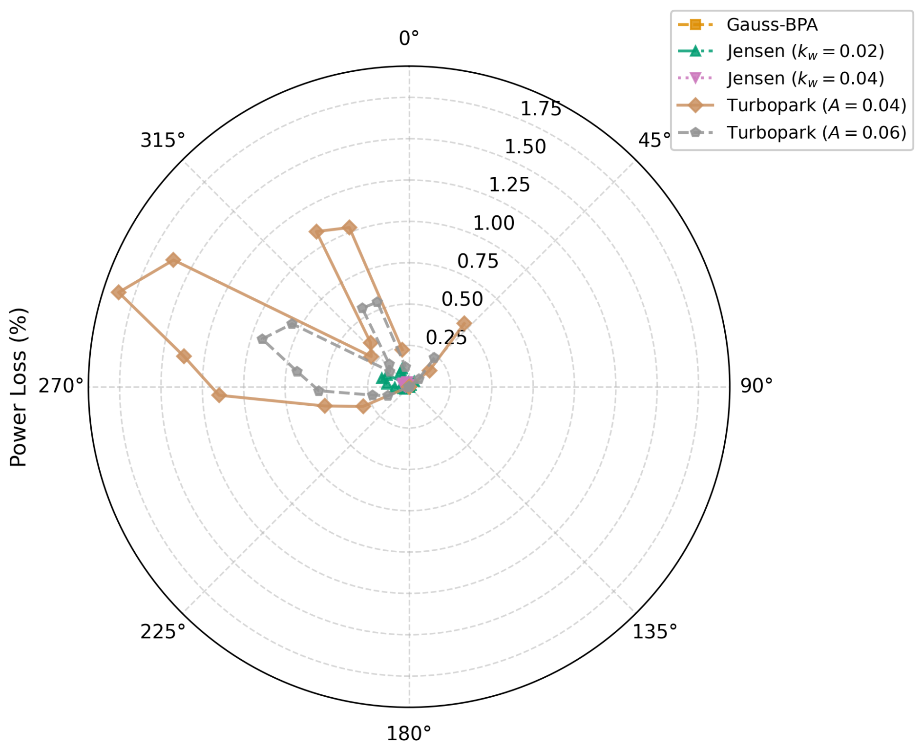
Figure A1 Additional external power loss ΔP_red in the BE–NL cluster resulting from the inclusion of all surrounding North Sea wind farms in FLORIS, shown as a function of wind direction at 8 m s⁻¹ for five engineering wake models under homogeneous inflow with fixed TI. The cumulative curl model is omitted due to excessive computational cost on the full-domain configuration.

Appendix B: Verification engineering wake models and WRF

To ensure consistent results between the different modeling approaches (i.e., engineering wake models and WRF), the no-WF simulations from both approaches are compared. In the no-WF simulations, wind turbines are not explicitly included; instead, the power production is calculated from the wind speed using the turbine power curve. Figure B1 compares the total BE–NL cluster power estimated by the engineering models with the power estimated by WRF. Overall we can see that the cluster power estimated by WRF and the engineering wake models are in close agreement, thus validating that all inputs from WRF are fed consistently to the engineering wake model setups. As expected, the homogeneous engineering setups exhibit a substantially larger spread compared to the heterogenous setups. Incorporating spatial heterogeneity in the engineering models yields improved agreement with WRF. Indeed, the no-WF wind field is not uniform and can vary substantially over large distances, e.g., due to the presence of coastal gradients or mesoscale weather systems. The remaining discrepancies between the heterogeneous setups of the engineering wake models and WRF arise from differences in how the inflow wind speed is defined for the engineering wake models. Here, the wind speed at 96 m is used, whereas in WRF the power is calculated using the wind speed at hub height, which is different from turbine to turbine. This mismatch in reference height explains the minimal remaining differences.

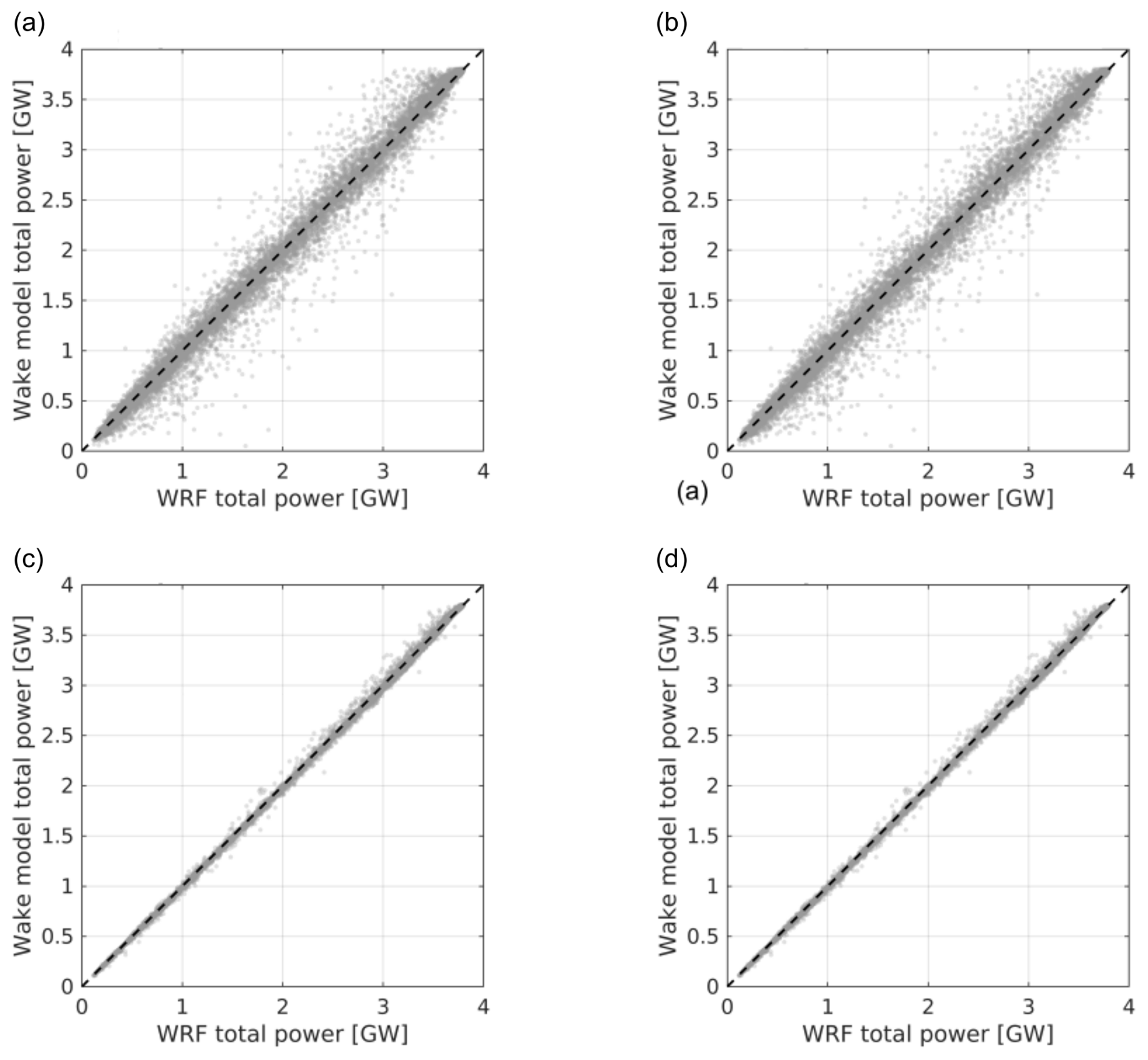
Figure B1 Total BE–NL wind farm cluster power for the no-WF simulation compared between WRF and the four engineering wake model setups: (a) homogeneous with fixed TI (slope = 1.001, R²=0.990), (b) homogeneous with varying TI (slope = 1.001, R²=0.990), (c) heterogeneous with fixed TI (slope = 1.000, R²=0.998), and (d) heterogeneous with varying TI (slope = 1.000, R²=0.998). The dashed line represents the 1:1 line.

Appendix C: Spatiotemporally averaged power

Table C1 R², RMSE [GW], and mean bias [GW] for the different engineering wake models (with PE) compared against WRF, shown for the four model setups: homogeneous, fixed TI; homogeneous, varying TI; heterogeneous, fixed TI; and heterogeneous, varying TI. Color shading highlights relative performance ranking of the engineering wake models within each metric column (R², RMSE, and mean bias for a given inflow setup) ranging from dark red (worst) to light red, orange, yellow, light green, and dark green (best). Typographic emphasis (best: bold; worst: italic and underlined) highlights the relative performance of the different inflow setups within a given engineering wake model.

Appendix D: Time-dependent behavior

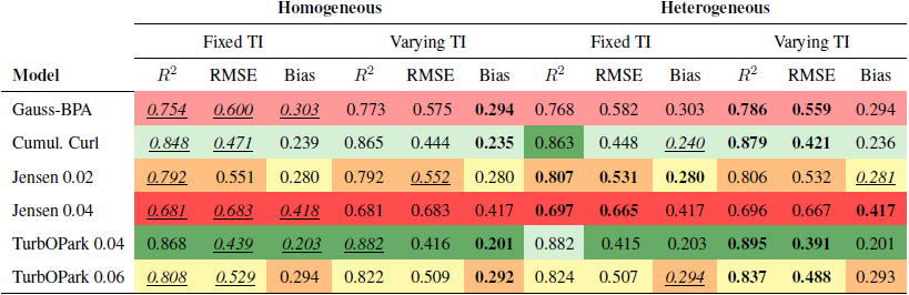
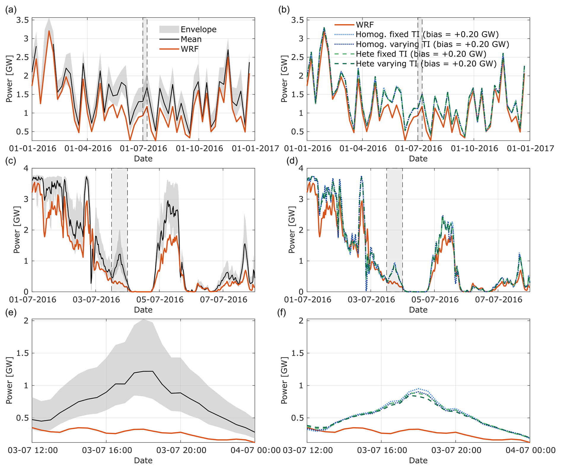
Figure D1 Total wind farm power (GW) for the BE–NL offshore wind farm cluster for simulations with PE. Shown are WRF (without PE) and the mean and envelope of all engineering models (a, c, e) and the different configurations of TurbOPark with induction factor A=0.04 (b, d, f). The top row (a, b) shows weekly averages computed from 30 min data, the middle row (c, d) shows a 1-week zoom (1–7 July 2016) at 30 min resolution, and the bottom row (e, f) shows a 12 h zoom (3 July 2016) also at 30 min resolution. The dashed box shows the time period zoom within the longer time series.

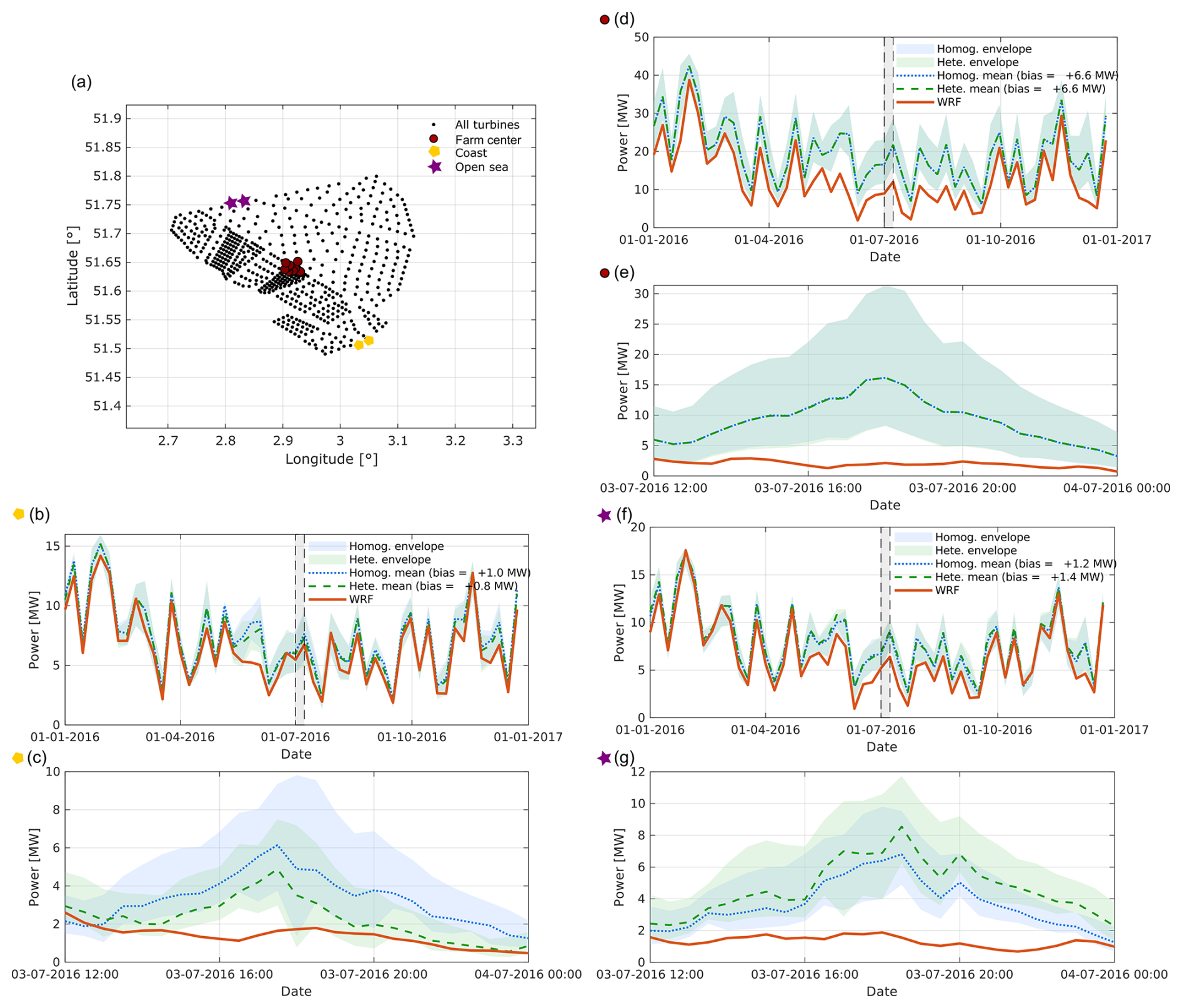
Figure D2 Grid cell power output (MW) at three representative locations within the BE–NL wind farm cluster for simulations with PE. Panel (a) shows the locations of the selected grid cells, representing the farm center as well as coastal and open-sea regions. Panels (d), (b), and (f) show weekly averages computed from 30 min data, while panels (e), (c), and (g) show a 12 h zoom on 3 July 2016 at 30 min resolution. Shown are WRF (without PE) and the mean and envelope of all engineering wake models grouped by homogeneous and heterogeneous setups. The dashed box indicates the zoomed period within the full time series. Bias is defined as the engineering wake model power minus WRF power.