Detailed experimental investigation of the aerodynamics and blade/tower interaction of a 1.5 MW wind turbine in a downwind configuration

We present a detailed experimental investigation of the flow details of the blade/tower interaction on a 1.5 MW wind turbine operated in a downwind configuration. The study aims to address claims of shortcomings in the downwind turbine concept, such as impulsive blade loading and the generation of low-frequency noise. The measurement campaign was part of a comprehensive project conducted by the National Renewable Energy Laboratory and its partners exploring the feasibility, reliability, and performance of wind turbines whose rotors are oriented downwind instead of the more traditional upwind configuration. The campaign measured blade pressure distributions at two radial positions on one blade and pressure on the tower surface at the position corresponding to the blade path of the outboard instrumented section on the blade. Pressure distributions on the blade and tower were measured using add-on pressure belts, and local inflow was measured on the blade with two five-hole probes. Despite challenging weather conditions, two measurement campaigns of different durations were successfully completed. The analysis of the datasets indicates the data are of good quality and highlights the importance of dynamically reconstructing the tower pressure measurements that used pressure belts up to 10.7 m in length. Impulse loading is found to be 100–150 N m⁻¹ on the tower and 200–500 N m⁻¹ on the blade over a time span of approximately 0.3 s. The detailed pressure measurements make the dataset well suited for use in validating high-fidelity models such as full three-dimensional computational fluid dynamics rotor simulations that include tower flow.

1 Introduction

The upwind turbine concept, in which three-bladed wind turbines are positioned with the rotor upwind of the tower, is by far the dominant industrial wind turbine configuration. This configuration has been used throughout modern wind turbine development, except in the late 1970s and early 1980s when downwind megawatt-scale prototype turbines were designed and tested in the United States and Sweden, among other places. Low-frequency noise was experienced with the MOD-1 2 MW turbine (Kelley, 1981) and other downwind turbines in the United States (Hubbard and Shepherd, 1991) as well as with the 3 MW Maglarp turbine in Sweden. Noise generation was linked to the blades passing through the wake behind the tower. The Maglarp turbine had a tubular tower, whereas the MOD-1 turbine had a lattice tower with four main poles. In addition to the low-frequency noise problem, impulsive loading of the blades during tower passage also increased fatigue loads.

These early negative experiences with downwind turbines led to the dominance of the upwind rotor concept from the late 1980s onward. However, in the last 2 decades there has been renewed interest in downwind turbines because their relative advantages over upwind turbines might increase with upscaling. In a numerical study (Bortolotti et al., 2019) comparing upwind and downwind 10 MW rotors, it was shown that the downwind rotor concept has a slightly lower cost of energy thanks to lighter blades, whose more flexible design is enabled by the relaxed constraint on blade/tower clearance. A further advantage of downwind turbines is the direction of tilt, which can have a positive impact on the power capture for hilly sites characterized by upflow conditions as well as for floating turbines (Bortolotti et al., 2019). In addition, the more flexible rotor enabled by downwind turbines can be an advantage when transporting blades by rail (Bortolotti et al., 2021).

However, potential fundamental drawbacks, like the increased low-frequency noise and impulsive loading experienced by early downwind prototypes, have only been sporadically investigated and remain unresolved. An exception is an interesting advancement in low-frequency noise modeling and simulation in which pressure fluctuations on the tower from the blade/tower interaction also seem to contribute considerably to the total low-frequency noise level (Klein et al., 2018; Zajamsek et al., 2019). In previous simulations of low-frequency noise (Viterna, 1982; Madsen et al., 2007; Madsen, 2010) only impulsive blade loading was considered to be the source of the noise.

On the experimental side on the blade/tower interaction of a down wind turbine, the Unsteady Aerodynamics Experiment conducted by the National Renewable Energy Laboratory (NREL) in 2000 should be mentioned as an old source of interesting data. This experiment was a test of an extensively instrumented model wind turbine rotor with a 10 m diameter in the giant NASA-Ames 24.4 m by 36.6 m wind tunnel. The turbine could be operated upwind and downwind of the tubular tower.

In a later study by Zahle et al. (2009), the data were used to validate a CFD model of the blade/tower interaction on the same rotor. An important observation is that in both the simulations and the measurements a strong impact on the blade response was caused by the blade passing through shed vortices from the tower. The blade/tower distance was 3.5 tower diameters in this previous experiment. In the present experiment, the blade/tower distance is only about one tower diameter, since it is an upwind turbine operated in a downwind configuration where the blade prebend reduces the blade/tower clearance. Due to this much closer distance between the blade and the tower, it is expected that the blade in the present experiment will pass through a more clean deficit as visualized in the CFD flow field simulations at a tower diameter downstream of the tower, as presented in Madsen et al. (2007). It should also be mentioned that no pressure measurements were carried out on the tower in the Unsteady Aerodynamics Experiment, preventing the full validation of the simulated blade/tower interaction.

Thus, detailed investigations of these fundamental drawbacks of downwind turbines are still needed. In 2024, a comprehensive experiment was conducted at NREL to investigate the feasibility, reliability, performance, and economic viability of wind turbines oriented downwind. In the experiment, a 1.5 MW wind turbine located at the NREL Flatirons Campus was operated in a downwind configuration. Loads, power, and acoustic emissions were monitored and compared with the upwind operation of the wind turbine. The motivation, preparation, risk mitigation, execution, and results of the full-scale downwind experiment at NREL are discussed in Bortolotti et al. (2025).

In addition to the power, loads, and acoustic measurements carried out in this experiment (Bortolotti et al., 2025), detailed measurements of the aerodynamics of the rotor and the blade/tower interaction were carried out over a shorter period within the same campaign. A novel instrumentation setup was used to measure the unsteady blade and tower surface pressure with pressure belts and to measure inflow measurements at two blade sections. Typically, aerodynamic and aeroelastic models are validated by integrated measured quantities such as loads and power derived from signals recorded by conventional instrumentation like strain gauges and accelerometers. The predictions of aerodynamic and aeroelastic codes can be satisfactorily validated in this way (Brown et al., 2024). In this case, however, the exploration of some fundamental properties of the aerodynamics of a downwind rotor and the blade/tower interaction require more detailed measurements for model validation.

The main objective of this paper is to describe the instrumentation for the detailed aerodynamic measurements with pressure belts, the deployment of the equipment, and some initial results. The organization of the paper is as follows. The turbine is presented in Sect. 2, followed by a description of the experimental setup and the deployment in Sect. 3. An overview of the measured data and some initial results from the postprocessing are presented in Sect. 4. Finally, a discussion and outlook are provided in Sect. 5 and conclusions are given in Sect. 6.

2 Turbine

The turbine adopted in this study is a 1.5 MW GE SLE machine manufactured by GE Vernova and installed at NREL's Flatirons Campus. The turbine has a rotor diameter of 77 m, hub height of 80 m, and nameplate capacity of 1.5 MW. More details about the turbine can be found in Bortolotti et al. (2025) and in older technical reports released by NREL, namely, Santos and van Dam (2015) and Mendoza et al. (2015). The turbine is highly instrumented with sensors that monitor loads and performance. Note that during the deployment of the pressure belts, an array of four microphones was also deployed in the field to record acoustic emissions in the low-frequency and audible ranges (Bortolotti et al., 2025).

2.1 Downwind rotor

The experiment consisted of flipping the rotor of the 1.5 MW wind turbine from upwind to downwind. This was achieved by pitching the blades 180° and yawing the nacelle 180°. To an observer located upwind of the turbine, the rotor continued to spin clockwise and the pitch rate of the three blades was in the same direction. However, in the downwind configuration, the blades flew behind the tower and experienced a strong wake deficit induced by the presence of the tower. The experiment was motivated by the need to quantify the increase in fatigue loads and acoustic emissions of the downwind rotors compared to the upwind rotors, since the downwind rotor configuration is proposed for very large and very flexible wind turbines (Bortolotti et al., 2025).

The downwind orientation of the rotor represents an additional challenge for the pressure belts, which were used to characterize the effect of higher-frequency step changes in loading during blade passage. Many of the findings discussed in this work also apply to conventional wind turbines with upwind rotors.

2.2 Aeroelasticity

The aeroelastic model of the turbine is available in NREL's aero-servo-elastic solver OpenFAST. The simulations presented in this study were run with OpenFAST v3.3.0 (OpenFAST, 2022), which was coupled to the industrial controller provided by GE Vernova in the form of a compiled dynamic link library. Both polars – in the form of lift, drag, and moment coefficients – and coordinates of the airfoils adopted along the span of the blades are known. The aeroelastic model uses a simple Euler–Bernoulli beam formulation for blades and towers and lifting lines for blades that include the effects of unsteady airfoil aerodynamics. Unsteady airfoil aerodynamics are simulated with the Beddoes–Leishman formulation including the Minnema–Pierce modifications (Damiani and Hayman, 2019). The tower wake is modeled with a standard Powles shadow model (Powles, 1983), which is implemented in OpenFAST as described in Moriarty and Hansen (2005).

2.3 Airfoil performance

The coordinates of the airfoils were fed to the EllipSys2D two-dimensional (2D) fluid dynamics solver (Sørensen, 1995), which generated lift and drag coefficients as a function of angle of attack for both clean and fully turbulent conditions. To capture transitional boundary layers, the e^N transition model is used (van Ingen, 1956; Drela and Giles, 1987; Michelsen, 2002). A satisfactory match was found between these predictions and the airfoil coefficients shared by GE Vernova within the aeroelastic model. These predictions were later compared with the experimental measurements (see Sect. 4).

3 Instrumentation to characterize rotor aerodynamics and blade/vortex interaction

For the detailed characterization of the aerodynamics of a blade section of the rotor blade and the flow details of the blade/tower interaction, we use a novel add-on measurement system comprising three pressure belts, two five-hole probes, and three data acquisition systems. The system was developed at the Technical University of Denmark (DTU) over the last 7 years and was recently applied in two full-scale campaigns (Madsen et al., 2022, 2025).

In the configuration for this study, we measured pressure distributions at two radial positions on one blade, each instrumented with a 32-tap pressure belt connected to two mini pressure scanners fixed to the blade surface at the trailing edge. The instrumentation included an aerodynamically shaped enclosure (referred to as a flyboard) that contained data acquisition, a WiFi system, batteries, and a five-hole probe (Fig. 1). The experimental setup measured the surface pressure along the belt, and the five-hole probe was used to reconstruct the inflow velocity. During its development, the experimental system was repeatedly tested in the Poul La Cour wind tunnel at DTU and validated against data from a conventional tap installation. The complete system for one blade section can be mounted on a full-scale wind turbine by technicians in a few hours.

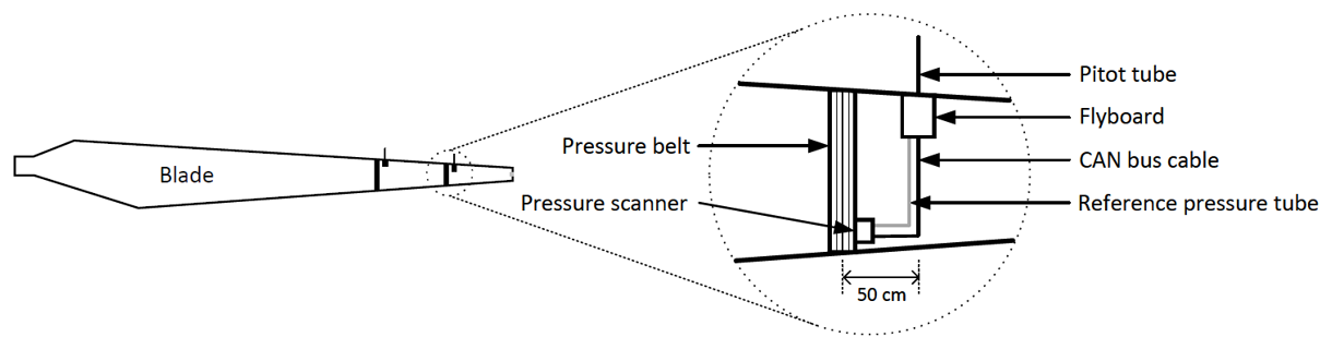
Figure 1 Schematic illustration of the inflow and pressure belt instrumentation on the 1.5 MW turbine in a downwind configuration at NREL's Flatirons Campus. See also the actual installation on the blade in Fig. 10.

In the present experiment, an additional pressure belt was installed on the tower to further characterize the blade/tower interaction by measuring the pressure fluctuations on the tower.

3.1 Belts

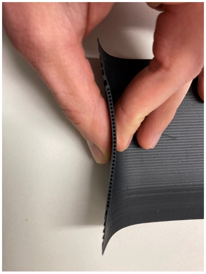
The extruded belt, with cross section shown in Fig. 2, is made of 32 channels, each with a diameter of 0.8 mm. The belt is 100 mm wide and has a maximum thickness of 1.8 mm. A pressure tap hole is drilled into each channel at a specified chord position, which is chosen to maximize the resolution of the pressure distribution and to minimize the disturbance among the pressure taps. The positioning of the taps is discussed in Sect. 3.2 and shown in the Figs. 4 and 5. Each blade belt is connected to two 16-channel miniature pressure scanners via a printed fixture. The pressure scanners, with a size of 37 mm × 32.4 mm × 9.2 mm, are operated in “calculated differential mode”, where one of the ports is used as reference and connected to the static port of the five hole probe at this radial position. The full-scale range is −400 to 200 mbar with a resolution of 0.03 mbar. The scanners are attached to the blade surface close to the trailing edge and connected with a signal cable to the data acquisition system in the flyboard. Further details of the instrumentation can be found in Madsen et al. (2022).

Figure 2 Cross section of the extruded pressure belt. Photo credit: Per Hansen, DTU.

The two blade belts were designed to be installed at distances from the blade root of 18.90 and 31.45 m, where $r/R$ = 0.51 and 0.84, the chord 1.91 and 0.96 m, and the relative thickness 25 % and 18 %. The two locations respectively correspond to 18.35 and 5.80 m from blade tip. The locations, at mid-span and toward the tip of the blade, were chosen to focus on a simpler case where flow is assumed to be close to 2D. Future experiments will be able to focus on more challenging blade regions, such as closer to the root and tip, where flow is known to be more three-dimensional (3D) (Bangga, 2018; Jeong and Ha, 2021). At the two locations, the chords are known and the airfoils correspond to two master airfoils of known coordinates and performance. The length of each belt was set to ensure that the ends of the belt reached the trailing edge on both the suction and pressure sides.

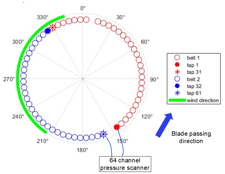
Figure 3 Orientation, tap layout, and connection to pressure scanner for the two tower belts.

The belts on the tower were installed at a height of 46.7 m from the base of the tower. The height was chosen because it corresponds to the tower path of the outer belt on the blade in an undeflected turbine configuration. To cover the entire circumference of the tower, two belts were wrapped around the tower, each made of two 32 channel segments of a length of 9.7 m. The two segments were vertically shifted by one belt width (see the photo on the right in Fig. 10) to allow the connection of a 64-channel pressure scanner, which was installed in an almost airtight box attached to the tower opposite the prevailing wind direction at a location approximately 1 m above the pressure belts. The scanner is the Scannivalve MPS4264 electronic pressure scanning module with a full range of 4 inH2O (0.145 Psi) and with the static port open inside the box with the scanner. Unlike the belts on the blades, the positions of the taps on the tower were uniformly distributed, except for a few faulty taps not shown (Fig. 3).

3.2 Tap layout of blade pressure belts

The pressure tap (also known as port or orifice) layout used at both belt locations was based on a cosine spacing law. This arrangement produced higher port density at the leading edge and sparser port density at the trailing edge of both pressure and suction surfaces. The spanwise spacing of ports minimized upstream ports tripping the boundary layer for downstream ports, though some degree of disruption of the airfoil boundary layer might be expected in some conditions from the spanwise-running ramps at the edges of the pressure belt (cf. Brown et al., 2018). The port layout is shown in Figs. 4 and 5. Both the (a) chord positions (Figs. 4a and 5a) and (b) span positions (Figs. 4b and 5b) of the ports are presented. The span position plots show the pressure belt from above as wrapped around the leading edge at s_arc≈ 2 m and s_arc≈ 1 m for the two stations.

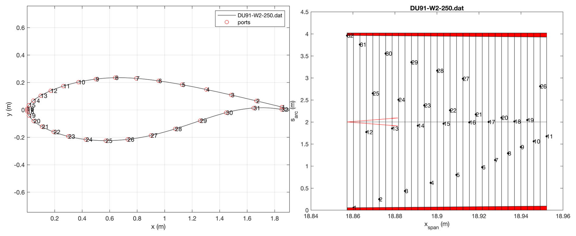
Figure 4 Pressure tap layout for inboard station showing (a) chord-wise positions and (b) spanwise positions.

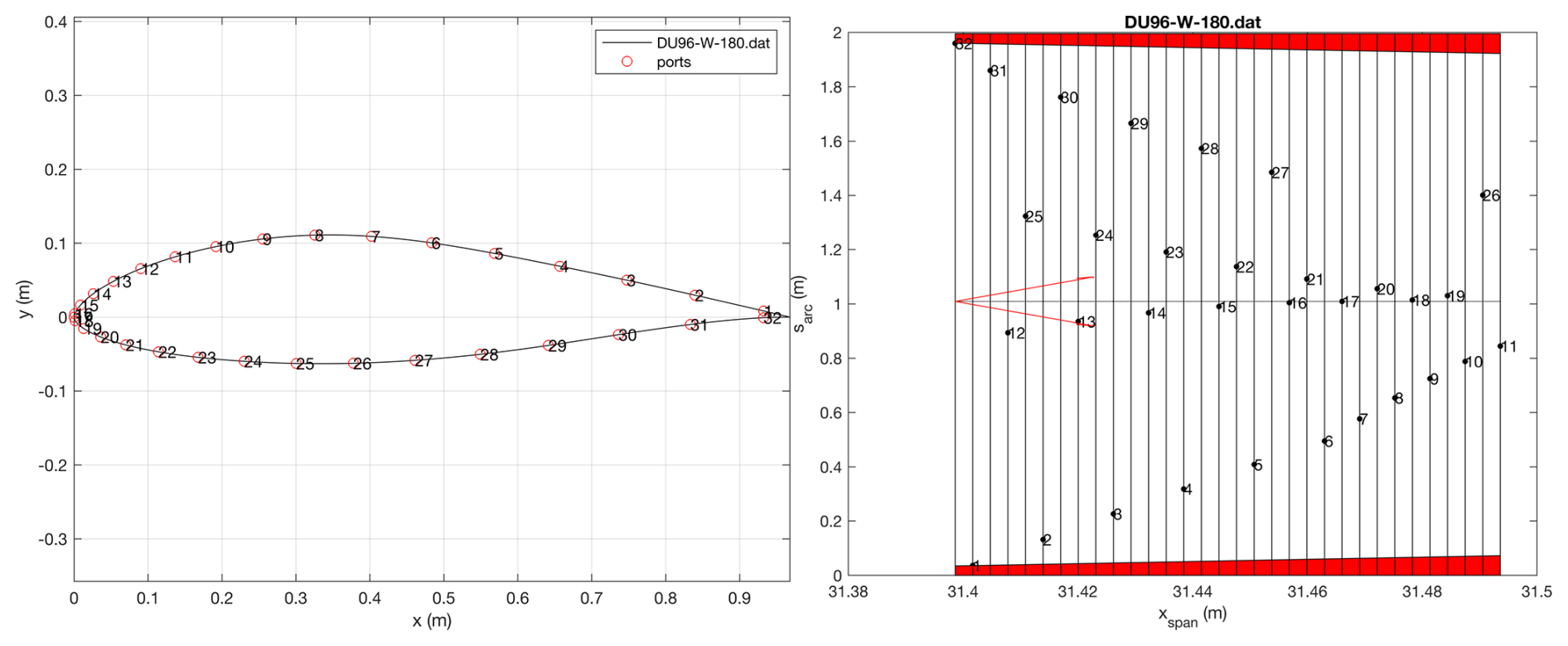
Figure 5 Pressure tap layout for outboard station showing (a) chord-wise positions and (b) spanwise positions.

Note the spanwise layout axes are not to scale. The red vectors are 15° wedge angles from vertical to assess downstream transition spreading. Additionally, pressure belt tubing connectors interfered with optimal port locations near the trailing edge. These interference areas are depicted as shaded red trapezoids in Figs. 4b and 5b.

In Fritz et al. (2024) the authors initially developed an optimization routine to minimize the number of pressure ports needed to accurately measure lift coefficient. This work showed that 32 pressure ports with cosine spacing already had a lift coefficient error below 0.01. Therefore, there was not a significant advantage to using an optimized layout.

3.3 Dynamic calibration of the pressure belts

Due to the long blade sections and large tower diameter of the 1.5 MW turbine, the pneumatic pressure belts used in this experiment included extended runs of small-diameter embedded tubing that connected surface taps to miniature pressure scanners. Such configurations are known to introduce dynamic distortions in unsteady pressure measurements, including signal attenuation, resonance amplification, and phase delays. These distortions result from viscous friction and acoustic wave propagation within the tubing and are a function of frequency (Bergh and Tijdeman, 1965). To ensure accurate pressure signals (both in magnitude and time), which are necessary for analyzing unsteady aerodynamic phenomena such as blade/tower interaction, it was essential to characterize and compensate for each port's dynamic response.

Following the full-scale measurement campaign, the pressure belts were removed from the turbine and transferred to a laboratory environment for post-test characterization of the channel connecting the taps to the transducers. Each pressure channel was individually characterized using an in situ tubing characterization device, which generated a rapid pressure pulse at the belt inlet (e.g., the surface pressure). The resulting pressure response at the scanner end of the tubing (e.g., the remote-raw pressure) was recorded simultaneously with the surface pressure, thereby enabling quantification of the system's frequency-domain transfer function. The tubing system geometry was then modeled, and theoretical transfer functions (e.g., the system response) were generated and compared with experimental data to accurately capture variations in the as-built geometry (Mears et al., 2024). In practice, reconstruction of the surface pressure requires an inverse process; the remote-raw pressure is used to estimate the surface pressure. A Wiener-filtered inverse model of the system response was developed based on the as-built tubing system geometry and compared with each port's measured reference data, following the methodology of Nikoueeyan and Naughton (2024). The filtering is necessary to avoid amplifying noise present in the remote-raw pressure when reconstructing the surface pressure. These models facilitated the derivation of optimal reconstruction filters capable of suppressing noise amplification while accurately restoring phase and amplitude across the relevant frequency range.

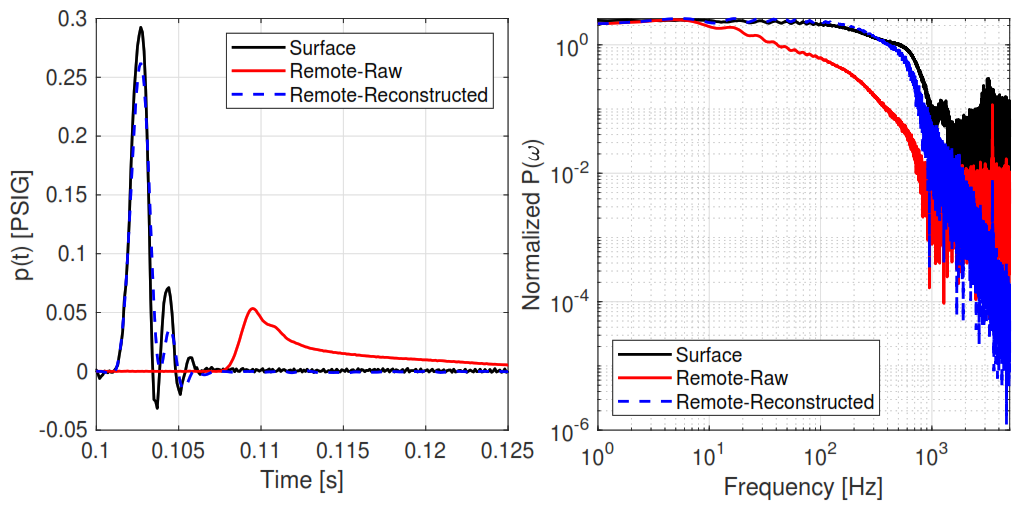
Figure 6 Dynamic calibration of the pressure channels. Left: response of one of the pressure channels to a pressure pulse applied at the surface. Both the raw measured signal at the scanner and the reconstructed pressure are shown. Right: the same three signals in the frequency domain.

Figure 6 presents an example of the dynamic characterization of one representative pressure port. The left panel shows the recorded pressure signals in the time domain, clearly illustrating the distortions induced by the tubing system. The surface pressure exhibits a sharp high-frequency pressure pulse, whereas the remote-raw pressure is significantly delayed and attenuated, showing resonant behavior (overshoot) caused by acoustic and frictional effects within the tubing. The Wiener-filtered reconstruction produces the remote-reconstructed pressure that demonstrates a significantly improved comparison to the surface reference input, effectively correcting both amplitude attenuation and phase delay. The frequency-domain plot (right panel) confirms these observations: the pressure pulse applied to the surface has frequency content from low frequency out past 500 Hz, the remote-raw pressure is significantly attenuated at all frequencies greater than 10 Hz, and the remote-reconstructed pressure accurately restores the broadband frequency content up to 400 Hz. The ability to reconstruct pressure signals with frequency content up to 400 Hz ensures the ability to resolve unsteady aerodynamic phenomena relevant to blade/tower interactions.

It is important to note that the tubing characterization step was conducted at a significantly higher sampling frequency than that used during field testing to ensure increased fidelity of the modeling approach. However, the actual field measurements were acquired at a sampling frequency limited to 100 Hz; consequently, the maximum reconstruction frequency of the test data will be constrained by this sampling frequency bandwidth.

The reconstructed pressure signals were compared against the known input signals from the calibration procedure in both time and frequency domains. For each port, the reconstruction was evaluated based on its ability to recover the sharp pressure rise and broadband content of the calibration impulse. Overall, the reconstruction technique demonstrated effective recovery of high-frequency pressure content up to approximately 20 Hz across many channels, which is critical for resolving unsteady aerodynamic features in the current field test campaign.

The validated reconstruction models were then applied to the raw pressure data acquired during the two downwind test campaigns. The reconstruction was performed as a postprocessing step, channel by channel, using the individualized Wiener-filtered system response model developed for each port. The corrected pressure signals provide a better representation of the unsteady surface pressures on the blade and tower, with significantly reduced influence from tubing-induced distortions through the reconstruction process. These reconstructed datasets form the basis for the aerodynamic analysis and comparisons with numerical predictions discussed in subsequent sections.

3.4 Flyboard, data acquisition, and five-hole probe

The flyboards, one adjacent to each belt on the blade, consist of a metal frame with a plastic cover that aims to minimize impact on the surrounding airflow. The dimension of the flyboards is approximately 30 cm in spanwise and chordwise directions and about 10 cm in height; see Fig. 10. They contain the data acquisition unit, WiFi, and batteries (see the middle photo in Fig. 10). Each flyboard also carries the five-hole probe, which has a length of 0.42 m. The data acquisition system samples the data from the pressure scanners on the blade, the five-hole probe, and a three-axis accelerometer in the flyboard at a rate of 100 Hz; the data are GPS time-stamped. The WiFi antenna transmits data in real time to the ground for visualization and postprocessing. Note that if the WiFi malfunctions, the data are also stored in the data acquisition system housed on the flyboard and can be retrieved physically by accessing the flyboard. To maximize battery charge, the data acquisition and WiFi system has a start/stop function that can be controlled remotely, so the system only operates when measurements are ongoing.

A third data acquisition system is installed at the bottom of the tower and samples the 64 channels from the pressure scanner connected to the pressure belts on the tower at 100 Hz. In postprocessing the data are aligned with the blade pressure data based on the GPS timestamp.

3.5 Calibration of the five-hole probes and data processing

The five-hole probes, manufactured by Aeroprobe Inc., have a diameter of 6.35 mm and a spherical head. The pressure ports and the probe coordinate system are shown in Fig. 7. Two different probe coordinate systems were used in this investigation. The coordinate system defined by the angle of attack α and the angle of side slip β was used to characterize the aerodynamics at the wind turbine blade. The coordinate system defined by the yaw angle θ and the roll angle Φ exploits the symmetry of the theoretical shape of the five-hole probe. The conversion between the two coordinate systems is given by

$$\begin{array}{}\text{(1)}& {\displaystyle }& {\displaystyle }\mathit{\alpha }=\arctan \left(\sin \right(\mathit{\varphi }\left)\tan \right(\mathit{\theta }\left)\right),\text{(2)}& {\displaystyle }& {\displaystyle }\mathit{\beta }=\arcsin \left(\cos \right(\mathit{\varphi }\left)\sin \right(\mathit{\theta }\left)\right),\end{array}$$

and

$$\begin{array}{}\text{(3)}& {\displaystyle }& {\displaystyle }\mathit{\varphi }=\arctan \left(\sin \right(\mathit{\alpha })/\tan (\mathit{\beta }\left)\right),\text{(4)}& {\displaystyle }& {\displaystyle }\mathit{\theta }=\arccos \left(\cos \right(\mathit{\alpha }\left)\cos \right(\mathit{\beta }\left)\right).\end{array}$$

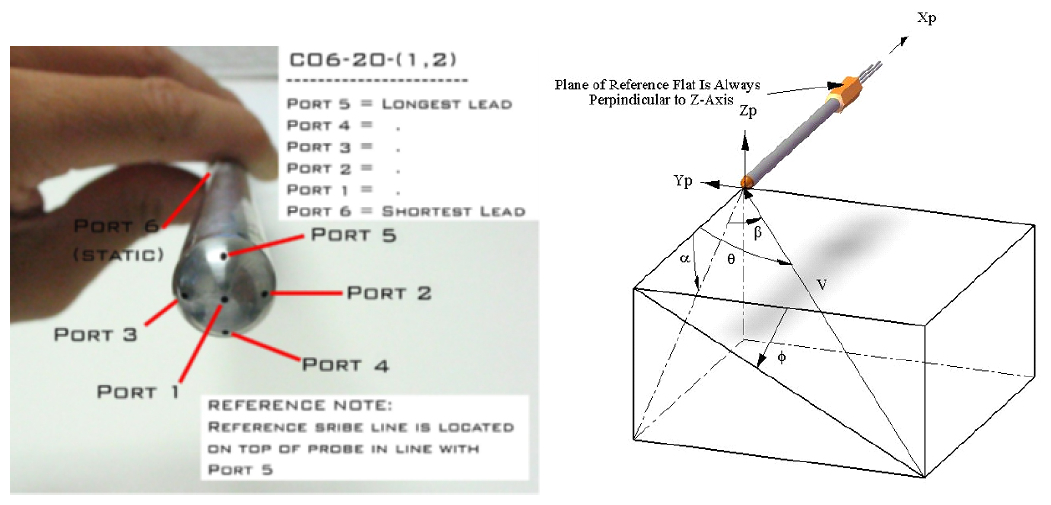
Figure 7 Left: a photo of the pressure ports of the five-hole probe from the Aeroprobe manual. Right: the probe coordinate system.

Figure 8 The calibration setup for the five-hole probe.

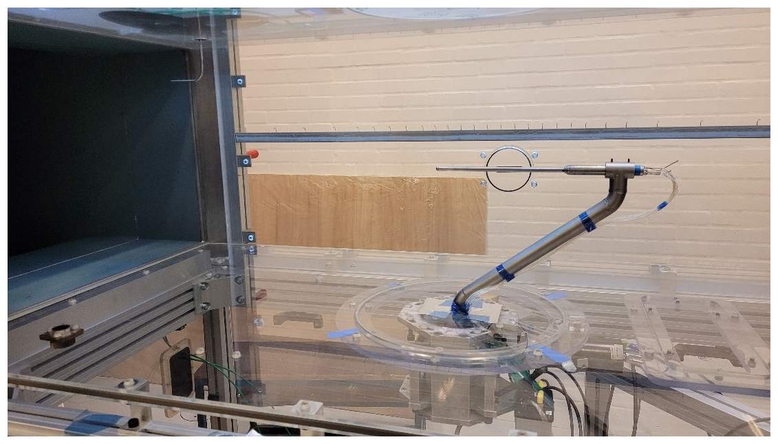
The five-hole probe was calibrated in the red wind tunnel at DTU (Ildvedsen, 2017). The red wind tunnel provides a maximum flow velocity of 40 m s⁻¹ and a turbulence intensity of less than 0.1 %. The test section is 2000 mm long and has a cross section of 750 mm × 500 mm. The tip of the five-hole probe was placed on a turn table 750 mm downstream of the inlet (Fig. 8). A reference Pitot tube was placed 60 mm downstream of the inlet.

The calibration was performed at two flow speeds, 20 and 40 m s⁻¹. Five differential pressures were measured during calibration:

$$\begin{array}{}\text{(5)}& {\displaystyle }\mathrm{\Delta }{p}_{\mathrm{16}}& {\displaystyle }=p_{\mathrm{1}}-p_{\mathrm{6}},\text{(6)}& {\displaystyle }\mathrm{\Delta }{p}_{\mathrm{23}}& {\displaystyle }=p_{\mathrm{2}}-p_{\mathrm{3}},\text{(7)}& {\displaystyle }\mathrm{\Delta }{p}_{\mathrm{45}}& {\displaystyle }=p_{\mathrm{4}}-p_{\mathrm{5}},\text{(8)}& {\displaystyle }\mathrm{\Delta }{p}_{t\mathrm{6}}& {\displaystyle }=p_{\mathrm{t}}-p_{\mathrm{6}},\text{(9)}& {\displaystyle }\mathrm{\Delta }{p}_{\mathrm{s}\mathrm{6}}& {\displaystyle }=p_{\mathrm{s}}-p_{\mathrm{6}},\end{array}$$

where p_n is the pressure at port n=1…6, p_t is the total pressure from the reference Pitot tube, and p_s is the static pressure from the reference Pitot tube. The reference dynamic pressure is calculated by

$$\begin{array}{}\text{(10)}& q=\mathrm{\Delta }{p}_{\mathrm{t}\mathrm{6}}-\mathrm{\Delta }{p}_{\mathrm{s}\mathrm{6}}.\end{array}$$

The four coefficients,

$$\begin{array}{}\text{(11)}& {\displaystyle }{C}_{\mathit{\alpha }}& {\displaystyle }={\displaystyle \frac{\mathrm{\Delta }{p}_{\mathrm{45}}}{\mathrm{\Delta }{p}_{\mathrm{16}}}},\text{(12)}& {\displaystyle }{C}_{\mathit{\beta }}& {\displaystyle }={\displaystyle \frac{\mathrm{\Delta }{p}_{\mathrm{23}}}{\mathrm{\Delta }{p}_{\mathrm{16}}}},\text{(13)}& {\displaystyle }{C}_{\mathrm{q}}& {\displaystyle }={\displaystyle \frac{\mathrm{\Delta }{p}_{\mathrm{16}}}{q}},\text{(14)}& {\displaystyle }{C}_{\mathrm{s}}& {\displaystyle }={\displaystyle \frac{\mathrm{\Delta }{p}_{\mathrm{s}\mathrm{6}}}{q}},\end{array}$$

are calculated by using the calibration pressures from the reference Pitot tube. The coefficients C_α and C_β are solely defined based on pressures measured with the five-hole probe. They are used to infer the angle of attack and angle of side slip according to the procedure outlined below. The static and dynamic pressure of the flow can only be inferred directly from the measured pressures at the five-hole probe if it is aligned with the flow. The coefficients C_q and C_s were introduced to compensate for the effects of probe misalignment by calibration when determining the static and dynamic pressure.

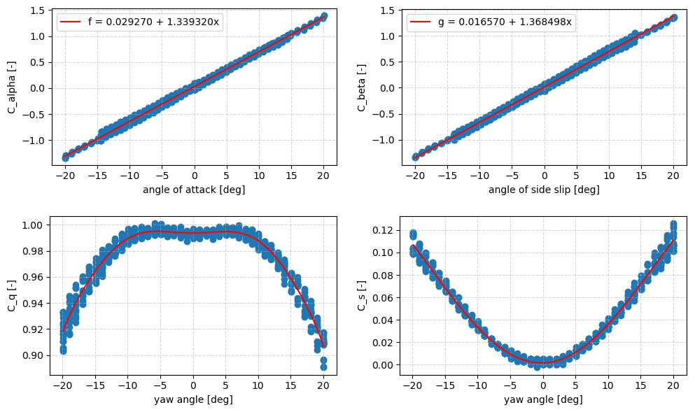
Figure 9 The calibration coefficients of the five-hole probe. The scatter of the calibration samples is due to a variation in the complementary angle in the respective coordinate system.

The results for a flow speed of 20 m s⁻¹ are displayed in Fig. 9. The results of the calibration at a flow speed of 40 m s⁻¹ are not displayed, because the result is very similar to the result at 20 m s⁻¹. In addition, it was found that each calibration coefficient depended mainly on one flow angle and the influence of the other flow angle could be neglected. Hence, the approximations

$$\begin{array}{}\text{(15)}& {\displaystyle }{C}_{\mathit{\alpha }}& {\displaystyle }=f\left(\mathit{\alpha }\right),\text{(16)}& {\displaystyle }{C}_{\mathit{\beta }}& {\displaystyle }=g\left(\mathit{\beta }\right),\text{(17)}& {\displaystyle }{C}_{\mathrm{q}}& {\displaystyle }=h\left(\mathit{\theta }\right),\text{(18)}& {\displaystyle }{C}_{\mathrm{s}}& {\displaystyle }=k\left(\mathit{\theta }\right),\end{array}$$

were made. The calibration coefficients do not depend on flow speed. This approximation holds if the flow Mach number is lower than 0.3. The calibration functions were assumed to have polynomial shapes and were displayed in red in Fig. 9.

The data reduction using the calibration coefficients was done in the following way.

• C_α and C_β were computed with the measured five-hole probe pressure differentials.

• The functions f and g were inverted to get α and β.

• θ was computed from α and β.

• C_q and C_s were computed from θ with h and k.

• The dynamic pressure was computed as q=C_qΔp₁₆.

• The pressure coefficients at the belt ports were computed as $c_{\mathrm{p},\mathrm{b}}=\frac{p_{\mathrm{b}}-p_{\mathrm{6}}}{q}-C_{\mathrm{s}}$, where p_b are the pressures at the ports of the belt.

3.6 Deployment

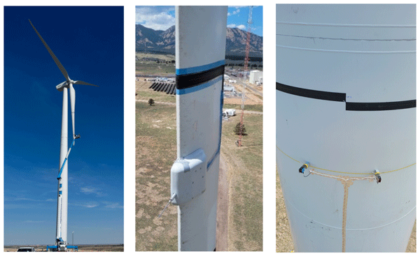
The deployment of the measurement system, which was planned for the last 2 weeks in April 2024, was challenged by rainy, windy, and cold weather. On Sunday, 21 April, the weather was dry and sunny, but the low temperature in the morning required the removal of ice from the top of the nacelle, the hub, and the blade surface in the area for the belt before the installation could start. Despite nonoptimal installation conditions, both pressure belt systems on blade 1 were installed on this day from a lift (left and middle photos in Fig. 10). The already installed inner belt and flyboard are visible at the mid-span of blade 1.

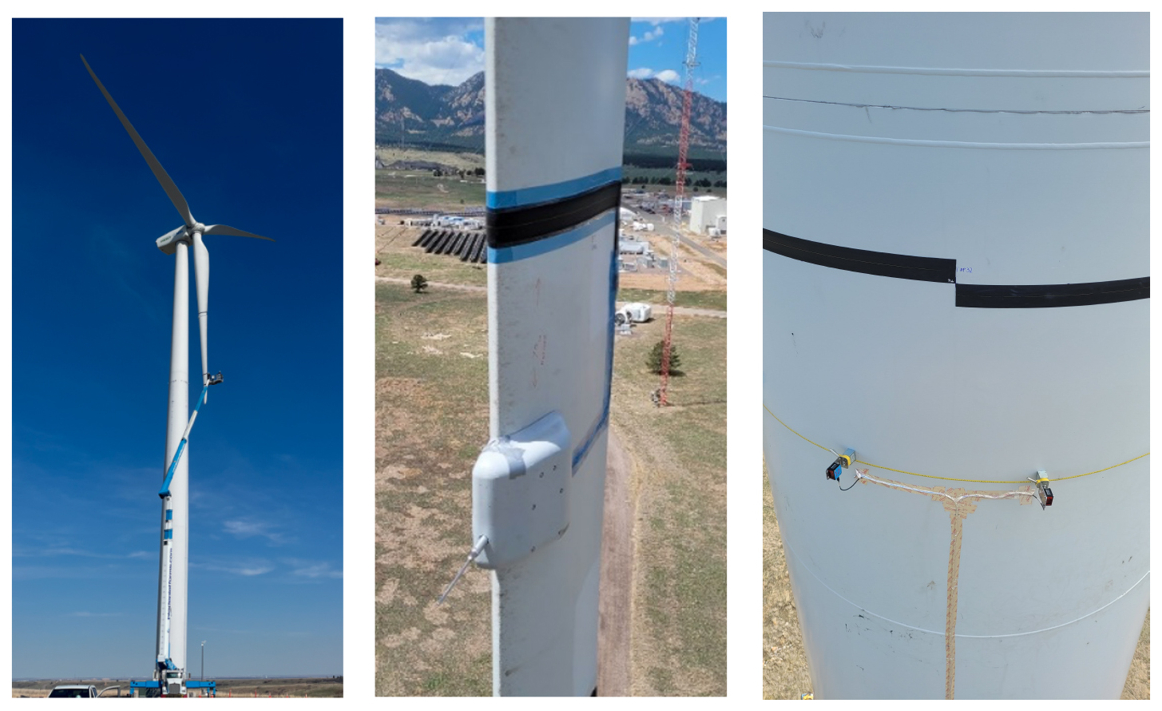
Figure 10 Left: installation of the outer belt on blade 1 of the GE 1.5 MW wind turbine. The rotor is parked in a downwind configuration. The inner belt and flyboard are visible at the mid-span of blade 1. The belt on the tower had not yet been installed when this photo was taken. Photo credit: Pietro Bortolotti, NREL. Middle: close-up view of the flyboard, five-hole probe, and belt installed at the outer blade location. Photo credit: Per Hansen, DTU. Right: the belts on the tower, each covering half of the circumference, were installed 1 m above the laser sensors and at the height of the outer belt on blade 1. Photo credit: Per Hansen, DTU.

The middle photo of Fig. 10 shows the belt and the flyboard installed at the outer blade span location. The belt is toward the blade root, and the flyboard is toward the blade tip. The installation included the correct positioning of the two five-hole probes, which were aligned with the mean angle of attack at the two spanwise stations. Angles of attack for alignment of the five-hole probes were estimated by running the turbine model in OpenFAST through six turbulent seeds from the normal turbulence model with an average wind speed at the hub height between 5 and 11 m s⁻¹ in steps of 1 m s⁻¹.

The installation of the measurement system without the tower belt was completed in the morning of the following day. Instead of taking time to mount the tower belt, a measurement campaign of several hours was conducted that day.

Unfortunately, rainy weather followed the next several days, until Monday, 29 April, when it was possible to install the tower belt. The right photo of Fig. 10 shows the installed pressure belt with the vertical displacement of the belts relative to each other. A short measurement campaign was conducted in the afternoon that day with all three pressure belts working.

4 Results

4.1 Overview of collected data

Data were collected on two days: 22 April (D1) and 29 April (D2) 2024. During D1, only the two blade systems were available. During D2, all systems were available, but data on the inner station of the blade were partly corrupted by the presence of water in the inner blade belt.

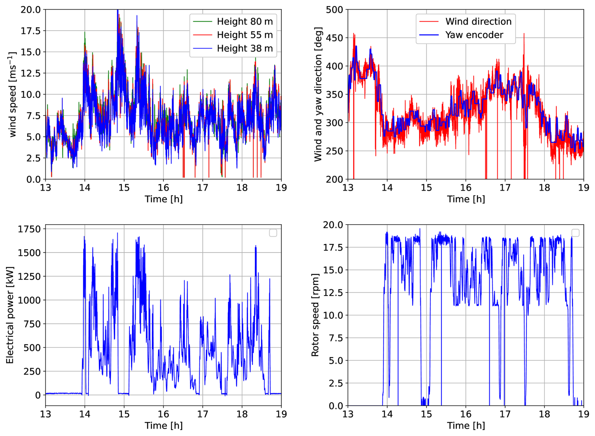
Figure 11 Upper-left: wind speed at three different heights during the D1 measurement campaign. Upper-right: wind direction at 38 m height in the meteorology mast compared to the yaw encoder sensor. Lower-left: wind turbine electrical power. Lower-right: rotor rotational speed.

4.1.1 Campaign 1 on 22 April 2024

An overview of wind conditions during the D1 campaign is shown in Fig. 11 together with the turbine electrical power and rotor speed. As seen by the measured wind speeds at three heights in Fig. 11 (upper-left), the wind varied a lot during the first 2–3 h of the measurement campaign. Later in the afternoon, the wind speed was more stable. The large variations in wind speed had a positive impact: during this short campaign of about 5 h, the turbine operated from the cut-in wind speed to the rated power as seen in the graphs of wind speed (upper-left graph) and electrical power (lower-left graph) of Fig. 11 and with considerable rotor speed variations, as shown in the lower-right graph. The drawback is the large variations in wind direction as shown in the upper-right graph, which result in high instantaneous yaw errors, which limit useful data when a narrow filter on the yaw error is applied.

4.1.2 Campaign 2 on 29 April 2024

On the morning of 29 April, the measurement system was prepared for a new measurement campaign after almost 1 week of rain. The preparation comprising the mounting of the tower pressure belt system lasted until around 15:00 local time, and, as the decommissioning of the system was prepared for late afternoon, only about 1 h of measurement was possible. However, 1 h of high-quality data were acquired from the outboard blade pressure belt and the tower belt, enabling detailed investigation of the blade/tower interaction. Together with the previously acquired dataset of about 5 h, the main objectives of the experiment and the instrumentation were fulfilled. In addition, it demonstrated the importance of accurately resolving the time dependence of both the blade and the tower pressure distributions.

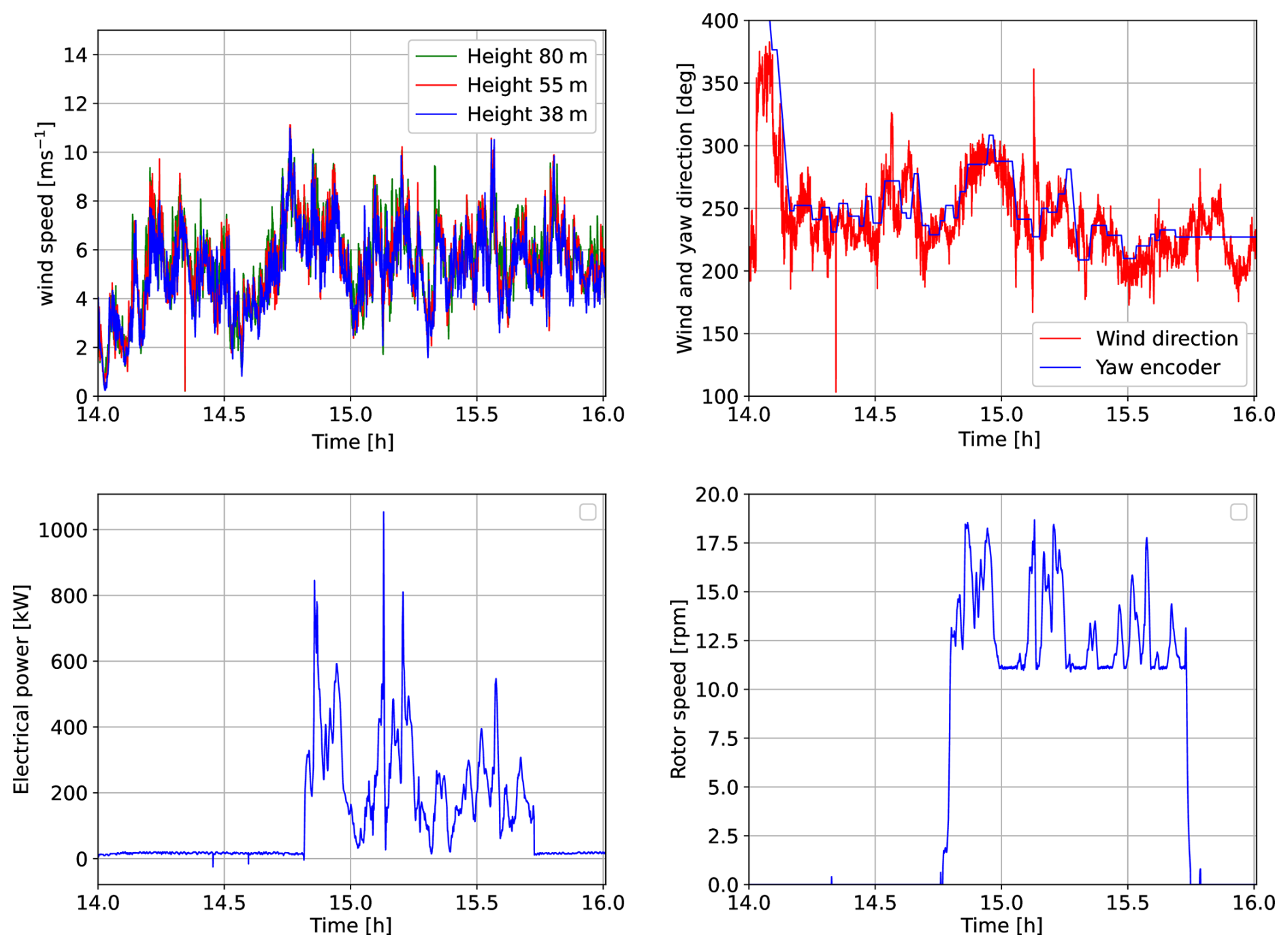
Figure 12 Upper-left: wind speed at three different heights during the D2 measurement campaign. Upper-right: wind direction at 38 m height in the meteorology mast compared to the yaw encoder sensor. Lower-left: wind turbine electrical power. Lower-right: rotor rotational speed.

An overview of the wind conditions during the D2 campaign is shown in Fig. 12 together with graphs of electrical power and rotor speed. In contrast to the wind conditions of D1, the wind speed was much more stable during the afternoon of D2, and instantaneous changes in the wind direction were also smaller (Fig. 12).

During the interval measured on D2, the turbine operated below rated power, as seen in the lower-left graph of Fig. 12, but most of the time it was well above zero power. In addition, the rotor speed varied from the minimum setting to almost maximum speed, making the data set a good representation for general turbine operation.

4.2 Data processing

The pressure data were filtered using conditions extracted from the SCADA data to find time periods of fully operational data. The following filters were applied:

• active power larger than 150 kW,

• blade pitch angle smaller than 15°,

• absolute value of the yaw error smaller than 10°.

The application of these filters reduced the dataset to 1.4 h for D1 and 0.28 h for D2.

Data from the five-hole probe were first converted to inflow velocity and inflow angle using the calibration obtained during wind tunnel testing. Next, these quantities were used to estimate the angle of attack and relative velocity based on EllipSys2D computational fluid dynamics (CFD) simulations. The trailing edge pressure measured from the belts was interpolated first, and then the pressures were integrated to determine aerodynamic forces and coefficients. The results were time-averaged (10 samples, resolving up to 10 Hz), filtered based on SCADA data, and binned in terms of angle of attack and azimuth. The pressure coefficient, C_p, for the measured data was calculated using the static and dynamic pressure from the five-hole probe.

4.3 Pressure coefficient

In Fig. 13, the measured C_p distribution of the inboard section binned on various angles of attack is presented and compared to EllipSys2D CFD results. There is a clear discrepancy, especially on the suction side, resulting in an overall loading difference with the model results. This could be attributed to shape and roughness imperfections but is probably not least due to the impact of three dimensional flow effects in combination with a rather thick airfoil of 25 % in atmospheric turbulent flow. The missing suction peak could be due to this.

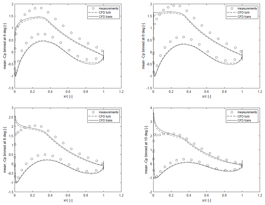
Figure 13 Pressure coefficients at (upper-left) 4, (upper-right) 6, (lower-left) 8, and (lower-right) 10° for the inboard blade station. Experimental mean values are reported with circles, and the lines are the results from EllipSys2D with fully turbulent (dashed) and free transition (solid) conditions.

However, the conversion of the measured inflow angle by the five hole probe to AoA based on 2D CFD simulations is also an important source of uncertainty combined with the uncertainty in estimating the geometrical angle of the five hole probe relative to the local chord.

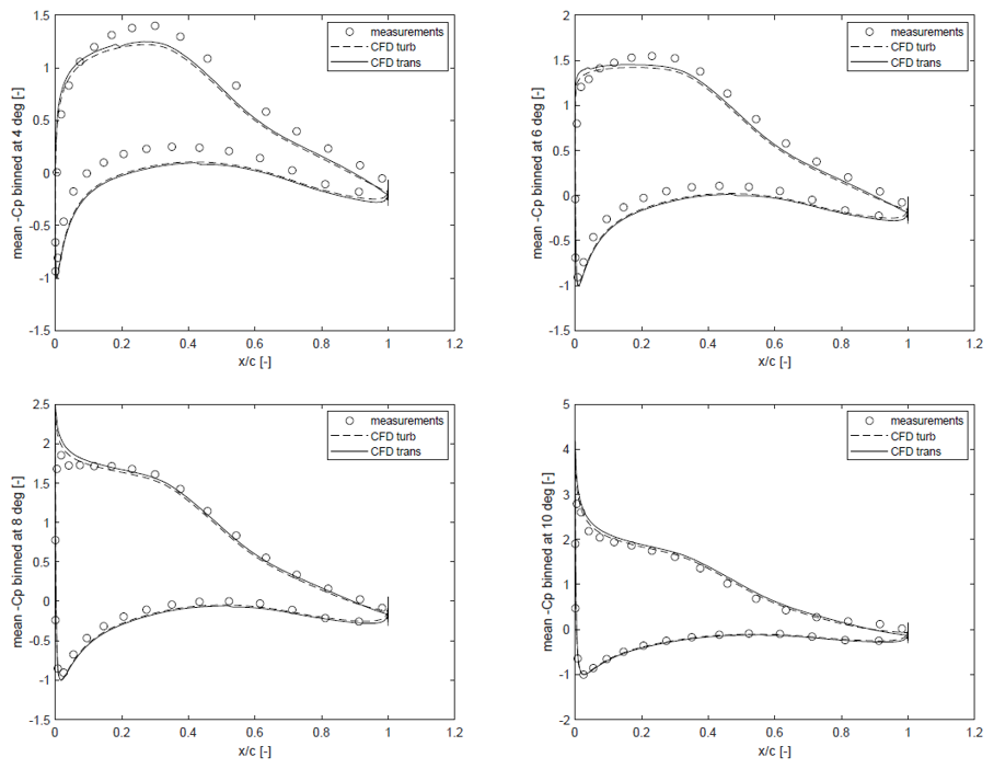
Figure 14 Pressure coefficients at (upper-left) 4, (upper-right) 6, (lower-left) 8, and (lower-right) 10° for the outboard blade station. Experimental mean values are reported with circles, and the lines are generated by EllipSys2D with fully turbulent (dashed) and free transition (solid) conditions.

In Fig. 14, the measured C_p distribution of the outboard section binned on various angles of attack is presented and compared to EllipSys2D CFD results. The simulation results show a good match with the measurements, especially the fully turbulent ones, indicating good estimation of the overall loading. The improved correlation between measurements and simulations for this station compared with the inboard station mentioned above can probably also be attributed to a more 2D inflow at this station. We also notice here that the suction peak at 8° and, in particular, at 10° is well captured by the pressure measurements.

4.4 Lift coefficient

In Fig. 15, the measured binned lift coefficients of both sections are compared to the EllipSys2D CFD data. The measurements for the inboard section indicate a lower lift slope, which could be attributed to shape and roughness imperfections and the uncertainty mentioned in the conversion method from the input angle to the angle of attack, the former being visible in the pressure distributions. The deviations correspond to the pressure distribution differences shown in Fig. 13.

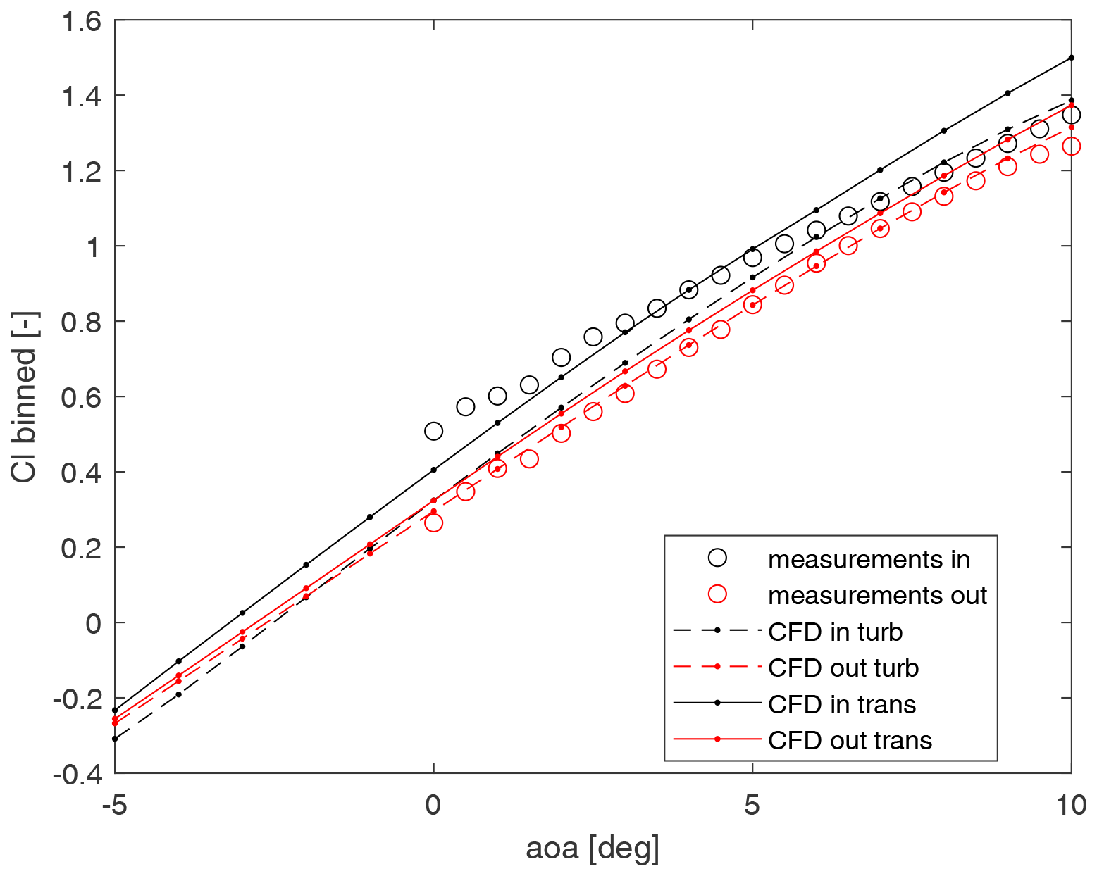
Figure 15 Binned lift coefficient as a function of angle of attack. Experimental mean values are reported with circles, and the lines are generated by EllipSys2D with fully turbulent (dashed) and free transition (solid) conditions (in: inboard, out: outboard)).

The measurements for the outboard section match quite well with the fully turbulent simulation data, which is also in line with the good correlation between the experimental and simulated pressure distributions in Fig. 13.

4.5 Blade/tower interaction

4.5.1 Measured blade and tower sectional aerodynamic loads

The integrated total aerodynamic loads F tower and F_n blade from the measured pressure distributions on the tower and the outboard blade section for a period of about 0.5 h of the second measurement campaign is shown in Fig. 16, followed by Fig. 17 showing the wind speed and electrical power during the same time sequence. There is overall good correlation between the variations in blade and tower loads, but the level of the tower loads is 3 to 5 times lower due to the difference between the speed of the free wind forcing the tower and the relative velocity determining the sectional force of the blade.

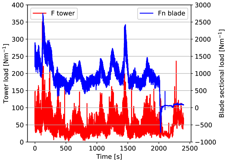
Figure 16 Time traces of the total aerodynamic load on the tower and the outboard normal sectional aerodynamic load during the second campaign.

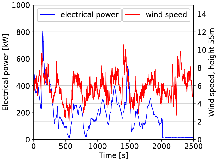
Figure 17 Time traces of wind speed and electrical power during the same period as the blade and tower loads shown in Fig. 16.

In Figs. 18 and 19, we zoom in on a time span of only 10 s to explore the details of the impulsive loading. In Fig. 18 the wind speed is relatively low, and we can see that the tower force increases from a low mean level when the blade passes and with an impulsive force typically around 100 N m⁻¹. The impulsive force of the blade is a decrease in the load level of 200–400 N m⁻¹. At a higher wind speed, as is the case in Fig. 19, the tower force decreases from the mean level with an impulsive amplitude of 100–150 N m⁻¹ compared to the impulsive blade force of 200–500 N m⁻¹. The difference in this impulsive load pattern on the tower from low to high wind speed is a subject of further investigation.

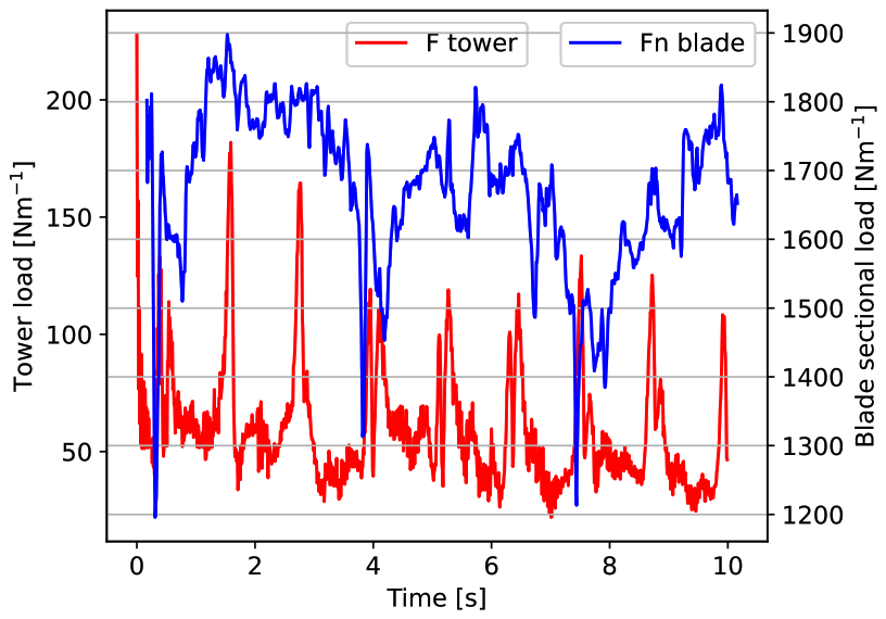
Figure 18 A close-up of time traces at low wind speed of the aerodynamic load on the tower and the outboard sectional aerodynamic blade load.

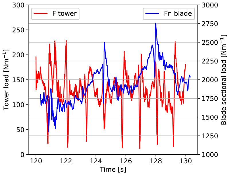
Figure 19 A close-up of time traces at high wind speed of the aerodynamic load on the tower and the outboard sectional aerodynamic blade load.

4.5.2 Details of the pressure variation on the tower

Next, we look at the details of the pressure variation on the tower. The time traces of the measured pressure at two ports are shown in Fig. 20, together with the reconstructed pressure signals (dashed lines). Port 32 is in the compass direction of about 325° and thus upstream of the tower and the rotor and on the windward side of the tower (Fig. 3). The port is at the end of pressure belt 2 and has the longest tube length of about 10.7 m (length of the connection tube to the scanner ≈ 1 m plus half the circumference of the tower, 9.7 m. This gives a strong impact of the dynamic reconstruction as evidenced by comparing the solid (raw) and reconstructed (dashed blue) lines in Fig. 20). The pressure drop in the reconstructed signal is much deeper and the time delay of the raw signal is removed. On the other hand, the reconstruction is not visible for port 1 at a compass angle of 145°. Port 1 has the shortest length to the scanner, with a tube length of about 1 m, as the raw and reconstructed pressure are nearly identical except near the peaks.

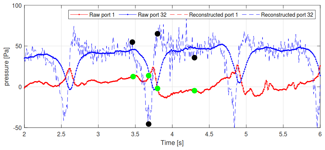
Figure 20 Time trace of tower pressure at two ports. The dots show the time at which polar plots of the pressure distribution are shown in Fig. 21.

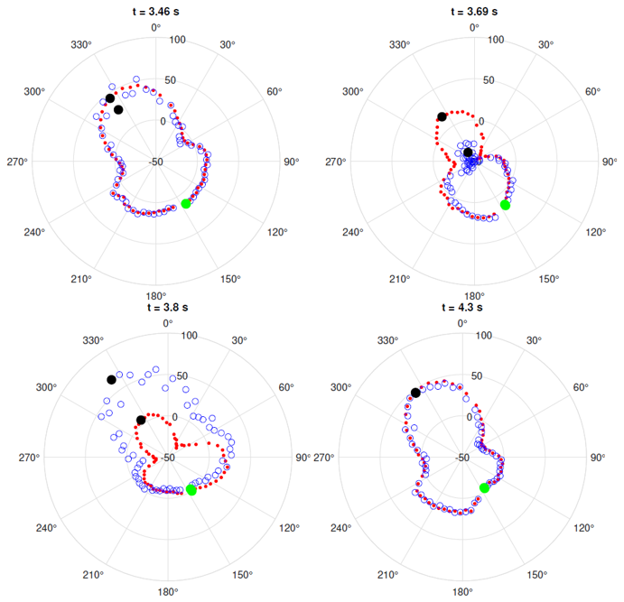
Figure 21 Tower pressure distributions at different times during blade passage. Red dots are raw pressure and blue circles are reconstructed pressure. The unit in the polar plot is Pa. The big green and black dots indicate port 1 at a compass angle of approximately 145° and port 32 at an angle of approximately 325°, respectively. See Fig. 3 for the orientation of the belt and numbering of taps. Time traces of the pressure at these two ports are shown in Fig. 20.

The strongest variation when comparing the pressure variations at ports 1 and 32 is on the upwind tower side away from the blade passage (Fig. 3). In planning the pressure tap layout, we expected that the strongest pressure variation would be on the downwind tower side closest to the blade; therefore, those taps with locations in this area should have the shortest connecting channels. However, according to tap 32's pressure response, it seems that the flow around the tower is almost blocked in the instance where the blade is behind the tower and even shows negative pressure, whereas the pressure between the blade passage is reasonably stable around 50 Pa, caused by the free wind speed.

We present further details of tower pressure variations during a blade passage in Fig. 21, where the pressure distribution around the tower is shown at four distinct times. The different times are shown by the dots in Fig. 20 and are just before, at, just after, and in the middle of a blade passage.

Just before the passage of the blade (t = 3.46 s), the pressure distribution on the downwind side of the tower at an angle of around 150° is smooth and decreases to a minimum level at angles of around 65 and 265°. On the upwind tower surface at an angle around 330°, the distribution is slightly more irregular. We also notice that there is only a minor impact from the dynamic pressure correction.

At the blade passage 0.13 s later (t = 3.69 s), the pressure on the upwind tower side drops to about −50 Pa, and there is a substantial effect from the dynamic pressure correction, as seen by the different magnitudes of pressure indicated by the blue circles and red dots. On the tower side toward the blade there is a change in the pressure distribution within angles of 210–240°, but there is not much impact from the dynamic pressure correction.

Just at the end of the blade passage (t = 3.80 s), the pressure on the side of the tower upwind is slightly higher than before the blade passage; it then decreases to a stable level between the blade passage (t = 4.30 s). However, the effect of blade passage is still being felt in the region of 60–150°. It should also be noted that these considerable pressure variations are within 0.34 s and thus likely contribute to the low-frequency noise generation. This is only one snapshot of pressure variation, but animations of the pressure variations over time as found in the video link at the end of the article show that the variations are rather systematic.

4.5.3 Details of the pressure variation on the blade

Figure 22 shows the pressure distribution on the outboard blade section at the same four distinct times as for the tower pressure distributions in Fig. 21. The main difference is between the pressure distribution at t = 3.69 s in the passage of the blade and then the distributions of the blade before, just after, and in the middle of tower passage. At the blade passage, the pressure is lower on both the suction and pressure sides, and the suction peak is missing. We also notice a very small impact from the dynamic pressure correction, although it is a highly dynamic variation in pressure. This is due to the short channel length (around 1.5 m) of the pressure belt and the connecting tubes to the pressure scanners.

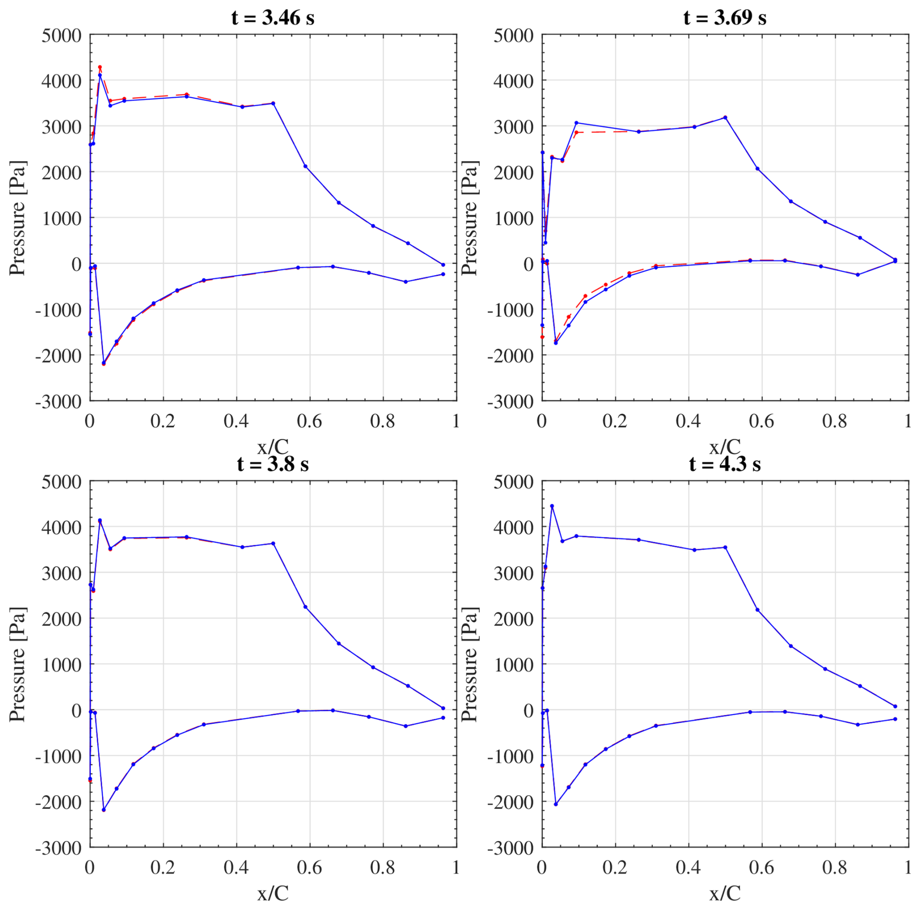
Figure 22 Blade surface pressure distributions, where blue is the raw measurement and red is the reconstructed measurement, at different times during blade passage: t = 3.46 s (just before passage), t = 3.69 s (at passage), t = 3.80 s (just after passage), and t = 4.30 s (in the middle of a passage).

4.5.4 Comparison of pressure measurements with aeroelastic simulations

The OpenFAST model was run to estimate the forces normal to the chord at the two blade spanwise locations where the two belts are installed. Six turbulent seeds of 10 min simulations were run to represent conditions measured in the field in terms of average wind speed, average turbulence intensity, and average shear exponent. The comparison between numerical predictions and experimental measurements from the first day of measurements is shown in Fig. 23. The plots display average values as solid lines and standard deviation as a shaded area. In addition to an offset between the two average lines, OpenFAST predicts deeper effects caused by the blade/tower interaction, which is estimated via the conventional Powles shadow model. Simulations were repeated, adopting the Eames model to predict tower shadow (Simpson et al., 2022; Eames et al., 2011) and varying the drag coefficient along the tower, with no notable improvement. Note that the above observations may be somewhat frustrated by effects from azimuthal binning that tend to smear the actual dynamics of the blade during individual tower passages (Madsen et al., 2007); this situation is evidenced by the large standard deviation of the measured data around the blade/tower interaction.

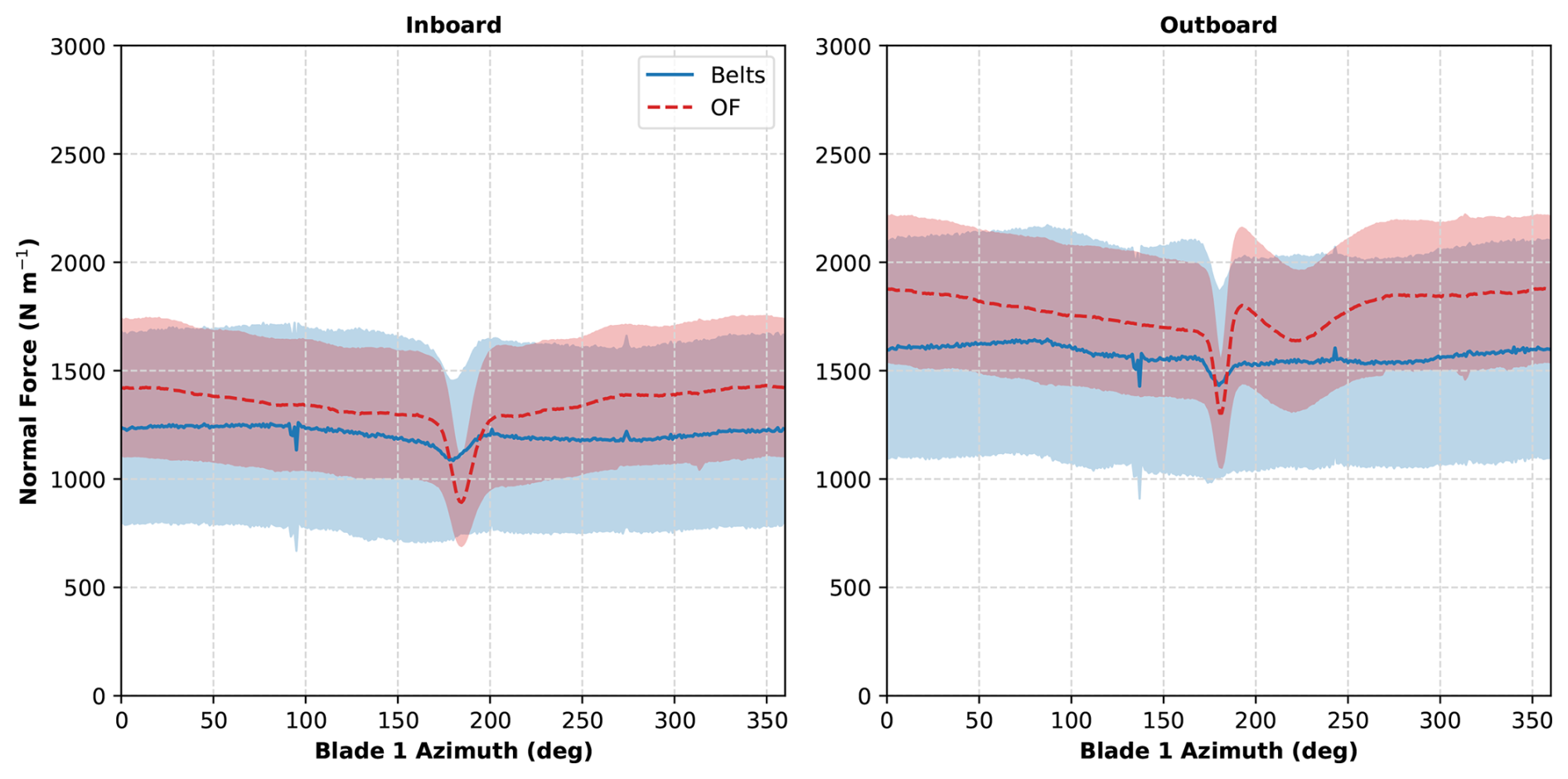
Figure 23 Comparison of normal forces between numerical predictions from OpenFAST and experimental measurements from the belts for (left) inboard and (right) outboard belts. The shaded area represents 1 standard deviation. Data are only from the first day of measurements.

The observations above should also be interpreted in light of the unsteady aerodynamic effects from shed vorticity and apparent mass associated with the passage of the blade through the tower shadow, which produced effective reduced frequencies well above 0.05 and 0.2 for the outboard and inboard sections, respectively, where the effective frequency was calculated based on the duration of the normal-force disturbance around the blade/tower interaction event. These reduced frequencies qualify as moderately to highly unsteady, respectively, and it has been shown previously that attached-flow unsteady loading effects in these regimes cause an attenuation and delay of the maximum normal force disturbance of an airfoil section passing through the tower shadow as compared to quasi-steady aerodynamics (Leishman, 2006). Studies suggest that the validation success of indicial gust-response loading models (such as the Beddoes–Leishman-derived model employed in this article) applied to impinging wakes is sensitive to the accuracy of the reconstruction of the incoming wake profile (Munduate et al., 2004; Wang and Coton, 2001; Noyes et al., 2018; Brown et al., 2021), though both tower shadow models tested produced similar overpredictions of the amplitude of the disturbance, granted uncertainties due to the azimuthal binning process. Looking ahead, leveraging the inflow time series measured by the five-hole probe during (phase-aligned) tower passages may help indicate whether validation error is being introduced by the modeling of the tower shadow and/or the modeling of unsteady blade aerodynamic effects.

It should also be noted that at the unusually small blade/tower clearance of this experiment, the assumption of a one-way decoupled interaction, where the tower wake acts as an incoming disturbance to the blade without the blade's pressure field in turn modifying the tower flow, may not be fully justified. At such close proximity, two-way aerodynamic coupling between blade and tower could represent an additional source of modeling error beyond the two already identified. The full three-dimensional CFD rotor simulations including tower flow mentioned above are the appropriate tool to assess the significance of this coupling.

5 Discussion

Although challenged by the weather conditions during the planned experimental campaign over 2 weeks in the second half of April 2024, we succeeded in conducting two campaigns, about 5 and 1 h in length. On the first day the wind speed varied so that the turbine operated throughout its entire regime from start-up to rated power. In spite of narrow filters on measured power, pitch and yaw error blade pressure coefficients have been derived for four angles of attack: 4, 6, 8, and 10°. Compared with 2D CFD simulations of the pressure coefficients in Fig. 14, we find a close correlation on the outboard section but some deviation at an angle of attack of 4°. It seems that the measurements might be measured at a slightly higher angle of attack than 4°, which was derived based on the 2D upwash correction.

At the inboard section, the deviations are more pronounced and are again greater for lower angles of attack of 4, 6, and 8° (Fig. 13). Again, this could be due to differences in the angle of attack in the measured and simulated pressure distributions but also to three-dimensional flow effects and the roughness of the blade, which might explain the missing simulated suction peak at 8 and 10°.

However, the measured data are well suited for use in the detailed validation of high-fidelity simulation tools such as 3D CFD rotor simulations. The discussion of uncertainties in conversion of inflow angle to angle of attack is not as important because the local inflow angle at the position of the five-hole probe can be compared directly with the inflow angle extracted from the CFD simulations and used, for example, to tune the free wind speed in the CFD simulations. Many different validation cases are believed to be defined for future use of the experimental data, for example, showing the detailed pressure variation on the tower and the blade surface during the blade passage, as illustrated experimentally in Figs. 21 and 22.

Such CFD rotor simulations should then also include tower flow modeling like the simulations by Zahle et al. (2009) and Klein et al. (2018) and contribute to quantifying the importance of the tower as an acoustic transmitter. In the present measurements, we found typical impulsive forces on the tower in the range of 100–150 N m⁻¹ and impulsive blade forces in the range 200–500 N m⁻¹.

6 Conclusions

We performed a detailed experimental characterization of the flow characteristics of the blade/tower interaction of a downwind rotor using a novel add-on measurement system on one blade and on the tower that consisted of pressure belts, two five-hole probes, and two data acquisition systems. The measurement campaign was part of a comprehensive project at NREL to support investigations on the feasibility, reliability, performance, and economic viability of wind turbines oriented downwind. The instrumentation at two sections on the blade was successfully installed on the 1.5 MW turbine at NREL's Flatirons Campus. In a first measurement campaign before the pressure belt on the tower was installed, pressure and inflow data at the two blade stations were measured over about 5 h with the turbine operating from cut-in to rated wind speed.

The preliminary analysis of the blade pressure distribution and inflow data indicated that the data are of good quality and thus well suited for use in validating high-fidelity simulation codes such as 3D CFD rotor models. A good demonstration of the value of the detailed pressure measurement is that the lower lift coefficient on the inboard section at a high angle of attack can be explained by the missing suction peak in the pressure distribution, perhaps due to operation in atmospheric and wind tunnel flow.

At the end of the campaign we succeeded in installing the pressure belt on the tower and obtained about 1 h of pressure data on the tower and from the outboard blade section passing at the same height as the pressure belt on the tower. The initial analysis of these unique data on a full-scale downwind rotor showed impulsive loading on the tower in the range of 100–150 N m⁻¹ and on the blade section in the range of 200–500 N m⁻¹. A dynamic correction method to compensate for the response lag in the longest channels (up to about 10.7 m) of the tower pressure belt showed large changes in the reconstructed data (both pressure magnitude and timing), whereas for the sampling rates used here, only minor changes were seen in the reconstructed pressure measurements on the blade sections due to the much shorter pressure belts.