Classification of leading-edge-erosion severity via machine learning surrogate models

Leading-edge erosion is a common form of wind turbine blade deterioration that reduces aerodynamic performance, increases maintenance demands, and shortens turbine service life. Machine-learning-based structural health monitoring systems offer a promising route for detecting erosion severity, but their performance often depends on access to large labeled training datasets. For wind turbine applications, generating these datasets with full-physics simulation can be computationally expensive, motivating the use of surrogate models for efficient data generation.

In this work, we evaluate whether a Gaussian process (GP) emulator can replace full-physics simulation as a training-data generator for leading-edge-erosion classification. The surrogate is trained on a limited set of OpenFAST simulations and then used to generate large labeled datasets, essentially cost-free, for a random forest classifier. We apply a parallel partial and zero-censored emulator which extends the standard GP framework by predicting a vector of response statistics associated with aerodynamic, structural, and turbine-level outputs and incorporating output constraints to improve the physical consistency and uncertainty calibration of the predictions.

We compare two random forest classifiers: one trained directly on full simulation data and one trained on emulator-generated data. Both classifiers are evaluated on held-out full-physics simulation data across five leading-edge-erosion severity levels. The emulator-trained classifier achieves accuracy comparable to the simulator-trained classifier, demonstrating that the GP surrogate can substantially reduce the cost of training-data generation without sacrificing classification performance. These results suggest that constrained, vector-valued GP emulators can support efficient simulation-based structural health monitoring workflows and may provide a useful component of future digital-twin frameworks for wind turbine maintenance.

1 Introduction

Wind energy plays a crucial role in the worldwide transition to renewable sources of energy (Hassan et al., 2024; Bošnjaković et al., 2022). Reducing the cost of energy over the lifetime of a wind turbine (WT) requires reducing operation and maintenance (O&M) costs (Myhr et al., 2014; Park et al., 2022; Ren et al., 2021). Opportunities to reduce O&M include maintaining new offshore WTs, operating aging land-based WTs (Bilgili and Alphan, 2022; Veers et al., 2019), and monitoring large-scale WTs with flexible blades and high tip speeds (Barlas and van Kuik, 2010).

Leading-edge erosion (LEE) is a driver of O&M costs (Maniaci et al., 2022). LEE creates structural risks that may necessitate the complete replacement of WT blades (Maniaci et al., 2022). Offshore turbines face an elevated risk for LEE due to harsh environmental exposure (Shankar Verma et al., 2021b), and large-scale rotors are expected to erode faster on their blade tips due to the increased tip speeds (Carraro et al., 2022; Haus, 2020). Studies suggest erosion-related energy losses range from 2 % to 3.7 % annually (Han et al., 2018). While there are many approaches to mitigate LEE (Antoniou et al., 2022; Herring et al., 2019; Macdonald et al., 2016; Pryor et al., 2022; López et al., 2023; Shankar Verma et al., 2021a; Visbech et al., 2023), non-destructive evaluation (NDE) techniques, including visual inspection, ultrasonic testing, thermography, acoustic emission monitoring, vibration-based monitoring, and supervisory control and data acquisition (SCADA)-based signal processing (Civera and Surace, 2022), have shown promise towards reducing O&M costs by limiting turbine downtime while preventing damage from developing unnoticed. The proactive detection and mitigation of LEE minimizes energy loss and avoids full blade replacement (Campobasso et al., 2023; Tchakoua et al., 2014).

Structural health monitoring (SHM) for LEE remains challenging (Mishnaevsky, 2022). Visual inspection may only detect defects after substantial degradation has occurred (Pugh et al., 2021). Improvements in UAV-based blade surveillance (Shihavuddin et al., 2019) and gloss-based surface characterization (Leishman et al., 2022) still require devices in close proximity to WT structures in order to work. Alternatively, SCADA-based methods (Maldonado-Correa et al., 2020; Pandit et al., 2023) rely on available data gathered without the need for workers or instruments to be moved into physical proximity to the blades. Along with sensors for blade load measurements (Abdallah et al., 2015) and aerodynamic surface pressure (Duthé et al., 2021) measurements, SCADA signal processing, combined with machine learning (ML) methods, is showing promise for driving down the O&M cost of LEE (Maldonado-Correa et al., 2020; Pandit et al., 2023).

Machine learning (ML) has proven to be useful for SHM through analyzing SCADA data for turbine fault detection and blade damage (Du et al., 2020; Stetco et al., 2019; Zaher et al., 2009; Jiménez et al., 2017). ML techniques, including random forest (Fezai et al., 2020), XGBoost (Zhang et al., 2018), and neural networks (NNs) (Chen et al., 2021; Choe et al., 2021), have successfully detected faults in SHM data. Additionally, ML is being applied to SHM problems for LEE detection. Applications include the use of NN to predict energy loss from eroded blades (Campobasso et al., 2020), the coupling of computational fluid dynamics (CFD) simulators with aero-elastic modeling to simulate erosion patterns and quantify damage (Enríquez Zárate et al., 2022), transformer models to track erosion severity in turbulent conditions (Duthé et al., 2021), and deep learning to predict LEE using aerodynamic data (Abdallah et al., 2022; Carmona-Troyo et al., 2025).

Although ML is a promising avenue for detecting LEE, its effectiveness is constrained by the need to collect large volumes of high-fidelity training data (Ward et al., 2024). Data generation can impose a computational bottleneck for training and validating these systems. For instance, CFD simulations with fine-scale aerodynamic effects of erosion require computationally expensive numerical solutions to the Navier–Stokes equations, which is not feasible for a large dataset generation (Langel et al., 2017). Even reduced-order modeling approaches are prohibitively costly when simulating erosion under diverse atmospheric conditions (Carraro et al., 2022). While aero-elastic simulations offer a more tractable alternative, studies demonstrate that the impact of blade damage is affected by wind speed, turbulence intensity, and air density, necessitating extensive dataset coverage of operational scenarios for reliable model generalization (Pandit et al., 2023; Papi et al., 2020). In this study, we address a central limitation of ML-based SHM by reducing the computational cost of generating sufficiently large labeled datasets from full-physics aero-elastic models. We show that a computationally inexpensive GP emulator can be trained on a limited set of simulations and then used to generate large datasets to train LEE classifiers while preserving classification performance when evaluated on held-out ground truth simulation data.

Surrogate modeling is commonly employed to address complexity and scalability challenges in WT engineering by providing a computationally efficient approach to damage tracking and predictive maintenance (Clark and Clark, 2022; Golparvar et al., 2021; Murcia et al., 2018; Singh et al., 2024). Surrogate modeling approaches encompass several techniques, but Gaussian process (GP) emulators are the most popular choice (Murcia et al., 2018; Singh et al., 2024). GPs are frequently used for uncertainty quantification, calibration, power or load prediction, SHM, and reliability analysis (Golparvar et al., 2021; Clark and Clark, 2022; Rogers et al., 2020; Avendano-Valencia et al., 2020; Abdallah et al., 2019). GP applications include multi-fidelity kriging, damage-equivalent load estimation, and the fusion of synthetic and real data (Abdallah et al., 2019; Avendaño-Valencia et al., 2021; Haghi et al., 2024). However, the existing GP literature primarily focuses on predicting scalar or low-dimensional quantities of interest. Emulation for SHM requires physically consistent, higher-dimensional outputs for downstream tasks such as damage classification. With the standard approach, emulating a WT simulator that generates higher-dimensional vector-valued output from multiple sensor channels requires separately fitting and storing multiple standard scalar GPs, one for each output dimension. In this paper we use partial parallel emulation to significantly accelerate the prediction of vector-valued outputs (Gu and Berger, 2016). In addition, for outputs with constraints, such as generator power, a standard GP is unrealistic because its output is unbounded. Spiller et al. (2023) developed the zero-censored GP emulator to enforce range-limited outputs. We show that the combination of parallel partial and zero-censored emulation (PPzGP) (Gu and Berger, 2016; Spiller et al., 2023) improves the fidelity and computational efficiency of higher-dimensional WT emulation models.

Our primary contribution in this paper is the introduction of a framework to reduce the computational cost of training a SHM monitoring algorithm. Specifically, we present the first application of the PPzGP emulation methodology to wind turbine modeling and the classification of LEE. While this work involves simplifications to the physics and operating conditions, including assuming steady-state wind, the approach could be extended to more physically realistic scenarios, including turbulent inflow. We compare the performance of LEE classifiers trained on datasets generated from the emulator to those obtained using OpenFAST simulations. Our PPzGP emulator reduces the computational cost of acquiring training data and improves accuracy compared to training the classifier using OpenFAST simulations. The PPzGP is also significantly more efficient than training multiple standard scalar GP emulators for each output quantity of interest. Once fit, the cost of using the GP emulator to generate SHM classifier training data is essentially free. In our experiments, the classification results show generated data can be used without a significant loss of accuracy (emulator-trained classifiers: 0.88 macro-F1; OpenFAST trained classifiers: 0.82 macro-F1). The computational savings are significant. Including the cost of running the simulator to produce the training data for the emulator, the overall computational time is drastically reduced. Performance improvements are greatest for the intermediate erosion classes, implying that the larger emulator-generated training set is especially beneficial for resolving the more ambiguous LEE class boundaries.

2 Methods

In this section, we describe the workflow used to test whether emulator-generated data can replace direct simulations for training LEE classifiers. We use OpenFAST (Golparvar et al., 2021; Jonkman et al., 2024; Moynihan et al., 2022; Murcia et al., 2018) to simulate the NREL 5 MW reference turbine under varying environmental conditions and stochastic LEE states. We use global sensitivity analysis (Morris, 1991) to identify influential simulator inputs. Finally, we train a vector-valued GP emulator (Smith, 2024) with parallel partial emulation (Gu and Berger, 2016) and zero-censored treatment (Spiller et al., 2023) of range-limited outputs, generate large emulator-based training datasets, and compare the resulting random forest (Breiman, 2001) classifier performance with that of the simulation-trained classifier. Both classifiers are evaluated on held-out simulations so that the full aeroelastic model provides the reference test data.

2.1 OpenFAST

The OpenFAST wind turbine simulator is developed and maintained by the National Laboratory of the Rockies (NLR) for a wide range of aerodynamic and structural applications. OpenFAST simulates the response of a wind turbine to environmental conditions by linking specialized structural and physical modules, including those for wind flow, aerodynamics, structural dynamics, and servo-dynamics (Jonkman, 2013; Rinker et al., 2020). OpenFAST has been applied to supply realistic aero-servo-elastic data for LEE detection, including the generation of blade tip accelerometer data (Enríquez Zárate et al., 2022) and lift or drag sensor data (Duthé et al., 2021).

Because of its versatility and well-established capabilities, we use OpenFAST to generate realistic LEE data, relying on the coupling of four OpenFAST modules: AeroDyn, ElastoDyn, ServoDyn, and InflowWind. These modules contribute to the simulation of blade forces, including lift and drag, blade loads, generator power, and the wind environment. The InflowWind module calculates the wind vectors around the turbine while taking into account the turbine's size and hub height. InflowWind can simulate wind fields with a variety of properties. In this study we use uniform wind fields, include wind shear, and specify wind direction. Aerodynamic forces and blade loads, handled by the module AeroDyn, are particularly important for LEE. AeroDyn uses blade element momentum theory (BEM) (Jonkman et al., 2015) to calculate aerodynamic forces on the rotor by breaking the blade into discrete regions or elements. These elements are assigned a lift or drag coefficient according to their instantaneous angle of attack with the oncoming air. The relationship between the angle of attack and lift or drag is modeled using aerodynamic polar curves. OpenFAST uses a look-up table based on the polar curve to calculate torque and thrust forces on the axial shaft of the wind turbine (Ning, 2014; López et al., 2023). ServoDyn regulates the electronic systems of the wind turbine using structural motions, loads, and wind measurements; calculates the power generation; and determines control responses. In this study, the nacelle is fixed, but we enable the servo-controller to pitch the blades and regulate the rotor, in order to maximize power below rated wind speed and maintain rated power above rated wind speed. The default wind turbine controller model has variable speed and collective pitch control, which regulates the power generated as a function of the wind speed by pitching the wind turbine blades and controlling the rotor torque to maximize power below the rated wind speed (Abbas et al., 2022). Aerodynamic changes due to LEE result in changes in the dynamics of the blade. These effects are modeled using the ElastoDyn module, which calculates the blade and tower displacement, velocity, and acceleration and allows for the simulation of accelerometers at the tips of the blades and loads at the root of the blades. ElastoDyn uses several different input parameters, including the blade geometry, the mass or inertia of blade elements, and the stiffness of elements.

2.2 Leading-edge-erosion data generation

All datasets in this study were generated with the 5 MW reference wind turbine in OpenFAST using the AeroDyn, ElastoDyn, ServoDyn, and InflowWind modules (Jonkman et al., 2009). The wind speed, direction, air density, and shear (see Table 1) are held fixed during each run.

Table 1 OpenFAST NREL 5 MW reference WT (RWT) upwind three-blade WT simulation model parameters.

The wind speed ranges from the lowest speed at which the turbine generates power to the speed where the blades are stalled to prevent damage (cut-in to cut-out wind speeds) for the 5 MW reference wind turbine (see Table 1) (Jonkman et al., 2009). Because air density has a large impact on power (Golparvar et al., 2021), we use a wide range of air densities, based on a conservative lower bound expected in cold, low-humidity conditions at around sea level up to realistic high temperatures for turbines in onshore environments (Liang et al., 2020). We model wind speed, V, as a function of height, h, above the ground using the wind shear power law (Platt et al., 2016) $V\left(h\right)=V_{\text{r}}{\left(\frac{h}{h_{\text{r}}}\right)}^{\mathit{\nu }}$, where V_r is the reference wind speed, h_r is the hub height (see Table 1), and ν is the shear parameter. The nominal wind shear parameter depends on the topographic surroundings of the turbine. We set a value of ν=0.2 as the default wind shear parameter (Liu et al., 2024). In Table 2 we summarize the ranges of the environmental parameters. To ensure that the turbine reaches equilibrium with the environmental conditions, we ran the simulations for 180 s and discarded the first two-thirds of simulation times to avoid transient effects (Golparvar et al., 2021).

Table 2 Environmental variable ranges.

2.2.1 Leading-edge-erosion model

LEE is primarily driven by material stresses due to the collision of particles (e.g., rain drops) with the blade surface (Bech et al., 2018; Pryor et al., 2022). This has the effect of damaging the blade coating, ultimately leading to surface roughening and the growth of pits and gouges (Pryor et al., 2022). As the blade is roughened, the transition between laminar and turbulent airflow shifts, (Panthi and Iungo, 2023), reducing lift and increasing drag (Gaudern, 2014). Rather than using computationally expensive CFD simulations to model airflow over rough surfaces, for the results in this paper we adapt a phenomenological LEE model developed by Duthé et al. (2021) that is straightforward to implement within the AeroDyn module of OpenFAST. With this simplified model, the effect that erosion has on the aerodynamic properties of the blade edge is represented via a spatial perturbation of the lift and drag polars as a function of the angle of attack. Duthé et al. (2021) based these perturbations on wind tunnel experiments (Han et al., 2018) in which erosion defects were simulated using roughened tape applied to the blade (Zidane et al., 2016).

As in Duthé et al. (2021), we quantify the severity of erosion using a finite ordered set of damage classes, which encode the overall erosion level of the blade. These classes provide a practical link between observed surface degradation, aerodynamic performance loss, and potential remedial actions (Han et al., 2018; Sareen et al., 2014; Maniaci et al., 2022).

Although we do not model the time evolution of erosion, the idea is that erosion severity will be greater for older blades that have experienced more impact events. In addition, it is reasonable to assume that, to first order, the amount of erosion depends linearly on position along the blade. This erosion is expected to initiate and progress more rapidly in blade regions that are further from the hub (Bech et al., 2018; Maniaci et al., 2022; Schramm et al., 2017; Verma et al., 2020). Finally, to take into account the inherent variability in erosion, we model the spatial dependence of erosion stochastically (Duthé et al., 2021).

We now describe the details of this erosion model. For this study, we use five erosion severity classes parameterized by $\mathit{\alpha }\in \mathit{\{}\mathrm{0.00},\mathrm{0.25},\mathrm{0.50},\mathrm{0.75},\mathrm{1.00}\mathit{\}}$. We divide the blade into six erosion regions via a grouping of the AeroDyn nodes defined in the NREL 5MW RWT (see Table 1; Jonkman et al., 2009) summarized in Table 3 and shown in Fig. 1. We let $e_i\in [\mathrm{0},\mathrm{1}]$ denote the erosion level of the ith blade region, where e_i=0 corresponds to a clean surface, and e_i=1 corresponds to the maximum modeled erosion state. We model the erosion vector as a correlated random field,

$$\mathbf{e}=(e_{\mathrm{1}},\mathrm{\cdots },e_{\mathrm{6}})\sim \mathrm{MVN}\left(\mathit{\mu }\right(\mathit{\alpha }),\mathbf{\Sigma }(\mathit{\alpha }\left)\right),$$

where both the mean and covariance depend on the erosion severity class, α. To incorporate the linear relationship between blade velocity and radial distance into the model, we define the mean erosion level by

$$\mathit{\mu }\left(\mathit{\alpha }\right)=(\mathit{\alpha }{x}_{\mathrm{1}},\mathrm{\dots },\mathit{\alpha }{x}_{\mathrm{6}}),$$

where x_i is the normalized radial distance from the hub to the midpoint of the ith blade region. The covariance matrix is defined by

$$\mathbf{\Sigma }(\mathit{\alpha }{)}_{i,j}={\left({\displaystyle \frac{min(x_i,x_j)\mathit{\alpha }}{\mathrm{10}}}\right)}^{\mathrm{2}}\exp \left({\displaystyle \frac{-(x_i-x_j{)}^{\mathrm{2}}}{x_i+x_j}}\right).$$

This heuristic covariance model imposes stronger correlation between the erosion level in nearby blade regions while allowing erosion variability to increase both toward the blade tip and with erosion severity. The increase in erosion variability with erosion severity accounts for the fact that severe erosion can be due to a range of physical states, including coating loss, roughness patches, pits, gouges, and localized defects, whereas mild erosion is comparatively more uniform (Maniaci et al., 2022). This model takes values sampled from the normal distribution that lie in the interval [0,1], replacing values that are <0 by 0 and values >1 by 1.

Figure 1 Diagram of erosion regions described in Table 3. The red square shows the location of the aerodynamic node where lift and drag sensor data are measured. The y axis measures $r/R$, the relative proportion of the total blade length; see Table 3.

Once we have sampled the erosion levels, e_i, we model the aerodynamic effect of erosion through a simplified spatial perturbation of the lift and drag polars. This approach is consistent with prior erosion models that interpolate or perturb aerodynamic polars according to local damage severity (Maniaci et al., 2022; Abdallah et al., 2015). Based on reported severe-erosion effects, including lift losses up to 53 % (Han et al., 2018) and drag increases up to 500 % (Sareen et al., 2014), we scale the lift and drag coefficients in the ith blade region according to $c_{\mathrm{L},i}=\mathrm{1}-\mathrm{0.53}{e}_i$ and $c_{\mathrm{D},i}=\mathrm{1}+\mathrm{4}{e}_i$.

Table 3 Blade erosion regions, defined by the aerodynamic nodes of the 5 MW NREL reference turbine. Node 18 is used to track aerodynamic data.

This simplified erosion model has several limitations. First, our model lacks realistic temporal resolution of erosion. More detailed stochastic models represent erosion as a random accumulation process, where damage arrival and severity depend on quantities such as blade radius, wind speed, precipitation, and exposure history (Duthé et al., 2021). In addition, experimental descriptions of liquid droplet erosion often identify a multi-stage progression, including an incubation period with little apparent mass loss and a nonlinear acceleration phase, followed by an approximately linear damage–growth regime (Law and Koutsos, 2020). By contrast, the present model assigns blades directly to ordered erosion classes and does not attempt to reproduce these intermediate growth dynamics.

Second, we use a simplified aerodynamic perturbation model which interpolates between clean and maximally eroded behavior using scalar modifications to the lift and drag coefficients. In reality, surface roughness can alter the shape of lift and drag polars in an angle-of-attack-dependent and nonlinear manner. For example, Abdallah et al. (2015) model eroded lift polars using multiple aerodynamic parameters, while Duthé et al. (2021) show that erosion effects may be negligible over some angle-of-attack ranges. A more detailed modeling approach would explicitly modify the blade surface geometry, compute the resulting aerodynamic polars using CFD, and then pass the modified polars to a turbine-level simulator (Enríquez Zárate et al., 2022).

Finally, our use of five erosion classes necessarily coarsens a gradual physical process. This representation does not resolve subtle differences between early-stage erosion states or the full diversity of possible damage patterns along the blade. However, our simplified stochastic parameterization is not intended to model the complete time evolution of LEE. Rather, it is designed to generate physically motivated families of aerodynamic perturbations for evaluating whether emulator-generated data can support erosion-severity classification. For this purpose, the model preserves several important qualitative features. Namely, (1) erosion damage increases monotonically with class severity, (2) erosion accumulation is weighted toward the tip, and (3) the induced aerodynamic changes reduce lift and increase drag within reported ranges. Since practical erosion assessment often relies on coarse-level observed blade deterioration, which is then connected to performance loss and maintenance decisions (Maniaci et al., 2022), this class-based proxy provides a useful proof-of-concept setting for testing the proposed emulator-based workflow.

2.2.2 Sensors

We use five sensors to monitor erosion damage: generator power, aerodynamic lift and drag, blade tip acceleration, and blade root force moment (Duthé et al., 2021; Enríquez Zárate et al., 2022). Although lift and drag measurements are not commonly available, new sensors under development (Barber et al., 2022) measure aerodynamic pressure over an aero-foil section to calculate the dynamic lift coefficient, which can be used to detect changes in airflow patterns due to surface roughness (Abdallah et al., 2022). Similar studies have used these data to track the progression of LEE using OpenFAST software (Abdallah et al., 2022; Duthé et al., 2021). Note that we only track lift and drag at the tip of the blade, AeroDyn Node 18, since it is the location where erosion will accumulate most rapidly (Duthé et al., 2021).

Since aerodynamic changes alter blade kinematics, we track flap-wise acceleration of the tip of the blade, used by Du et al. (2020) and Enríquez Zárate et al. (2022), and the edge-wise moment of the root of the blade, used by Moynihan et al. (2022) and Sheibat-Othman et al. (2015).

We use feature extraction to reduce the dimension of the time series outputs from our OpenFAST simulation, a vector with 160 entries per second of simulation time per sensor. Following a similar approach to Enríquez Zárate et al. (2022), we use statistical moments of each of the five output time series, specifically the mean, standard deviation, skew, and kurtosis (Kaewniam et al., 2022), rather than the time series itself.

Enríquez Zárate et al. (2022) also extracted richer features from time series data such as higher-order crossings, mobility, and complexity features, but in Sect. 4 in Figs. 8 and 9 we show high classification accuracy without additional feature extraction. A plausible reason for this may be that (1) we look at a relatively coarse set of erosion levels that naturally have distinct features because they do not naturally overlap, and (2) we are using bulk output statistical features which contain a large amount of information for steady-state wind flow. In Table 4 we summarize the simulator outputs, along with their variable names in OpenFAST and their units. These quantities are the inputs to the random forest classifier which we use to determine erosion accumulation damage.

Table 4 Simulated sensor outputs.

2.3 Global sensitivity analysis

Global sensitivity analysis (GSA) identifies inputs which drive significant variation in the simulator outputs (Smith, 2024). By using GSA to fix non-influential inputs, fewer simulations are required to train an accurate emulator. Morris (1991) proposed the elementary effect method (Morris screening) as an efficient GSA method for high-dimensional, nonlinear, and computationally expensive models. Velarde et al. (2019) used elementary effect analysis to determine the relative importance of input parameters for analyzing the foundation loads of offshore wind turbines.

To apply the elementary effect analysis, the input space, 𝓤, is first scaled to the p-dimensional unit hypercube, which is partitioned into a grid with spacing Δ. A random sample of r initial input points, ${\mathit{u}}_{\mathrm{0}}^{\left(j\right)}\text{ for }j=\mathrm{1},\mathrm{\dots },r$, is taken from these grid points. Starting at each of these random points, a sequence of p points is generated by applying p unit changes to the input dimensions in a random order to create the elementary effect experiment design. For each component index l of u and each of the r trajectories indexed by j, the method calculates the elementary effect using a finite difference:

$$\begin{array}{}\text{(1)}& {\mathrm{EE}}_{l,j}\left(\mathbf{u}\right)=\left[f\right(\mathit{u}+{\mathbf{e}}_l)-f(\mathit{u}\left)\right]/\mathrm{\Delta }.\end{array}$$

The mean and the standard deviation of the elementary effects, $\mathit{\{}{\mathrm{EE}}_{l,\mathrm{1}},\mathrm{\dots },{\mathrm{EE}}_{l,r}\mathit{\}}$, are calculated for each dimension l. To avoid the possibility of large positive and negative elementary effects canceling out, we use ${\mathit{\mu }}_l^{*}=\frac{\mathrm{1}}{r}{\sum }_{j=\mathrm{1}}^r\left|{\mathrm{EE}}_{l,j}\right|$ instead of the mean, μ_l. The standard deviation, which requires the average of elementary effects, μ_l, is given by ${\mathit{\sigma }}_l=\sqrt{\frac{\mathrm{1}}{r}{\sum }_{j=\mathrm{1}}^r({\mathrm{EE}}_{l,j}-{\mathit{\mu }}_l{)}^{\mathrm{2}}}$ (Iwanaga et al., 2022). A large mean elementary effect, ${\mathit{\mu }}_l^{*}$, indicates that the l^th input has a large overall effect, while a large σ_l indicates strong nonlinear effects or interactions with the other inputs (Cropp and Braddock, 2002). A plot of pairs $({\mathit{\mu }}_l^{*},{\mathit{\sigma }}_l)$ for each input $l\in \mathit{\{}\mathrm{1},\mathrm{\dots },p\mathit{\}}$ is used to determine the relative importance of the inputs (Campolongo et al., 2007; Morris, 1991). We use the elementary effect tool provided in the Python library SALib (Herman and Usher, 2017; Iwanaga et al., 2022).

2.4 Gaussian process emulation

In this section we review Gaussian process (GP) emulation. For several decades GP emulation has been applied to problems from domains as varied as thermal energy storage (Currin, 1988), electrical circuits (Welch et al., 1992), and the design of chemical experiments (Sacks et al., 1989). GP emulators were introduced to reduce the computational cost of repeatedly evaluating complex numerical models. They are especially useful when the computational cost of a single simulation is high and when an extremely large number of simulations are required. The GP emulator is trained on a limited number of simulations run at design points. Once trained, the GP acts as an interpolator between design points in input space so that evaluating the output quantity of interest (QoI) at untested inputs is essentially free. Therefore, it is feasible to generate much larger training datasets for subsequent machine learning algorithms via an emulator than would be possible using the full simulator. The GP also provides uncertainty quantification for evaluations at new inputs via credible intervals which assess the accuracy of the emulator as a surrogate model for the full physical simulator.

For wind turbine condition monitoring, building training sets for damage classification requires evaluating the simulator hundreds to thousands of times, which can be computationally prohibitive. Steady-state simulations in OpenFAST take on the order of minutes on a typical laptop/desktop computer, while turbulent wind and wave simulations in offshore environments take much longer. GPs are good approximations of simulators that vary smoothly as a function of inputs, which is the case for wind turbines (Rinker, 2016). Further, prediction and uncertainty estimation are robust in the presence of limited data (as compared to neural networks, for example) (Myren and Lawrence, 2021).

2.4.1 Scalar Gaussian process emulation

We begin with a discussion of the basic GP formalism and then describe the extensions we employ for emulation of wind turbines. For scalar-valued output, the wind turbine simulator is treated as a function, f, from the space of input parameters, $\mathit{u}\in \mathcal{U}\subset {\mathbb{R}}^p$, to the output quantity of interest, $v\in \mathcal{V}\subset \mathbb{R}$. For wind turbine erosion modeling, inputs include (for example) the wind velocity and the blade damage level, with generator power as an output. The unknown deterministic function $f:\mathcal{U}\to \mathcal{V}$ is then modeled as a draw from a random Gaussian process (GP), $\stackrel{\mathrm{̃}}{f}$, with the property that for any finite subset, $\mathit{\{}{\mathit{u}}_{\mathrm{1}},\mathrm{\dots },{\mathit{u}}_n\mathit{\}}\in$ 𝓤, the random variables, $\mathit{\left\{}\stackrel{\mathrm{̃}}{f}\right({\mathit{u}}_{\mathrm{1}}),\mathrm{\dots },\stackrel{\mathrm{̃}}{f}({\mathit{u}}_n\left)\mathit{\right\}}\in \mathcal{V}$, follow a multivariate Gaussian distribution (Rasmussen, 2003). The modeling begins with the assumption of a GP prior with a mean trend $\mathit{\mu }:\mathcal{U}\to \mathcal{V}$ and covariance $C:\mathcal{U}\times \mathcal{U}\to \mathbb{R}$. The mean trend is of the form μ(u)=h^T(u)θ for some choice of q basis functions (often taken to be a constant or linear function of the input parameters), $\mathit{h}\left(\mathit{u}\right)=\left(h_{\mathrm{1}}\right(\mathit{u}),\mathrm{\dots },h_q(\mathit{u}){)}^T$, and regression coefficients, θ. The covariance is of the form $C({\mathit{u}}_{\mathrm{1}},{\mathit{u}}_{\mathrm{2}})={\mathit{\sigma }}^{\mathrm{2}}c({\mathit{u}}_{\mathrm{1}},{\mathit{u}}_{\mathrm{2}})$, where σ² is the variance (output scaling) of the GP, and $c:\mathcal{U}\times \mathcal{U}\to \mathbb{R}$ is the correlation function, which is specified by the choice of a kernel (Rasmussen, 2003; Santner et al., 2003). In this work we use the Matérn $\mathrm{5}/\mathrm{2}$ kernel (Stein, 1999, Gu et al., 2018, Spiller et al., 2023) given by $c({\mathit{u}}_{\mathrm{1}},{\mathit{u}}_{\mathrm{2}})={\prod }_{k=\mathrm{1}}^p(\mathrm{1}+\sqrt{\mathrm{5}}{d}_k+\frac{\mathrm{5}}{\mathrm{3}}{d}_k^{\mathrm{2}})\exp (-\sqrt{\mathrm{5}}{d}_k)$. Here $d_k=\frac{\mathrm{1}}{{\mathit{\gamma }}_k}|u_{\mathrm{1},k}-u_{\mathrm{2},k}|$ is a normalized distance between the kth entries of the vectors u₁ and u₂. The correlation coefficients, $\mathit{\gamma }=({\mathit{\gamma }}_{\mathrm{1}},{\mathit{\gamma }}_{\mathrm{2}},\mathrm{\dots },{\mathit{\gamma }}_p{)}^T$, determine how rapidly the emulated output changes with respect to each input dimension. Letting ${\mathbf{U}}_i^{\mathrm{D}}$ $(i=\mathrm{1},\mathrm{\dots },n)$ represent the design of training inputs (e.g., different settings of wind speed and blade damage), the corresponding response vector of outputs (power generated for each setting) is given by ${\mathbf{v}}^{\mathrm{D}}=(v_{\mathrm{1}}^{\mathrm{D}},\mathrm{\dots },v_n^{\mathrm{D}}{)}^T$. We denote the training input/response data together as ${\mathcal{D}}_{\text{GP}}=\mathit{\left\{}\right({\mathbf{U}}_{\mathrm{1}}^{\mathrm{D}},v_{\mathrm{1}}^{\mathrm{D}}),\mathrm{\dots },({\mathbf{U}}_n^{\mathrm{D}},v_n^{\mathrm{D}}\left)\mathit{\right\}}$.

The GP emulator's predictive posterior distribution evaluated at a new input, $v^{*}\sim \stackrel{\mathrm{̃}}{f}\left({\mathit{u}}^{*}\right)$, is conditioned on the training design/response, 𝒟_GP. It follows Student's t-distribution with n−q degrees of freedom (Gu et al., 2018),

$$\begin{array}{}\text{(2)}& v^{*}\mid {\mathbf{v}}^{\mathrm{D}},{\mathbf{U}}^{\mathrm{D}},\mathit{\gamma },\mathit{\theta },{\mathit{\sigma }}^{\mathrm{2}}\sim \text{St}\left(m\right({\mathit{u}}^{*}),{\mathit{\sigma }}^{\mathrm{2}}{c}^{\prime \prime }({\mathit{u}}^{*}),n-q).\end{array}$$

The predictive mean, m(u^*), and predictive variance, ${\mathit{\sigma }}^{\mathrm{2}}{c}^{\prime \prime }\left({\mathit{u}}^{*}\right)$, are given by

$$\begin{array}{}\text{(3)}& {\displaystyle }m\left({\mathit{u}}^{*}\right)={\mathit{h}}^T\left({\mathit{u}}^{*}\right)\mathit{\theta }+{\mathit{r}}^T\left({\mathit{u}}^{*}\right){\mathbf{R}}^{-\mathrm{1}}({\mathbf{v}}^{\mathrm{D}}-\mathbf{H}\mathit{\theta }),\text{(4)}& {\displaystyle }{c}^{\prime \prime }\left({\mathit{u}}^{*}\right)=\mathrm{1}-{\mathit{r}}^T\left({\mathit{u}}^{*}\right){\mathbf{R}}^{-\mathrm{1}}\mathit{r}\left({\mathit{u}}^{*}\right)+\mathbf{w}({\mathbf{H}}^T{\mathbf{R}}^{-\mathrm{1}}\mathbf{H}{)}^{-\mathrm{1}}{\mathbf{w}}^T,\end{array}$$

where R is an n×n matrix of correlations between input design points, ${\mathbf{R}}_{i,j}=c({\mathbf{U}}_i^{\mathrm{D}},{\mathbf{U}}_j^{\mathrm{D}})$. Likewise r is a vector of correlations between the new input and each of the inputs in the design, ${\mathit{r}}_i\left({\mathit{u}}^{*}\right)=c({\mathit{u}}^{*},{\mathbf{U}}_i^{\mathrm{D}})$ and $\mathbf{w}=\left({\mathit{r}}^T\right({\mathit{u}}^{*}){\mathbf{R}}^{-\mathrm{1}}\mathbf{H}-{\mathit{h}}^T({\mathit{u}}^{*}\left)\right)$. The GP predictive mean given in Eq. (3) is a best linear unbiased predictor (Santner et al., 2003). Also note that the rule of thumb for the minimum size of a GP design is 10× the number of input dimensions (10×p) (Berger and Smith, 2019).

To specify $\stackrel{\mathrm{̃}}{f}$, we need estimates of ${\mathit{\sigma }}^{\mathrm{2}},\mathit{\theta },$ and γ. Finding good estimates of the correlation lengths is key to fitting a GP emulator. We use the R package RobustGASP (Gu et al., 2019), which considers the marginal posterior density for γ to obtain the maximum a posteriori (MAP) estimate of γ (Gu et al., 2018). With γ in hand, we can estimate the trend parameters and the scalar variance, respectively, as

$$\begin{array}{}\text{(5)}& {\displaystyle }\mathit{\theta }=({\mathbf{H}}^T{\mathbf{R}}^{-\mathrm{1}}\mathbf{H}{)}^{-\mathrm{1}}{\mathbf{H}}^T{\mathbf{R}}^{-\mathrm{1}}{\mathbf{v}}^{\mathrm{D}},\text{and}\text{(6)}& {\displaystyle }{\mathit{\sigma }}^{\mathrm{2}}=(n-q{)}^{-\mathrm{1}}({\mathbf{v}}^{\mathrm{D}}-\mathbf{H}\mathit{\theta }{)}^T{\mathbf{R}}^{-\mathrm{1}}({\mathbf{v}}^{\mathrm{D}}-\mathbf{H}\mathit{\theta }).\end{array}$$

In the next two sections we introduce parallel partial emulation to handle vector-valued QoIs and zero-censored emulation to handle QoIs with range constraints.

2.4.2 Parallel partial emulation

For simulators with vector-valued output, practitioners following the standard scalar GP methodology typically either train a separate GP for each component of the vector (Bayarri et al., 2015) or use dimension reduction on the output vector before fitting GPs (Higdon et al., 2008). The former approach can be computationally prohibitive, while the latter emulator is no longer an interpolator of the data. Instead, we use a parallel partial Gaussian process emulator (PPE) which approximates the entire output vector $f:\mathcal{U}\to {\mathbb{R}}^s$ via a single emulator (Gu and Berger, 2016; Dolski et al., 2024). The PPE starts with the assumption that output components can be treated independently, each with their own scalar variance, ${\mathit{\sigma }}_j^{\mathrm{2}}$, and trend parameters, θ_j, $j=\mathrm{1},\mathrm{\dots },s$. Yet all output components share a common correlation structure with respect to dependence on input scenarios.

For a design of n input scenarios, the vector-valued responses are now collected in an n×s matrix V^D, where the jth column, ${\mathbf{V}}_j^{\mathrm{D}}$, corresponds to all n responses of the jth output component in the training data. Much like the scalar GP, the PPE approximates the jth component of ${\mathbf{v}}^{*}=\stackrel{\mathrm{̃}}{f}\left({\mathit{u}}^{*}\right)$ at an untested input u^* as a sample from the Student t-distribution with n−q degrees of freedom given by

$$\begin{array}{}\text{(7)}& {\mathbf{v}}_j^{*}\mid {\mathbf{V}}_j^{\mathrm{D}},{\mathbf{U}}^{\mathrm{D}},\mathit{\gamma },{\mathit{\theta }}_j,{\mathit{\sigma }}_j^{\mathrm{2}}\sim \text{St}\left(m_j\right({\mathit{u}}^{*}),{\mathit{\sigma }}_j^{\mathrm{2}}{c}^{\prime \prime }({\mathit{u}}^{*}),n-q).\end{array}$$

Here θ_j is calculated by replacing v^D by ${\mathbf{V}}_j^{\mathrm{D}}$ in Eq. (5) and where m_j(u^*) and ${\mathit{\sigma }}_j^{\mathrm{2}}$ are calculated by replacing v^D by ${\mathbf{V}}_j^{\mathrm{D}}$ and θ by θ_j in Eqs. (3) and (6), respectively.

As each component of the output vector shares a common correlational structure, R is the only matrix which must be inverted. Thus, the cost of training and predicting with a PPE is comparable to that of a scalar GP.

2.4.3 Zero-censored emulation

Computer model QoIs are often required to be positive or to take values within a given interval, as is the case for wind turbine data. For example, for the NREL reference turbine, the generator power cannot exceed 5 MW, and the standard deviation of any random variable (sensor data) must remain positive. Restrictions on the range of f pose a challenge for GP emulation because Gaussian processes have full support. That is, a GP's predictive outputs take values in the interval from $(-\mathrm{\infty },\mathrm{\infty }$). Further, this severe form of non-stationarity (outputs varying smoothly as inputs change versus outputs not varying at all as inputs change) violates standard GP assumptions. To mitigate the difficulty of fitting a GP to a range-limited QoI, Spiller et al. (2023) proposed the zero-censored Gaussian process emulator (zGP).

Regardless of whether the scalar output v is in reality bounded above, $v\in (-\mathrm{\infty },v_{\text{max}}]$, or bounded below, $v\in [v_{\text{min}},\mathrm{\infty })$, by applying a linear transformation, we can assume that the transformed output is bounded below by zero. The main objective of the zGP is to replace all of the zero outputs with negative values that are consistent with a GP fit only to the positive outputs. To start the process, zero-output training data are initialized with negative values (this can be done with a deterministic rule or by sampling GPs fit to positive data; see Algorithm 2 in Spiller et al., 2023, for more detail). Then for each input in the design that led to a zero output, a GP is fit to all other (imputed negative and positive) output responses. At the left-out design point, this GP's truncated normal distribution (on $(-\mathrm{\infty },\mathrm{0})$) is sampled. This sample replaces the previous negative sample for that design point in a Gibbs-sampled Markov chain Monte Carlo (MCMC) scheme. The process is then repeated for each of the other design points that led to zero outputs to complete one step in the MCMC chain.

We observe that this imputation process (which can be expensive but is only done once as preprocessing) converges after a few thousand iterations. One hundred samples are kept from this chain (accounting for burn-in and thinning) for each input that originally led to a zero output. For each such input, we take the average of the hundred negative MCMC samples as the final imputed negative response. We then use the imputed negative- and original positive-output-response QoIs to fit a GP. For prediction at an untested input, we take the GP's prediction if positive or zero if the GP's prediction is negative.

For vector-valued outputs, the zGP is a preprocessing step which is independently applied to each component of the output vector that is range-constrained. This process can be sped up via parallelization. The resulting imputed values are used for the training of a PPE (see Seidman, 2025).

The parallel partial and zero-censored Gaussian process emulator (PPzGP) has several advantages that make it an effective emulator for wind turbine simulation. First, it predicts multiple outputs simultaneously, eliminating the need for multiple, independent surrogate models, and second, it satisfies known range constraints on sensor outputs. While scalar GP emulators have been used to analyze WT power production (Golparvar et al., 2021), wake steering (Gori et al., 2024), blade loads (Clark and Clark, 2022), and mono-pile reliability (Morató et al., 2019), the results in this paper are the first where zero-censored and parallel partial emulation have been combined for WT modeling.

2.5 Random forest classification algorithm

Since erosion damage is challenging to directly observe on wind turbines in the field, the goal is to classify the damage level from the observed multi-modal sensor data. The level of damage due to LEE is stratified into several levels of erosion severity. Random forests have been used for many problems ranging from biology (Boulesteix et al., 2012) and healthcare (Esmaily et al., 2018) to filtering sensor data (Buschjäger and Morik, 2017) and remote sensing (Belgiu and Drăguţ, 2016). Random forests have been applied to diagnose wind turbine faults in real data (Fezai et al., 2020) and to detect irregular sensor patterns due to blade or gearbox damage (Zhang et al., 2018). Random forests handle mixed continuous and categorical input vectors, require low computational cost, provide internal error estimates on untested inputs, and even provide an ordering of the importance level of each of its inputs (Díaz-Uriarte and Alvarez de Andrés, 2006).

Random forests are built from individual decision trees. A decision tree for classification starts with the root node containing the full training dataset. It then bins data into smaller nodes (called leaves). Random forest classifiers use ensembles of decision trees which bin data into sets that have minimum variance. The predictions from the ensemble of decision trees are averaged for the final prediction. Points not used in building a particular decision tree (called out-of-bag samples) can be used to evaluate feature importance. In this work, we use the random forest implementation in fitcensemble from MATLAB 2025a (The MathWorks Inc., 2024).

3 Workflow outline

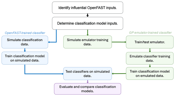
In Fig. 2, we show the workflow we used to compare two classifiers for leading-edge erosion, one trained directly on simulated data and the other trained on emulated data. In Table 5 we summarize the five datasets used in this study and their roles. We use the first dataset for the global sensitivity analysis in Sect. 2.3 to determine which of the simulation inputs have a significant effect on the sensor outputs. The statistical moments of the sensor outputs from the simulation model, which are described in Sect. 2.2.2, are used as inputs to the classifier. In order to eliminate potential bias, we perform feature ranking and selection on an independent dataset in Sect. 4.2 to rank the importance of the sensor outputs for discriminating between erosion classes and select a shorter list of predictors in order to improve classifier accuracy. In Sect. 4.3, we use the third dataset to train and test the emulator. We use the emulator to generate datasets of various sizes to evaluate the performance of the emulator-trained classifier. These datasets are shown in row 4 of Table 5. In Sect. 4.4, we use the fifth dataset as the ground truth against which to compare the emulator-trained classifiers' performance. Classifier hyperparameter tuning is done within each of the repeated 5-fold cross-validation sets. Predictions are made on the testing portion of each split, which is not seen by the model during hyperparameter tuning. The emulator-trained classification models do not train on simulation data.

Figure 2 Workflow for comparing a simulator-trained classifier with a GP-emulator-trained classifier for leading-edge-erosion classification.

Table 5 Dataset description.

4 Results

4.1 Global sensitivity analysis

The elementary effect study was carried out on the means of the five sensor output time series described in Sect. 2.2. The elementary effect analysis results show that wind shear has the least influence among the inputs tested, while wind speed has the most for each of the output QoIs. In Fig. 3 we show the normalized elementary effect plots for each sensor output. For each graph, inputs with a large μ^* have a strong, linear effect on the output, while those with a large σ interact nonlinearly with other inputs. We use a grid width of $\mathrm{\Delta }=\mathrm{1}/\mathrm{9}$ in the normalized input dimensions and r=25 trajectories for a total of 150 simulations.

Figure 3 Elementary effect plots normalized for variable magnitude on a log vs. log scale for the mean of the QoIs; (a) blade root moment (M_root), (b) blade tip acceleration (a_tip), (c) lift coefficient (C_L), (d) drag coefficient (C_D), and (e) generator power (P_gen). The same symbols are used in each subfigure for the five inputs: erosion severity, wind direction, wind speed, air density, and wind shear.

As wind shear has almost no effect on any of the output QoIs we considered, we fixed wind shear at the nominal value of 0.2. However, the limited impact of wind shear may be due to our assumption of steady-state wind conditions. Whether wind shear is influential in the turbulent case would have to be analyzed. Since μ^* is far larger for wind speed than for air density, erosion, and wind direction, this sensitivity analysis supports the need for data from across a broad range of wind speeds for training erosion detection models (Papi et al., 2020). Importantly, the rankings of air density, erosion, and wind direction vary depending on the QoI. For instance, air density impacts generator power and root moment more than other non-wind-speed inputs. Air density is known to influence turbine generator power under the same constant wind speed conditions (Golparvar et al., 2021), as it affects the power available in the wind by increasing air mass interacting with the blades. (Specifically, $P=\frac{\mathrm{1}}{\mathrm{2}}\mathit{\rho }A{v}^{\mathrm{3}}{C}_{\mathrm{p}}$, where ρ is air density, A is the swept area, v is wind velocity, and C_p is the power coefficient.) Higher air density enhances lift force generation in blades, amplifying root bending moments and increasing power output. Wind direction, which is the relative angle of the wind to the nacelle direction, is the third-most influential input for blade tip acceleration, but the fourth for every other output. In summary, the GSA study reveals that lift and drag channels are more sensitive to erosion than the other outputs we tracked (Abdallah et al., 2022; Carmona-Troyo et al., 2025; Duthé et al., 2021). As a result, we were left with a total of 9 inputs for both the simulator and emulator.

4.2 Classifier input selection

Classification results often improve when the dimension of the input space is reduced. In this subsection, we describe how we selected the inputs to the LEE classification problem from the sensor outputs. We considered 23 potential damage predictors, including wind speed, wind direction, and air density along with the mean, standard deviation, skew, and kurtosis of the QoIs listed in Table 4. To perform this reduction we use a separate OpenFAST-generated dataset and a random forest classifier to rank the potential predictors by how effectively they differentiate damage classes. To reduce bias, we repeat the predictor ranking calculation on 10 different 5-fold cross-validation splits of the simulated data. These training data include 100 samples from each erosion class obtained using a Latin hypercube design (Helton and Davis, 2003).

Figure 4 Average predictor importance score via 10 5-fold repeated cross-validation studies. Error bars represent the standard deviation of the score over the 50 train/test splits. The variables denote the mean (μ), standard deviation (σ), skew (γ), and/or kurtosis (κ) of the drag coefficient (C_D), the lift coefficient (C_L), the blade tip acceleration (a_tip), the blade root moment (M_root), and the generator power (P_gen).

We show the ranking of the damage predictors in Fig. 4. The variability in the score assigned to each predictor is relatively small, which indicates that the rank of each damage predictor is stable across model fits. The truncation limit for inclusion of a sensor output was set to be 85 % of the sum over the predictor importance of all of the inputs. This ranking is also consistent with the elementary effect sensitivity study. The most important sensor outputs include the mean and standard deviation of the drag coefficient and the mean lift coefficient. Additional selected predictors include the skewness and standard deviation of blade tip acceleration, the mean blade root moment, the standard deviation of the lift coefficient, and the mean generator power.

4.3 Emulator evaluation

4.3.1 Comparing scalar-GP emulation and PPzGP emulation

We trained and evaluated the GP emulators on the third dataset in Table 5. These simulations were generated using OpenFAST with 50 samples for each of the four eroded blade classes and 10 for the clean blade class. The training dataset varies the three environmental inputs identified by the GSA using Latin hypercube sampling over the ranges in Table 6. The erosion level in blade sections 1–6 are varied according to values given in Table 6, which we selected to ensure coverage of the stochastic erosion classes from Sect. 4.4.

Table 6 Erosion level ranges for the six blade regions and five erosion severity classes in the training data for the emulation studies.

First, we compare the training efficiency and prediction accuracy of scalar-GP emulation to that of standard parallel partial Gaussian process (PPGP) emulation, with and without the additional preprocessing step of zero-censored emulation. We test the emulators and compute 95 % confidence levels using five repeated 5-fold cross-validation sets of the OpenFAST dataset. Each split allocates 168 training points proportionally across erosion severity classes, with the remaining 42 data points reserved for testing.

Table 7 Computational cost of the standard emulators and PPEs. Values are reported as mean ±95 % confidence interval. Prediction times correspond to generating 10 000 predictions.

In Table 7 we show that the time taken to train the parallel partial emulator is 8 times less than with 8-fold scalar emulation, which is to be expected because the output vector has eight components. In Table 8 we show the normalized root mean square error (NRMSE), which, to allow for comparisons between outputs with different scales, is defined to be the root mean square error divided by the output range. The NRMSE is slightly less with the PPzGP emulator than with the standard GP emulator, which is trained to predict each output separately, except for the standard deviation of the lift coefficient, σ-C_L, and the mean of the generator power, μ-P_gen.

Table 8 Normalized root mean square error (NRMSE) for each emulator and sensor quantity selected in Fig. 4. Values are reported as mean ± 95 % confidence interval as the percentage of the output range.

In Table 9, we show the average percentage of predictions falling within the 95 % credible intervals of the PPzGP emulator for each of the eight sensor quantities. The 95 % GP credible interval contains the true function value with a rate of 0.95. If the GP model is calibrated well, under repeated sampling, the empirical coverage of the credible interval will also converge to 95 %. We observe coverage between 84 % and 95 % for the PPzGP. We attribute this to model misspecification (choice of kernel, violations of the stationarity assumption, etc.) and effects of sampling noise in the out QoI moment calculations, which we do not model directly.

Table 9 Empirical coverage in percent of the nominal 95 % credible intervals for each output.

Table 10 Paired differences between the standard GP and PPzGP emulators. Values are 95 % confidence intervals of the paired differences. Differences are computed as standard GP minus PPzGP.

In Table 10 we compare the performance of the standard GP and PPzGP emulators across the selected sensor outputs using paired 95 % confidence intervals for differences in NRMSE and empirical coverage. A positive difference in NRMSE indicates the PPzGP emulator has a lower error, while a negative difference in coverage implies the PPzGP has better coverage. These results show that PPzGP emulation provides improved uncertainty calibration for all sensor outputs while maintaining prediction accuracy comparable to the standard GP. For most outputs, the paired NRMSE confidence intervals include zero, indicating that the mean prediction errors of the two emulators are not significantly different. In contrast, the coverage intervals are mostly negative, indicating that the PPzGP intervals are generally closer to the nominal 95 % level than those of the standard GP. This suggests that incorporating physical output constraints can improve emulator uncertainty quantification without degrading mean prediction accuracy. These benefits are obtained alongside the reduced training time and storage requirements of the PPzGP formulation.

4.3.2 PPzGP emulator fitting

In Fig. 5, we compare the PPzGP emulator predictions (blue) with the simulated outputs (red), along with the associated 95 % credible intervals for four sensor outputs for one test split. For each output, the majority of true values fall within the credible intervals, indicating good emulator calibration. The generator power predictions exhibit narrow credible intervals, and the zGP ensures that the mean power does not exceed the maximum rated power of 5 MW. The statistical constraint that the blade tip acceleration standard deviation is non-negative is also enforced.

Figure 5 Predictions, ordered by simulated (true) value, and 95 % credible intervals of the PPzGP emulator model for four of eight outputs: (a) mean of drag sensor, (b) standard deviation of blade tip acceleration, (c) mean of root moment, and (d) mean of generator power.

Table 11 Wall-clock computational cost for OpenFAST simulation, emulator training, emulator prediction, and full classifier-training data generation. Prediction times are reported for generating 10 000 samples.

In Table 11, we distinguish between the cost of a single simulation, training, and generating samples with the GP emulator. All timings are wall-clock times measured on a machine with an Intel(R) Core™ Ultra 7 155H processor (3.80 GHz) and 32 GB RAM using OpenFAST-v3.5.0. Simulator timings were estimated from 25 sequential OpenFAST runs at randomly selected inputs. Emulator timings were estimated from five repeated 5-fold splits on 210 data points; prediction timings correspond to generating 10 000 emulator samples and were repeated 25 times.

Our OpenFAST simulation requires 28.4±0.3 s, whereas generating 10 000 PPzGP samples requires 0.93±0.01 s, corresponding to approximately $\mathrm{9.3}\times {\mathrm{10}}^{-\mathrm{5}}$ s per emulator sample. Thus, evaluating the fitted PPzGP is roughly 3×10⁵ times faster than running OpenFAST once. This prediction-only speedup does not include the cost of constructing the emulator. The full PPzGP workflow includes the 210 OpenFAST simulations used to train the emulator, zero-censored preprocessing for range-limited outputs, PPzGP fitting, and generation of the emulator-based classifier-training data. Using the measured OpenFAST timing, the simulator portion of this workflow costs approximately 5964 s. Zero-censored preprocessing is the most expensive part of fitting the PPzGP, but it can be sped up by preparing each output in parallel, approximately 280 s on our laptop. It takes 3.7 s for PPzGP fitting and 0.93 s to generate 10 000 samples; the full surrogate workflow requires approximately 6.2×10³ s. In contrast, directly generating 10 000 OpenFAST samples would require approximately 2.84×10⁵ s, giving a full-workflow speedup of about 46×. The prediction-only speedup and full-workflow speedup indicate that querying the fitted emulator is extremely fast, and the full workflow remains dominated by the initial OpenFAST simulations needed to train the emulator.

Figure 6 (a) Mean generator power as a function of wind speed for five levels of LEE. (b) Mean generator power as a function of wind direction for different air densities at fixed wind speed with clean blades.

In Fig. 6 we show that the PPzGP emulator captures the essential wind turbine dynamics represented by the full simulator. For this analysis, erosion is set deterministically for the values of α given in the legend with $\mathbf{e}=(\mathit{\alpha }{x}_{\mathrm{1}},\mathrm{\dots },\mathit{\alpha }{x}_{\mathrm{6}})$. In the left panel, we show generator power as a function of wind speed across five erosion severity classes. The PPzGP accurately reproduces the power curve, with higher erosion levels requiring greater wind speeds to achieve an equivalent power relative to the clean blades. The non-eroded power-curve aligns with findings from Golparvar et al. (2021), who used a GP to estimate the first and second statistical moments of generator power for a different turbine model. The PPzGP provides vector-valued predictions across multiple sensor outputs. In the right panel we demonstrate that the model captures two key physical trends: the power increases with air density and decreases when the rotor is misaligned with the wind. These relationships are consistent with prior studies (Hulsman et al., 2022) and are also evident in Fig. 6. Power loss due to erosion is proportionally highest at lower power levels, remains significant up to the rated wind speed, and disappears beyond that threshold (Campobasso et al., 2023). However, as we see in Fig. 5, model limitations exist. The prediction performance deteriorates in extreme loading conditions, particularly for high values of tip acceleration and root moment mean. These deficiencies likely stem from a lack of training data in more extreme turbine operational states.

4.4 Classification comparison

In this section we present our main results comparing two LEE classifiers using the random forest algorithm. The first, which we refer to as the simulator-trained classifier, is trained directly on the fifth dataset (OpenFAST) in Table 5. This dataset includes 120 samples from each of the five erosion severity classes where the wind speed, wind direction, and air density are varied within each class using a Latin hypercube design with ranges in Table 2. The second, which we refer to as the emulator-trained classifier, is trained using data predicted by the PPzGP emulator. For the PPzGP emulator, we compared performance using emulated datasets of several different sizes. To eliminate bias from favorable splits, we use 10 repeated 5-fold cross-validation experiments with samples balanced across the damage classes. For both classifiers, we use the same sensor outputs identified using an independent dataset in Sect. 4.2.

Within each cross-validation split, 500 simulated samples are used to train the simulation-based classifier and tune the random forest hyperparameters. Using a further 5-fold validation split within each training split to avoid overfitting, we optimize the number of learning cycles, corresponding to the number of trees in the ensemble; the maximum number of splits, which controls individual tree complexity; and the minimum leaf size, which regularizes the terminal-node size and helps limit overfitting. The emulator-trained classifier is trained using generated datasets with total sizes of 500, 1000, 5000, 10 000, and 50 000 data points. We use the emulated data to train a single model using the same hyperparameter tuning procedure. We evaluate classifier performance using accuracy, balanced accuracy, macro-F1 score, receiver operating characteristic (ROC) curves, area under the curve (AUC), and confusion matrices. Accuracy reports the overall fraction of correct predictions. The F1 score is defined by F$\mathrm{1}=\mathrm{2}\frac{pr}{p+r}$, where the precision, p, is the percentage of correct predictions out of all predictions for a given class, and the recall, r, is the percentage of correct predictions out of all true samples for a class. Balanced accuracy and macro-F1 give equal weight to each erosion class and are therefore useful when class-wise performance differs. ROC curves show the tradeoff between true-positive and false-positive rates, and the AUC summarizes class separability, with larger values indicating better performance. To compare simulator-trained and emulator-trained classifiers, paired confidence intervals are computed on model predictions from the same held-out test split from the repeated cross-validation studies.

Figure 7 Comparison of classifier performance as a function of training data source and size. Panel (a) shows macro-AUC, and panel (b) shows macro-F1 for the simulator-trained classifier and emulator-trained classifiers using 500, 1000, 5000, 10 000, and 50 000 emulated training samples. Error bars indicate 95 % confidence intervals across repeated cross-validation splits.

In Fig. 7 we show that increasing the size of the emulated training dataset improves the downstream performance of the LEE classifier. As assessed using macro-AUC and macro-F1 metrics, with 500 samples the performance of the emulator-trained classifier is worse than that of the simulator-trained classifier; with 1000 samples the performance is comparable; and with 5000, 10 000, and 50 000 samples the emulator-trained classifier outperforms the simulator-trained classifier.

Table 12 Paired differences in classifier performance between emulator-trained and simulator-trained classifiers for different emulated training-set sizes. Values are reported as mean paired difference with 95 % confidence interval. Differences are reported as points, computed as 100× the raw metric difference. Positive values indicate better performance for the emulator-trained classifier.

In Table 12 we show the paired differences between the emulator-trained and simulator-trained classifier scores for each emulated training-set size. Positive values indicate that the emulator-trained classifier performs better on the same held-out simulated test sets, while confidence intervals that do not contain zero indicate statistically meaningful differences across repeated splits. The results show a clear dependence on emulated training-set size. With only 500 emulated samples, the emulator-trained classifier performs worse than the simulator-trained classifier across all three metrics. With 1000 samples, the differences are small, indicating comparable performance. With 5000, 10 000, and 50 000 samples, the paired differences are positive for the macro-AUC, balanced accuracy, and macro-F1, showing that the larger emulator-generated datasets improve downstream classifier performance. These results suggest that the main benefit of the emulator-based workflow is not that each emulated point exactly reproduces a simulator point, but that the emulator can generate substantially larger training datasets at negligible additional computational cost, improving aggregate classifier performance.

Table 13 Per-class AUC comparison between simulator-trained and emulator-trained classifiers. The AUC difference is computed as emulator-trained minus simulator-trained, with a 95 % confidence interval for the paired difference. Differences are reported as points, computed as 100× the raw metric difference.

In Table 13 we show that the AUC performance of the best emulator-trained classifier is comparable to or slightly better than that of the simulator-trained classifier across all erosion classes. Overall, the simulator-trained classifier achieved a mean accuracy of 81.9 % with a 95 % confidence interval of [81.1 %, 82.7 %], while the emulator-trained classifier achieved a higher mean accuracy of 87.5 % with a 95 % confidence interval of [86.8 %, 88.2 %].

Table 14 Class-wise differences between models, emulator-trained minus simulator-trained. Differences are reported in points, defined as 100× the raw metric value. Each entry reports difference (p value).

A per-class comparison indicates that the emulator-trained classifier preserves performance on the clean class while improving accuracy for all eroded classes (see Table 14). The strongest improvement occurs for the 0.75 erosion class, where per-class accuracy increases by 5.6 percentage points, precision by 11.7 percentage points, and recall by 19.1 percentage points. For the fully eroded class, the emulator-trained classifier also improves per-class accuracy, precision, and recall by 3.4, 9.2, and 7.7 percentage points, respectively. The only notable tradeoff is a small decrease in recall for the mild erosion class, 0.25, despite improved precision and accuracy for that class. The largest improvements occur for the intermediate erosion classes, suggesting that the larger emulator-generated training set is especially helpful for distinguishing the more difficult class boundaries.

Figure 8 Normalized confusion matrices comparing the best emulator-trained classifier and the simulator-trained classifier. Panel (a) shows the emulator-trained classifier with 10 000 training points, and panel (b) shows the simulator-trained classifier. Rows indicate the true erosion class, columns indicate the predicted erosion class, and diagonal entries correspond to correct classifications.

The normalized confusion matrices in Fig. 8 show that both classifiers are fairly accurate, predicting the correct label with a rate greater than 0.60. Most notably the emulator-trained classifier shows slightly stronger performance for the intermediate and severe erosion classes, suggesting that the larger emulator-generated training set improves class-wise separation in the regions where misclassification is most likely.

Figure 9 One-versus-rest ROC curves for the best emulator-trained classifier and the simulator-trained classifier. Panel (a) shows the emulator-trained classifier using 10 000 emulated training samples, while panel (b) shows the simulator-trained classifier. Curves are shown for each erosion class, with shaded regions indicating variability across repeated cross-validation splits and reported AUC values given as mean ± standard deviation.

The ROC curves in Fig. 9 provide further support for the result in Fig. 8. Both classifiers exhibit high AUC values across all erosion classes, but the emulator-trained classifier provides noticeably stronger separation for the intermediate damage classes. This improvement is especially clear for classes α=0.5 and α=0.75, where the simulator-trained classifier has the lowest AUC values, indicating that the larger emulator-generated training set helps resolve the most challenging class boundaries.

While the classification accuracy improvement is modest, the computational savings are significant. Once trained the PPzGP emulator generates over 10 000 data points in less than a second. These data points are similar enough to true simulated data as to allow for comparable, or slightly improved, classifier accuracy.

Table 15 Per-class recall for the emulator-trained classifier with 10 000 generated samples and the simulator-trained classifier. Values are reported as mean recall with 95 % confidence intervals.

Because underpredicting erosion severity is more consequential than overpredicting it, in Table 15 we show the per-class recall, which is of particular importance for the most severe erosion class. One-quarter of the most severely eroded blades were classified incorrectly using the simulator-trained classifier. In contrast, the emulator-trained classifier has a recall of 83 % in the most severely eroded case. However, both of these results are high if the risk of missing a fault is severe.

Below we perform a risk-sensitive thresholding experiment. Figure 8 shows that both classifiers can underpredict severe damage, including cases where the simulator-trained classifier assigns fully eroded blades to the clean class. To mitigate this behavior, we modify the decision rule for the severe erosion class, α=1.00, by assigning a sample to the severe class whenever its severe-class probability exceeds a threshold, τ. Lowering τ increases the number of severe-damage alarms, reducing severe false negatives while increasing the false-alarm rate. We choose τ by minimizing an asymmetric confusion cost that penalizes underprediction 4 times more heavily than overprediction:

$$\begin{array}{}\text{(8)}& C_{ij}=\left\{\begin{array}{ll}\mathrm{0},& i=j,\\ \mathrm{4}|i-j|,& j<i,\\ |i-j|,& j>i,\end{array}\right.\end{array}$$

where (j<i) corresponds to underprediction of erosion severity, and (j>i) corresponds to overprediction. The average weighted confusion cost is then defined by $\stackrel{\mathrm{‾}}{C}=\frac{\mathrm{1}}{N}{\sum }_{i,j}{n}_{ij}{C}_{ij},$ where n_ij is the number of samples with true class i predicted as class j, and N is the total number of test samples. This asymmetric weighting reflects the maintenance-risk perspective that failing to detect severe erosion is more consequential than conservatively overpredicting the erosion severity.

In Fig. 10 we show that decreasing τ reduces the severe false-negative rate but increases the false-alarm rate for both classifiers, mostly for α=0.75. The weighted confusion cost is minimized at a larger threshold for the emulator-trained model, with a correspondingly lower weighted cost than the simulator-trained model.

Figure 10 Risk-sensitive threshold tuning for severe-damage detection. The severe-damage alarm threshold τ is varied for the emulator-trained classifier (a) and simulator-trained classifier (b). The dashed vertical line and star marker indicate the threshold τ^* that minimizes the weighted confusion cost for each classifier.

In Fig. 11 we show the row-normalized confusion matrices obtained using the cost-minimizing thresholds identified in Fig. 10. Compared with the default decision rule (τ=0.5), the tuned classifiers predict severe damage more often. This conservative tuning reduces the rate of severe underprediction for both the simulator-trained and emulator-trained classifiers, although it also increases overpredictions. Figure 11b shows a noticeable reduction in recall for the α=0.75 class under the tuned rule compared to Fig.8b, while the emulator-trained classifier maintains more consistent recall across the severe classes. Overall, these results show that the emulator-trained classifier can be tuned effectively to reduce high-risk severe false negatives, with a risk-reduction tradeoff comparable to that of the simulator-trained classifier.

Figure 11 Row-normalized confusion matrices for the emulator-trained classifier (a) and simulator-trained classifier (b) at the cost-minimizing severe-damage threshold τ^* in Fig. 10.

4.4.1 Robustness to sensor noise and bias

To assess whether the high classification performance in the baseline study is due to an overly clean and easily separable dataset, we performed an additional noisy-sensor classification experiment. Sensor noise was modeled by adding both a sample-level Gaussian bias and time-varying Gaussian noise to each classifier input channel. The bias standard deviation was set to 10 % of the average absolute mean sensor value, and the pointwise noise standard deviation was set to 10 % of the corresponding time series standard deviation. We kept the same sensor outputs described in Table 4. We then repeat the classifier input ranking using a noisy version of dataset 2 from Table 5 and the selection procedure from Sect. 4.2, also shown in Fig. 4, retaining μ−C_D, σ−C_D, γ−a_tip, σ−C_L, μ−C_L, μ−M_root, μ−a_tip, κ−C_D, and κ−a_tip. The emulator is then trained on a noisy version of its original training dataset. We compare the simulator-trained classifier to the emulator-trained classifier. We fit the emulator using a noisy version of dataset 3 from Table 5 and generated 10 000 data points for training the classifier. We use a noisy version of dataset 5 from Table 5 for 10 repeated 5-fold cross-validation studies.

Table 16 Class-wise recall comparison between simulator-trained and emulator-trained classifiers under noisy sensing. Average recall values are reported along with paired differences, computed as emulator-trained minus simulator-trained. Differences are reported as points, computed as 100× the raw metric difference.

In Table 16 we show that noisy sensing changes the class-wise error distribution. Compared to Table 15, all recall values are lower as expected. In comparison to the simulator-trained model on noisy data, the emulator-trained classifier has lower recall for the lowest erosion classes. However, recall improves for the intermediate classes. Recall for the most severe class remains statistically comparable between the two classifiers.

4.4.2 Classification without direct aerodynamic sensing

To further assess the dependence of the classifier on direct aerodynamic sensing, we repeat the classification study after removing the lift and drag coefficient channels. In addition to $M_{\mathrm{root}},a_{\mathrm{tip}},$ and P_gen, we consider an expanded set of structural outputs in Table 17. These channels are not directly tied to the imposed aerodynamic erosion perturbation. We calculated six additional features shown in Table 18 from the time series data and their first difference (Enríquez Zárate et al., 2022). Two features were based on frequency response using the spectrum of the time series data (Tavares et al., 2022). For a signal x(t) with power spectral density S_xx(f), the band power over a frequency interval [f₁,f₂] is

$$P_{[f_{\mathrm{1}},f_{\mathrm{2}}]}=\underset{f_{\mathrm{1}}}{\overset{f_{\mathrm{2}}}{\int }}{S}_{xx}\left(f\right)\mathrm{d}f.$$

In this study, we selected frequency bands using the range of rotor speeds observed in the data to capture energy near rotor-related frequencies. For the three-bladed turbine, both the once-per-revolution band (1P) and blade-passing band (3P) were considered.

Table 17 Additional OpenFAST output channels used in the reduced-sensing experiment. Note that we relabel RootMxb1:M_root from Table 4 as M_x,root.

Table 18 Additional time series descriptors used in the reduced-sensing experiment.

We repeated the predictor selection process from Sect. 4.2 four times, ranking and selecting the top 14 quantities from an initial list of 108: $\mathit{\gamma }-a_{x,\mathrm{tip}}$, $\mathit{\mu }-M_{x,\mathrm{root}}$, $\mathit{\mu }-F_{y,\mathrm{root}}$, ${\mathit{\rho }}_{\mathrm{1}}-a_{z,\mathrm{tip}}$, ${\mathrm{BP}}_{\mathrm{3}\mathrm{P}}-M_{z,\mathrm{root}}$, $\mathrm{NFD}-a_{z,\mathrm{tip}}$, ${\mathit{\rho }}_{\mathrm{1}}-M_{y,\mathrm{tower}}$, ${\mathit{\rho }}_{\mathrm{1}}-M_{z,\mathrm{shaft}}$, $\mathit{\kappa }-M_{z,\mathrm{shaft}}$, ${\mathit{\rho }}_{\mathrm{1}}-M_{y,\mathrm{shaft}}$, ${\mathrm{BP}}_{\mathrm{3}\mathrm{P}}-M_{y,\mathrm{tower}}$, ${\mathit{\rho }}_{\mathrm{1}}-M_{x,\mathrm{tower}}$, $\mathit{\kappa }-M_{z,\mathrm{root}}$, and $\mathit{\kappa }-a_{x,\mathrm{tip}}$. The two highest-ranked predictors, $\mathit{\gamma }-a_{x,\mathrm{tip}}$ and $\mathit{\mu }-M_{x,\mathrm{root}}$, were also ranked highly in the primary study, suggesting their importance even without the aerodynamic sensor channels.

We train the emulator on a separate dataset with 210 samples and then use 10 repeated 5-fold cross-validations and inner-loop hyperparameter tuning to compare the simulator-trained and emulator-trained classifiers with dataset 5 from Table 5. In this experiment, we used the emulator to generate a dataset of 50 000 samples.

Figure 12 Confusion matrices for classification using non-aerodynamic sensor channels with emulator-trained classifier (a) and simulator-trained classifier (b).

Table 19 Comparison of simulator-trained and emulator-trained classifiers under the reduced-sensing experiment. Values are reported as mean classifier score with standard deviation. Paired differences are computed as emulator-trained minus simulator-trained and are reported with 95 % confidence intervals. Differences are reported as points, computed as 100× the raw metric difference.

In Fig. 12 we show that, after removing the aerodynamic lift and drag channels, classifier performance decreases substantially relative to the full-sensing case shown in Fig. 8, confirming that with less access to aerodynamics-based sensors the classification problem is more difficult. However, the simulator-trained and emulator-trained classifiers have comparable class-wise behavior. Nonetheless, the confusion matrices are dominated by their diagonal entries, indicating that misclassifications typically occur between adjacent erosion classes rather than between widely separated damage states. The severe erosion class remains identifiable, with both classifiers correctly classifying 73 % of α=1.00 samples. Consistent with the confusion matrices, in Table 19 we observe nearly identical balanced accuracy and macro-F1 values for the two classifiers, indicating that the emulator-trained classifier remains statistically comparable to the simulator-trained classifier in the case of no direct aerodynamic sensors.

5 Discussion

In this paper we provide a proof-of-concept study for the use of wind turbine emulators to generate data for SHM. Even though turbulent inflow makes distinguishing between different levels of LEE more difficult, we believe it is possible to extend the proposed modeling framework to more realistic operating conditions, including turbulent flow, controller transitions, and yaw adjustments. The OpenFAST turbulence model is parametrized by moments such as average wind speed and the mean and covariance of turbulence intensity, which could be used as inputs to an emulator. More complex operating conditions would require much longer OpenFAST simulations (on the order of tens of minutes rather than seconds) to extract reliable statistical features from time series information. In steady-state simulations, we achieved good results with a comparatively small dataset. However, in order to fit a GP on complex simulations, more simulations will likely be required to achieve high emulator accuracy, which may require different emulator fitting strategies (Clark and Clark, 2022). However, in the case of long simulation runs, the speedup from using an emulator would be even greater than in the current study.

The main motivation for development of the emulator is to reduce the computational cost of running a digital twin for monitoring LEE. We envisage that the PPzGP emulator in this paper would serve as the kernel of a probabilistic, graph-based digital twin for tracking damage progression over time (Kapteyn et al., 2021). Areas in which this study could be extended include accounting for how real turbine monitoring data are affected by sensor noise, controller behavior, atmospheric variability, and maintenance history. Further, in this work we do not track erosion progression over time. Closing the gap would require additional development of the surrogate model to include effects like turbulence and validation of an improved surrogate model by comparison with field data (SCADA data and blade inspections) (Duthé et al., 2021; Visbech et al., 2023). Secondly, our erosion proxy does not capture the nonlinear effects on aerodynamic lift and drag polar as a function of erosion damage. Thus, while the emulator fitting results are promising, they should be interpreted within the context of our heuristic erosion model. Future work should incorporate more realistic nonlinear effects on erosion dynamics.

6 Conclusions

This study compares LEE classification using both a full physical simulator-trained random forest classifier and one trained by sampling a computationally efficient emulator. We show that these two damage classifiers provide similar classification results, as evaluated through a variety of ML metrics at predicting levels of LEE damage on WT blades in three proof-of-concept studies. The main contribution of this work is the use of the PPzGP emulator as a computationally efficient surrogate model for enabling damage classification tasks. The PPzGP can be trained on a relatively small set of full physical simulations. It can be adapted to handle arbitrarily large numbers of output QoIs without increasing the overall training cost, and the zero-censored emulator incorporates physical turbine constraints. Taken together, the advantages of this emulation-based framework lead to a reduction in computational cost and could be integrated into real-time SHM systems, such as those that comprise a digital twin.