
the Creative Commons Attribution 4.0 License.
the Creative Commons Attribution 4.0 License.
 | 18 Sep 2026
Assessing the accuracy of a 3-year high-resolution mesoscale wind farm wake simulation with lidar and satellite radar data
Alexandros Palatos-Plexidas

Simone Gremmo
Jeroen van Beeck
Lesley De Cruz
Wim Munters
The rapid expansion of wind farm installations in the North Sea results in an increased need for understanding their influence on the local atmosphere, as well as the interactions between them. Wind farm operation and power production are affected by wakes produced both within and upstream of the wind farms. Accurately estimating these impacts requires robust mesoscale atmospheric modeling capable of capturing extended wind speed deficits and their dependence on atmospheric stability. This study presents a 3-year-long mesoscale analysis using the Weather Research and Forecasting (WRF) model at a horizontal resolution of 1 km, a comparatively long and high-resolution configuration within the context of offshore wake research. The simulations are evaluated against four lidars located in the Southern Bight of the North Sea in the vicinity of the 3.7 GW Belgian–Dutch offshore wind farm cluster, providing an extensive observational basis that covers upstream, intra-farm, and downstream flow conditions. Coupling the mesoscale atmospheric model with the Fitch wind farm parameterization scheme improves simulation accuracy, particularly in regions frequently affected by wake effects. An evaluation across different atmospheric boundary layer stability regimes shows that the model performs best under less extreme stability, while a detailed assessment of upstream, intra-cluster, and downstream wake characteristics highlights the added value of the Fitch scheme for multi-year offshore applications. Finally, synthetic aperture radar images from selected wake events are compared with the model output, demonstrating that the wind farm parameterization scheme effectively captures the larger-scale structure and wind speed deficit of the wind farm wake at the analyzed timestamps. Together, these results provide one comprehensive long-term evaluation of offshore wake behavior in a dense wind farm cluster, helping to address the current gap in mesoscale wake studies.
- Article
(10887 KB) - Full-text XML
- BibTeX
- EndNote


In recent years, wind energy has become one of the most promising electricity generation technologies for a sustainable energy system. Especially offshore, wind farms are growing in size and number, resulting in gigawatt-scale clusters being installed in each other's vicinity. Therefore, it is important to quantify the effects of wind farms in terms of both how their interaction impacts operation and energy production and their local influence on the atmosphere. These effects vary based on the predominant atmospheric conditions and wind characteristics.
One of the most pertinent tasks is the understanding and quantification of wake effects produced by wind farms. Wakes exert a substantial influence on downstream wind turbines, as they lead to decreased wind speeds and increased turbulence that affect both the power production and the fatigue of the wind turbine (Stanley et al., 2022; Jézéquel et al., 2024). Crucially, wakes are the dominant driver of power losses in offshore wind farms, reducing power extraction of the order of 10 % to 20 % compared to lone-standing turbines (Lee and Fields, 2021). Furthermore, especially for large wind farms, individual turbine wakes merge into wind farm wakes that have been shown to persist several tens of kilometers downstream of the wind farm, depending on the atmospheric conditions (Ali et al., 2023). As a result, offshore wind farms are affected by current and future neighboring farms, and reducing uncertainties in these interactions is becoming increasingly important for the efficient development of offshore wind energy.
High-fidelity simulations like large-eddy simulations (LES) can provide useful insights into the interaction between wind turbines and the atmospheric boundary layer (ABL), with different approaches for wind turbine representation being developed (Sorensen and Shen, 2002; Stevens et al., 2018; Stipa et al., 2024). However, computational cost for high-resolution LES remains very high, rendering them impractical for simulating large wind farm clusters over long periods. In addition, performing LES under real atmospheric conditions increases the computational cost further as proper coupling with a mesoscale model is required (Muñoz-Esparza et al., 2014; Haupt et al., 2023; Kale et al., 2023). As a result, mesoscale numerical weather prediction (NWP) models remain the most cost-effective state-of-the-art tool to assess atmospheric conditions spanning a wide geographic area and a prolonged period. NWP models typically operate on horizontal grid spacings of 1 to 3 km, necessitating the use of different parameterization schemes to capture the effects of subgrid-scale physics such as convection, hydrometeor microphysics, radiation, surface interactions, and turbulence. Over the past years, many NWP models have also included parameterization schemes to account for the influence of the wind turbines within the ABL. An extensive description of these wind farm parameterization (WFP) schemes in NWP models can be found in the work of Fischereit et al. (2022a).
In particular, although several alternatives have been developed (Volker et al., 2015; Ma et al., 2022a), the most widely used WFP scheme in NWP models is the method proposed by Fitch et al. (2012). Even though the scheme has significant limitations, e.g., in the turbulence kinetic energy (TKE) representation (Archer et al., 2020), the freestream wind estimation (Vollmer et al., 2024), and the inclusion of subgrid-scale wakes (Ma et al., 2022b), the original implementation has been shown to agree reasonably well with high-fidelity simulations (Archer et al., 2020; Peña et al., 2022; Fischereit et al., 2022b; García-Santiago et al., 2024), field measurements (Larsén and Fischereit, 2021; Ali et al., 2023; Fischereit et al., 2024), and turbine production data (Lee and Lundquist, 2017; Santoni et al., 2020). Nevertheless, further validation studies over extended time periods are needed to reduce uncertainties in quantifying wind farm wakes and the resulting inter-farm interactions (Fischereit et al., 2022a).
The vast majority of WFP studies utilize the Weather Research and Forecast (WRF) model (Skamarock et al., 2019). WRF is an open-source and widely used NWP model able to simulate complex atmospheric phenomena and extreme events (Larsén et al., 2019; Shenoy et al., 2021; Müller et al., 2024). It has been used in a variety of studies that estimate the influence of wind farm effects (e.g., Pryor et al., 2019, 2020; García-Santiago et al., 2023), including analyses of wind farm effects under different ABL stability conditions (Cañadillas et al., 2020; Rosencrans et al., 2024; Palatos-Plexidas et al., 2024). In addition, specific events like extreme winds (Pryor and Barthelmie, 2021), storms (Ivanova et al., 2025), and low-level jets (Vanderwende et al., 2015; Quint et al., 2025; Olsen et al., 2025) are well reproduced by WRF at different locations across the globe. Although there are a few studies that simulate the wind farm effects using mesoscale models at 1 km or sub-kilometer scales under real atmospheric conditions (Gomez et al., 2024), long-term high-resolution mesoscale simulations and validations remain largely absent from the literature.
The current work presents an assessment of model performance and analysis of wake effects from a 3-year-long high-resolution (1 km) WRF simulation of the Southern Bight of the North Sea, with a specific focus on the 3.7 GW Belgian–Dutch wind farm cluster. This cluster consists of several high-density wind farms installed next to each other, making it the largest offshore cluster operational today, hence resulting in a prime test case for studying wind farm wakes. Extending the analysis over 3 years enables a comprehensive characterization of seasonal patterns and temporal variability.
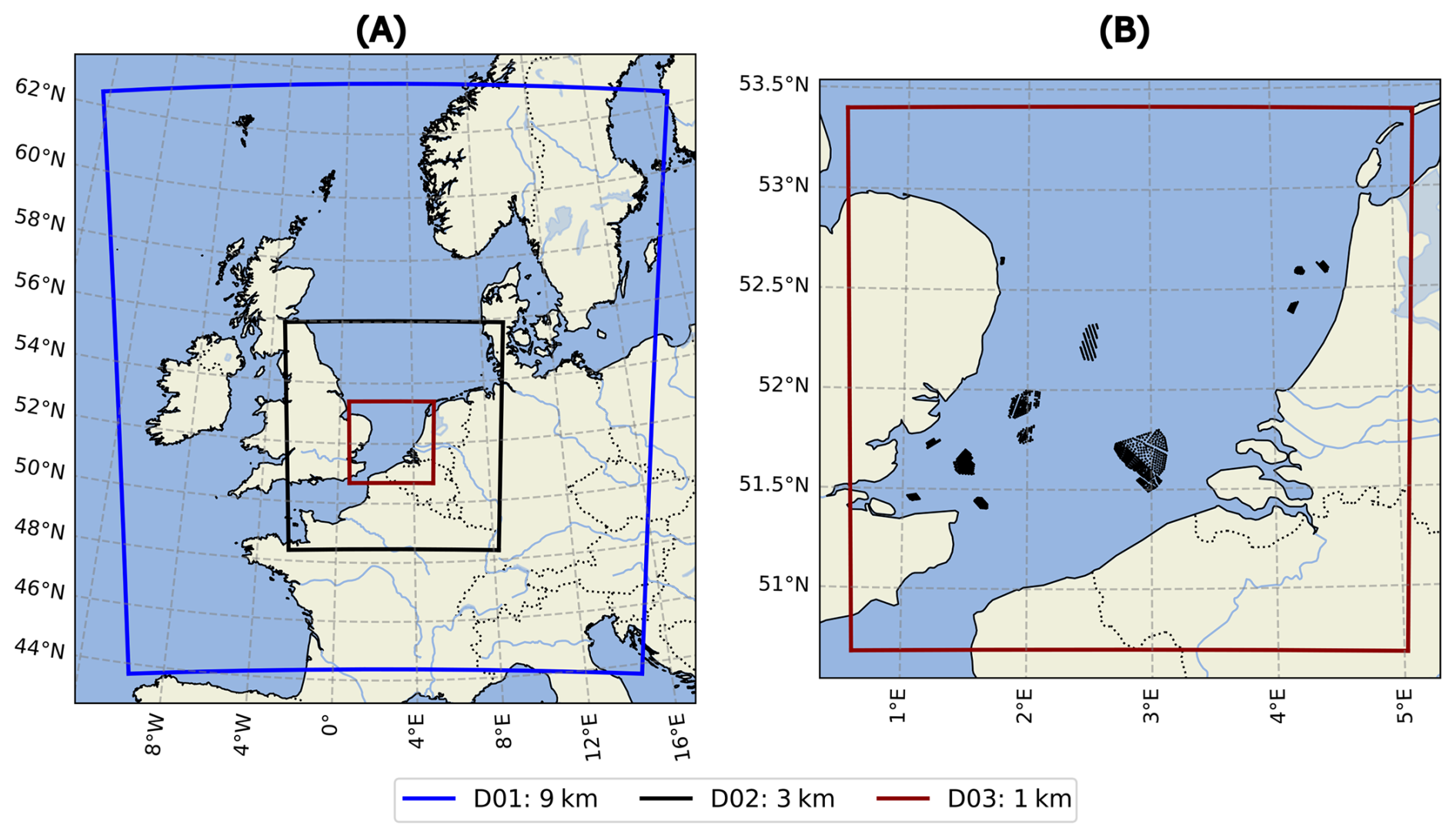
Figure 1(A) Map of the three nested domains used for the WRF simulations, with a horizontal resolution of 9 km (D01, blue box), 3 km (D02, black box), and 1 km (D03, red box). (B) Zoomed-in view of the high-resolution innermost domain (D03), including the simulated wind turbines (black dots).
This study is driven by two primary objectives that address notable gaps in current offshore wake research. The purpose of this study is not to validate the Fitch parameterization in isolation, but rather to assess the long-term predictive performance of the full WRF–Fitch modeling system for offshore wake dynamics in an operationally relevant environment. First, we assess the 3-year WRF–Fitch simulation performance using lidar measurements positioned both within and around the Belgian–Dutch cluster, enabling an evaluation of model performance under varying ABL stability regimes. This is particularly relevant given that long-term wake validations at 1 km resolution (assessed under different stability regimes) remain rare, especially in densely built offshore environments. The strategic placement of the lidar probes allows us to assess how the model represents inflow conditions, intra-cluster wake dynamics, and downstream recovery for different wind directions and wind speed regimes, and the availability of four lidars spanning upstream, downstream, and intra-farm positions provides a uniquely comprehensive observational basis for this evaluation. Second, we evaluate the performance of WRF for a set of specific wake events by comparing the simulated wake signatures with satellite-retrieved wind fields. This dual comparison, quantitative through lidar transects and qualitative through two-dimensional SAR wake structures, provides a robust, multi-sensor estimation of wake deficits, blockage effects, and model skill. Together, these objectives provide a comprehensive long-term evaluation of offshore wake behavior in a high-density wind farm cluster.
The remainder of the study is structured as follows. Section 2 outlines the methodology, including the WRF model setup, the classification of ABL stability, the measurement datasets used, and the definitions of performance metrics. Section 3 highlights the simulation results, including the overall atmospheric conditions and model performance assessed against lidar data under varying stability conditions, wind speed magnitudes, and specific events. An additional analysis of upstream, intra-farm, and downstream wake characteristics based on WRF simulations is also presented. Finally, Sect. 4 summarizes the main findings of this study.
This section outlines the methodology used to create and analyze the high-resolution dataset. First, the configuration of the WRF model is described. Next, the definition and the classification of atmospheric stability regimes are introduced. Finally, the lidar observations and the SAR images used for model performance assessment are presented, followed by the evaluation metrics applied in this study.
Nakanishi and Niino (2006)Monin and Obukhov (1954)Mukul Tewari et al. (2004)Kain (2004)Hong et al. (2004)Iacono et al. (2008)Table 1Physics parameterization schemes selected for this study in WRF, along with their associated references.

2.1 WRF model setup
Simulations were performed with version 4.5.2 of the WRF model (Skamarock et al., 2019) over a period of 3 years: 2021, 2022, and 2023. The initial and boundary conditions are derived from 30 km spatial resolution ERA5 hourly reanalysis data (Hersbach et al., 2020). Three nested square domains are employed with grid resolutions of 9, 3, and 1 km, respectively, as depicted in Fig. 1. Furthermore, one-way nesting is applied to prevent any potential noise generated within the innermost domain from propagating into the parent domains. In the vertical direction, 80 non-equidistant levels are used up to 50 hPa, while the first 30 levels are densely distributed starting from approximately 5 m up to 320 m height, with an average vertical resolution of 11 m. Adaptive time stepping is used with a target Courant–Friedrichs–Lewy number of 0.84 and 0.6 for the horizontal and vertical directions, respectively. In addition, vertical velocity damping is enabled to ensure robustness and stability during the multi-year runs using a Rayleigh damping layer with a depth equal to 5000 m from the model top and a damping coefficient of 0.15 m s−2. The results of the high-resolution domain D03 are processed every 10 min for comparison to lidar data. The model physics configuration is based on the New European Wind Atlas (NEWA) setup (Hahmann et al., 2020; Dörenkämper et al., 2020) and is presented in Table 1. The cumulus scheme is activated only at the outermost domain of 9 km resolution. Regarding the planetary boundary layer (PBL) turbulence modeling, the MYNN 2.5 (Nakanishi and Niino, 2006) scheme is used, as it is the only scheme available in WRF v4.5.2 that allows for the advection of TKE produced by the WFP as explained below. Note that, rather than performing a specific sensitivity study to optimize model skill for the location of interest, a single WRF configuration, close to the well-known NEWA setup, is chosen in order to evaluate a typical out-of-the-box performance of the model against measurements.
Wind farm parameterization
For this study, the WFP scheme proposed by Fitch et al. (2012) is used. The influence of turbines on the atmosphere is described by imposing a momentum sink in the mean flow, which enables the conversion of a fraction of the kinetic energy (KE) into electricity, while the remaining KE is transformed into TKE. The WRF model is executed with and without wind farm parameterization activated (hereafter WF and NWF, respectively) within a single model run, using two identical D03 domains, to isolate wake effects. The study focuses on the investigation of the Belgian–Dutch cluster; however, nearby offshore wind farms in the Southern Bight of the North Sea, i.e., in the UK and in the Netherlands, are included in the simulations. The locations of all the wind turbines included in the simulations are obtained from the study of Hoeser et al. (2022). The wind farms are depicted in Fig. 1b, and they are exclusively simulated on the highest-resolution domain. The main characteristics of the wind turbines used are presented in Table A1 in the Appendix. The principal equations for describing the influence of the wind farms on the mean flow in a discrete Cartesian computational cell (i, j, and k) are defined as
These equations describe the change in horizontal wind speed , the TKE enhancement due to wind turbines, and the wind power production P, where zk defines the height at model level k, and Aijk is the cross-sectional rotor area of one wind turbine between the height levels k and k+1. Furthermore, is the number of turbines located within the computational cell (i,j). The thrust coefficient CT and power coefficient CP depend on the wind turbine type and are obtained from a mix of public and confidential data. The TKE coefficient is defined as , with α=1 in the original Fitch implementation, driven by the idea that momentum lost by the mean flow, which is not converted to electrical power, is transformed into turbulence. However, it was found that this can lead to a significant overestimation of the TKE compared to high-fidelity simulations (Archer et al., 2020). Although there remains significant debate over the appropriate value of α (Larsén and Fischereit, 2021; García-Santiago et al., 2024), this study uses the current default value in WRF; i.e., α=0.25. A 6-month sensitivity analysis using α=0, α=0.25, and α=1 is presented in Appendix A2 (Figs. A1 and A2), indicating that no single α value consistently outperforms the others, given the considered time period and locations. Last, ec in Eqs. (1) and (2) is the energy correction factor that ensures that the vertically distributed extraction matches the turbine power curve at hub height (adapted from the WRF source code). The wind speed deficit due to the wind turbine influence is defined as the normalized difference between the unperturbed and the wind-farm-affected wind speed; i.e., .
For simplicity, we consider the area-averaged momentum flux deficit:
where ρ0 is the density of the atmosphere near hub height, assumed constant and equal to 1.225 kgm−3, S is the area of interest (e.g., the Belgian–Dutch cluster area), and Nc is the number of computational cells within this area.
The thrust force for each wind turbine is also computed:
where AT is the area swept by the rotor blades, estimated using the rotor diameter of each turbine, and Uhub is the hub-height wind speed within a grid cell when the Fitch scheme is activated (WF).
2.2 Atmospheric boundary layer stability
The stability conditions in the lower layers of the ABL can be assessed by analyzing temperature, wind speed, and surface heat fluxes (Stull, 2015). These variables are closely associated with atmospheric turbulence and the resulting wake mixing. In this work, the atmospheric stability is characterized by the value of Obukhov length L (Monin and Obukhov, 1954), as retrieved from WRF via the inverse L (RMOL) variable. Obukhov length governs how shear and buoyancy contribute to the production and dissipation of TKE:
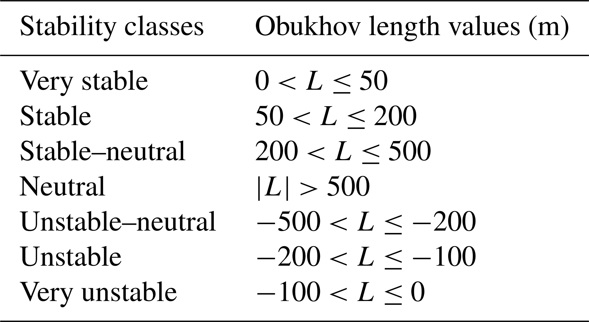
where u∗ is the friction velocity, is the mean virtual potential temperature at the first model level above the surface (approximately at 5 m), κ=0.41 is the von Kármán constant, g = 9.81 m s−2 is the gravitational acceleration, and is the surface virtual potential heat flux. Stable conditions are present when L>0, when shear production and buoyancy destruction counteract, leading to limited turbulence and intermittency. In contrast, when L<0, buoyancy enhances turbulence, resulting in stronger vertical motion and mixing. In neutral conditions, when , buoyancy has a negligible effect and turbulence is driven solely by shear. Besides the main stable, unstable, and neutral conditions, four additional ABL stratification categories, as defined in Table 2, are considered in the analysis, seeking to deliver a more comprehensive representation of the stability conditions. This approach is similar to the work of Gryning et al. (2007) and has been implemented in the studies of Olsen et al. (2022) and Palatos-Plexidas et al. (2024).
Table 2Atmospheric stability classes. Obukhov length L values are assessed from WRF simulations (Eq. 6), and seven classes are selected, adapted from the work of Gryning et al. (2007).
2.3 Offshore observations
There are two sources of observations used in this work, and they are presented in this section. Initially, lidar profile measurements are employed to assess model performance throughout the entire analysis period. Subsequently, synthetic aperture radar (SAR) data from the Southern Bight of the North Sea are utilized to compare and validate the model-assessed wakes at specific events.
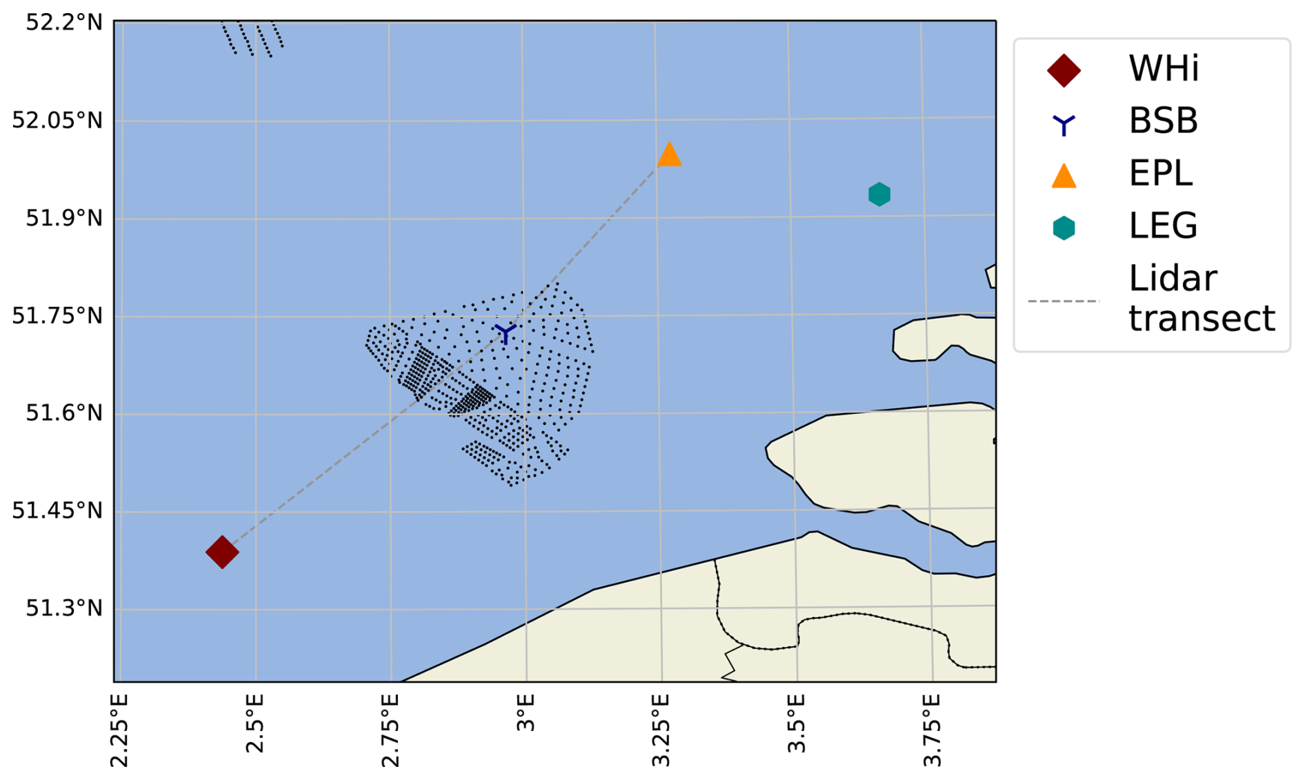
Figure 2Measurement locations in the domain of interest. The black dots indicate turbine locations included in the WRF simulations.
Table 3Description of the lidars used in this study. Data availability is expressed as the percentage of time each lidar was operational relative to the full simulation period (2021–2023). Timestamps of missing data are also accounted for in the table.

∗ Data availability refers to the timestamps for which wind speed and wind direction measurements overlap. The table also presents the final number of timestamps retained for analysis after applying the filtering procedure described in Sect. 2.3.3.
2.3.1 Lidars
Model performance is evaluated against 10 min averaged wind speed and wind direction measurements from four vertical profiling lidars located in the Southern Bight of the North Sea, close to the Belgian–Dutch wind farm cluster. As discussed below, considering the wind roses at this site, the locations of the lidars (see Fig. 2) provide a unique opportunity for assessing wake effects. Details on their location and the operation period during the simulation time window are described in Table 3. The following lidars are considered:
-
WHi. The Westhinder (WHi) lidar is a ZX 300M installed on the Westhinder (MP7) survey platform located approximately 40 km southwest of the Belgian–Dutch cluster, close to the French border in Belgium. The lidar was installed in August 2021 and is operated by the von Karman Institute for Fluid Dynamics (Glabeke et al., 2023). In this study, we utilize data from the campaign between 4 August 2021 and 18 July 2022. The lidar measures at 11 different heights, i.e., 34.5, 44.5, 62.5, 79.5, 104.5, 124.5, 149.5, 174.5, 224.5, 274.5, and 324.5 m TAW. Measurement heights are in meters above the Tweede Algemene Waterpassing (m TAW), implying that the average sea level at low tide in Ostend (Belgium) is used as the zero level. This value lies 2.3 m below mean sea level.
-
EPL and LEG. Northeast of the cluster, two more lidars are installed on the Europlatform (EPL) and Lichteiland Goeree (LEG) platforms, respectively. Data are provided by the Wind Energy Research Group of TNO, which operates the lidars (Verhoef et al., 2020; Bergman et al., 2022). LEG features a Leosphere WindCube lidar v2.1 providing measurements at eight heights, i.e., 62, 90, 115, 140, 165, 190, 215, and 240 m above mean sea level. EPL is equipped with a ZX 300M lidar (Verhoef et al., 2020), with data provided at 63, 91, 116, 141, 166, 191, 216, 241, 266, and 291
-
BSB. Inside the cluster, data from the ZX 300M lidar installed at the TenneT platform Borssele B (BSB) and operated by the KNMI are used (Knoop and de Jong, 2023), with measurements at 11 heights, i.e., 59, 83, 108, 117, 139, 164, 190, 201, 224, 244, and 294
Considering the prevalence of southwesterly and, to a lesser extent, northeasterly wind directions at this site (see Fig. 4), the combination of WHi, BSB, EPL, and LEG provides a suitable alignment to include a freestream, intra-cluster wake and far-wake observation for these wind directions. All lidar observations come in the form of 10 min averages. Both lidar measurements and model output are interpolated to a reference hub height of 107 m above ground level, corresponding to the hub height of many wind turbines within the domain of interest.
2.3.2 SAR data
The SAR data used in this study were retrieved by the Sentinel-1 European Space Agency mission. More specifically, there are two satellites, Sentinel-1A (2014–present) and Sentinel-1B (2016–2021), equipped with C-band synthetic aperture radar (SAR) instruments operating at 5.405 GHz, and both satellites follow a sun-synchronous polar orbit at an altitude of 693 km (Hasager et al., 2024). Focusing on the area of interest, including the Belgian–Dutch wind farm cluster in the Southern Bight of the North Sea, as well as additional upstream and downstream areas to study potential wake structures, the analyzed time instances occur approximately at 06:00 UTC every 12 d and at 17:40 UTC every 6 d, respectively (Sentinel-1A, 2021–2023). The operation of Sentinel-1B during 2021 provided an additional set of overpasses at around 17:32 UTC every 6 d. This corresponds to approximately 8 to 10 SAR snapshots per month over the area of interest during the analyzed period. The wind speed at 10 m height is then estimated by applying the CMOD5N geophysical model function (Hersbach et al., 2007), as also explained in the work of Siedersleben et al. (2020). This indirect-retrieval method assumes that radar backscatter from the sea surface, which reflects centimeter-scale waves generated by instantaneous wind stress, can be converted into wind speed at 10 m height (Ahsbahs et al., 2017, 2018). The wind fields are provided at a 500 m pixel resolution through the Global Wind Atlas Science Portal of the Danish Technical University (DTU) Wind Energy Department (https://science.globalwindatlas.info/#/map/satwinds, last access: 30 July 2025).
2.3.3 Data filtering
Two different types of filtering are used for the lidar measurements and the SAR data, respectively. For the lidars, we apply a threshold and discard wind speed values outside the range of [0.5,70] m s−1. The lower bound was set to discard very low wind speeds in which the wind direction becomes ill-defined. A similar approach was taken by Pentikäinen et al. (2023). It was verified that this bound does not significantly impact wind speed validation results. The upper bound discards spuriously high measurements. The resulting interval retains relevant wind speed values for wind energy purposes, including wind speeds below cut-in and above cut-out. The same thresholds are applied to the WRF wind speeds in both the NWF and the WF simulations (discarding approximately 0.3 % of the WRF timestamps). To avoid 180° wind direction ambiguity in the lidar data, we exclude instances exhibiting abrupt directional shifts greater than 120°, as these are considered non-physical. Although such outliers could alternatively be corrected using nearby observational sources or the WRF output, we opt to discard them entirely to ensure a more robust and reliable observational dataset. This filtering results in an additional data removal of approximately 1 %–2 % of the total values presented in Table 3, depending on the location. We then use the common timestamps of both filtered lidar and WRF datasets for evaluating both wind speed and wind direction.
The SAR data are polluted by wind turbines and ships in the area of interest, creating local outliers in the retrieved wind fields. In this case, we use a Hampel filter to detect the outlier values (Hampel, 1971). This method detects localized outliers of a series of data using the median absolute deviation (MAD) in a sliding window of size Wi. The median value mi is computed across the sliding window, and the MAD is defined as , where xj is the value in the sliding window Wi. The MAD is scaled to be comparable to the standard deviation for Gaussian data as . A point xi is considered an outlier if . In this study, the Hampel filter is applied across the transect that connects WHi, BSB, and EPL locations (see Fig. 19). To detect outliers, we use a sliding window Wi=3 and set nσ=3 to prevent excessive outlier detection and ensure robustness without over-filtering the data.
2.3.4 Evaluation metrics
Different evaluation metrics are used to provide a comprehensive understanding of model performance. More specifically, the bias, the centered root mean squared error (cRMSE), the Pearson correlation coefficient (r), and the Earth Mover's Distance (EMD) are computed for the wind speed and the wind direction. The mathematical definitions of these metrics are provided in Appendix A1. The same metrics have been employed in several studies to evaluate model performance in calculating wind fields (Rosencrans et al., 2024; Olsen et al., 2025).
The bias score measures the systematic error between the simulations and the observations, indicating a consistent overestimation (positive bias) or underestimation (negative bias). The cRMSE is used to quantify the average error magnitude between the model and the lidars, emphasizing the variability around the mean value. The EMD evaluates the similarity between two distributions by calculating the minimum cost required to transform one distribution into another, thereby facilitating the comparison of the overall shape and distribution of predicted and observed wind speed and wind direction data. The Pearson correlation coefficient (r) measures the linear relationship between predicted and observed values. While bias, cRMSE, and EMD values closest to zero indicate better model performance, the Pearson correlation coefficient (r) ranges from −1 to 1, with values closer to 1 signifying a stronger direct linear relationship between the model and the lidar measurements. To compute means of the wind direction, the circular mean is applied (Mardia and Jupp, 2009). The cRMSE equation for circular variables (Eq. A6) has been adopted from the study of Rosencrans et al. (2024). Instead of the Pearson correlation for linear values, the circular–circular correlation ρ is used (Mardia and Jupp, 2009). All metrics are computed using the built-in functions of the NumPy (Harris et al., 2020) and SciPy (Virtanen et al., 2020) Python packages. Furthermore, the wasserstein_circle function from the Python Optimal Transport (Flamary et al., 2021) package is used to calculate the EMD for the wind direction.
Last, for the SAR transects, we compute the mean absolute error, , where n is the number of points across the upstream, intra-farm, and downstream regions of each transect (70 points in total after regridding the SAR and WRF data). In addition, for the same time instances, we evaluate the point-wise absolute error, , using the lidar observations as reference.
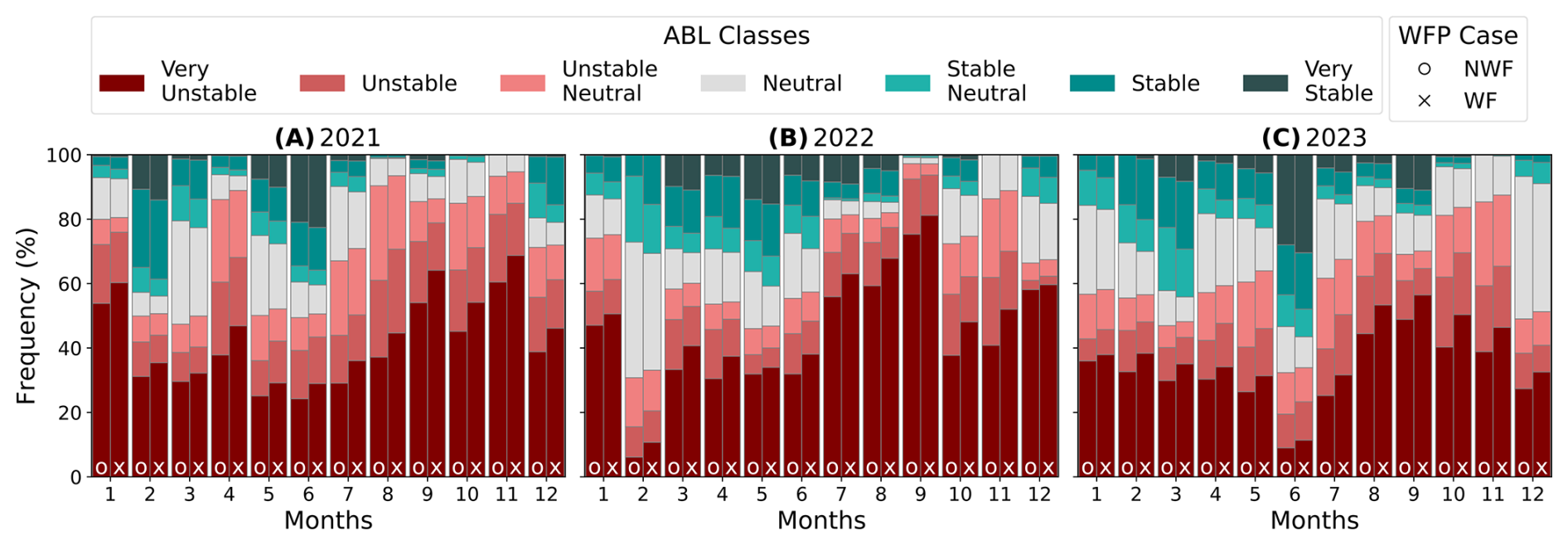
Figure 3ABL classification based on the WRF-estimated L values at the BSB location over the 3-year simulation period. The stability classes are described in Table 2. On the y axis, the frequency of each ABL condition is depicted, and on the x axis, the months of each year, from 1 (January) to 12 (December), are shown. Bars marked with “o” and “x” correspond to the NWF and WF simulations, respectively.
This section discusses the simulation results and compares them to observations. First, Sect. 3.1 investigates the atmospheric conditions during the simulation period, focusing on dominant stability regimes and wind roses. Next, Sect. 3.2 compares model results to lidar observations. In addition to the validation of the full 3-year dataset, the impact of stability on model performance is quantified. Further, wind fields along the lidar transect (see Fig. 2) are analyzed to focus more specifically on wind speed deficits (Sect. 3.2.3) and blockage (Sect. 3.2.4). Finally, Sect. 3.3 presents a comparison between WRF and SAR data for four specific events.
3.1 Atmospheric conditions
Two main atmospheric characteristics are considered for the investigation, the Obukhov length (Eq. 6 and Table 2) and the wind fields presented as wind roses, assessed at the four lidar locations. All results presented in this study use wind speed and direction rotated to Earth-fixed coordinates. Furthermore, only the horizontal wind speeds (hereafter referred to as wind speeds) are analyzed both in the measurements and in the models. Figure 3 illustrates the monthly-averaged L distributions for the years 2021 (Fig. 3a), 2022 (Fig. 3b), and 2023 (Fig. 3c). The values of L are calculated using WRF at the BSB lidar probe, for both the NWF (left bars indicated with “o”) and the WF (right bars indicated with “x”) simulations. Despite the intra-annual variability in ABL stratification, the monthly L distributions indicate that very unstable conditions prevail over the 3-year-long analysis. Peaks of the very unstable atmospheric conditions predominantly occur in January, as well as during late summer and autumn.
Stable and very stable atmospheric conditions are primarily observed from late winter through early summer, while their occurrence is significantly reduced during autumn. Specifically, June 2021, May 2022, and June 2023 exhibit notably high frequencies of stable and very stable atmospheric conditions. Furthermore, a significant number of neutral cases is also observed. The frequency of neutral or near-neutral conditions is associated with strong winds, which enhances the importance of shear effects over buoyancy. For example, in February 2022, severe storms occurred (Ivanova et al., 2025), resulting in a higher frequency of neutral events over the Southern Bight of the North Sea.
Overall, the predominance of unstable to very unstable events has been highlighted in several studies over the past decade. For example, Archer et al. (2016) demonstrated that the marine ABL along the US northeastern coast was mostly unstable during a 2003–2011 measurement campaign. Similar conclusions for the North Sea have been reported in recent WRF-based studies (Porchetta et al., 2024; Palatos-Plexidas et al., 2024). However, it is important to note that ABL stability strongly depends on the region and period of interest. For instance, Rosencrans et al. (2024) found an almost equal mix of unstable and stable conditions, with relatively few neutral cases, in the Rhode Island–Massachusetts area based on WRF simulations from September 2019 to September 2020.
In addition to the intra-annual stability distributions in the BSB location, the influence of the wind turbines on the ABL stratification should be addressed. The inclusion of wind turbines affects the intra-farm ABL stratification, resulting in an increase of 5 % to 15 % of the very unstable events during the 3-year period. In addition, an increase in very stable instances is observed, while neutral and close-to-neutral cases are slightly reduced. The increase in very unstable and very stable cases may be attributed to the wind-farm-induced wake, which leads to lower wind speeds and, consequently, reduced friction velocity magnitudes u∗.
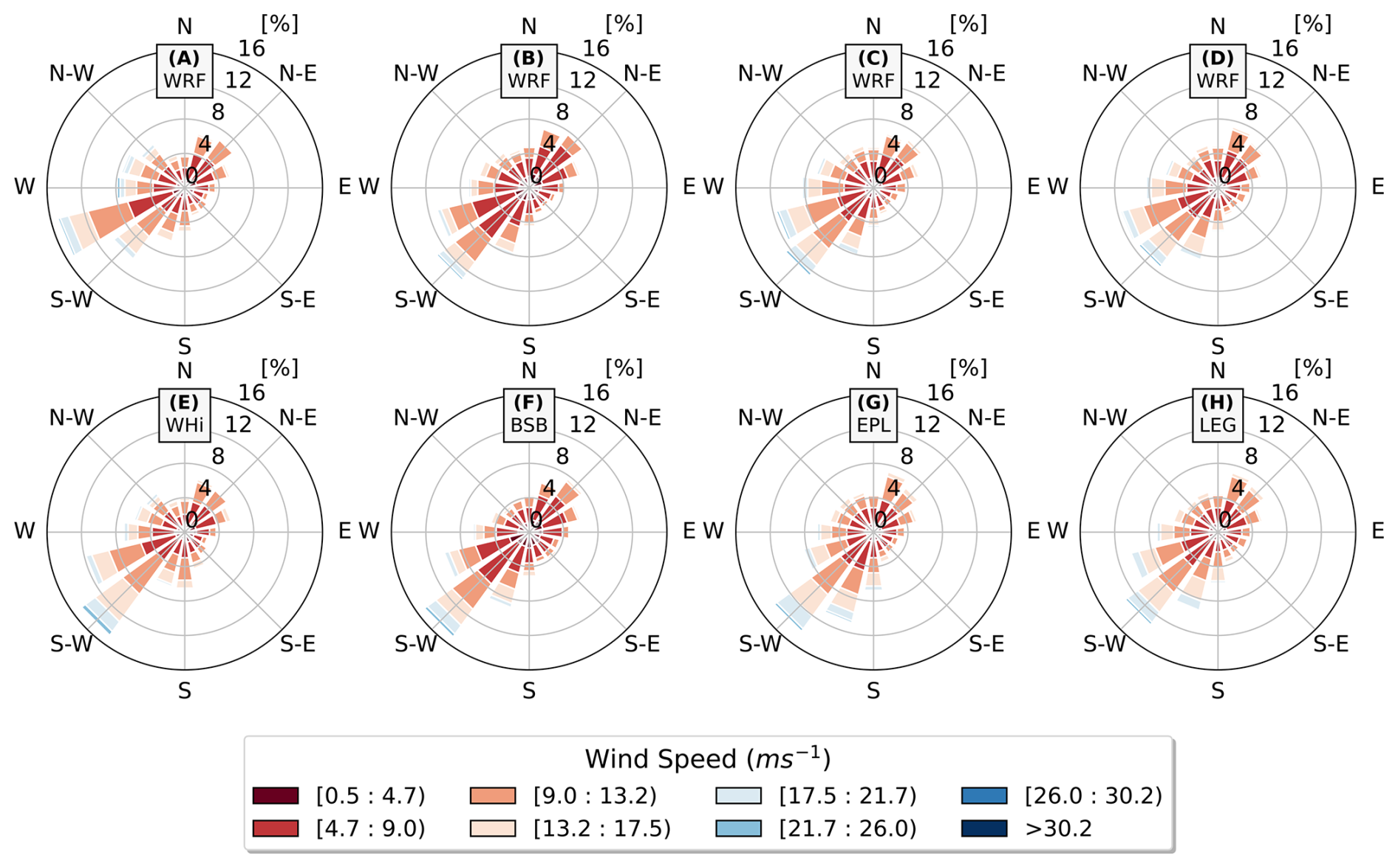
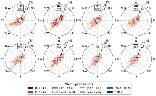
Figure 4Top: wind roses calculated at the WHi (A), BSB (B), EPL (C), and LEG (D) probe locations using the WF simulations. Bottom: wind roses extracted from the lidar measurements at WHi (E), BSB (F), EPL (G), and LEG (H). Both the lidar measurements and the model output are interpolated at the hub height.
Figure 4 illustrates the wind roses from the WF simulations (top), as well as the lidar-derived wind roses (bottom) at the analyzed locations. The investigation over the 3-year period indicates that the predominant wind direction at all locations is consistently from the southwest. At the WHi location, WRF provides a slight shift to the westerly wind direction compared to the lidar observations. A similar trend is noticed in the cases of the LEG and EPL locations, where events between the southwest to west wind directions are more prevalent in the model. Similar behavior in WRF has been reported in the work of Kalverla et al. (2019), where winds were 10° clockwise biased. At the BSB probe, the wind rose trends align between the model and the measurements, offering a highly accurate comparison with the lidar data.
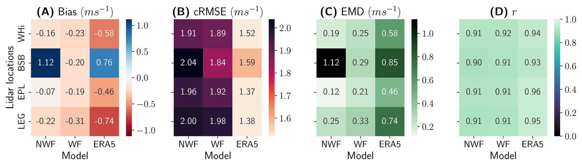
Figure 5Evaluation metrics for wind speeds against lidar data: bias (A), cRMSE (B), EMD (C), and r (D) scores. All values are interpolated to hub height. Darker colors signify poorer alignment with the observations.
3.2 Model validation with lidar observations
3.2.1 Three-year evaluation
Figure 5 presents wind speed metrics for the 3-year WRF simulations compared with lidar observations. ERA5 data, extracted from the nearest grid point and interpolated to hub height, are also shown as a baseline. Although WRF and lidar time series have a native 10 min resolution, for the aggregated analysis in this section, we upscale the datasets (WRF and lidars) to hourly averages to match the temporal resolution of ERA5. This hourly-averaged representation ensures a consistent and fair comparison of WRF and ERA5 with the lidar observations. The bias score (Fig. 5A) shows that both ERA5 and the NWF simulation exhibit a consistent negative bias at all sites except BSB, a consequence of the inherent ERA5 underestimation that propagates into WRF. The additional wind speed reduction introduced by the Fitch WFP leads to a slightly more negative bias in the WF run, although WRF generally aligns better with the lidar observations than ERA5. Part of the improved bias in the NWF runs likely results from an error-cancellation effect with the negatively biased ERA5 input, whereas in the WF simulations, these errors become slightly amplified due to wake-induced deficits but remain lower than those in ERA5. At BSB, both ERA5 and the NWF runs show a positive bias, while the WF simulation produces a smaller negative bias, corresponding to an improvement of about 82 % over NWF and 73 % over ERA5 in the near wake under the predominant southwesterly flow.
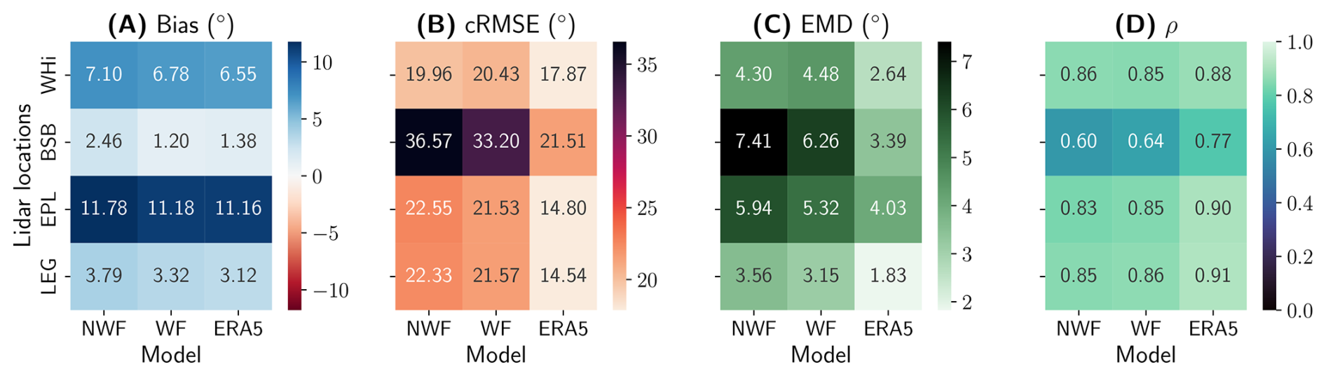
Figure 6Evaluation metrics for wind directions against lidar data: bias (A), cRMSE (B), EMD (C), and r (D) scores. All values are interpolated to hub height. Darker colors signify poorer alignment with the observations.
In contrast to the bias score, ERA5 shows a lower cRMSE than both WRF configurations, indicating that it captures the temporal variability more consistently, whereas WRF exhibits a smaller bias due to a more accurate representation of the mean flow. The EMD scores (Fig. 5C) further suggest that the WF configuration achieves the best agreement at BSB, with reductions of approximately 74 % over NWF and 65 % over ERA5. The Pearson correlation (Fig. 5D) remains high across all datasets, with minimum values of 0.90 for NWF, 0.91 for WF, and 0.93 for ERA5. Overall, both WRF and ERA5 exhibit a domain-wide negative wind speed bias, except at BSB, largely driven by the underestimation in ERA5. Consequently, wind speeds remain slightly underestimated in both the NWF and WF simulations over the full 3-year period.
Figure 6 presents bias (Fig. 6A), cRMSE (Fig. 6B), EMD (Fig. 6C), and circular correlation ρ (Fig. 6D) for wind directions, validating the WF, NWF, and ERA5 cases against the lidar observations. Both wind speed and wind direction metrics vary across the analyzed locations, with wind direction showing greater variability overall. First, it is important to highlight that the WF case yields more accurate wind direction estimates than the NWF simulations. Furthermore, when WFP is activated, wind direction bias at BSB is reduced by 51 %. At WHi, all models exhibit a consistent bias of approximately 6.5 to 7.1°, while at EPL the models show a larger bias of about 11 to 12°. The cRMSE, EMD, and ρ at BSB indicate less consistent wind direction alignment with the lidars compared to the other locations. Overall, ERA5 outperforms the WRF model in wind direction validation at the analyzed locations. The larger cRMSE in WRF compared to ERA5 is expected because the coarser ERA5 fields do not resolve kilometer-scale wind speed fluctuations, resulting in a smoother signal and lower instantaneous error. In contrast, the higher spatial and temporal variability represented in WRF leads to phase mismatches between simulated and actual wind fluctuations, producing larger instantaneous discrepancies that manifest as higher cRMSE. The study of Pronk et al. (2022) shows that ERA5 outperforms WRF simulations in terms of cRMSE and correlation coefficient, both on land and offshore, under different stability conditions. Additionally, a consistent negative bias in wind speed is reported. These findings align with the WRF sensitivity analysis of Olsen et al. (2025) in the North and Baltic seas, indicating that ERA5 outperforms the various WRF configurations in terms of cRMSE and correlation.
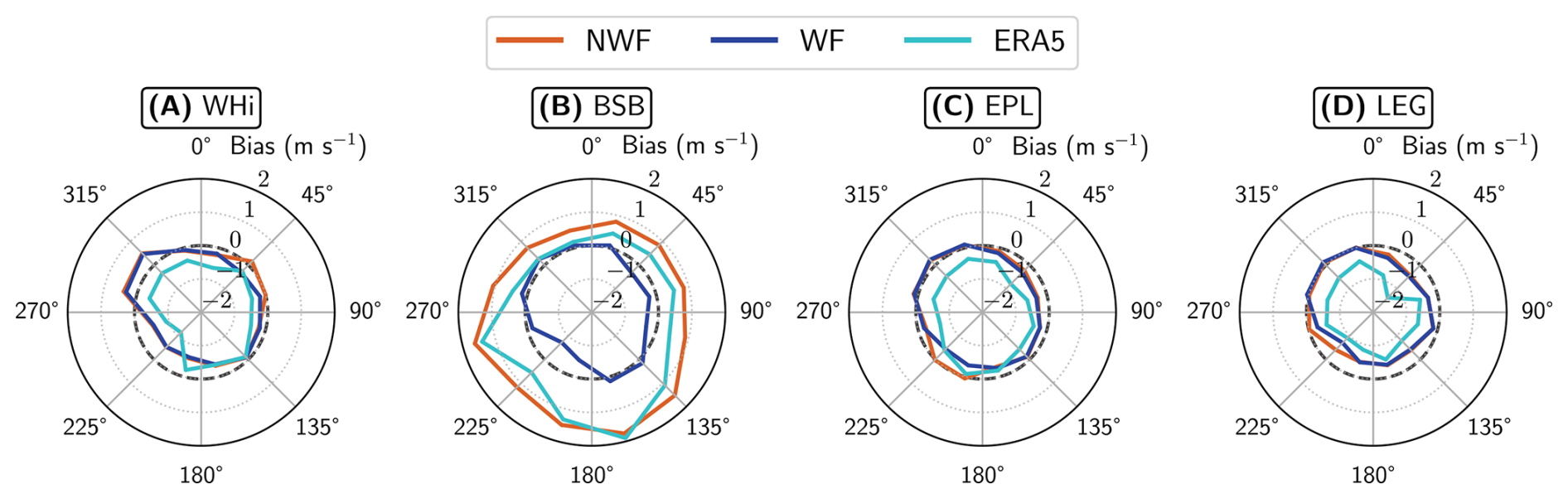
Figure 7Wind speed bias under different wind direction sectors, evaluated against lidar observations. All values are interpolated to hub height. The deviation from the dashed black line indicates the degree of misalignment with the observations.
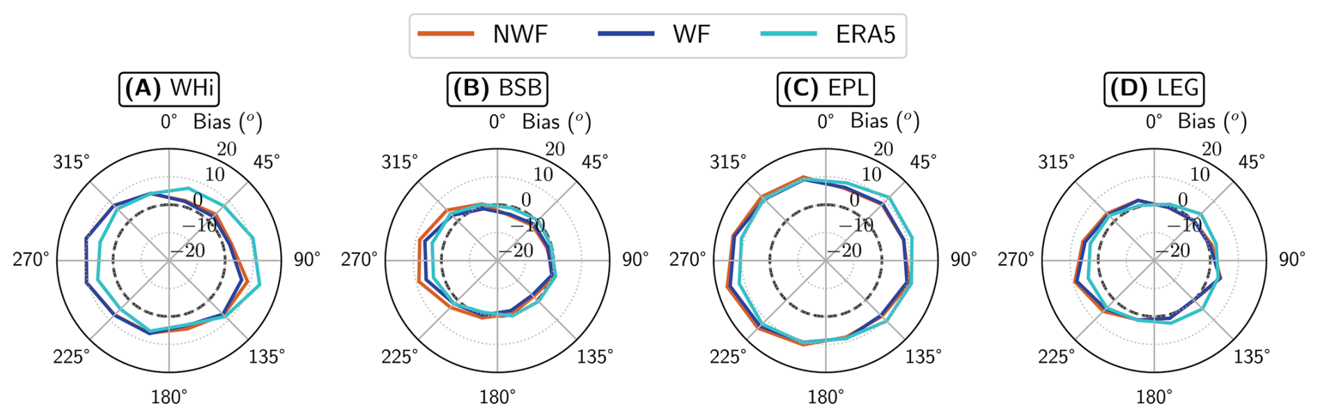
Figure 8Wind direction bias under different wind direction sectors, evaluated against lidar observations. All values are interpolated to hub height. The deviation from the dashed black line indicates the degree of misalignment with the observations.
In Fig. 7, the wind speed bias for each wind direction at each location is depicted, allowing a clearer assessment of the bias sources. Colored lines represent NWF, WF, and ERA5 datasets, and the dashed lines indicate zero bias. At WHi, EPL, and LEG, where wakes are observed due to the existence of the Belgian–Dutch cluster, the NWF and WF simulations generally show similar distributions, except along the principal wake directions, where NWF performs slightly better. More specifically, at WHi the dominant wake influence arrives from the northeast, and around 45° the NWF bias is closer to zero. A similar pattern appears at EPL and LEG, where NWF bias is closer to zero around 225 and 255°, respectively. At EPL in particular, the bias is close to zero between 190 and 225° in the NWF simulations. In all three cases, both WRF configurations reduce the negative bias found in the ERA5 data, highlighting the fact that the Fitch scheme introduces an additional bias downstream of wind farm regions. Conversely, in the intra-farm region at BSB, the Fitch scheme provides a more accurate wind speed distribution across all wind directions, underscoring its importance in strongly waked environments. This behavior of the Fitch scheme, showing prolonged wakes and enhanced wind speed deficits at locations farther downstream and more accurate wind speed distributions closer to the turbines, has also been reported in previous studies (García-Santiago et al., 2024; Ali et al., 2023).
Similar to the wind speed bias per wind direction, Fig. 8 shows the wind direction bias. Although the mean bias in Fig. 6A suggests closer agreement between the lidars and ERA5, WRF provides a better representation of the wind directions when the wind originates from the north to south-southeast (0 to 180°). Conversely, for westerly wind directions between 180 and 360°, ERA5 performs better. At BSB, the mean bias is nearly identical between the WF runs and ERA5, but ERA5 shows slightly closer agreement with the lidar measurements across all wind directions.
3.2.2 Impact of ABL stability on model performance
ABL stability conditions have been shown to play a significant role in influencing wind shear, buoyancy, and turbulence production, which in turn affect the width and length of downstream wind farm wakes (Rosencrans et al., 2024; Palatos-Plexidas et al., 2024). Therefore, it is essential to quantify these effects and assess the performance of WRF under varying ABL stratification.
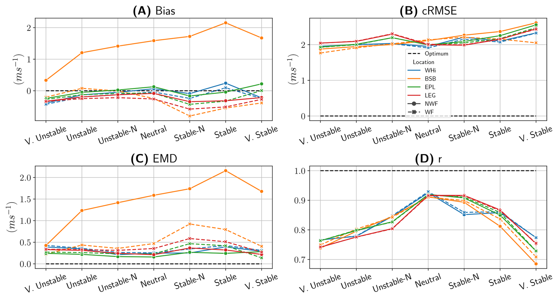
Figure 9Hub-height wind speed metrics under different stability conditions: bias (A), cRMSE (B), EMD (C), and r (D) scores. ABL classes are assessed at BSB in the NWF simulations. Solid lines denote the NWF runs, while dashed lines correspond to WF simulations. The deviation from the dashed black line indicates the degree of misalignment with the observations.
Figure 9 depicts the wind speed scores estimated at the hub height. The ABL stability classes are determined at the BSB location using the Obukhov length derived from the NWF simulations. The dashed black lines at each plot characterize the ideal score values, while the solid colored and dashed lines represent the NWF and WF simulations at each location, respectively. The EPL and LEG locations exhibit comparable patterns, with slightly greater wind speed underestimation at LEG during weakly stable to very stable conditions. In contrast, the wind speed assessed at BSB shows larger discrepancies. At this location, the influence of wind turbines in the WF simulation is more evident, where a negative bias due to the wake is always observed (wind speed is underestimated). At WHi, the WF case provides a very accurate match, especially under neutral and stable conditions where the bias is close to zero. Similar trends are also shown in the EMD scores, where reduced distribution matching appears at BSB and a closer match to observations is noticed at WHi, EPL, and LEG.
The cRMSE is around 1.8 to 2.5 m s−1 for all the cases, while there are subtle differences across the domain under different ABL conditions. Specifically, during very unstable to close-to-neutral conditions, WHi, BSB, and EPL generate a reduced cRMSE, while LEG provides the best cRMSE during stable–neutral conditions. Furthermore, the cRMSE at BSB under very stable conditions remains close to 2 m s−1 in the WRF runs. Last, correlation r is higher than 0.80 when stability conditions are near neutral and stable, while during more extreme ABL stratification, correlation values are lower and vary from 0.69 to 0.77. The increase in cRMSE under very stable conditions is also reflected in the Pearson correlation, which decreases when transitioning from stable–neutral to very stable regimes. At BSB, all wind speed metrics improve in the WF simulations relative to the NWF runs across the different stability regimes, even under very stable conditions that are known to be associated with enhanced wakes (Rosencrans et al., 2024; Ali et al., 2023; Siedersleben et al., 2020). These findings align with the correlation analysis between WRF and sonic anemometer measurements in the Horns Rev wind farm (Peña and Hahmann, 2012), which shows that model uncertainty increases as atmospheric stability deviates from neutral, i.e., under very stable or very unstable conditions. Although the Obukhov length diagnosed by the PBL scheme becomes uncertain under strongly stable conditions when Monin–Obukhov similarity theory is known to break down (Stiperski and Calaf, 2023; Optis et al., 2016) due to weak or intermittent turbulence, it remains a fundamental and practical metric for characterizing ABL stability in mesoscale models. Despite its limitations, many studies use Obukhov length, as it provides a consistent, physically based framework for classifying stability regimes and interpreting wake behavior (Rosencrans et al., 2024; Quint et al., 2025).
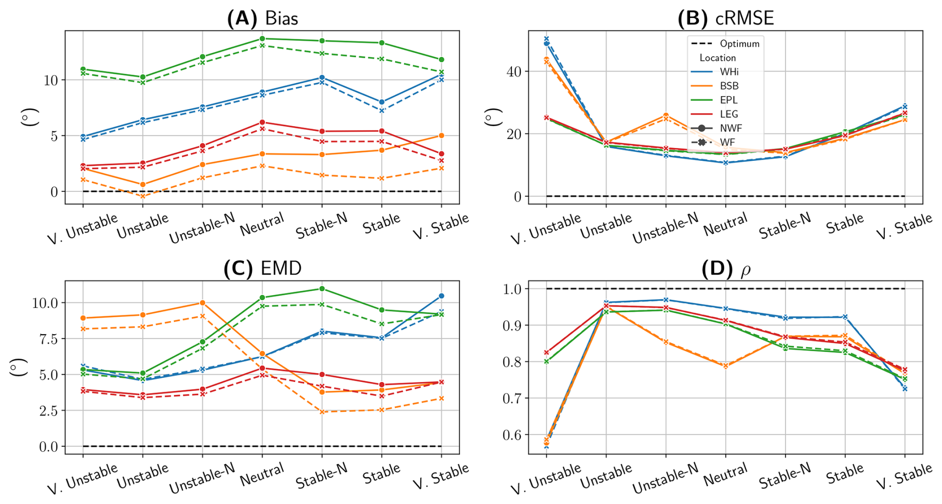
Figure 10Hub-height wind direction metrics under different stability conditions: bias (A), cRMSE (B), EMD (C), and ρ (D) scores. ABL classes are assessed at BSB in the NWF simulations. Solid lines denote the NWF runs, while dashed lines correspond to WF simulations. The deviation from the dashed black line indicates the degree of misalignment with the observations.
Wind direction scores presented in Fig. 10 indicate different trends compared to the wind speed metrics above. Focusing on the bias score, the best alignment is observed at BSB and specifically when the ABL conditions vary from very unstable to stable–neutral. The cRMSE reaches its highest values during periods of extreme ABL stratification, in both very stable and very unstable conditions, across all locations, with particularly pronounced misalignment observed at BSB and WHi during very unstable events. Furthermore, cRMSE underscores the difficulty in accurately capturing wind direction, particularly at the BSB location under unstable–neutral stratification. At BSB, EMD suggests that during very unstable to unstable–neutral conditions, there is a discrepancy of around 7.5 to 10° in the wind direction distributions, which reduces when transitioning to neutral and stable stratification. On the other hand, higher discrepancies occur during weakly stable to very stable conditions at WHi and EPL locations. Circular correlation ρ provides comparable results to cRMSE, where the model performs less accurately during very unstable and very stable conditions, and the best matching is when ABL stratification is near neutral. More precisely, during very unstable events, ρ drops down to approximately 0.58 and 10.59 at the WHi and BSB locations, respectively, indicating limited consistency in directional variability during these conditions. The high cRMSE and the low circular correlation observed at the BSB and WHi locations during very unstable events may be attributed to lower winds and enhanced turbulence. At BSB in particular, there is an important influence of the wind turbines in the flow, impacting the overall cRMSE and ρ.
The validation analysis under different stability conditions reveals differences in model performance across the various locations. We should highlight that overall the WF simulation performs better across the locations. However, in addition to the analysis aggregated over the full 3-year simulation period presented here, specific interest also lies in analyzing wind speeds across different magnitudes and specific wind directions to focus more on wake effects, as discussed in the next section.
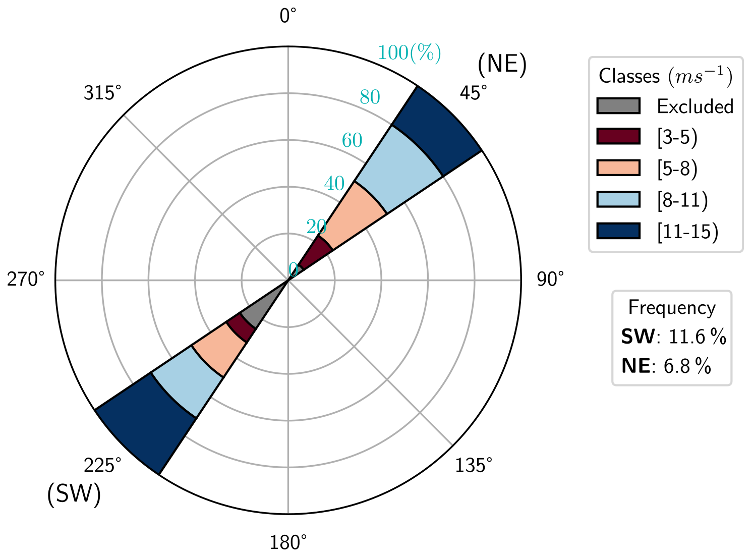
Figure 11Frequency of the wind speed classes under SW (11.6 %) and NE (6.8 %) wind directions, respectively. The frequency is calculated on the common timestamps of the lidars and not over the full period of analysis.
3.2.3 Assessment of wind speeds along the transect
In this section, we describe the influence of the wind speed magnitude on the intra-cluster and downstream wind speed deficits by comparing both the NWF and the WF simulations with lidars across the transect that connects the WHi, BSB, and EPL locations, with an almost-perfect collinear alignment of these lidars (see Fig. 2). The analysis is based on timestamps where lidar measurements are commonly available, representing about 24.4 % of the total time instances. The limitation is primarily due to the availability of WHi measurements (see Table 3). The study focuses on two predominant wind direction categories: southwest (SW) and northeast (NE), and the frequency of each wind speed class is depicted in Fig. 11. This configuration allows both SW and NE wind directions to effectively characterize the wind fields upstream and downstream of the Belgian–Dutch cluster. Both wind direction and wind speed classifications are based on the average value across the three sites (WHi, BSB, and EPL), obtained from the NWF simulations.
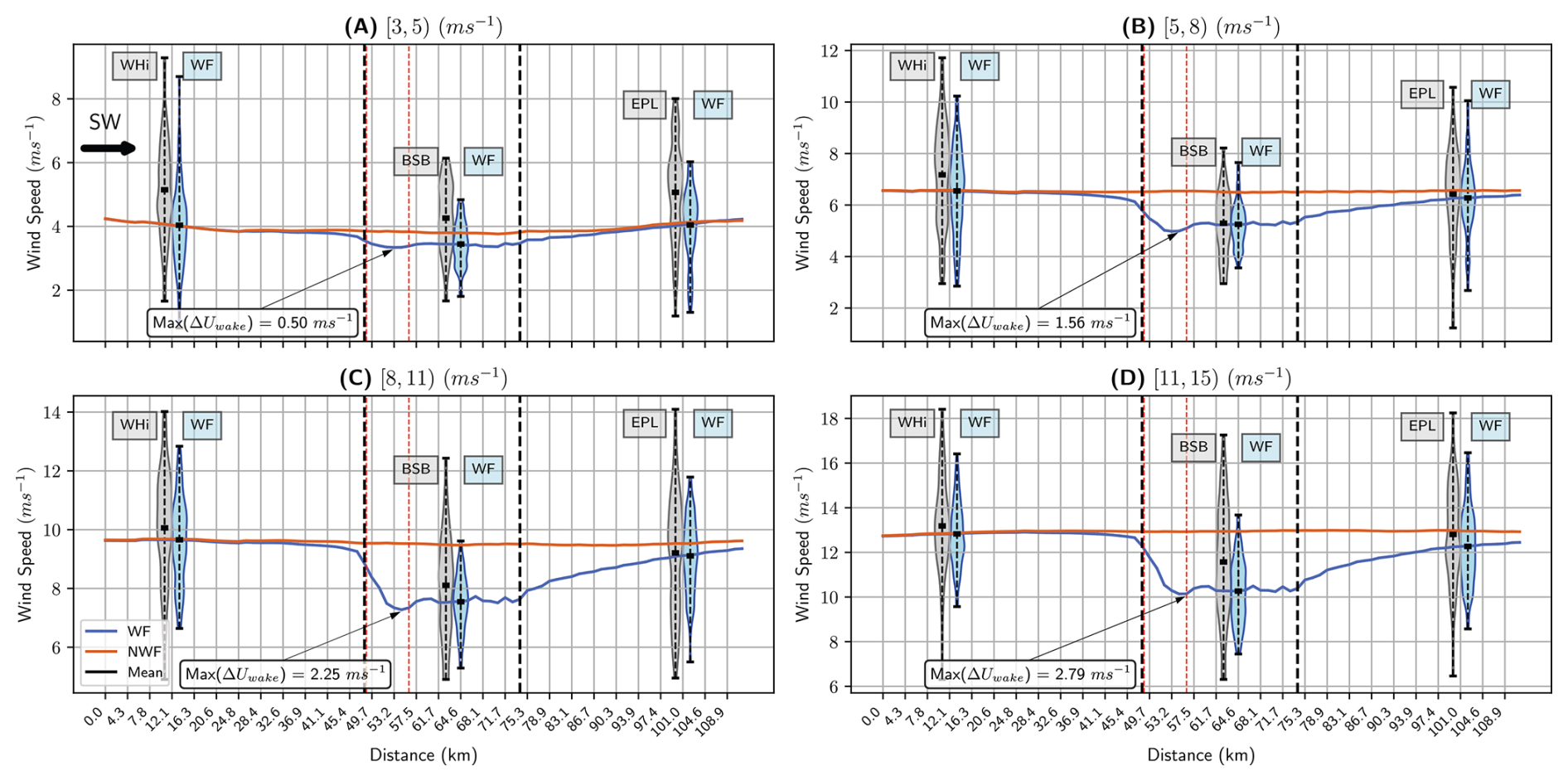
Figure 12WRF-assessed hub-height wind speed along the WHi, BSB, and EPL transect for SW wind directions, with wind direction calculated as the mean across the three lidar sites. Vertical lines mark the Belgian–Dutch cluster (black) and the Belgian-only wind farm areas (red). The wind speed range on the y axis varies across classes to highlight class-specific distributions, and the maximum wind speed deficit value within the Belgian–Dutch zone is depicted.
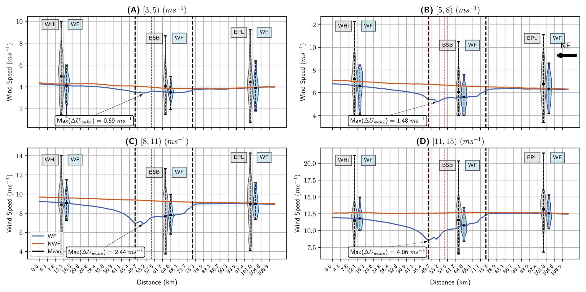
Figure 13WRF-assessed hub-height wind speed along the WHi, BSB, and EPL transects for NE wind directions, with wind direction calculated as the mean across the three lidar sites. Vertical lines mark the Belgian–Dutch cluster (black) and the Belgian-only wind farm areas (red). The wind speed range on the y axis varies across classes to highlight class-specific distributions, and the maximum wind speed deficit value within the Belgian–Dutch zone is depicted.
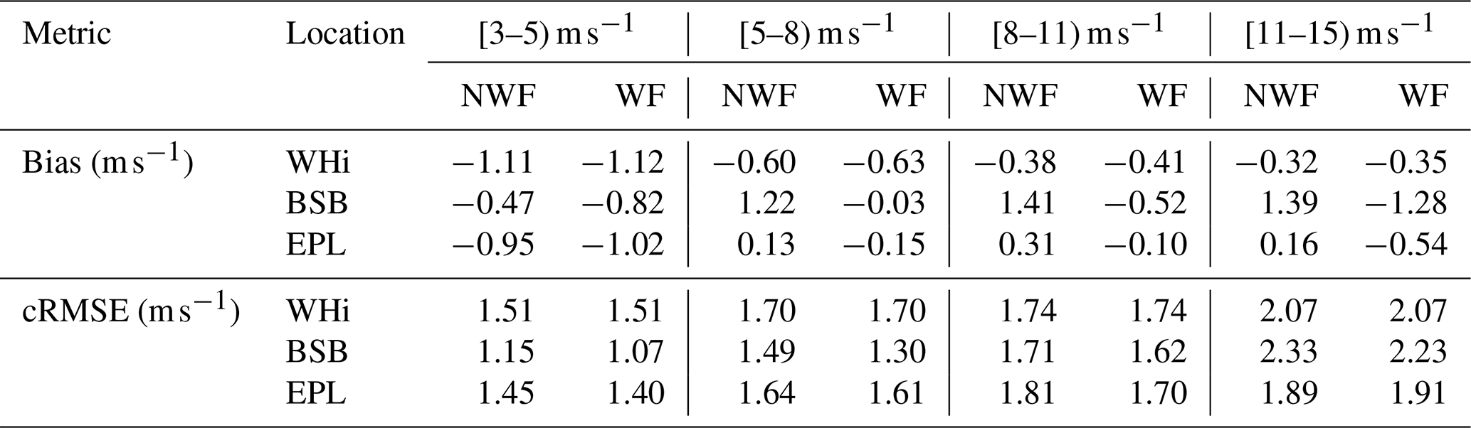
Table 4Performance metrics under the different wind speed classes for SW wind direction.
Figures 12 and 13 depict the wind speeds along the transect connecting WHi, BSB, and EPL for the four different wind speed classes under SW and NE wind directions, respectively. The distributions at each location are clipped at the 1st and 99th percentiles solely for illustrative purposes, without affecting the presented statistics. Overall, the WF simulations slightly underestimate the wind speed, and this is corroborated by the bias scores in the full-period heatmaps presented in Fig. 5A. More precisely, under SW winds, the model underestimates wind speeds at the upstream location of WHi across all the wind speed classes. Particularly when the wind speed is between [3,5) m s−1 or above 11 m s−1, the wind speed deficit, extracted by the Fitch model, is overestimated at BSB. On the other hand, the model provides a more accurate wake pattern when wind speed belongs to [5,8) and [8,11) m s−1 classes. These wind speed ranges usually correspond to the power ramp-up region of a wind turbine, where power output exhibits strong sensitivity to wind speed variations. Under northeasterly winds (see Fig. 13), the WF simulations underestimate wind speeds in both the [3,5) and the [5,8] m s−1 ranges across all locations, while performance improves markedly when wind speed varies from 8 to 11 m s−1. In both SW and NE wind direction regimes, the WF simulations overestimate the intra-farm wind speed deficit when wind speed is above 11 m s−1.
Table 4 summarizes the wind speed bias and cRMSE across the wind speed classes for the SW wind direction, highlighting how the model performance varies in upstream, intra-farm, and downstream locations. Under SW winds, where the flow progresses from WHi (upstream) → BSB → (intra-farm) → EPL (downstream), the largest errors occur upstream at WHi in the 3 to 5 m s−1 class (bias = −1.12 m s−1, and cRMSE = 1.51 m s−1, which are very similar to the WF and NWF runs), reflecting that small inflow uncertainties propagate strongly before the flow encounters the farm. As the flow moves through and downstream of the farm, the bias of the WF simulations systematically decreases at both BSB and EPL for wind speeds between 5 and 11 m s−1. The cRMSE increases with the wind speed magnitude, indicating that although the mean wind speed is well captured, the variability associated with wake turbulence and flow transitions is still not well reproduced. Overall, the cRMSE in the WF simulations is comparable to or slightly lower than that in the NWF simulations across all locations and wind speed regimes.
Table 5Performance metrics under the different wind speed classes for NE wind direction.
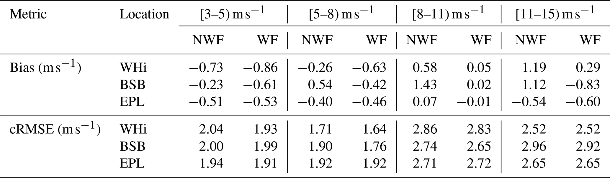
Under NE winds, where the flow reverses (EPL → BSB → WHi), a similar pattern emerges, as presented in Table 5. The upstream location (EPL) shows a reduced bias at low wind speeds (about −0.50 m s−1 in both NWF and WF) but a higher cRMSE (near 1.9 m s−1). Within the farm (BSB), bias remains modest across most wind speed classes, while cRMSE stays elevated. When wind speed is in the 8 to 11 m s−1 class, WF provides an almost negligible bias at both EPL and BSB. At higher wind speeds (above 11 m s−1), both bias and cRMSE increase, especially at BSB, although the WF simulations still yield more accurate bias at intra-farm and downstream locations. The improved bias in the NWF simulations and under specific wind speed magnitudes can be associated with error cancellation of the already-biased ERA5 data (see Sect. 3.2.1). The differences in bias and cRMSE scores between the NWF and WF simulations at the upstream locations (WHi under SW wind directions and EPL when wind comes from the northeast) are related to the fact that the flow can already be slightly affected by the UK wind farms on the west and the Dutch cluster on the NE, as presented in Fig. 1B.
Although Figs. 12 and 13 present transects under different wind speed magnitudes for the SW and NE wind directions, transect-based analyses of instantaneous wake events have also been reported using flight measurements (Ali et al., 2023; Fischereit et al., 2024). Those studies showed that the Fitch WFP in WRF can reproduce the wake features and reduce wind speed biases along transects. The transects in Figs. 13 and 14 extend this type of analysis but rely on lidar observations rather than flight data, allowing for a comparison of more events and analyzing upstream, intra-farm, and downstream wake characteristics.
Notably, distinct intra-cluster wake patterns emerge under SW and NE wind conditions. Under SW winds, the strongest wind speed deficit originates within the Belgian wind farm cluster and remains nearly unchanged as the flow proceeds across the Borssele zone. In contrast, under NE winds, the wind speed decreases progressively throughout the entire wind farm region, beginning in the Borssele cluster and intensifying as the flow enters the denser Belgian wind farms. Furthermore, the wake recovery rate is less smooth at high wind speed magnitudes. These findings highlight the directional dependence of wake dynamics and underscore the need for improved model representation of low-speed flows and intra-cluster wake effects. More specifically, the maximum wind speed deficits increase with wind speed magnitude. At wind speeds above 11 m s−1, the difference between SW and NE conditions becomes substantial: under SW winds, the maximum deficit reaches approximately 2.75 m s−1, whereas under NE winds it increases to about 4.06 m s−1. At lower wind speeds (below 8 m s−1), the largest deficits in both SW and NE regimes occur near the center of the densely built Belgian wind farm zone. At higher wind speeds, however, the location of the maximum deficit shifts. Under SW winds, the strongest deficit moves toward the northeastern boundary of the Belgian zone, near the interface with the Dutch Borssele cluster. Conversely, under NE winds, the maximum deficit appears at the downstream exit of the Belgian wind farm cluster. These contrasting behaviors between the wake trends under SW and NE wind directions arise from the strong dependence of wake evolution on turbine spacing. The averaged density of the Belgian wind farms that the analyzed transect crosses is about 10 to 12 MW km−2, while the Borssele cluster has a density of about 4 to 5 MW km−2. Therefore, the dense Belgian cluster produces rapid wake merging and a deeper cumulative deficit, whereas the more widely spaced Borssele layout allows partial recovery before wakes redevelop downstream. As a result, SW winds encounter an already-merged wake that weakens over the coarse Borssele area, while NE winds first traverse the coarse Borssele layout, where deficits remain modest and then intensify sharply upon entering the dense Belgian cluster.
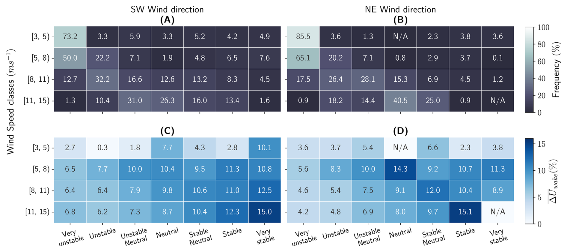
Figure 14Frequency of the ABL stability conditions for each wind speed regime, under SW (A) and NE (B) wind directions. The stability regimes based on L are computed as the average of the WHi, BSB, and EPL from the NWF simulations. Plots (C) and (D) show the averaged wake magnitude across the three locations for different ABL conditions and wind speed classes under SW and NE wind directions, respectively. Note that N/A denotes not available.
Figure 14A and B present the frequency of the ABL stability conditions under the different wind speed ranges for SW and NE wind directions, respectively. The ABL stability classification is based on Obukhov length, averaged across the three lidar probes in the NWF simulations. Under low-wind-speed conditions, very unstable and unstable events tend to dominate. Conversely, a transition toward near-neutral ABL stratification under high wind speeds is also evident. Previous studies (Rosencrans et al., 2024; Palatos-Plexidas et al., 2024; Porchetta et al., 2024) have demonstrated the dependence of wake propagation and wind speed losses on ABL stability, showing that when transitioning from neutral to stable and very stable stratification, wakes tend to extend further downstream of wind farms. Similarly, we underscore the relation between wind speed magnitude, ABL stratification, and wake propagation, where during high wind speeds, the frequency of neutral and stable events is enhanced, and wakes propagate a few tens of kilometers downstream of the Belgian–Dutch cluster.
In addition to the frequency of the stability regimes, in Fig. 14C and D, the magnitude of the average normalized wind speed deficit is presented under the different stability conditions. The wind speed deficits are estimated as the average across the three analyzed lidar locations. It is observed that under very unstable and unstable occurrences, the wake magnitude is relatively lower (varying from 2.7 % to 8.3 %). Higher wake magnitudes are observed under near-neutral ABL stratification, with wind speed deficits increasing as conditions transition from unstable to neutral and stable. However, this should be interpreted together with the frequency of events in each wind speed class, which shows that the number of very stable cases, where wake effects are relatively strong, is not particularly large. On the other hand, the wind speed deficits during very unstable and unstable events that occur more frequently (especially when wind speed is below 8 m s−1) are significantly lower. Near-neutral conditions occur more frequently when wind speed is above 8 m s−1 in both SW and NE wind direction, and the wake magnitude in these cases ranges from about 7 % to 12 %. Greater wind speed magnitudes are associated with more pronounced downstream wind speed deficits (see Figs. 12 and 13), as higher wind speeds in this region occur more frequently under neutral to stable conditions. Under these regimes, particularly during stable conditions, reduced turbulent mixing limits wake recovery, leading to enhanced and more persistent wakes (Rosencrans et al., 2024; Ali et al., 2023; Siedersleben et al., 2020). The transition toward neutral and stable ABL conditions with the increasing wind speed may contribute to the higher cRMSE values observed in Tables 4 and 5, as these regimes are associated with enhanced shear.
3.2.4 Wake characteristics and blockage effects in the Belgian–Dutch cluster
The analysis presented in the previous section, based on SW and NE wind directions, supports the investigation of the two-dimensional wake characteristics and blockage effects within the Belgian–Dutch wind farm cluster. A reduction in wind speed upstream of the wind farms is evident under both SW and NE wind directions. In the transect under SW winds (Fig. 12), a noticeable wind speed deficit begins approximately 8 km upstream of the wind farm within the 5 % wind speed deficit region. This reduction is present across the different wind speed magnitudes but becomes more rapid around 4 to 5 km upstream, particularly when wind speeds exceed 5 m s−1. For NE wind directions (Fig. 13), the blockage effect is also visible, though it is confined to a smaller region, approximately 2 to 3 km upstream of the Borssele wind farm.
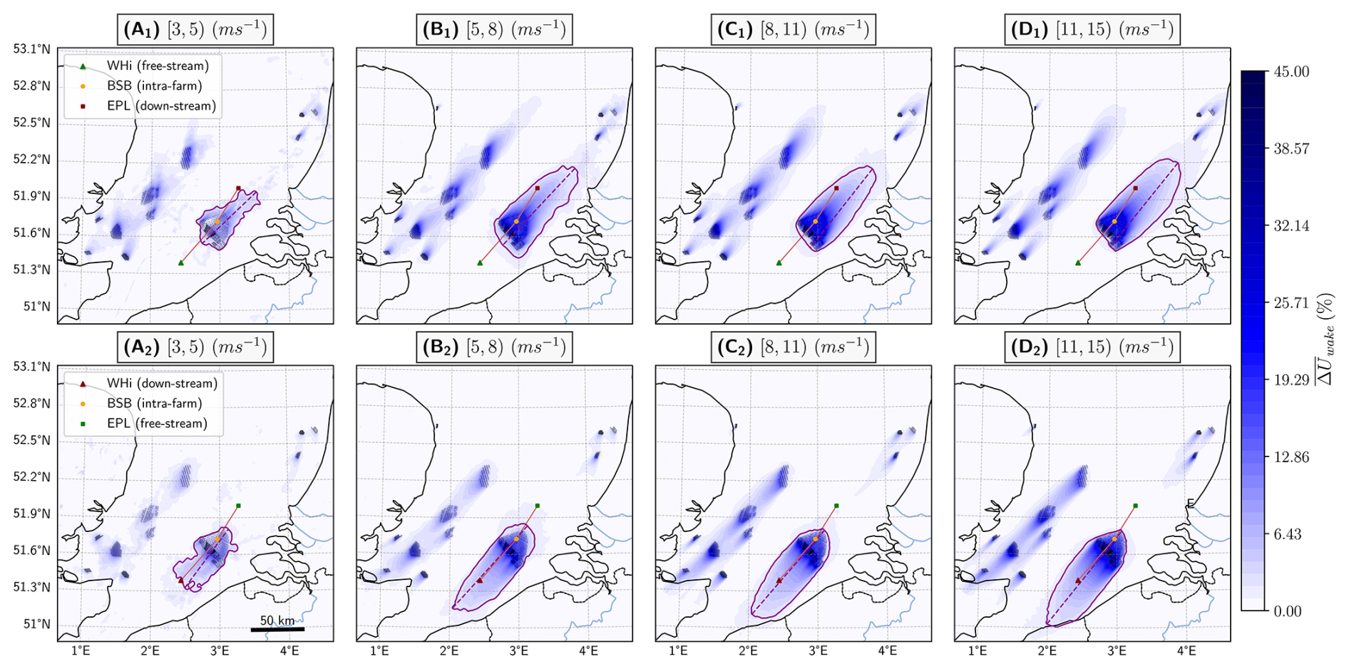
Figure 15Wind speed deficits calculated at the hub height under the four wind speed regimes. The orange line illustrates the WHi, BSB, and EPL transect. Subscript 1 indicates that wind direction is SW (top), and subscript 2 denotes NE wind direction conditions (bottom). Wind speed deficits are averaged across each wind speed class. The solid purple lines depict the 5 % wind speed deficit, and the dashed purple lines show the maximum wake length within this area.
Table 6Wake characteristics under the different wind directions and wind speed classes. The wake area corresponds to the 5 % wind speed deficit region shown in Fig. 15, while the wake length is defined as the maximum extent within this area, indicated by dashed lines.

The wake maps in Fig. 15 further confirm the presence of blockage effects under both SW and NE wind conditions. The solid purple lines indicate the 5 % wind speed deficit area, while the dashed purple lines represent the maximum wake length within this area for each wind speed regime and wind direction. The wake structures become less coherent at wind speeds below 5 m s−1, while an induction zone defined by the 5 % wind speed deficit region is observed in low wind speeds. More precisely, the maximum blockage distance from the front row of the wind turbines appears at around 10 km under the SW wind direction (Fig. 15A1), whereas it appears at around 5 km in the NE wind direction regime (Fig. 15A2). In addition, Table 6 presents the values of the 5 % wind speed deficit area and the maximum wake length within this area. The largest coherent wake region is extracted using connected-component labeling. Its perimeter is obtained from the contour of the binary mask, and the maximum extent is computed as the convex-hull diameter of the perimeter points. The estimation of both the 5 % wind speed deficit area and the maximum wake length near SW or NE wind directions is performed using the SciPy Python package (Virtanen et al., 2020). The values under the different wind speed regimes in Table 6 are comparable for both SW and NE wind directions.
When the flow transitions to higher wind speeds (above 5 m s−1), the wake structures become more coherent, leading to overall longer wake lengths (see Table 6). In the 5 to 8 m s−1 class, a blockage region forms upstream of the turbines, extending approximately 8 to 9 km from the first row under both SW and NE conditions. At higher wind speeds, this blockage pattern becomes negligible, and the flow tends to deflect around the cluster and propagate farther downstream.
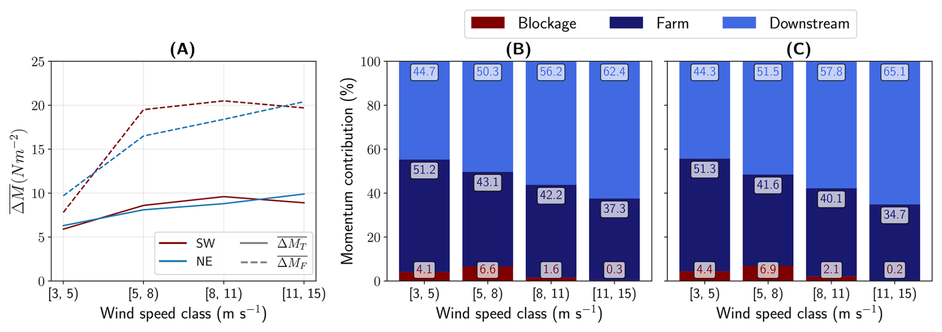
Figure 16(A) Momentum flux deficits across the total 5 % wind speed deficit region () and the Belgian–Dutch cluster area (). Momentum flux deficit fractions within the 5 % wind speed deficit area under SW (B) and NE (C) wind directions across different wind speed regimes. The farm area is the only source of momentum due to the Fitch WFP scheme. The contributions of blockage, farm (i.e., momentum extraction), and downstream momentum flux deficits are depicted using the numbers at each bar.
Figure 16 summarizes the momentum flux deficit characteristics within the 5 % wind speed deficit area. We apply Eq. (4) using hub height wind speeds extracted from the WF simulations, with evaluated over the total 5 % wind speed deficit area and over the Belgian–Dutch cluster area only to isolate the momentum extraction due to the wind turbines. Both and increase with wind speed (Fig. 16A) due to enhanced turbine-induced momentum extraction at higher wind speeds. Under the NE wind direction, where the flow interacts first with the coarser Borssele zone, the overall momentum flux deficits ( and ) display a more consistent, near-linear increasing trend over the wind speed range of 5 to 15 m s−1. The fractions of blockage, farm (i.e., the actual momentum source), and downstream momentum flux deficit distributions over the total 5 % wind speed deficit area are presented in Fig. 16B (SW) and 16C (NE). An increase in momentum flux deficit within the blockage zone is observed for wind speeds between 5 and 8 m s−1. Furthermore, although higher wind speeds enhance momentum extraction from the wind farms, the concurrent expansion of the 5 % wind speed deficit area results in a larger fraction of the momentum flux deficit being distributed downstream of the wind farms.
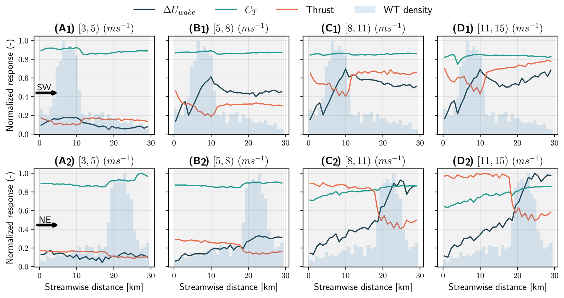
Figure 17Streamwise-averaged and normalized ΔUwake, CT, and thrust computed based on Eq. (5). The gray-shaded area extending to about 28 km represents the length of the Belgian–Dutch cluster, while the light blue bins depict the streamwise-averaged wind turbine density. The top row shows cases with SW wind direction, and the bottom row corresponds to the NE wind direction.
Figure 17 presents the streamwise normalized wind speed deficit ΔUwake, thrust, and turbine CT within the Belgian–Dutch cluster. All streamwise quantities are averaged over the spanwise direction, considering only grid points corresponding to wind turbine locations (i.e., excluding surrounding flow regions without turbines). The thrust coefficient CT is computed utilizing the CT curves provided in the wind turbine files used for the Fitch simulations (see Table A1). Consistent with the preceding analysis, all quantities are estimated using wind speeds at a uniform hub height of 107 m. The streamwise-averaged wind turbine density is shown in the light blue bins, with higher density indicating the Belgian offshore zone. Under SW wind directions and low-wind-speed regimes (Fig. 17A1), an increase in ΔUwake is observed, accompanied by a decrease in thrust as the flow crosses the dense Belgian offshore zone. The wind speed deficit then decreases within the coarser Borssele zone, consistent with the prevailing very unstable stability conditions presented in Fig. 14A. Although the trends in the streamwise wind speed deficit and thrust curves are similar at higher-wind-speed regimes, for wind speeds between 11 and 15 m s−1 (Fig. 17D1), ΔUwake shows a slight increase within the Borssele zone that can be associated with the transition to neutral and stable conditions (see Fig. 14A).
Under NE wind speeds, the streamwise trends differ, as the flow first encounters the coarser Borssele zone. Similarly to SW regimes, for wind speeds below 5 m s−1, the wind speed deficit remains relatively low, likely associated with prevailing very unstable conditions that favor faster wake recovery, even within the Borssele zone. In the 5 to 8 m s−1 wind speed regime, there is a more gradual increase in the wind speed deficit, resulting in a decrease in thrust that begins to stabilize within the Belgian offshore zone. The trends at wind speeds between 8 to 11 and 11 to 15 m s−1 are consistent, with a modest increase in thrust at higher wind speeds.
Overall, across all cases, higher wind speeds are associated with increased ΔUwake and thrust, followed by a transition to neutral and stable conditions. The thrust coefficient CT remains generally constant, showing minor increases in denser-turbine regions. For the NE wind direction at high wind speeds, CT is lower in the front rows of the Borssele wind turbines, likely due to the higher inflow velocities. Furthermore, the slight increase in ΔUwake observed in the front rows may reflect the development of the turbine induction zone. The complex layout of the Belgian–Dutch cluster results in notable differences between the SW and NE wind directions and varying wind speed conditions.
Table 7Description of the atmospheric conditions on the SAR-WRF comparison timestamps. Obukhov length L and PBLH are estimated from the NWF simulations.


Figure 18Two-dimensional wind speeds at 10 m height: SAR images (left, subscript 1), WF simulations (middle, subscript 2), and NWF simulations (right, subscript 3). Four snapshots are compared where the wind-farm-produced wake is present. The red line depicts the transect connecting the WHi, BSB, and EPL locations.
3.3 Comparison of wake events with SAR data
In this section, we focus on a one-by-one comparison of the WRF model output with SAR data. SAR images are retrieved from Sentinel 1A and 1B satellites as explained in Sect. 2.3.2, and they provide wind speed fields at 10 m height. Four specific timestamps have been selected to analyze the wind speed patterns derived from SAR and WRF data, as well as to validate the model performance across the transect that connects the WHi, BSB, and EPL lidars (see Fig. 2). These timestamps were selected manually based on the visual appearance of wind farm wakes in the SAR images. Although an average of 8 to 10 snapshots per month (see Sect. 2.3.2) covers the analyzed region, the focus on wake events affecting the WHi, BSB, and EPL lidar sites under the SW and NE wind directions resulted in a further reduction in the available snapshots. Therefore, an additional event from September 2020, outside the defined 3-year simulation period, has been deliberately included for analysis. The exact dates, times, and ABL stratification conditions derived from the NWF simulations, based on the Obukhov length and the planetary boundary layer height (PBLH), are provided in Table 7. Although this study uses only four specific SAR scenes and does not explicitly evaluate SAR data reliability, previous validation works provide strong evidence supporting the accuracy of SAR-retrieved winds. For example, Hasager et al. (2011b) compared SAR-derived wind speeds with meteorological mast measurements in the Baltic Sea and reported a small bias of −0.25 m s−1 and a correlation coefficient of R2=0.783 across 900 images. Similarly, de Montera et al. (2020) assessed 1544 SAR Level-2 Ocean product instances against four offshore buoys and three coastal weather stations around Ireland, finding an average bias of −0.4 m s−1.
Figure 18 presents the comparison of SAR and WRF wind fields at 10 m height. The left column shows the SAR-derived wind speeds, denoted by a subscript 1. The middle column depicts the WF wind speeds, indicated by a subscript 2, and in the right column, the reference NWF wind speeds are illustrated and denoted with a subscript 3. In case A, higher wind speeds are also related to stable–neutral conditions and a shallow boundary layer (see Table 7). The wake structure of the Belgian–Dutch wind farm cluster is well captured by the WF simulation. However, a slight deviation in wind direction is observed in WRF, exhibiting a positive bias toward more westerly flow. A similar bias has also been highlighted in the wind roses (Fig. 4) and in the wind direction validation heatmap in Fig. 6A. The prolonged wake extending more than 50 km downstream under stable–neutral stratification agrees with the findings of Cañadillas et al. (2020) and Platis et al. (2018), who also report that wake structures are more pronounced and longer during stable conditions. Furthermore, Siedersleben et al. (2020) examined a stable event simulated with the Fitch scheme in WRF (version 3.8.1), comparing the original formulation (a=1) with a variant excluding the added TKE term, and showed that including the added TKE source under stable stratification results in a more realistic representation of the prolonged wake of a SAR-retrieved 10 m wind speed pattern. In our study, although we use a finer grid spacing (1 km instead of 1.67 km) and a reduced TKE coefficient (a=0.25), which limits the influence of the added TKE term, we observe very good agreement between the SAR image and the WF simulations during stable conditions. Furthermore, Ali et al. (2023) evaluated several WFP schemes to characterize the wake of a specific event using 10 m wind speeds from SAR data. Their results show that, when comparing the Fitch model with a=1 and a=0.25, the latter produces a longer wake downstream of the wind farms, similar to the behavior observed in case A analyzed in the present study.
In case B, the wake is weaker but still detectable both in the SAR image and in the WF simulation. In this case, stability conditions are very unstable, and the PBLH is around 700 m, explaining the attenuated wake pattern. Case C is characterized by higher wind speeds, L varies from −300 to −450 m, and PBLH is approximately 300 m across the three locations, resulting in a more unstable–neutral stratification profile, resulting in the observed downstream wake of about 40 to 50 km. Similar but shorter wake patterns of about 25 to 35 km have been observed during neutral stratification in the study of Platis et al. (2018). Last, in case D, very unstable ABL conditions prevail, and the PBLH varies between 250 m upstream at the WHi location and 358 m downstream at the EPL area. This is the only SAR image with clear wakes for SW wind conditions. Overall, the patterns of the wakes are accurately represented by the WF simulations, highlighting the importance of using the Fitch WFP scheme in WRF. Although SAR assumes neutral stability to compute the 10 m wind speed, there are discrepancies with the WRF model, especially in cases B and D, where very unstable stratification dominates based on the values of Obukhov length. Uncertainty exists regarding the assumption of SAR image neutrality used to calculate wind fields, an issue that has also been reported in previous studies across different applications (Hasager et al., 2011a; Ahsbahs et al., 2017). Furthermore, there is uncertainty in the estimation of L within WRF, as it strongly depends on the PBL and surface schemes applied in each configuration.

Figure 19Wind speeds along the WHi, BSB, and EPL transects. Comparison between WF (purple), NWF (orange), and SAR (green) at 10 m height, including lidar observations at 107 m height (scatter points) along the transects where available. Similar to Figs. 12 and 13, the vertical black and red dashed lines indicate the Belgian–Dutch cluster and the Belgian zone only, respectively.
Table 8Mean absolute error (MAE) and point-wise lidar absolute error (AE) for the NWF and WF simulations. MAE is computed across the upstream, intra-farm, and downstream regions of the transects shown in Fig. 19. The intra-farm region corresponds to the full Belgian–Dutch cluster, delineated by the two vertical dashed black lines.

a WHi is downstream and EPL upstream; b WHi is upstream and EPL downstream. N/A: not available.
In addition to the wind speed deficit maps, Fig. 19 presents the transects that connect WHi, BSB, and EPL. The green line illustrates the 10 m height SAR wind speeds, while the purple and orange lines correspond to the WF and NWF simulation outputs, respectively. Although a Hampel filter (see Sect. 2.3.3) is applied to the transect of the SAR data, we can still observe a few outlier values, especially in the intra-farm area. The wind turbines generate spikes in the wind fields due to strong radar reflection (Hasager et al., 2015; Ahsbahs et al., 2020). Therefore, to further evaluate the performance of the WRF model, hub-height lidar measurements are incorporated when available, depicted as gray scatter points in Fig. 19. In addition to the qualitative assessment of the wind speeds in Fig. 19, Table 8 presents the MAE across the upstream, intra-farm, and downstream transect regions, as well as the point-wise AE, when lidar measurements are available, and the evaluation methodology is described in Sect. 2.3.4. In cases A, B, and C (NE wind flow), the transect follows the direction EPL (upstream) → BSB (intra-farm) → WHi (downstream), whereas case D corresponds to a SW flow event, where the sequence reverses.
Case A shows good agreement in the representation of the transect wake. Specifically, while the WF simulation tends to underestimate wind speeds upstream and within the Borssele zone, it accurately captures the wind speed deficit in the Belgian wind farms and downstream of the wind farm cluster. This is also reflected in Table 8, where WF generates a slightly higher MAE only in the upstream region, with MAE = 0.49 m s−1 compared to MAE = 0.37 m s−1 in the NWF simulation. However, the improvement between the WF against the NWF simulations in MAE in the intra-farm region and downstream is 81 % and 85 %, respectively. Similarly, in Case B, both the intra-farm and the downstream wind speed patterns are well represented by the WF simulation. Although the overall trend is accurately reproduced, the WF simulation tends to overestimate the wind speeds upstream and downstream of the wind farms. Additionally, a flow acceleration is observed as the wind exits the Belgian–Dutch cluster. This pattern is consistent with the broader flow conditions downstream of the Belgian–Dutch cluster, since a similar acceleration is evident in the SAR observations and in both the WF and the NWF simulations. Both the lidar measurements and the WF simulation effectively capture the intra-farm wind speed deficit and the downstream flow acceleration. Furthermore, in Table 8, MAE and AE are better in the WF simulation than in the NWF simulation across the full transect regions.
Case C also features NE-incoming wind conditions. Similar to the previous cases, the WF simulation successfully captures the wind speed deficit trends both within the intra-cluster zone and in the downstream wake recovery region. Both the NWF and the WF simulations show noticeable discrepancies upstream at EPL compared to lidar observations, with an AE reaching above 3 m s−1. This is significantly improved both at BSB and downstream at WHi, where WF simulations outperform the NWF runs in terms of both MAE across the transect regions and AE against the lidar measurements. During this event, the Obukhov length at EPL is relatively high and negative, indicating unstable to near-neutral conditions. This may be attributed to less negligible shear, which can contribute to increased deviations from the lidar measurements. In the NWF simulation, an unrealistic and nearly linearly increasing pattern in wind speed of approximately 0.5 m s−1 between EPL and WHi is observed. Case D is the only selected timestamp with a SW wind direction. Although the SAR data exhibit considerable noise, particularly within the intra-farm region, the WF simulation is still able to reproduce the wind speed deficit and the downstream wake recovery trend. In this case, only EPL lidar measurements are available, which show good agreement with the WF simulation, with a slightly improved AE compared to the NWF run. Furthermore, the MAE provides a more accurate matching with the 10 m SAR wind speeds across the three transect regions in the WF simulations.
This study incorporates high-resolution mesoscale simulations using WRF coupled with the Fitch WFP scheme over a 3-year-long period (2021–2023), focusing on the Southern Bight of the North Sea. The performance of the model is evaluated across the full 3-year simulation period, with additional analysis presented under varying ABL stability conditions and wind speed magnitudes. Furthermore, the model-simulated wind speeds are compared against 10 m wind speeds derived from SAR data for specific events. A key contribution lies in the detailed investigation of upstream, intra-farm, and downstream wake structures, utilizing both WRF model outputs and observational data at selected locations.
Our findings demonstrate that the use of the Fitch WFP scheme, in combination with this particular WRF configuration, captures the wake effects and provides an improvement in model performance relative to a simulation without wind farms at the intra-farm region. First, focusing on the time-averaged wind speeds over the full analysis period, the WF simulations yield a substantial improvement in both bias and EMD, with reductions of approximately 82 % and 73 % compared with the NWF simulations, respectively, in the intra-cluster (BSB location). Furthermore, when analyzing the wind speed bias under different wind directions, both NWF and WF configurations reduce the negative bias inherited from the ERA5 data, with the results indicating that the Fitch scheme introduces an additional deficit downstream of the Belgian–Dutch cluster. However, within the intra-farm area, the Fitch scheme provides a more accurate wind speed distribution across all wind directions, underscoring its importance for representing strongly waked environments. Beyond the improvements in bias and EMD, the WF simulations perform similarly to the NWF runs in terms of cRMSE and correlation, with only small and marginal differences. Similarly, wind direction metrics are also improved in the WF simulations, as bias is reduced by approximately 51 % at BSB, while an analysis of wind direction biases by sector reveals that WF can perform better than ERA5 for wind directions from the northeast to the south.
The ABL classification based on the values of Obukhov length indicates that very unstable conditions prevail close to the Belgian–Dutch cluster. In addition, this work highlights that when the stability conditions are near neutral, WF simulations provide an adequate comparison against the lidars, while during extreme stratification, the uncertainty in the model increases. Classifying wake events based on wind speed magnitude reveals that increasing wind speeds are associated with a transition in ABL stability from very unstable toward neutral and stable regimes, accompanied by intensified wake intensity.
Extending the analysis to wake characteristics under different wind speed regimes and focusing on SW and NE wind directions reveals several consistent patterns. First, under SW wind direction, the WF simulations accurately capture the wake structure when wind speeds range between 5 and 8 m s−1, providing an almost negligible bias at BSB and downstream at EPL. Under the NE wind direction, the optimum performance of WF simulations occurs at wind speeds between 8 and 11 m s−1. Although the model tends to overestimate intra-farm wind speed deficits at BSB under higher-wind-speed conditions, it shows comparable improvements in long-distance downstream wakes at EPL (for SW winds) and WHi (for NE winds), where smaller bias and cRMSE values are obtained. The differences in wake structure and its evaluation under SW and NE wind conditions likely reflect the influence of the densely built Belgian wind farm cluster compared with the coarser turbine spacing in the Borssele zone. Furthermore, with increasing wind speed, an overall enhancement in the 5 % wind speed deficit area and maximum wake length is observed. Momentum extraction, expressed as a momentum flux deficit within the Belgian–Dutch cluster, increases with wind speed due to the higher incoming momentum. At higher-wind-speed regimes, thrust increases, with localized reductions occurring in dense-wind-turbine regions, reflecting the corresponding decrease in wind speed. In addition, at lower-wind-speed regimes, an upstream wind speed reduction zone is observed, consistent with enhanced upstream distribution of the momentum flux deficit. As the wind speed magnitude increases, the blockage effect weakens, and the flow remains more aligned with the turbine cluster, resulting in a more coherent downstream structure.
Furthermore, a comparison with SAR images at specific events shows that WF performs well in representing the wake structure generated by the Belgian–Dutch cluster. In both the intra-farm and the wake recovery regions, WF provides a realistic wind speed deficit. To assess the performance of the model during these events, MAE and AE are computed. More specifically, MAE is estimated across the upstream, intra-farm, and downstream regions, while AE is calculated at each lidar location when measurements are available. Building on the previously discussed improvements in the qualitative wake-pattern representation, the error metrics further confirm that the WF simulations provide better alignment with observations than the NWF runs across all locations, with the most pronounced improvements occurring in the intra-farm and downstream regions.
This study can accurately evaluate the model performance by utilizing upstream, intra-farm, and downstream lidar measurements as well as SAR images at specific events. Systematic biases in both wind speed and direction are evident, particularly in the wind speed metrics. However, it should be highlighted that the model is driven by ERA5 hourly data, which consistently introduce biases, affecting the boundary conditions in WRF and propagating wind speed underestimations to the analyzed locations. In addition, due to uncertainties introduced by the PBL schemes in WRF, exploring alternative physics configurations in the future may be warranted to enhance simulation accuracy. The scope of this study is limited to using the Fitch WFP scheme combined with the MYNN 2.5 PBL scheme. Additional multi-year simulations using different WFP schemes, like the explicit wind farm (EWP) parameterization scheme (Volker et al., 2015; García-Santiago et al., 2024) applied with different PBL schemes or the induction correction to the original Fitch scheme (Vollmer et al., 2024), could also provide insights into the year-long effects of large wind farm clusters.
This work may serve as a resource for future studies, offering a comprehensive 3-year analysis of ABL stratification, wake dynamics, and model validation. The importance of mesoscale models is underscored since they can adequately describe the wake effects at large scales, where high-fidelity simulations are still impractical. In addition, the availability of measurements is essential for ensuring the reliability of numerical simulations and for quantifying associated uncertainties. Finally, further improving our understanding of wind farm wake dynamics will require both advances in wind farm modeling and more extensive measurement campaigns.
A1 Evaluation metrics
The following equations are used to calculate the wind speed metrics:
The equations used to calculate the wind direction scores are defined in this section:
The Earth Mover's Distance is assessed using the Wasserstein first distance (WD). WD is defined as a distance between two probability measures P and Q on a metric space (ℛ×ℛ) by
where Γ(P,Q) denotes the set of all couplings with marginals P and Q.
A2 WRF–Fitch sensitivity analysis
A sensitivity analysis of the turbulent kinetic energy (TKE) coefficient α in the Fitch WFP scheme is performed. Four different WRF simulations are considered: a no-wind-farm case (NWF), F0 (α=0), F0.25 (α=0.25, which represents the reference wind farm simulation used in this study), and F1 (α=1). These simulations are validated against observations from four lidar locations over the period from 15 January 2022 to 15 July 2022, in comparison with ERA5 reanalysis data.
Figures A1 and A2 present the wind speed and wind direction validation metrics, respectively. The results indicate that the F1 configuration generally provides improved performance at the BSB location. However, no single configuration consistently outperforms the others across all sites and metrics. Consequently, the F0.25 configuration is selected as the reference wind farm setup for this study, as it provides a balanced overall performance.
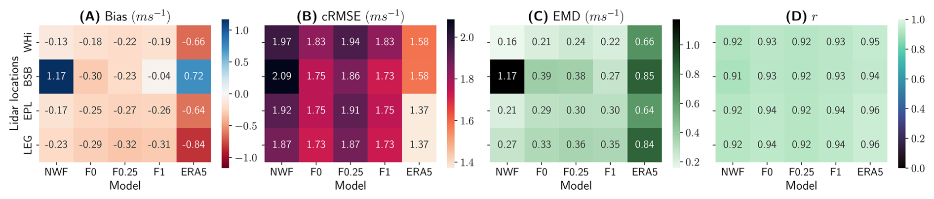
Figure A1Evaluation of hub-height wind speeds from four WRF simulations and ERA5 using observations from four lidars: bias (A), cRMSE (B), EMD (C), and r (D) scores.
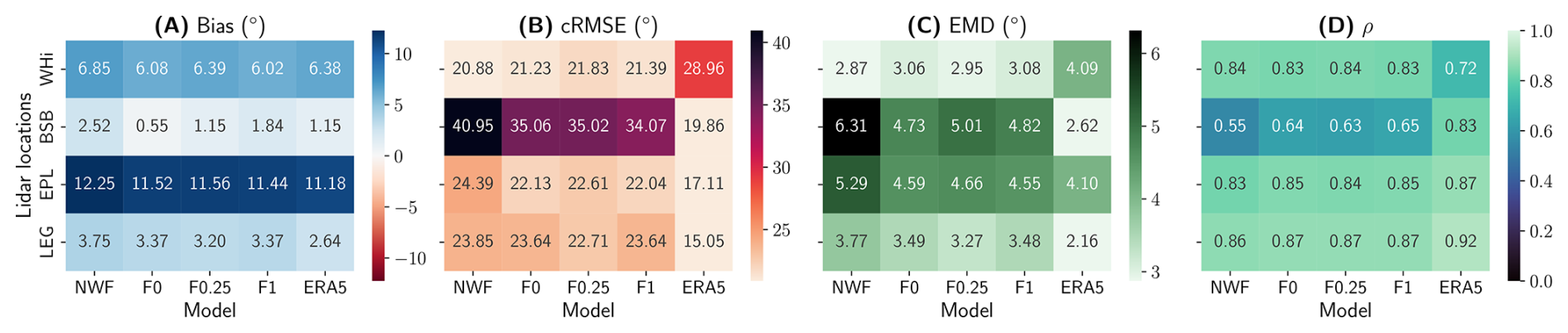
Figure A2Evaluation of hub-height wind directions from four WRF simulations and ERA5 using observations from four lidars: bias (A), cRMSE (B), EMD (C), and ρ (D) scores.
Table A1Details on the wind farms used in the model setup. Power and thrust curves remain confidential for most of the wind turbines used in the Fitch WFP.
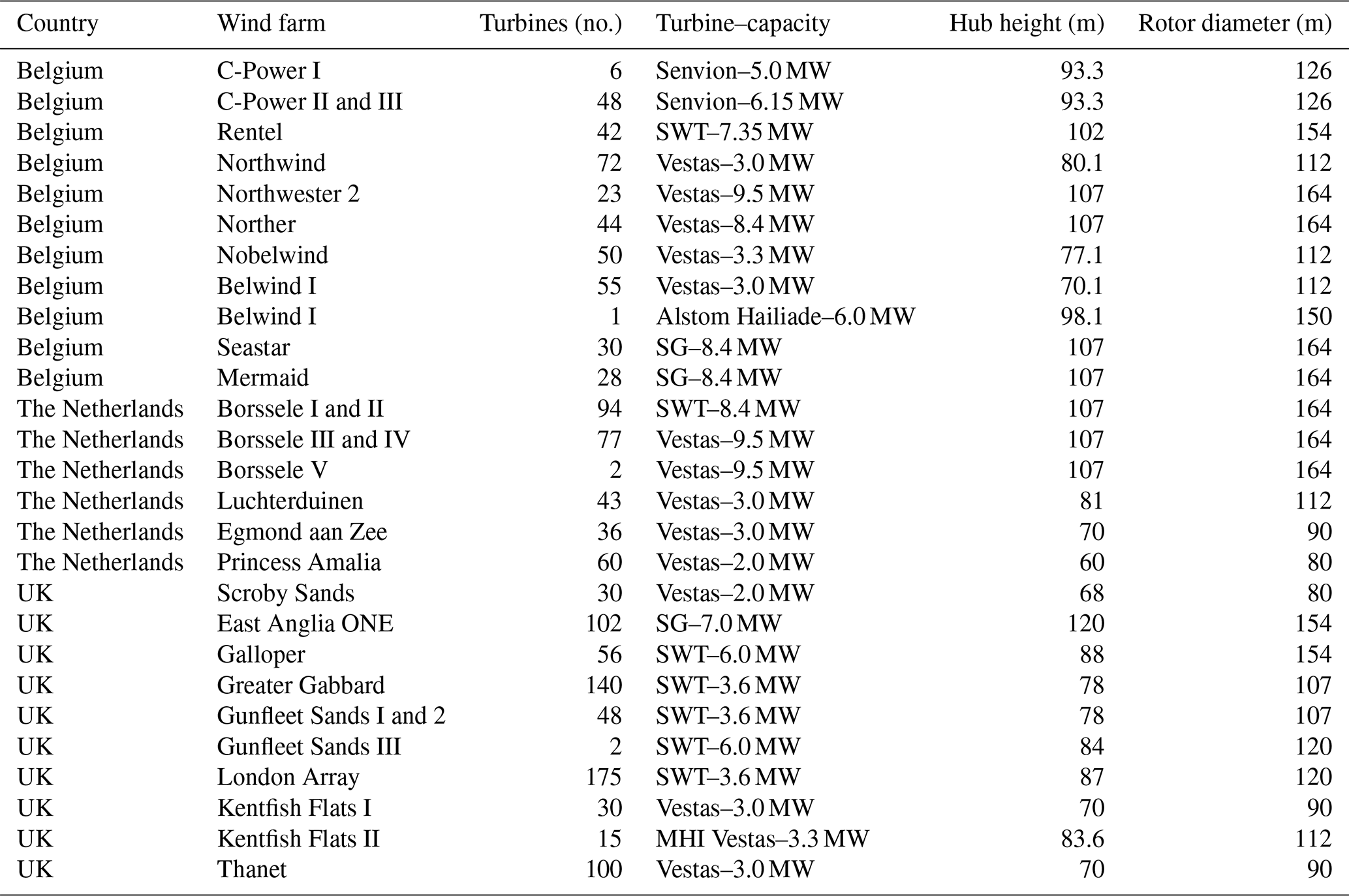
The ERA5 hourly reanalysis data (Hersbach et al., 2020) that have been used in this study are publicly available, and they can be downloaded from the Copernicus Climate Data Store at https://doi.org/10.24381/cds.bd0915c6 (Hersbach et al., 2023). WRF is an open-source model, and the version used in this study can be found on GitHub: https://github.com/wrf-model/WRF/releases/tag/v4.5.2 (last access: 4 August 2026). The files used to configure the WRF simulations can be shared upon request. The lidar profiles provided by TNO (EPL and LEG platforms) are publicly accessible: https://offshorewind-measurements.tno.nl/en/data/ (last access: 2 May 2025). The lidar profiles at the BSB platform are provided by KNMI: https://dataplatform.knmi.nl/dataset/windlidar-nz-wp-platform-10min-1 (last access: 5 May 2025). WHi (MP7) lidar profiles remain confidential.
AP-P contributed to the conceptualization, investigation, methodology, software, data curation, and writing (original draft, review, and editing of the revised versions). SG contributed to the methodology and writing (review and editing). JvB contributed to funding acquisition, supervision, and writing (review and editing). LDC contributed to methodology, supervision, and writing (review and editing). WM contributed to conceptualization, investigation, methodology, writing (review and editing), supervision, project administration, and funding acquisition.
The contact author has declared that none of the authors has any competing interests.
Publisher's note: Copernicus Publications remains neutral with regard to jurisdictional claims made in the text, published maps, institutional affiliations, or any other geographical representation in this paper. The authors bear the ultimate responsibility for providing appropriate place names. Views expressed in the text are those of the authors and do not necessarily reflect the views of the publisher.
This research has received financial support from the Flemish Government through the Agency for Innovation and Entrepreneurship (Vlaams Agentschap Innoveren en Ondernemen, VLAIO), within the framework of the Cloud4Wake project. Furthermore, this work received funding from the Federal Public Service Economy of the Belgian Federal Government through the Energy Transition Fund, under the BeFORECAST project. Lesley De Cruz acknowledges support from the Belgian Science Policy Office (BELSPO) through the FED-tWIN programme (Prf-2020-017). HPC resources are granted by the Flemish Supercomputer Center (VSC), supported by funding from the Research Foundation – Flanders (FWO) and the Flemish Government. The authors would like to acknowledge Gertjan Glabeke for the installation and processing of the Westhinder platform lidar dataset. Alexandros Palatos-Plexidas would like to acknowledge Steven Knoop for pointing out the 180° ambiguity issue for the BSB lidar.
This research has been supported by the Agentschap Innoveren en Ondernemen (grant no. HBC.2022.0549) and the Belgische Federale Overheidsdiensten (grant no. 2022-000795).
This paper was edited by Cristina Archer and reviewed by three anonymous referees.
Ahsbahs, T., Badger, M., Karagali, I., and Larsén, X. G.: Validation of Sentinel-1A SAR Coastal Wind Speeds Against Scanning LiDAR, Remote Sens., 9, https://doi.org/10.3390/rs9060552, 2017. a, b
Ahsbahs, T., Badger, M., Volker, P., Hansen, K. S., and Hasager, C. B.: Applications of satellite winds for the offshore wind farm site Anholt, Wind Energ. Sci., 3, 573–588, https://doi.org/10.5194/wes-3-573-2018, 2018. a
Ahsbahs, T., Nygaard, N. G., Newcombe, A., and Badger, M.: Wind Farm Wakes from SAR and Doppler Radar, Remote Sens., 12, https://doi.org/10.3390/rs12030462, 2020. a
Ali, K., Schultz, D. M., Revell, A., Stallard, T., and Ouro, P.: Assessment of five wind-farm parameterizations in the weather research and forecasting model: a case study of wind farms in the North Sea, Mon. Weather Rev., 151, 2333–2359, https://doi.org/10.1175/MWR-D-23-0006.1, 2023. a, b, c, d, e, f, g
Archer, C. L., Colle, B. A., Veron, D. L., Veron, F., and Sienkiewicz, M. J.: On the predominance of unstable atmospheric conditions in the marine boundary layer offshore of the US northeastern coast, J. Geophys. Res.-Atmos., 121, 8869–8885, https://doi.org/10.1002/2016JD024896, 2016. a
Archer, C. L., Wu, S., Ma, Y., and Jiménez, P. A.: Two corrections for turbulent kinetic energy generated by wind farms in the WRF model, Mon. Weather Rev., 148, 4823–4835, https://doi.org/10.1175/MWR-D-20-0097.1, 2020. a, b, c
Bergman, G., Verhoef, J., and van der Werff, P.: Lichteiland Goeree LiDAR measurement campaign, Instrumentation Report 2022, TNO, https://resolver.tno.nl/uuid:53bf464e-4538-492d-acf5-631de37adea4 (last access: 2 May 2025), 2022. a
Cañadillas, B., Foreman, R., Barth, V., Siedersleben, S., Lampert, A., Platis, A., Djath, B., Schulz-Stellenfleth, J., Bange, J., Emeis, S., and Neumann, T.: Offshore wind farm wake recovery: Airborne measurements and its representation in engineering models, Wind Energy, 23, 1249–1265, https://doi.org/10.1002/we.2484, 2020. a, b
de Montera, L., Remmers, T., O'Connell, R., and Desmond, C.: Validation of Sentinel-1 offshore winds and average wind power estimation around Ireland, Wind Energ. Sci., 5, 1023–1036, https://doi.org/10.5194/wes-5-1023-2020, 2020. a
Dörenkämper, M., Olsen, B. T., Witha, B., Hahmann, A. N., Davis, N. N., Barcons, J., Ezber, Y., García-Bustamante, E., González-Rouco, J. F., Navarro, J., Sastre-Marugán, M., Sīle, T., Trei, W., Žagar, M., Badger, J., Gottschall, J., Sanz Rodrigo, J., and Mann, J.: The Making of the New European Wind Atlas – Part 2: Production and evaluation, Geosci. Model Dev., 13, 5079–5102, https://doi.org/10.5194/gmd-13-5079-2020, 2020. a
Fischereit, J., Brown, R., Larsén, X. G., Badger, J., and Hawkes, G.: Review of mesoscale wind-farm parametrizations and their applications, Bound.-Lay. Meteorol., 182, 175–224, https://doi.org/10.1007/s10546-021-00652-y, 2022a. a, b
Fischereit, J., Schaldemose Hansen, K., Larsén, X. G., van der Laan, M. P., Réthoré, P.-E., and Murcia Leon, J. P.: Comparing and validating intra-farm and farm-to-farm wakes across different mesoscale and high-resolution wake models, Wind Energ. Sci., 7, 1069–1091, https://doi.org/10.5194/wes-7-1069-2022, 2022b. a
Fischereit, J., Vedel, H., Larsén, X. G., Theeuwes, N. E., Giebel, G., and Kaas, E.: Modelling wind farm effects in HARMONIE–AROME (cycle 43.2.2) – Part 1: Implementation and evaluation, Geosci. Model Dev., 17, 2855–2875, https://doi.org/10.5194/gmd-17-2855-2024, 2024. a, b
Fitch, A. C., Olson, J. B., Lundquist, J. K., Dudhia, J., Gupta, A. K., Michalakes, J., and Barstad, I.: Local and mesoscale impacts of wind farms as parameterized in a mesoscale NWP model, Mon. Weather Rev., 140, 3017–3038, https://doi.org/10.1175/MWR-D-11-00352.1, 2012. a, b
Flamary, R., Courty, N., Gramfort, A., Alaya, M. Z., Boisbunon, A., Chambon, S., Chapel, L., Corenflos, A., Fatras, K., Fournier, N., Gautheron, L., Gayraud, N. T. H., Janati, H., Rakotomamonjy, A., Redko, I., Rolet, A., Schutz, A., Seguy, V., Sutherland, D. J., Tavenard, R., Tong, A., and Vayer, T.: POT: Python Optimal Transport, J. Mach. Learn. Res., 22, 1–8, http://jmlr.org/papers/v22/20-451.html (last access: 22 July 2025), 2021. a
García-Santiago, O., Badger, J., and Hahmann, A. N.: Wind farm wake recovery under different Planetary Boundary Layer schemes in WRF, EGU General Assembly 2023, Vienna, Austria, 24–28 Apr 2023, EGU23-14911, https://doi.org/10.5194/egusphere-egu23-14911, 2023. a
García-Santiago, O., Hahmann, A. N., Badger, J., and Peña, A.: Evaluation of wind farm parameterizations in the WRF model under different atmospheric stability conditions with high-resolution wake simulations, Wind Energ. Sci., 9, 963–979, https://doi.org/10.5194/wes-9-963-2024, 2024. a, b, c, d
Glabeke, G., Buckingham, S., De Mulder, T., and van Beeck, J.: Anomalous wind events over the Belgian North Sea at heights relevant to wind energy, in: Wind Energy Science Conference 2023 Mini-Symposium 1.5 IEA Wind Task 52: Replacing met masts and Accelerating offshore wind deployment, Submission Number 438, https://zenodo.org/record/8034397 (last access: 15 May 2925), 2023. a
Gomez, M. S., Deskos, G., Lundquist, J. K., and Juliano, T. W.: Can mesoscale models capture the effect from cluster wakes offshore?, J. Phys. Conf. Ser., 2767, 062013, https://doi.org/10.1088/1742-6596/2767/6/062013, 2024. a
Gryning, S.-E., Batchvarova, E., Brümmer, B., Jørgensen, H., and Larsen, S.: On the extension of the wind profile over homogeneous terrain beyond the surface boundary layer, Bound.-Lay. Meteorol., 124, 251–268, https://doi.org/10.1007/s10546-007-9166-9, 2007. a, b
Hahmann, A. N., Sīle, T., Witha, B., Davis, N. N., Dörenkämper, M., Ezber, Y., García-Bustamante, E., González-Rouco, J. F., Navarro, J., Olsen, B. T., and Söderberg, S.: The making of the New European Wind Atlas – Part 1: Model sensitivity, Geosci. Model Dev., 13, 5053–5078, https://doi.org/10.5194/gmd-13-5053-2020, 2020. a
Hampel, F. R.: A general qualitative definition of robustness, Ann. Math. Stat., 42, 1887–1896, https://doi.org/10.1214/aoms/1177693054, 1971. a
Harris, C. R., Millman, K. J., van der Walt, S. J., Gommers, R., Virtanen, P., Cournapeau, D., Wieser, E., Taylor, J., Berg, S., Smith, N. J., Kern, R., Picus, M., Hoyer, S., van Kerkwijk, M. H., Brett, M., Haldane, A., del Río, J. F., Wiebe, M., Peterson, P., Gérard-Marchant, P., Sheppard, K., Reddy, T., Weckesser, W., Abbasi, H., Gohlke, C., and Oliphant, T. E.: Array programming with NumPy, Nature, 585, 357–362, https://doi.org/10.1038/s41586-020-2649-2, 2020. a
Hasager, C. B., Badger, M., Peña, A., Larsén, X. G., and Bingöl, F.: SAR-Based Wind Resource Statistics in the Baltic Sea, Remote Sens., 3, 117–144, https://doi.org/10.3390/rs3010117, 2011a. a
Hasager, C. B., Badger, M., Peña, A., Larsén, X. G., and Bingöl, F.: SAR-Based Wind Resource Statistics in the Baltic Sea, Remote Sens., 3, 117–144, https://doi.org/10.3390/rs3010117, 2011b. a
Hasager, C. B., Vincent, P., Badger, J., Badger, M., Di Bella, A., Peña, A., Husson, R., and Volker, P. J. H.: Using Satellite SAR to Characterize the Wind Flow around Offshore Wind Farms, Energies, 8, 5413–5439, https://doi.org/10.3390/en8065413, 2015. a
Hasager, C. B., Imber, J., Fischereit, J., Fujita, A., Dimitriadou, K., and Badger, M.: Wind Speed-Up in Wind Farm Wakes Quantified From Satellite SAR and Mesoscale Modeling, Wind Energy, 27, 1369–1387, https://doi.org/10.1002/we.2943, 2024. a
Haupt, S. E., Kosović, B., Berg, L. K., Kaul, C. M., Churchfield, M., Mirocha, J., Allaerts, D., Brummet, T., Davis, S., DeCastro, A., Dettling, S., Draxl, C., Gagne, D. J., Hawbecker, P., Jha, P., Juliano, T., Lassman, W., Quon, E., Rai, R. K., Robinson, M., Shaw, W., and Thedin, R.: Lessons learned in coupling atmospheric models across scales for onshore and offshore wind energy, Wind Energ. Sci., 8, 1251–1275, https://doi.org/10.5194/wes-8-1251-2023, 2023. a
Hersbach, H., Stoffelen, A., and de Haan, S.: An improved C-band scatterometer ocean geophysical model function: CMOD5, J. Geophys. Res.-Oceans, 112, https://doi.org/10.1029/2006JC003743, 2007. a
Hersbach, H., Bell, B., Berrisford, P., Hirahara, S., Horányi, A., Muñoz-Sabater, J., Nicolas, J., Peubey, C., Radu, R., Schepers, D., Simmons, A., Cornel, S., Abdalla, S., Abellan, X., Balsamo, G., Bechtold, Biavati, P. G., Bidlot, J., Bonavita, M., De Chiara, G., Dahlgren, P., Dee, D., Diamantakis, M., Dragani, R., Flemming, J., Forbes, R., Fuentes, M., Geer, A., Haimberger, L., Healy, S., Hogan, R. J., Hólm, E., Janisková, M., Keeley, S., Laloyaux, P., Lopez, P., Lupu, C., Radnoti, G., de Rosnay, P., Rozum, I., Vamborg, F., Villaume, S., and Thépaut, J.-N.: The ERA5 global reanalysis, Q. J. Roy. Meteor. Soc., 146, 1999–2049, https://doi.org/10.1002/qj.3803, 2020. a, b
Hersbach, H., Bell, B., Berrisford, P., Biavati, G., Horányi, A., Muñoz Sabater, J., Nicolas, J., Peubey, C., Radu, R., Rozum, I., Schepers, D., Simmons, A., Soci, C., Dee, D., and Thépaut, J.-N.: ERA5 hourly data on pressure levels from 1940 to present, Copernicus Climate Change Service (C3S) Climate Data Store (CDS) [data set], https://doi.org/10.24381/cds.bd0915c6, 2023. a
Hoeser, T., Feuerstein, S., and Kuenzer, C.: DeepOWT: a global offshore wind turbine data set derived with deep learning from Sentinel-1 data, Earth Syst. Sci. Data, 14, 4251–4270, https://doi.org/10.5194/essd-14-4251-2022, 2022. a
Hong, S.-Y., Dudhia, J., and Chen, S.-H.: A revised approach to ice microphysical processes for the bulk parameterization of clouds and precipitation, Mon. Weather Rev., 132, 103–120, https://doi.org/10.1175/1520-0493(2004)132<0103:ARATIM>2.0.CO;2, 2004. a
Iacono, M. J., Delamere, J. S., Mlawer, E. J., Shephard, M. W., Clough, S. A., and Collins, W. D.: Radiative forcing by long-lived greenhouse gases: Calculations with the AER radiative transfer models, J. Geophys. Res.-Atmos., 113, https://doi.org/10.1029/2008JD009944, 2008. a
Ivanova, T., Porchetta, S., Buckingham, S., Glabeke, G., van Beeck, J., and Munters, W.: Improving wind and power predictions via four-dimensional data assimilation in the WRF model: case study of storms in February 2022 at Belgian offshore wind farms, Wind Energ. Sci., 10, 245–268, https://doi.org/10.5194/wes-10-245-2025, 2025. a, b
Jézéquel, E., Blondel, F., and Masson, V.: Breakdown of the velocity and turbulence in the wake of a wind turbine – Part 1: Large-eddy-simulation study, Wind Energ. Sci., 9, 97–117, https://doi.org/10.5194/wes-9-97-2024, 2024. a
Kain, J. S.: The Kain–Fritsch convective parameterization: an update, J. Appl. Meteorol., 43, 170–181, https://doi.org/10.1175/1520-0450(2004)043<0170:TKCPAU>2.0.CO;2, 2004. a
Kale, B., Buckingham, S., Beeck, J. v., and Cuerva-Tejero, A.: Multi-scale modeling of a wind turbine wake in complex terrain, J. Phys. Conf. Ser., 2505, 012012, https://doi.org/10.1088/1742-6596/2505/1/012012, 2023. a
Kalverla, P., Steeneveld, G.-J., Ronda, R., and Holtslag, A. A.: Evaluation of three mainstream numerical weather prediction models with observations from meteorological mast IJmuiden at the North Sea, Wind Energy, 22, 34–48, https://doi.org/10.1002/we.2267, 2019. a
Knoop, S. and de Jong, M.: Wind lidars within Dutch offshore wind farms, EMS Annual Meeting 2023, Bratislava, Slovakia, 4–8 Sep 2023, EMS2023-271, https://doi.org/10.5194/ems2023-271, 2023. a
Larsén, X. G. and Fischereit, J.: A case study of wind farm effects using two wake parameterizations in the Weather Research and Forecasting (WRF) model (V3.7.1) in the presence of low-level jets, Geosci. Model Dev., 14, 3141–3158, https://doi.org/10.5194/gmd-14-3141-2021, 2021. a, b
Larsén, X. G., Du, J., Bolaños, R., Imberger, M., Kelly, M. C., Badger, M., and Larsen, S.: Estimation of offshore extreme wind from wind-wave coupled modeling, Wind Energy, 22, 1043–1057, https://doi.org/10.1002/we.2339, 2019. a
Lee, J. C. Y. and Fields, M. J.: An overview of wind-energy-production prediction bias, losses, and uncertainties, Wind Energ. Sci., 6, 311–365, https://doi.org/10.5194/wes-6-311-2021, 2021. a
Lee, J. C. Y. and Lundquist, J. K.: Evaluation of the wind farm parameterization in the Weather Research and Forecasting model (version 3.8.1) with meteorological and turbine power data, Geosci. Model Dev., 10, 4229–4244, https://doi.org/10.5194/gmd-10-4229-2017, 2017. a
Ma, Y., Archer, C. L., and Vasel-Be-Hagh, A.: Comparison of individual versus ensemble wind farm parameterizations inclusive of sub-grid wakes for the WRF model, Wind Energy, 25, 1573–1595, https://doi.org/10.1002/we.2758, 2022a. a
Ma, Y., Archer, C. L., and Vasel-Be-Hagh, A.: The Jensen wind farm parameterization, Wind Energ. Sci., 7, 2407–2431, https://doi.org/10.5194/wes-7-2407-2022, 2022b. a
Mardia, K. V. and Jupp, P. E.: Directional statistics, John Wiley & Sons, https://doi.org/10.1002/9780470316979, 2009. a, b
Monin, A. S. and Obukhov, A. M.: Basic laws of turbulent mixing in the surface layer of the atmosphere, Contrib. Geophys. Inst. Acad. Sci. USSR, 151, e187, 1954. a, b
Tewari, M., Chen, F., Wang, W., Dudhia, J., LeMone, M. A., Mitchell K., and Ek, M., Gayno, G., Wegiel, J., and Cuenca, R. H.: Implementation and verification of the unified NOAH land surface model in the WRF model (Formerly Paper Number 17.5), in: Proceedings of the 20th conference on weather analysis and forecasting/16th conference on numerical weather prediction, Seattle, WA, USA, 14, 11–15, 2004. a
Müller, S., Larsén, X. G., and Verelst, D. R.: Tropical cyclone low-level wind speed, shear, and veer: sensitivity to the boundary layer parametrization in the Weather Research and Forecasting model, Wind Energ. Sci., 9, 1153–1171, https://doi.org/10.5194/wes-9-1153-2024, 2024. a
Muñoz-Esparza, D., Kosović, B., Mirocha, J., and van Beeck, J.: Bridging the transition from mesoscale to microscale turbulence in numerical weather prediction models, Bound.-Lay. Meteorol., 153, 409–440, https://doi.org/10.1007/s10546-014-9956-9, 2014. a
Nakanishi, M. and Niino, H.: An improved Mellor–Yamada level-3 model: Its numerical stability and application to a regional prediction of advection fog, Bound.-Lay. Meteorol., 119, 397–407, https://doi.org/10.1007/s10546-005-9030-8, 2006. a, b
Olsen, A.-M., Øiestad, M., Berge, E., Køltzow, M. Ø., and Valkonen, T.: Evaluation of marine wind profiles in the North Sea and Norwegian Sea based on measurements and satellite-derived wind products, Tellus A, 74, https://doi.org/10.16993/tellusa.43, 2022. a
Olsen, B. T. E., Hahmann, A. N., Alonso-de-Linaje, N. G., Žagar, M., and Dörenkämper, M.: Low-level jets in the North and Baltic seas: mesoscale model sensitivity and climatology using WRF V4.2.1, Geosci. Model Dev., 18, 4499–4533, https://doi.org/10.5194/gmd-18-4499-2025, 2025. a, b, c
Optis, M., Monahan, A., and Bosveld, F. C.: Limitations and breakdown of Monin–Obukhov similarity theory for wind profile extrapolation under stable stratification, Wind Energy, 19, 1053–1072, https://doi.org/10.1002/we.1883, 2016. a
Palatos-Plexidas, A., Gremmo, S., Porchetta, S., Beeck, J. V., Cruz, L. D., and Munters, W.: A numerical analysis of wind farm wake characteristics in the southern part of the North Sea, J. Phys. Conf. Ser., 2767, 092078, https://doi.org/10.1088/1742-6596/2767/9/092078, 2024. a, b, c, d, e
Peña, A. and Hahmann, A. N.: Atmospheric stability and turbulence fluxes at Horns Rev–an intercomparison of sonic, bulk and WRF model data, Wind Energy, 15, 717–731, https://doi.org/10.1002/we.500, 2012. a
Peña, A., Mirocha, J. D., and Van Der Laan, M. P.: Evaluation of the Fitch wind-farm wake parameterization with large-eddy simulations of wakes using the Weather Research and Forecasting Model, Mon. Weather Rev., 150, 3051–3064, https://doi.org/10.1175/MWR-D-22-0118.1, 2022. a
Pentikäinen, P., O'Connor, E. J., and Ortiz-Amezcua, P.: Evaluating wind profiles in a numerical weather prediction model with Doppler lidar, Geosci. Model Dev., 16, 2077–2094, https://doi.org/10.5194/gmd-16-2077-2023, 2023. a
Platis, A., Siedersleben, S. K., Bange, J., Lampert, A., Bärfuss, K., Hankers, R., Cañadillas, B., Foreman, R., Schulz-Stellenfleth, J., Djath, B., Neumann, T., and Emeis, S.: First in situ evidence of wakes in the far field behind offshore wind farms, Sci. Rep., 8, 2163, https://doi.org/10.1038/s41598-018-20389-y, 2018. a, b
Porchetta, S., Howland, M. F., Borgers, R., Buckingham, S., and Munters, W.: Annual wake impacts in and between wind farm clusters modelled by a mesoscale numerical weather prediction model and fast-running engineering models, Wind Energ. Sci. Discuss. [preprint], https://doi.org/10.5194/wes-2024-58, in review, 2024. a, b
Pronk, V., Bodini, N., Optis, M., Lundquist, J. K., Moriarty, P., Draxl, C., Purkayastha, A., and Young, E.: Can reanalysis products outperform mesoscale numerical weather prediction models in modeling the wind resource in simple terrain?, Wind Energ. Sci., 7, 487–504, https://doi.org/10.5194/wes-7-487-2022, 2022. a
Pryor, S., Barthelmie, R., and Shepherd, T.: 20 % of US electricity from wind will have limited impacts on system efficiency and regional climate, Sci. Rep., 10, 541, https://doi.org/10.1038/s41598-019-57371-1, 2020. a
Pryor, S. C. and Barthelmie, R. J.: A global assessment of extreme wind speeds for wind energy applications, Nature Energy, 6, 268–276, https://doi.org/10.1038/s41560-020-00773-7, 2021. a
Pryor, S. C., Shepherd, T. J., Barthelmie, R. J., Hahmann, A. N., and Volker, P.: Wind Farm Wakes Simulated Using WRF, J. Phys. Conf. Ser., 1256, 012025, https://doi.org/10.1088/1742-6596/1256/1/012025, 2019. a
Quint, D., Lundquist, J. K., and Rosencrans, D.: Simulations suggest offshore wind farms modify low-level jets, Wind Energ. Sci., 10, 117–142, https://doi.org/10.5194/wes-10-117-2025, 2025. a, b
Rosencrans, D., Lundquist, J. K., Optis, M., Rybchuk, A., Bodini, N., and Rossol, M.: Seasonal variability of wake impacts on US mid-Atlantic offshore wind plant power production, Wind Energ. Sci., 9, 555–583, https://doi.org/10.5194/wes-9-555-2024, 2024. a, b, c, d, e, f, g, h, i
Santoni, C., García-Cartagena, E. J., Ciri, U., Zhan, L., Valerio Iungo, G., and Leonardi, S.: One-way mesoscale-microscale coupling for simulating a wind farm in North Texas: Assessment against SCADA and LiDAR data, Wind Energy, 23, 691–710, https://doi.org/10.1002/we.2452, 2020. a
Shenoy, M., Raju, P., and Prasad, J.: Optimization of physical schemes in WRF model on cyclone simulations over Bay of Bengal using one-way ANOVA and Tukey’s test, Sci. Rep., 11, 24412, https://doi.org/10.1038/s41598-021-02723-z, 2021. a
Siedersleben, S. K., Platis, A., Lundquist, J. K., Djath, B., Lampert, A., Bärfuss, K., Cañadillas, B., Schulz-Stellenfleth, J., Bange, J., Neumann, T., and Emeis, S.: Turbulent kinetic energy over large offshore wind farms observed and simulated by the mesoscale model WRF (3.8.1), Geosci. Model Dev., 13, 249–268, https://doi.org/10.5194/gmd-13-249-2020, 2020. a, b, c, d
Skamarock, W. C., Klemp, J. B., Dudhia, J., Gill, D. O., Liu, Z., Berner, J., Wang, W., Powers, J. G., Duda, M. G., Barker, D. M., and Huang, X.-Y.: A description of the advanced research WRF version 4, NCAR tech. note ncar/tn-556+ str, NCAR, 145, https://doi.org/10.5065/1dfh-6p97, 2019. a, b
Sorensen, J. N. and Shen, W. Z.: Numerical modeling of wind turbine wakes, J. Fluids Eng., 124, 393–399, https://doi.org/10.1115/1.1471361, 2002. a
Stanley, A. P. J., King, J., Bay, C., and Ning, A.: A model to calculate fatigue damage caused by partial waking during wind farm optimization, Wind Energ. Sci., 7, 433–454, https://doi.org/10.5194/wes-7-433-2022, 2022. a
Stevens, R. J., Martínez-Tossas, L. A., and Meneveau, C.: Comparison of wind farm large eddy simulations using actuator disk and actuator line models with wind tunnel experiments, Renew. Energ., 116, 470–478, https://doi.org/10.1016/j.renene.2017.08.072, 2018. a
Stipa, S., Ajay, A., and Brinkerhoff, J.: The actuator farm model for large eddy simulation (LES) of wind-farm-induced atmospheric gravity waves and farm–farm interaction, Wind Energ. Sci., 9, 2301–2332, https://doi.org/10.5194/wes-9-2301-2024, 2024. a
Stiperski, I. and Calaf, M.: Generalizing Monin-Obukhov Similarity Theory (1954) for Complex Atmospheric Turbulence, Phys. Rev. Lett., 130, 124001, https://doi.org/10.1103/PhysRevLett.130.124001, 2023. a
Stull, R. B.: Practical meteorology: an algebra-based survey of atmospheric science, University of British Columbia, https://www.eoas.ubc.ca/books/Practical_Meteorology/ (last access: 15 July 2025), 2015. a
Vanderwende, B. J., Lundquist, J. K., Rhodes, M. E., Takle, E. S., and Irvin, S. L.: Observing and simulating the summertime low-level jet in central Iowa, Mon. Weather Rev., 143, 2319–2336, https://doi.org/10.1175/MWR-D-14-00325.1, 2015. a
Verhoef, J., Werhoven, E., Bergman, G., and Van der Werff, P.: Europlatform LiDAR measurement campaign; instrumentation report, TNO R10867, TNO, 2020. a, b
Virtanen, P., Gommers, R., Oliphant, T. E., Haberland, M., Reddy, T., Cournapeau, D., Burovski, E., Peterson, P., Weckesser, W., Bright, J., van der Walt, S. J., Brett, M., Wilson, J., Millman, K. J., Mayorov, N., Nelson, A. R. J., Jones, E., Kern, R., Larson, E., Carey, C. J., Polat, İ., Feng, Y., Moore, E. W., VanderPlas, J., Laxalde, D., Perktold, J., Cimrman, R., Henriksen, I., Quintero, E. A., Harris, C. R., Archibald, A. M., Ribeiro, A. H., Pedregosa, F., van Mulbregt, P., and SciPy 1.0 Contributors: SciPy 1.0: fundamental algorithms for scientific computing in Python, Nat. Methods, 17, 261–272, https://doi.org/10.1038/s41592-019-0686-2, 2020. a, b
Volker, P. J. H., Badger, J., Hahmann, A. N., and Ott, S.: The Explicit Wake Parametrisation V1.0: a wind farm parametrisation in the mesoscale model WRF, Geosci. Model Dev., 8, 3715–3731, https://doi.org/10.5194/gmd-8-3715-2015, 2015. a, b
Vollmer, L., Sengers, B. A. M., and Dörenkämper, M.: Brief communication: A simple axial induction modification to the Weather Research and Forecasting Fitch wind farm parameterization, Wind Energ. Sci., 9, 1689–1693, https://doi.org/10.5194/wes-9-1689-2024, 2024. a, b