Improved modeling of flow curvature effects and actuator line method with aerodynamic moment, with application to vertical-axis turbines

We revisit the modeling, using actuator line methods (ALM), of flow curvature effects on airfoils and their application to vertical-axis turbines (VAT), which is important when the ratio of airfoil chord c to arm length R is not small. The models can only use the aerodynamic coefficients of the airfoil in uniform flow (here obtained using wall-resolved CFD of a NACA0015 airfoil at $R{e}_{\mathrm{c}}=\mathrm{6.0}\times {\mathrm{10}}^{\mathrm{6}}$); they then consist of analytical modifications of these coefficients. The models for the normal force and moment coefficients use the classic analogy of potential flow with curved streamlines past an airfoil; their expression depends on the airfoil pitch angle and its attachment point to the arm. They are known, yet many authors have neglected the contribution of the aerodynamic moment. We here extend the models so as to cover all possibilities of attachment point and pitch angle, and up to stall. Furthermore, we develop a new model for the tangential force (the analogy with that of potential flow being flawed): its inviscid part, which corresponds to negative drag, is required to compensate for the aerodynamic moment.

The improved models are first validated in steady flow corresponding to the NACA0015 airfoil rotating with $c/R=\mathrm{2}/\mathrm{7}$. We cover the whole range of pitch angles, up to stall. The results are shown to compare well with those of the reference CFD data. This validation is carried out for two attachment points: at airfoil mid-chord and at quarter-chord.

An ALM incorporating the improved models is then also implemented in the CFD framework and is used to simulate the unsteady flow corresponding to a VAT configuration: the rotating NACA0015 airfoil without pitch placed in a free stream and operating at optimal tip speed ratio of TSR=3.25. This is also simulated for both attachment points. Here, a novel method is also developed to explicitly enforce the moment in an ALM. The various components of the ALM results are compared with those of the reference CFD data and are found to be in good agreement throughout the rotation cycle.

1 Introduction

The pursuit of sustainable development encourages the development of environmentally responsible technologies. One such innovation is the vertical-axis turbine (VAT), which allows for the extraction of energy from wind, river and tidal currents. This study specifically focuses on this technology. As highlighted in several studies (Paraschivoiu, 2002; De Tavernier et al., 2022), VATs offer several advantages, including the ability to generate energy regardless of flow direction, ease of installation, and adaptability to various environments. This makes them a reliable and consistent energy source. Furthermore, Dabiri (2011) demonstrated that VATs can increase the energy density of turbine farms, further enhancing their potential to improve overall efficiency.

A precise approach for predicting and analyzing VAT performances is through high-fidelity numerical simulations, such as time-accurate wall-resolved (WR) simulations. These simulations can enable turbine optimization with parametric studies and design guideline recommendations (Balduzzi et al., 2021). For instance, Villeneuve et al. (2020) demonstrated that incorporating detached end-plates significantly enhances the efficiency of VATs, while a follow-up study (Villeneuve et al., 2021) further improved VATs efficiency by modifying blade support structures. However, WR simulations are computationally expensive, as they require resolving the flow within the boundary layers. This region requires fine computational cells to accurately capture the strong gradients. One approach to reducing computational costs is to use a moderate-fidelity approach. The actuator line method (ALM), which has been widely applied in rotorcraft studies (Merabet and Laurendeau, 2022) and horizontal-axis turbines (Churchfield et al., 2017), is a moderate fidelity approach that enables realistic predictions of aerodynamic performance (Trigaux et al., 2024a) and accurately replicates wake behavior (Richard et al., 2018). Originally introduced by Shen et al. (2002, 2009), the ALM replaces the body-meshed lifting surfaces with equivalent volumetric forces in the Navier–Stokes equations. These forces are determined for each blade section by estimating the local upstream velocity and angle of attack, then applying precomputed aerodynamic airfoil coefficients to compute the corresponding loads and moment. Thus, this method allows for bypassing the resolution of the boundary layers on the lifting surface and significantly reduces the required mesh resolution and overall computational cost while still maintaining realistic results. Consequently, once the ALM has been suitably adapted to VATs, it becomes particularly valuable for performing multi-turbine cluster simulations, which would be unrealistic using WR simulations (Mohamed et al., 2024).

Recently, several ALM models have been specifically developed for VATs (Bachant et al., 22; Melani et al., 2019, 2021; Zhao et al., 2020). All these studies emphasize the importance of considering flow curvature effects in the calculation of volumetric forces.

Corrections for flow curvature

As mentioned in the work of Mohamed et al. (2022), the primary challenge of VAT modeling using the ALM lies in the quality of the airfoil's aerodynamic coefficient data. Since the blades of a VAT operate in a curved flow, the curvature of the streamlines modifies the aerodynamic coefficients of the airfoil compared to those in uniform flow. As a result, predicting these aerodynamic coefficients in curved flow becomes the main challenge. The effects of flow curvature were first studied by Migliore et al. (1980). In their work, they explore these effects using the concepts of “virtual camber” and “virtual incidence”. They demonstrated that, concerning the lift and the moment, the aerodynamics of a symmetric airfoil in curved flow can be treated similarly to the aerodynamics of a cambered airfoil with a non-zero incidence in uniform flow. This conclusion is reached through a purely geometric transformation, which modifies the airfoil profile by converting the curved flow into a uniform flow, thereby unfolding the curved streamlines while preserving the local angles between the streamlines and the airfoil surface.

A bidirectional conformal mapping between the two flow fields was then also proposed by Akimoto et al. (2013) so that the flow around a symmetric airfoil in the curved flow is mapped to that around a cambered airfoil in the straight flow. They claim that the aerodynamic coefficients around the mapped airfoil show a good correlation with those of the original airfoil in the rotating condition and hence that they can approximately reproduce the local flow field around the rotating blade from the flow data around the mapped static wing in a straight flow. This is however incorrect as far as the tangential force is concerned: indeed, a straight potential flow past a cambered airfoil only has a normal force and an aerodynamic moment, whereas an inviscid flow past a rotating airfoil also has a tangential force. We will show this and also propose a model for it.

Rainbird et al. (2015) and Bianchini et al. (2016) demonstrated the effects of virtual camber and virtual incidence by comparing the experimental results of an airfoil in uniform flow, and with a camber similar to the virtual camber of a symmetric airfoil in curved flow, with the CFD results of a symmetric airfoil in rotation.

Since flow curvature effects are important when the ratio between blade chord c and arm length R is not small, and since the ALM relies on accurate aerodynamic coefficients to replicate the forces and moments exerted by the blade on the flow, it is essential that the modeled aerodynamic coefficients used in the ALM accurately account for the effects of flow curvature.

As stated in Sect. 1.1, the curvature effects modify the aerodynamic coefficients; also the aerodynamic moment coefficient. For symmetric airfoil in uniform flow, the ALM does not need to account for the moment around the aerodynamic center, x_ac, as it is essentially zero (since x_ac coincides closely with the center of pressure). However, in curved flow, the moment m_ac is no longer negligible (Ruiz-Hussmann et al., 2023). The ALM must therefore also be able to impose the aerodynamic moment to account for its effects on the flow. We will hence also develop a novel method for imposing a moment in the ALM, in addition to imposing forces.

2 Objectives and outline

This paper focuses on developing and validating improved models to accurately account for flow curvature effects on airfoils. The modeling approach only uses the aerodynamic coefficients as a function of the angle of attack (for lift, drag and moment), as obtained when considering the airfoil in a uniform flow. We here consider a NACA0015 airfoil operating at a high Reynolds number of $R{e}_{\mathrm{c}}=\mathrm{6.0}\times {\mathrm{10}}^{\mathrm{6}}$, and the aerodynamic coefficients are obtained using wall-resolved CFD, up to the stall angle. The curves obtained are then also fitted using polynomials; see Appendix A.

The correction models are used to adapt the aerodynamic coefficients obtained in uniform flow to the curved flow conditions. Thus, the ALM user only needs to apply the corrections to usual aerodynamic coefficient data by adjusting them to the flow curvature based on the dimensions of the modeled VAT (the critical ratio being $c/R$) and on the attachment point of the airfoil to the arm.

The models for the normal force and moment are based on the analogy with the potential flow past an airfoil with curved streamlines; they have long been known, although many authors have neglected the contribution of the aerodynamic moment. Moreover, the model for the normal force is further improved here to remain valid for a wide range of angles, up to stall. The model for the tangential force is new; here, the analogy with a curved potential flow is shown to be flawed (i.e., the correct tangential force does not correspond to adding the parasitic drag to the potential flow prediction).

The models for the forces and the moment are developed in Sect. 3, also for various attachment points of the blade to the arm: at mid-chord in Sect. 3.3 and at quarter chord in Sect. 3.4. For each case, the validity of the models is then also assessed by comparing the model predictions to the reference results of CFD for a rotating NACA0015 airfoil with $c/R=\mathrm{2}/\mathrm{7}$, put at various pitch angles; and here up to the two stall angles (i.e., those for negative pitch and positive pitch, which are indeed different due to flow curvature). The models are then further extended to an arbitrary location of the attachment point in Sect. 3.5.

The actuator line method (ALM) used to impose forces in the unsteady flow solver is then presented in Sect. 4. A new method for also imposing the aerodynamic moment into the ALM is then developed in Sect. 5.

The improved flow curvature correction models are then used in actual ALM simulations of a simplified vertical-axis turbine (VAT) configuration in Sect. 6 for the purpose of further validating the adapted ALM in a more complex and unsteady flow. The case considered is that previously studied by Villeneuve et al. (2021): a single-blade VAT configuration with $c/R=\mathrm{2}/\mathrm{7}$ operating at TSR=3.25 (corresponding to its maximum power production and without boundary layer separation). Two cases are considered: Sect. 6.1 for the blade attached at quarter-chord and with the ALM centered there; Sect. 6.2 for the blade attached at mid-chord and for two sub-cases: ALM centered at quarter-chord and ALM centered at mid-chord. For each case, the predictions obtained using the adapted ALM are validated against those of the corresponding reference CFD simulation.

3 Corrections of flow curvature effects for various blade attachment points

We consider a blade section of a VAT that corresponds to an aerodynamic profile without camber. Its chord is denoted c and the arm that links the blade to the mast has a length denoted R. The airfoil is attached to the arm at some distance x_p from its leading edge. The case where the attachment point is at mid-chord corresponds to $x_{\mathrm{p}}=c/\mathrm{2}$; that where the attachment point is at quarter-chord corresponds to $x_{\mathrm{p}}=c/\mathrm{4}$.

We consider cases where flow curvature effects are important. In particular, we compare the prediction of the simplified models developed below against the reference results from wall-resolved CFD of the rotating airfoil at a high Reynolds number of $R{e}_{\mathrm{c}}=\mathrm{6.0}\times {\mathrm{10}}^{\mathrm{6}}$ and for a case with strong flow curvature effects corresponding to $c/R=\mathrm{2}/\mathrm{7}$, the CFD simulations being performed in the rotating frame.

3.1 Curved potential flow past a flat plate

We consider an (x,y) coordinate system with a flat plate of chord c and centered at the origin. The plate is tilted by an angle α_p relative to the horizontal. To produce curved streamlines, we put a point vortex of circulation Γ₀<0 (i.e., inducing a clockwise velocity field) below the plate, at the position $(\mathrm{0},-R)$ (i.e., at $z=-\mathrm{i}R$). The exact solution for the curved potential flow past the flat plate can be obtained analytically and so can the force exerted by the flow on the plate: this is done in Appendix E. The streamlines of the potential flow are shown in Fig. 1 for the case $c/R=\mathrm{2}/\mathrm{7}$ and for different values of α_p. The Kutta–Joukowski condition being satisfied, the streamline emanating from the trailing edge is tangent to it and the velocity is finite there. The case with α_p=0 corresponds to a flow that is left/right symmetric; the normal force exerted by the flow on the plate acts downward. The case with α_p=4 ° has a normal force close to zero. The case with α_p=8 ° has a normal force acting upward.

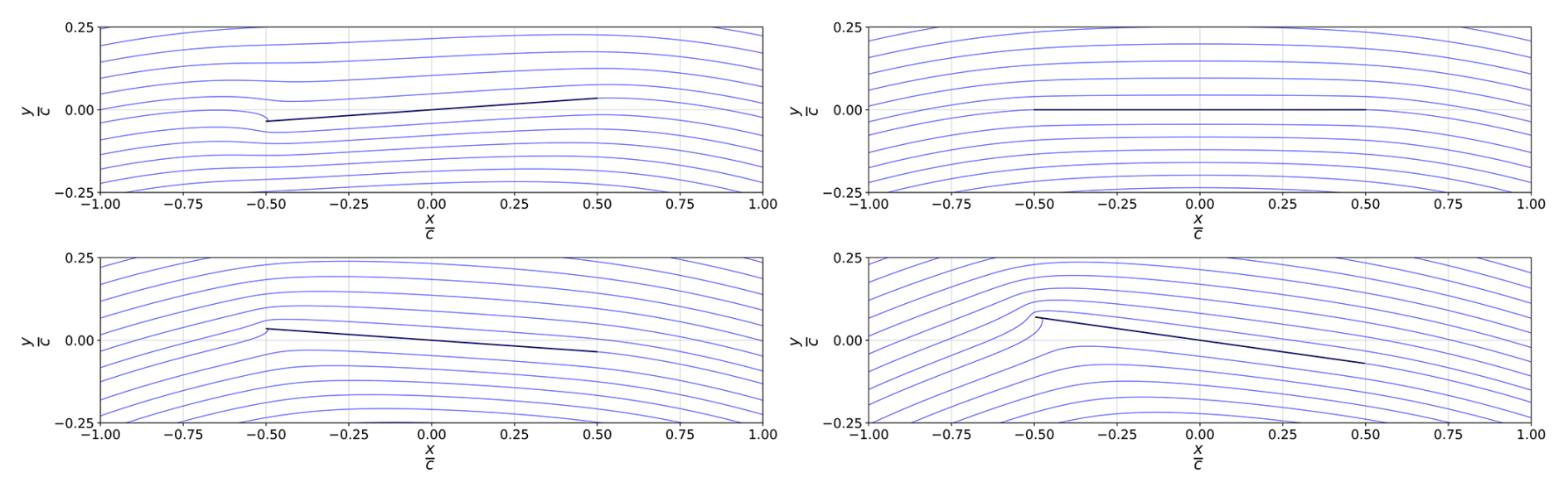
Figure 1 Streamlines (blue) of curved potential flows past a flat plate (black) with $c/R=\mathrm{2}/\mathrm{7}$ and for various tilt angles: ${\mathit{\alpha }}_{\mathrm{p}}=-\mathrm{4}$, 0, 4 and 8 °.

One can make an analogy between the potential flow and the flow past a flat plate that is attached at its center to an arm of length R that rotates at the angular velocity Ω. The upstream velocity seen by the plate is U=(Ω R) and its analog is the velocity $U=\frac{{\mathrm{\Gamma }}_{\mathrm{0}}}{\mathrm{2}\mathit{\pi }R}$ induced by the vortex in the potential flow model; this sets ${\mathrm{\Gamma }}_{\mathrm{0}}=-\mathrm{2}\mathit{\pi }\mathrm{\Omega }{R}^{\mathrm{2}}$.

However, it must be stressed that the analogy is limited. The potential flow being irrotational, the velocity induced by the vortex decreases when R increases; for the plate in solid body rotation, the velocity increases with increasing R. In particular, the analogy can only be used to obtain a model for the normal force f_n exerted by the flow on the plate and for the moment m_ac around its aerodynamic center, only for moderate tilt angles. Properly modeling the tangential force f_t will require another argument that is not compatible with potential flow theory, even for inviscid flows, and this will be developed in the paper.

When considering airfoils (thus with some thickness) instead of plates, the models for f_n and m_ac based on the analogy with potential flow will also be acceptable if all points of the airfoil remain such that their distance to the airfoil center is small compared to the arm length R.

3.2 Transformation used for developing the simplified model

The complex potential due to the vortex is

$$\begin{array}{}\text{(1)}& \begin{array}{rl}{\displaystyle }f\left(z\right)=& {\displaystyle }\mathit{\varphi }\left(z\right)+\mathrm{i}\mathit{\psi }\left(z\right)=-\mathrm{i}{\displaystyle \frac{{\mathrm{\Gamma }}_{\mathrm{0}}}{\mathrm{2}\mathit{\pi }}}\log \left({\displaystyle \frac{z+\mathrm{i}R}{R}}\right)\\ {\displaystyle }=& {\displaystyle }\mathrm{i}UR\log \left({\displaystyle \frac{z}{R}}+i\right),\end{array}\end{array}$$

with $z=x+\mathrm{i}y$ the complex variable, ϕ(z) the potential and ψ(z) the streamfunction. As it is defined up to an arbitrary constant, we can subtract $\log \left(i\right)=\mathit{\pi }/\mathrm{2}$ and also write

$$\begin{array}{}\text{(2)}& f\left(z\right)=\mathrm{i}UR\log \left(\mathrm{1}-\mathrm{i}{\displaystyle \frac{z}{R}}\right).\end{array}$$

This then leads to the conformal transformation proposed in Akimoto et al. (2013):

$$\begin{array}{}\text{(3)}& Z\left(z\right)=\mathrm{i}R\log \left(\mathrm{1}-\mathrm{i}{\displaystyle \frac{z}{R}}\right)\iff z\left(Z\right)=\mathrm{i}R\left({\mathrm{e}}^{-\mathrm{i}\frac{Z}{R}}-\mathrm{1}\right).\end{array}$$

Now, for z points with $\frac{\left|z\right|}{R}$ small, which is the case when $\frac{c/\mathrm{2}}{R}\ll \mathrm{1}$, each conformal transformation can be approximated using the first term in its Taylor series:

$$\begin{array}{}\text{(4)}& Z\left(z\right)\simeq z+{\displaystyle \frac{\mathrm{i}}{\mathrm{2}}}{\displaystyle \frac{z^{\mathrm{2}}}{R}}\iff z\left(Z\right)\simeq Z-{\displaystyle \frac{\mathrm{i}}{\mathrm{2}}}{\displaystyle \frac{Z^{\mathrm{2}}}{R}}.\end{array}$$

These simplified transformations are those retained in what follows for developing the correction models accounting for flow curvature effects.

The flat plate in the z plane is transformed into a curved plate in the Z plane, and the potential f(z) for the curved flow past the flat plate can be approximated from the potential F(Z) of a uniform flow past the cambered plate: this is done by writing f(z)=F(Z) for z=z(Z). We stress that this approximated potential flow is not the exact one; the exact one is that developed in Appendix E. Nevertheless, we will see that the analogy between the flow of a rotating airfoil attached to an arm and this simplified potential flow already allows one to model quite well the effects of flow curvature on the force normal to the arm and on the aerodynamic moment. However, the analogy completely fails to model the force tangential to the arm (and so does the exact solution of Appendix E). The proper model for the tangential force will be obtained by considering the rotating airfoil attached to an arm and the net moment at the center of rotation (which must be zero in inviscid flow).

3.3 Flat plate or thin airfoil attached at its mid-chord ($x_{\mathrm{p}}=c/\mathrm{2}$)

3.3.1 Flat plate without pitch angle in an inviscid flow

We first consider a flat plate of chord c in the z plane, which is centered at z_c=0 and is also attached to the arm there: z_p=0 (which corresponds to the case $x_{\mathrm{p}}=c/\mathrm{2}$). The plate is horizontal: no pitch angle (α_p=0): see Fig. 2a.

Using the transformation $Z\left(z\right)=z+\frac{\mathrm{i}}{\mathrm{2}}\frac{z^{\mathrm{2}}}{R}$, the plate is transformed into a horizontal and symmetric cambered plate in the Z plane: the attachment point $z_{\mathrm{p}}=z_{\mathrm{c}}=\mathrm{0}$ is transformed into $Z_{\mathrm{p}}=Z_c=\mathrm{0}$, the trailing edge $z_{\mathrm{T}}=c/\mathrm{2}$ is transformed into $Z_{\mathrm{T}}=c/\mathrm{2}+\mathrm{i}{c}^{\mathrm{2}}/\left(\mathrm{8}R\right)$ and the leading edge $z_{\mathrm{L}}=-c/\mathrm{2}$ is transformed into $Z_{\mathrm{L}}=-c/\mathrm{2}+\mathrm{i}{c}^{\mathrm{2}}/\left(\mathrm{8}R\right)$; see Fig. 2b.

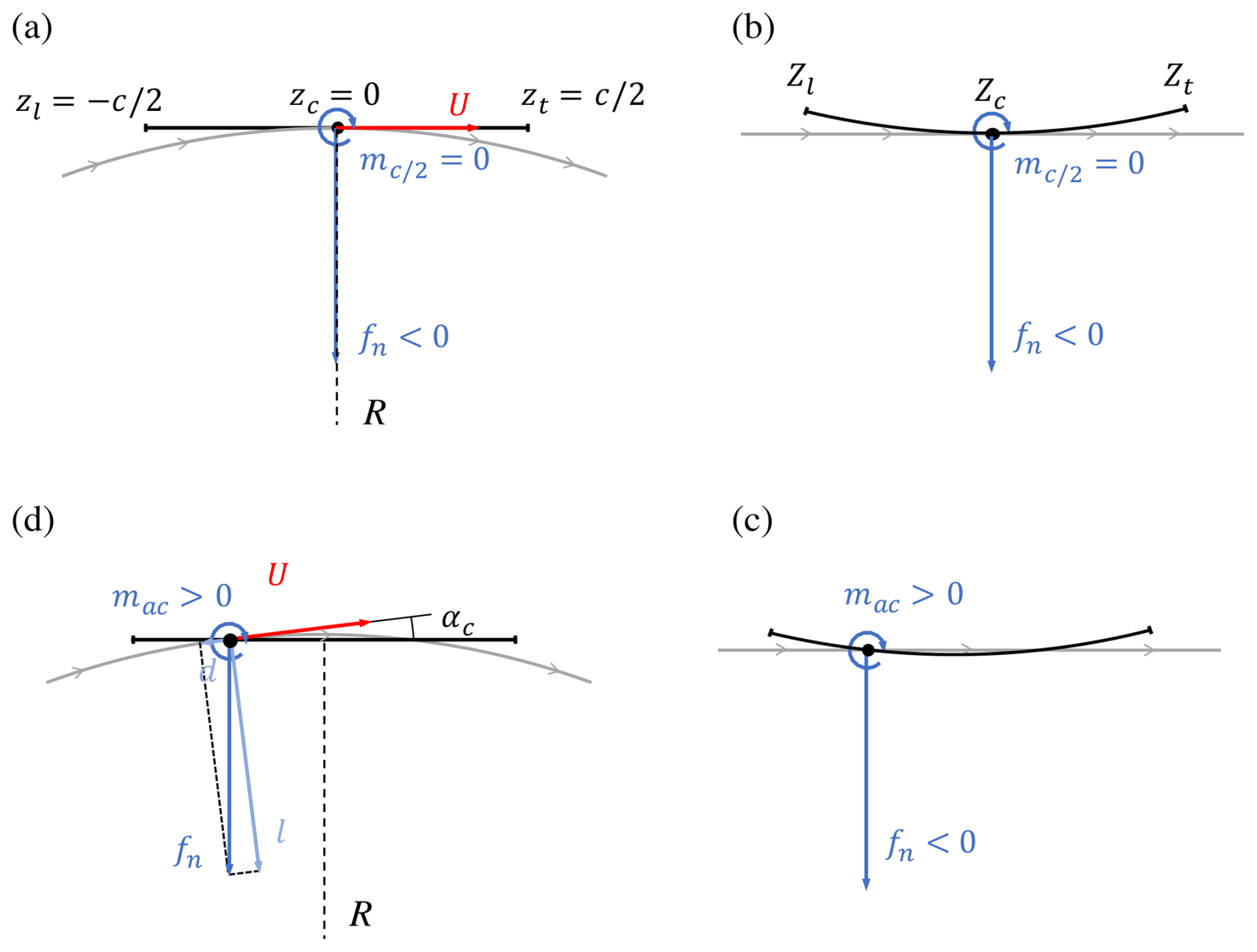
Figure 2 (a, d) Schematic of a flat plate attached at $x_{\mathrm{p}}=c/\mathrm{2}$ without pitch angle in the z plane (solid black) and a background flow with curved streamlines (light gray). (b, c) Transformed cambered plate in the Z plane in a uniform background flow. Note that the flow curvature was here exaggerated for clarity, using a too-large value of $c/R=\mathrm{1}/\mathrm{2}$.

Using the approximate potential flow discussed above, the normal force, f_n, exerted by the flow U on the cambered plate is obtained as

$$\begin{array}{}\text{(5)}& C_{\mathrm{n}}\left(\mathrm{0}\right)=-\mathrm{2}\mathit{\pi }{\displaystyle \frac{c}{\mathrm{4}R}}.\end{array}$$

The force f_n(0) is negative, thus oriented inward.

On the other hand, we also have the exact value of C_n(0) obtained from the exact potential flow presented in Appendix E, with the final result of Eq. (E25). The amplitude of C_n(0) is thus a little bit less than $\mathrm{2}\mathit{\pi }\frac{c}{\mathrm{4}R}$. Nevertheless: when ${\left(\frac{c}{\mathrm{2}R}\right)}^{\mathrm{2}}\ll \mathrm{1}$, which is most often the case and is the one considered in this paper, we can neglect this effect. We then simply associate the flow curvature effect with an effective shift in the angle of attack, by the angle α_c defined as

$$\begin{array}{}\text{(6)}& \sin \left({\mathit{\alpha }}_{\mathrm{c}}\right)={\displaystyle \frac{c}{\mathrm{4}R}}\Rightarrow C_{\mathrm{n}}\left(\mathrm{0}\right)=-\mathrm{2}\mathit{\pi }\sin \left({\mathit{\alpha }}_{\mathrm{c}}\right).\end{array}$$

The aerodynamic moment $m_{c/\mathrm{2}}\left(\mathrm{0}\right)$ acting at the center of the plate (i.e.,  at the mid-chord point) is here zero, by left–right symmetry of the flow around the plate, in the same way as for the potential flow developed in Appendix E and shown in Fig. 1.

For an inviscid flow, it would take no energy to rotate the airfoil attached to the arm: the moment m₀ around the center of rotation of the arm would therefore be zero. We stress that this is also confirmed in Appendix D by performing an inviscid simulation of the flow past a rotating airfoil. As this moment is equal to $m_{\mathrm{0}}=m_{c/\mathrm{2}}\left(\mathrm{0}\right)+R{f}_{\mathrm{t}}\left(\mathrm{0}\right)$, and since $m_{c/\mathrm{2}}\left(\mathrm{0}\right)=\mathrm{0}$, the tangential force exerted on the plate by an inviscid flow will also be zero: f_t(0)=0 and hence C_t(0)=0. For a viscous flow, there will, of course, be some parasitic drag, and thus a value of C_t(0)>0; we will add this effect later, in Sect. 3.3.3.

We already stress that, in an inviscid flow, the tangential force will no longer be zero when the plate is pitched by some angle α_p, because $m_{c/\mathrm{2}}$ will then be non-zero; see Sect. 3.3.2.

We also obtain the moment at the location of the aerodynamic center (which is located at a distance $c/\mathrm{4}$ from the leading edge): since $m_{c/\mathrm{2}}\left(\mathrm{0}\right)=\mathrm{0}$, we obtain $m_{\text{ac}}\left(\mathrm{0}\right)=m_{c/\mathrm{4}}\left(\mathrm{0}\right)=-(c/\mathrm{4})f_{\mathrm{n}}\left(\mathrm{0}\right)>\mathrm{0}$; see Fig. 2c and d. The associated moment coefficient is thus

$$\begin{array}{}\text{(7)}& \begin{array}{rl}{\displaystyle }{C}_{m_{\text{ac}}}\left(\mathrm{0}\right)=& {\displaystyle }{C}_{m_{c/\mathrm{4}}}\left(\mathrm{0}\right)={\displaystyle \frac{m_{c/\mathrm{4}}\left(\mathrm{0}\right)}{\frac{\mathrm{1}}{\mathrm{2}}\mathit{\rho }{U}^{\mathrm{2}}{c}^{\mathrm{2}}}}\\ {\displaystyle }=& {\displaystyle }-{\displaystyle \frac{C_{\mathrm{n}}\left(\mathrm{0}\right)}{\mathrm{4}}}\simeq {\displaystyle \frac{\mathit{\pi }}{\mathrm{2}}}\sin \left({\mathit{\alpha }}_{\mathrm{c}}\right)\simeq {\displaystyle \frac{\mathit{\pi }}{\mathrm{2}}}{\displaystyle \frac{c}{\mathrm{4}R}}.\end{array}\end{array}$$

We note that the angle α_p=0 considered here is the geometrical pitch angle of the profile attached at its mid-point relatively to the horizontal, not the angle that the profile makes with the curved flow streamline at the location of the aerodynamic center and which is used as the “effective angle of attack” α in an actuator line method (ALM) when the line is located at the aerodynamic center. At this location, the curved streamline makes an angle of $\mathit{\alpha }=\frac{c}{\mathrm{4}R}$ relative to the horizontal plate (see Fig. 2d); thus an angle also equal to α_c.

The usual aerodynamic coefficients relative to the curved flow velocity vector considered at the location of the aerodynamic center are easily obtained using the angle α_c of the local velocity vector relative to the plate:

$$\begin{array}{}\text{(8)}& \begin{array}{rl}{\displaystyle }{C}_{\mathrm{l}}=& {\displaystyle }{C}_{\mathrm{n}}\left(\mathrm{0}\right)\cos \left({\mathit{\alpha }}_{\mathrm{c}}\right),\\ {\displaystyle }{C}_{\mathrm{d}}=& {\displaystyle }{C}_{\mathrm{n}}\left(\mathrm{0}\right)\sin \left({\mathit{\alpha }}_{\mathrm{c}}\right).\end{array}\end{array}$$

As C_n(0) is negative, both C_l and C_d are negative; as shown in Fig. 2d.

3.3.2 Flat plate with pitch angle in an inviscid flow

We now further pitch the flat plate at a moderate angle α_p relative to the horizontal, as shown in Fig. 3a. The normal force coefficient will be modeled using

$$\begin{array}{}\text{(9)}& C_{\mathrm{n}}\left({\mathit{\alpha }}_{\mathrm{p}}\right)\simeq \mathrm{2}\mathit{\pi }\sin \left({\mathit{\alpha }}_{\mathrm{p}}\right)-\mathrm{2}\mathit{\pi }\sin \left({\mathit{\alpha }}_{\mathrm{c}}\right).\end{array}$$

We note that this formula is slightly different from the formula inspired from the potential flow theory past a cambered plate, which would be

$$\begin{array}{}\text{(10)}& C_{\mathrm{n}}\left({\mathit{\alpha }}_{\mathrm{p}}\right)\simeq \mathrm{2}\mathit{\pi }\sin ({\mathit{\alpha }}_{\mathrm{p}}-{\mathit{\alpha }}_{\mathrm{c}}).\end{array}$$

Obviously, both formulas provide results that are very close for small α_c and moderate α_p−α_c; they both also provide C_n=0 when α_p=α_c. The reason why we will use Eq. (9) instead of Eq. (10) will become clear when we further extend the model to thin airfoils in real viscous flows and up to large pitch angles, even up to the stall of the airfoil, and compare the results to those of the reference CFD results.

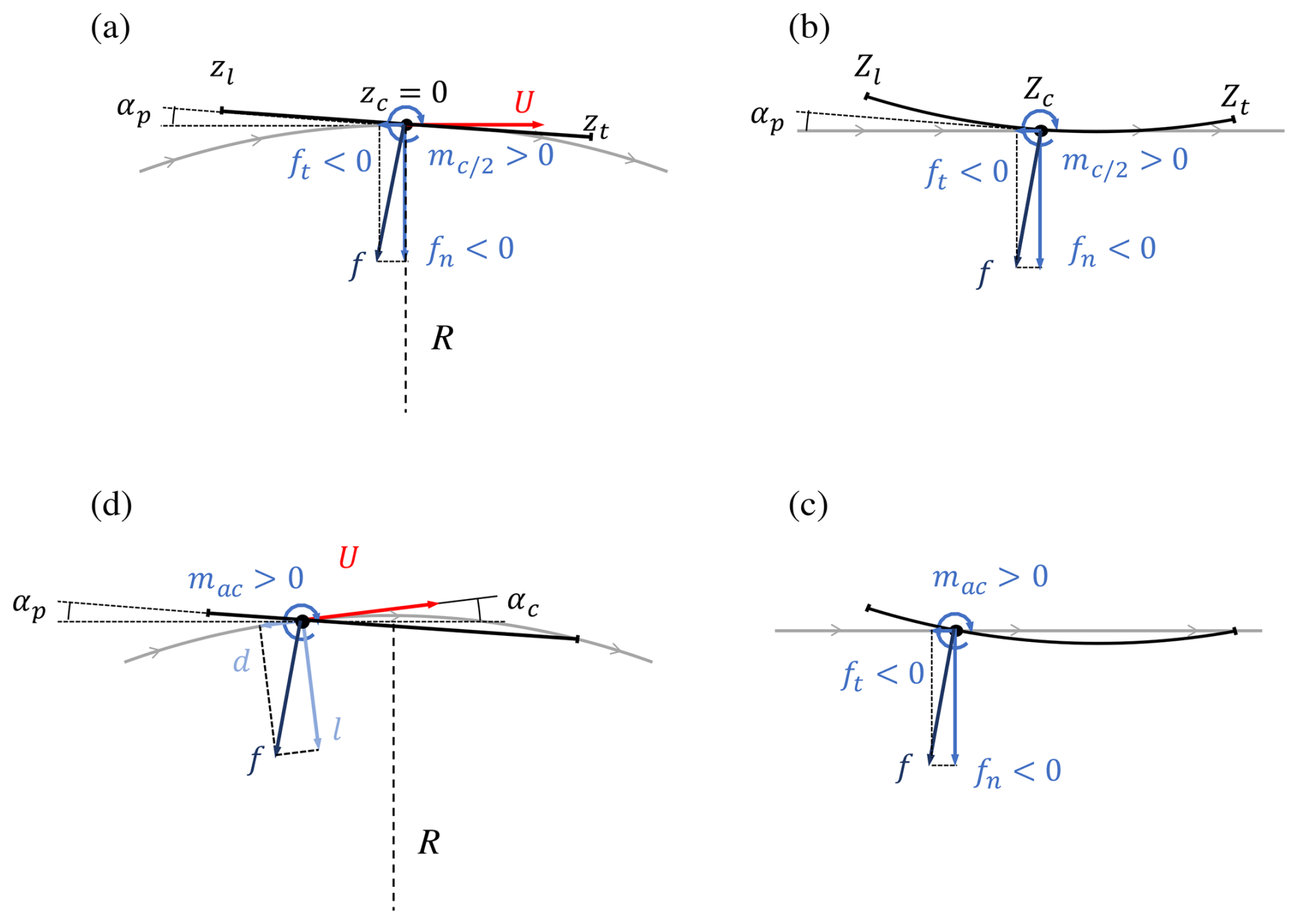
Figure 3 (a, d) Schematic of a flat plate attached at $x_{\mathrm{p}}=c/\mathrm{2}$ with a moderate pitch angle $\mathrm{0}<{\mathit{\alpha }}_{\mathrm{p}}<{\mathit{\alpha }}_{\mathrm{c}}$ in the z plane (solid black) and a background flow with curved streamlines (light gray). (b, c) Transformed tilted cambered plate in the Z plane in a uniform background flow. Note that the flow curvature was here exaggerated for clarity, using a too-large value of $c/R=\mathrm{1}/\mathrm{2}$.

For α_p<α_c, C_n<0 and the normal force is oriented inward, as in Fig. 3a; for α_p>α_c, C_n>0 and the normal force is oriented outward.

When α_p≠0, the flow around the plate is no longer left-right symmetric (as for the potential flow shown in Fig. 1). The moment $m_{c/\mathrm{2}}$ around the center of the plate is, therefore, non-zero.

For the model, we use the prediction for a potential flow past the tilted cambered plate put in an horizontal stream at velocity U:

$$\begin{array}{}\text{(11)}& \begin{array}{rl}{\displaystyle }{C}_{m_{c/\mathrm{2}}}\left({\mathit{\alpha }}_{\mathrm{p}}\right)=& {\displaystyle \frac{m_{c/\mathrm{2}}}{\frac{\mathrm{1}}{\mathrm{2}}\mathit{\rho }{U}^{\mathrm{2}}{c}^{\mathrm{2}}}}={\displaystyle \frac{\mathit{\pi }}{\mathrm{4}}}\sin \left(\mathrm{2}{\mathit{\alpha }}_{\mathrm{p}}\right)\\ {\displaystyle }=& {\displaystyle \frac{\mathit{\pi }}{\mathrm{2}}}\sin \left({\mathit{\alpha }}_{\mathrm{p}}\right)\cos \left({\mathit{\alpha }}_{\mathrm{p}}\right).\end{array}\end{array}$$

The moment around the aerodynamic center is hence obtained as $m_{c/\mathrm{4}}\left({\mathit{\alpha }}_{\mathrm{p}}\right)=m_{c/\mathrm{2}}\left({\mathit{\alpha }}_{\mathrm{p}}\right)-\left(\cos \right({\mathit{\alpha }}_{\mathrm{p}})c/\mathrm{4})f_{\mathrm{n}}\left({\mathit{\alpha }}_{\mathrm{p}}\right)$, and thus the associated moment coefficient is

$$\begin{array}{}\text{(12)}& \begin{array}{rl}{\displaystyle }{C}_{m_{c/\mathrm{4}}}\left({\mathit{\alpha }}_{\mathrm{p}}\right)=& {\displaystyle }{C}_{m_{c/\mathrm{2}}}\left({\mathit{\alpha }}_{\mathrm{p}}\right)-{\displaystyle \frac{C_{\mathrm{n}}\left({\mathit{\alpha }}_{\mathrm{p}}\right)}{\mathrm{4}}}\cos \left({\mathit{\alpha }}_{\mathrm{p}}\right)\\ {\displaystyle }\simeq & {\displaystyle \frac{\mathit{\pi }}{\mathrm{2}}}\sin \left({\mathit{\alpha }}_{\mathrm{c}}\right)\cos \left({\mathit{\alpha }}_{\mathrm{p}}\right).\end{array}\end{array}$$

As the moment m₀ around the center of rotation of the arm must still be zero in an inviscid flow (see also Appendix D for a numerical confirmation of this), there must now also be a net tangential force component $f_{\mathrm{t}}^{\mathrm{i}}$ due solely to the pressure distribution, and which is such that

$$\begin{array}{}\text{(13)}& m_{\mathrm{0}}=m_{c/\mathrm{2}}\left({\mathit{\alpha }}_{\mathrm{p}}\right)+R{f}_{\mathrm{t}}^{\mathrm{i}}\left({\mathit{\alpha }}_{\mathrm{p}}\right)=\mathrm{0}.\end{array}$$

The model for the tangential force coefficient in inviscid flow is hence obtained as

$$\begin{array}{}\text{(14)}& C_{\mathrm{t}}^{\mathrm{i}}\left({\mathit{\alpha }}_{\mathrm{p}}\right)=-{\displaystyle \frac{c}{R}}{C}_{m_{c/\mathrm{2}}}\left({\mathit{\alpha }}_{\mathrm{p}}\right)\simeq -\mathrm{4}\sin \left({\mathit{\alpha }}_{\mathrm{c}}\right)C_{m_{c/\mathrm{2}}}\left({\mathit{\alpha }}_{\mathrm{p}}\right).\end{array}$$

Of course, there will also be a parasitic drag coefficient to add to the model for C_t when modeling viscous flow; see Sect. 3.3.3.

3.3.3 Thin airfoil with pitch angle in a real viscous flow

The correction models above, obtained assuming an inviscid flow and a flat plate, are also used for thin aerodynamic profiles without camber and in real flows and thus with the added parasitic effects associated with viscosity.

For the normal force coefficient, the model becomes

$$\begin{array}{}\text{(15)}& C_{\mathrm{n}}\left({\mathit{\alpha }}_{\mathrm{p}}\right)\simeq C_{\mathrm{l}}^{\mathrm{u}}\left({\mathit{\alpha }}_{\mathrm{p}}\right)-C_{\mathrm{l}}^{\mathrm{u}}\left({\mathit{\alpha }}_{\mathrm{c}}\right),\end{array}$$

where $C_{\mathrm{l}}^{\mathrm{u}}\left(\mathit{\beta }\right)$ is the usual curve for the lift coefficient of the airfoil in a uniform flow as a function of its angle of attack β relative to that uniform flow. This curve is obtained from experiments or using CFD. In the present case, it was obtained using CFD; see Appendix A.

When the airfoil is not pitched, the moment at mid-chord, $C_{m_{c/\mathrm{2}}}^{\mathrm{0}}$, is small yet non-zero. It can be estimated by performing CFD of the airfoil deformed using the transformation Z(z) and put in a uniform flow (for the deformed NACA0015 airfoil, we measure $C_{m_{c/\mathrm{2}}}^{\mathrm{0}}\simeq -\mathrm{0.00746}$: see Appendix C).

When the airfoil is pitched by an angle α_p, we then use, by similarity with the model obtained for the plate,

$$\begin{array}{}\text{(16)}& C_{m_{c/\mathrm{2}}}\left({\mathit{\alpha }}_{\mathrm{p}}\right)\simeq C_{m_{c/\mathrm{2}}}^{\mathrm{0}}+{\displaystyle \frac{\mathrm{1}}{\mathrm{4}}}{C}_{\mathrm{l}}^{\mathrm{u}}\left({\mathit{\alpha }}_{\mathrm{p}}\right)\cos \left({\mathit{\alpha }}_{\mathrm{p}}\right).\end{array}$$

We then obtain, for the moment around the quarter-chord point,

$$\begin{array}{}\text{(17)}& \begin{array}{rl}{\displaystyle }{C}_{m_{c/\mathrm{4}}}\left({\mathit{\alpha }}_{\mathrm{p}}\right)=& {\displaystyle }{C}_{m_{c/\mathrm{2}}}\left({\mathit{\alpha }}_{\mathrm{p}}\right)-{\displaystyle \frac{\mathrm{1}}{\mathrm{4}}}{C}_{\mathrm{n}}\left({\mathit{\alpha }}_{\mathrm{p}}\right)\cos \left({\mathit{\alpha }}_{\mathrm{p}}\right)\\ {\displaystyle }\simeq & {\displaystyle }{C}_{m_{c/\mathrm{2}}}^{\mathrm{0}}+{\displaystyle \frac{\mathrm{1}}{\mathrm{4}}}{C}_{\mathrm{l}}^{\mathrm{u}}\left({\mathit{\alpha }}_{\mathrm{c}}\right)\cos \left({\mathit{\alpha }}_{\mathrm{p}}\right).\end{array}\end{array}$$

In the same way, the moment around the true aerodynamic center, which is located at $\frac{x_{\text{ac}}}{c}$ very close to $\frac{\mathrm{1}}{\mathrm{4}}$ but not exactly there (for the NACA0015 airfoil, we measure $\frac{x_{\text{ac}}}{c}\simeq \mathrm{0.2476}$: see Appendix A), is obtained as

$$\begin{array}{}\text{(18)}& C_{m_{\text{ac}}}\left({\mathit{\alpha }}_{\mathrm{p}}\right)\simeq C_{m_{c/\mathrm{2}}}^{\mathrm{0}}+\left({\displaystyle \frac{\mathrm{1}}{\mathrm{2}}}-{\displaystyle \frac{x_{\text{ac}}}{c}}\right)C_{\mathrm{l}}^{\mathrm{u}}\left({\mathit{\alpha }}_{\mathrm{c}}\right)\cos \left({\mathit{\alpha }}_{\mathrm{p}}\right).\end{array}$$

To model the tangential force coefficient C_t, we add to the inviscid flow contribution, $C_{\mathrm{t}}^{\mathrm{i}}=-\frac{c}{R}{C}_{m_{c/\mathrm{2}}}$, the parasitic contribution $C_{\mathrm{t}}^{\mathit{\nu }}$ associated with the viscous effects, i.e., due to the presence of boundary layers and their separation, resulting in pressure drag and friction drag:

$$\begin{array}{}\text{(19)}& \begin{array}{rl}{\displaystyle }{C}_{\mathrm{t}}\left({\mathit{\alpha }}_{\mathrm{p}}\right)=& {\displaystyle }{C}_{\mathrm{t}}^{\mathit{\nu }}\left({\mathit{\alpha }}_{\mathrm{p}}\right)+C_{\mathrm{t}}^{\mathrm{i}}\left({\mathit{\alpha }}_{\mathrm{p}}\right)\\ {\displaystyle }=& {\displaystyle }\left(C_{\mathrm{t}}^{\mathit{\nu },\mathrm{p}}\left({\mathit{\alpha }}_{\mathrm{p}}\right)+C_{\mathrm{t}}^{\mathrm{i}}\left({\mathit{\alpha }}_{\mathrm{p}}\right)\right)+C_{\mathrm{t}}^{\mathit{\nu },\mathrm{f}}\left({\mathit{\alpha }}_{\mathrm{p}}\right)\\ {\displaystyle }=& {\displaystyle }{C}_{\mathrm{t}}^{\mathrm{p}}\left({\mathit{\alpha }}_{\mathrm{p}}\right)+C_{\mathrm{t}}^{\mathit{\nu },\mathrm{f}}\left({\mathit{\alpha }}_{\mathrm{p}}\right)\\ {\displaystyle }\simeq & {\displaystyle }\left(C_{\mathrm{d}}^{\text{u,p}}\left({\mathit{\alpha }}_{\mathrm{p}}\right)-{\displaystyle \frac{c}{R}}{C}_{m_{c/\mathrm{2}}}\left({\mathit{\alpha }}_{\mathrm{p}}\right)\right)+C_{\mathrm{d}}^{\text{u,f}}({\mathit{\alpha }}_{\mathrm{p}}+{\mathit{\alpha }}_{\mathrm{c}}).\end{array}\end{array}$$

The term $C_{\mathrm{t}}^{\mathit{\nu },\mathrm{p}}+C_{\mathrm{t}}^{\mathrm{i}}$ in parentheses represents the complete pressure component: we denote it $C_{\mathrm{t}}^{\mathrm{p}}$.

Note that we modeled $C_{\mathrm{t}}^{\mathit{\nu },\mathrm{f}}\left({\mathit{\alpha }}_{\mathrm{p}}\right)$ using $C_{\mathrm{d}}^{\text{u,f}}({\mathit{\alpha }}_{\mathrm{p}}+{\mathit{\alpha }}_{\mathrm{c}})$ with $C_{\mathrm{d}}^{\text{u,f}}\left(\mathit{\beta }\right)$ the curve for the fraction due to wall friction of the drag coefficient for the airfoil in uniform flow as a function of its angle of attack β (see Appendix A). This choice is motivated by the fact that, in the reference CFD of the rotating airfoil, $C_{\mathrm{t}}^{\mathit{\nu },\mathrm{f}}$ is seen to be minimum when ${\mathit{\alpha }}_{\mathrm{p}}\simeq -{\mathit{\alpha }}_{\mathrm{c}}$ and not when α_p≃0. As to $C_{\mathrm{t}}^{\mathrm{p}}=C_{\mathrm{t}}^{\mathit{\nu },\mathrm{p}}+C_{\mathrm{t}}^{\mathrm{i}}$, it is found, in the CFD, to be symmetric relative to α_p≃0, and hence we model $C_{\mathrm{t}}^{\mathit{\nu },\mathrm{p}}\left({\mathit{\alpha }}_{\mathrm{p}}\right)$ using $C_{\mathrm{d}}^{\text{u,p}}\left({\mathit{\alpha }}_{\mathrm{p}}\right)$. The model for the parasitic drag is thus taken as

$$\begin{array}{}\text{(20)}& \begin{array}{rl}{\displaystyle }{C}_{\mathrm{t}}^{\mathit{\nu }}\left({\mathit{\alpha }}_{\mathrm{p}}\right)=& {\displaystyle }{C}_{\mathrm{t}}^{\mathit{\nu },\mathrm{p}}\left({\mathit{\alpha }}_{\mathrm{p}}\right)+C_{\mathrm{t}}^{\mathit{\nu },\mathrm{f}}\left({\mathit{\alpha }}_{\mathrm{p}}\right)\\ {\displaystyle }\simeq & {\displaystyle }{C}_{\mathrm{d}}^{\text{u,p}}\left({\mathit{\alpha }}_{\mathrm{p}}\right)+C_{\mathrm{d}}^{\text{u,f}}({\mathit{\alpha }}_{\mathrm{p}}+{\mathit{\alpha }}_{\mathrm{c}}).\end{array}\end{array}$$

We also stress an important point: if the moment $m_{c/\mathrm{2}}$ is not enforced in the ALM (using the procedure developed in Sect. 5), then only the parasitic tangential force $f_{\mathrm{t}}^{\mathit{\nu }}$ must be enforced in the ALM, while $f_{\mathrm{t}}^{\mathrm{i}}$ must be ignored.

Finally, the force coefficients can also be decomposed into the usual aerodynamic coefficients considered at $c/\mathrm{4}$ by using the angle of attack α_p+α_c that the curved flow velocity vector makes there relative to the airfoil chord:

$$\begin{array}{}\text{(21)}& \begin{array}{rl}{\displaystyle }{C}_{\mathrm{l}}=& {\displaystyle }{C}_{\mathrm{n}}\left({\mathit{\alpha }}_{\mathrm{p}}\right)\cos \left({\mathit{\alpha }}_{\mathrm{c}}\right)-C_{\mathrm{t}}\left({\mathit{\alpha }}_{\mathrm{p}}\right)\sin \left({\mathit{\alpha }}_{\mathrm{c}}\right),\\ {\displaystyle }{C}_{\mathrm{d}}=& {\displaystyle }{C}_{\mathrm{n}}\left({\mathit{\alpha }}_{\mathrm{p}}\right)\sin \left({\mathit{\alpha }}_{\mathrm{c}}\right)+C_{\mathrm{t}}\left({\mathit{\alpha }}_{\mathrm{p}}\right)\cos \left({\mathit{\alpha }}_{\mathrm{c}}\right).\end{array}\end{array}$$

3.3.4 Comparison of the model predictions against CFD data of a rotating NACA0015 airfoil

We test the curvature correction models proposed above for a case with significant curvature effects (with $c/R=\mathrm{2}/\mathrm{7}$) and for a NACA0015 airfoil (hence an airfoil that is not very thin) attached at $x_{\mathrm{p}}=c/\mathrm{2}$. We then obtain $\sin \left({\mathit{\alpha }}_{\mathrm{c}}\right)=\mathrm{1}/\mathrm{14}\simeq \mathrm{0.07143}$ and ${\mathit{\alpha }}_{\mathrm{c}}=\arcsin (\mathrm{1}/\mathrm{14})\simeq \mathrm{0.07149}\mathrm{rad}$ (thus ≃4.096 °).

We first consider the case α_p=0. Using the lift curve of the NACA0015, the prediction is $C_{\mathrm{n}}\simeq -C_{\mathrm{l}}^{\mathrm{u}}\left({\mathit{\alpha }}_{\mathrm{c}}\right)\simeq -\mathrm{0.454}$ ($C_{\mathrm{n}}\simeq -\mathrm{2}\mathit{\pi }(\mathrm{1}/\mathrm{14})\simeq -\mathrm{0.449}$ when using the flat plate model) to compare with $C_{\mathrm{n}}\simeq -\mathrm{0.431}$ measured in CFD of the rotating airfoil.

For the flat plate, we have $C_{m_{c/\mathrm{2}}}=\mathrm{0}$ and thus $C_{m_{c/\mathrm{4}}}=C_{m_{\text{ac}}}=-C_{\mathrm{n}}/\mathrm{4}\simeq (\mathit{\pi }/\mathrm{2})(\mathrm{1}/\mathrm{14})\simeq \mathrm{0.1122}$. For the NACA0015 airfoil, and if $C_{m_{c/\mathrm{2}}}^{\mathrm{0}}$ is neglected, the predictions are $C_{m_{c/\mathrm{4}}}\simeq \mathrm{0.1135}$ and $C_{m_{\text{ac}}}\simeq \mathrm{0.1146}$. The values measured in CFD of the rotating airfoil are $C_{m_{c/\mathrm{2}}}\simeq -\mathrm{0.0056}$, $C_{m_{c/\mathrm{4}}}\simeq \mathrm{0.10225}$ and $C_{m_{\text{ac}}}\simeq \mathrm{0.10327}$. When using the modeled $C_{m_{c/\mathrm{2}}}^{\mathrm{0}}\simeq -\mathrm{0.00746}$ (obtained using CFD of the airfoil deformed using Z(z) and put in a uniform flow; see Appendix C), the predictions are $C_{m_{c/\mathrm{4}}}\simeq \mathrm{0.1079}$ and $C_{m_{\text{ac}}}\simeq \mathrm{0.1090}$: indeed better.

The values measured in CFD of the rotating airfoil are also $C_{\mathrm{t}}^{\mathrm{p}}\simeq \mathrm{0.00387}$, $C_{\mathrm{t}}^{\mathit{\nu },\mathrm{f}}\simeq \mathrm{0.00682}$ and thus C_t≃0.01069. When using the modeled $C_{m_{c/\mathrm{2}}}^{\mathrm{0}}$ value, the predictions become $C_{\mathrm{t}}^{\mathrm{i}}\simeq \mathrm{0.00211}$ and thus $C_{\mathrm{t}}^{\mathrm{p}}\simeq \mathrm{0.00401}$, which compares well with the reference CFD value. The model is again improved when we incorporate the small, yet non-zero, value of $C_{m_{c/\mathrm{2}}}^{\mathrm{0}}$.

We present in Fig. 4 the predicted values for the aerodynamic coefficients. The range of moderate pitch angles corresponds to $-\mathrm{12}\le {\mathit{\alpha }}_{\mathrm{p}}\le \mathrm{12}\mathit{°}$. We see that the predictions are quite accurate within this range. The comparison is also made for the complete range, up to the two stall angles (they are slightly different due to the flow curvature effects). We see that the model developed above also performs well up to both stall angles and that the predicted values (of roughly −18 ° and 18 °) are in fair agreement with those of the reference CFD (that are roughly −19 ° and 17 deg). We stress that this would not be the case if we had used

$$\begin{array}{}\text{(22)}& C_{\mathrm{n}}\left({\mathit{\alpha }}_{\mathrm{p}}\right)\simeq C_{\mathrm{l}}^{\mathrm{u}}({\mathit{\alpha }}_{\mathrm{p}}-{\mathit{\alpha }}_{\mathrm{c}}),\end{array}$$

as model for C_n instead of Eq. (15). Although both choices produce similar predictions for C_n, and hence also for all other coefficients, in the range of moderate tilt angles, using Eq. (22) would predict incorrect stall angles (at roughly $-\mathrm{18}+\mathrm{4}=-\mathrm{14}\mathit{°}$ and $\mathrm{18}+\mathrm{4}=\mathrm{22}\mathit{°}$: not in line with those of the reference CFD).

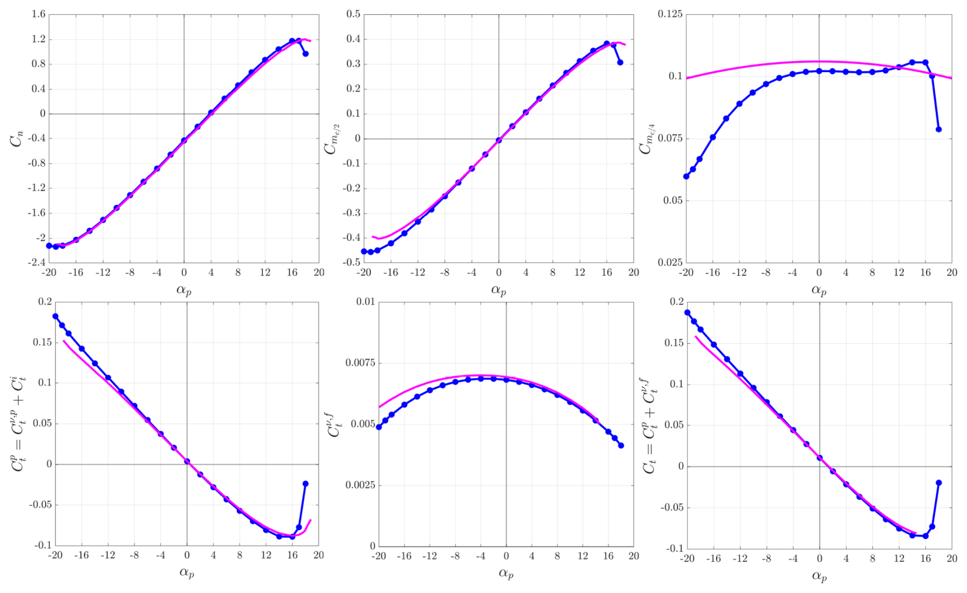
Figure 4 NACA0015 airfoil in rotation with $c/R=\mathrm{2}/\mathrm{7}$ and attached at $x_{\mathrm{p}}=c/\mathrm{2}$: comparison between the model-predicted values (magenta) of C_n, $C_{m_{c/\mathrm{2}}}$, $C_{m_{c/\mathrm{4}}}$, $C_{\mathrm{t}}^{\mathrm{p}}$, $C_{\mathrm{t}}^{\mathit{\nu },\mathrm{f}}$, C_t and the reference values obtained in CFD of the rotating airfoil (blue).

Finally, we stress that the model for $C_{m_{c/\mathrm{4}}}$ is based on the analogy of the inviscid potential flow as a cambered airfoil. As such, it cannot take into account deviations from when the pitch angle exceeds ≃10 °, where viscous effects on the moment also become significant, resulting in deviations up to $\simeq \mathrm{0.025}-\mathrm{0.03}$ near stall.

3.4 Flat plate or thin airfoil attached at its quarter-chord ($x_{\mathrm{p}}=c/\mathrm{4}$)

We consider next a flat plate of chord c in the z plane, which is attached to the arm at z_p=0 but has its center at $z_{\mathrm{c}}=c/\mathrm{4}$ (it corresponds to the case $x_{\mathrm{p}}=c/\mathrm{4}$). The plate is attached at its aerodynamic center, hence its pitch angle α_p is also the angle that the plate makes relative to the curved flow velocity vector at its aerodynamic center.

We first consider the case without pitch angle: α_p=0. The horizontal plate is transformed into a tilted and cambered plate in the Z plane: its attachment point z_p=0 is transformed into Z_p=0, its center $z_{\mathrm{c}}=c/\mathrm{4}$ is transformed into $c/\mathrm{4}+\mathrm{i}{c}^{\mathrm{2}}/\left(\mathrm{32}R\right)$, its trailing edge $z_{\mathrm{T}}=\mathrm{3}c/\mathrm{4}$ is transformed into $Z_{\mathrm{T}}=\mathrm{3}c/\mathrm{4}+\mathrm{i}\mathrm{9}{c}^{\mathrm{2}}/\left(\mathrm{32}R\right)$ and its leading edge $z_{\mathrm{L}}=-c/\mathrm{4}$ is transformed into $Z_{\mathrm{L}}=-c/\mathrm{4}+\mathrm{i}{c}^{\mathrm{2}}/\left(\mathrm{32}R\right)$; see Fig. 5.

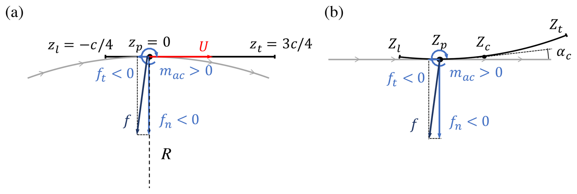
Figure 5 (a) Schematic of a flat plate attached at $x_{\mathrm{p}}=c/\mathrm{4}$ and without pitch angle in the z plane (solid black) and a background flow with curved streamlines (light gray). (b) Transformed tilted cambered plate in the Z plane in a uniform background flow. Note that the flow curvature was here exaggerated for clarity, using a too-large value of $c/R=\mathrm{1}/\mathrm{2}$.

The slope of the tilted cambered plate at its center is then obtained as $(\mathrm{d}Y/\mathrm{d}X{)}_c=c/(\mathrm{4}R)$. This is the angle that the cambered plate makes relative to the uniform horizontal velocity U. We note that this angle also corresponds to α_c.

When α_p=0, the normal force coefficient is obtained as

$$\begin{array}{}\text{(23)}& C_{\mathrm{n}}\left(\mathrm{0}\right)\simeq \mathrm{2}\mathit{\pi }\sin (\mathrm{0}-{\mathit{\alpha }}_{\mathrm{c}})-\mathrm{2}\mathit{\pi }\sin \left({\mathit{\alpha }}_{\mathrm{c}}\right)=-\mathrm{4}\mathit{\pi }\sin \left({\mathit{\alpha }}_{\mathrm{c}}\right).\end{array}$$

When we pitch the flat plate by an angle of attack α_p, the model becomes

$$\begin{array}{}\text{(24)}& C_{\mathrm{n}}\left({\mathit{\alpha }}_{\mathrm{p}}\right)\simeq \mathrm{2}\mathit{\pi }\sin ({\mathit{\alpha }}_{\mathrm{p}}-{\mathit{\alpha }}_{\mathrm{c}})-\mathrm{2}\mathit{\pi }\sin \left({\mathit{\alpha }}_{\mathrm{c}}\right).\end{array}$$

We stress again that this formula is not exactly that obtained from the potential flow theory for the curved plate in uniform flow and pitched by the angle −α_c and which would be

$$\begin{array}{}\text{(25)}& C_{\mathrm{n}}\left({\mathit{\alpha }}_{\mathrm{p}}\right)\simeq \mathrm{2}\mathit{\pi }\sin ({\mathit{\alpha }}_{\mathrm{p}}-\mathrm{2}{\mathit{\alpha }}_{\mathrm{c}}).\end{array}$$

Both formulas provide results that are very close for moderate angles. The reason why we use Eq. (24) instead of Eq. (25) is again that it provides better results when we extend the model to thin airfoils in viscous flows and up to large angles, including stall, as will be shown in the next section.

The moment coefficient at the plate center is again obtained using the angle of attack α_p−α_c of the cambered plate in the uniform flow:

$$\begin{array}{}\text{(26)}& \begin{array}{rl}{\displaystyle }{C}_{m_{c/\mathrm{2}}}\left({\mathit{\alpha }}_{\mathrm{p}}\right)=& {\displaystyle \frac{\mathit{\pi }}{\mathrm{4}}}\sin \left(\mathrm{2}\right({\mathit{\alpha }}_{\mathrm{p}}-{\mathit{\alpha }}_{\mathrm{c}}\left)\right)\\ {\displaystyle }=& {\displaystyle \frac{\mathit{\pi }}{\mathrm{2}}}\sin ({\mathit{\alpha }}_{\mathrm{p}}-{\mathit{\alpha }}_{\mathrm{c}})\cos ({\mathit{\alpha }}_{\mathrm{p}}-{\mathit{\alpha }}_{\mathrm{c}}).\end{array}\end{array}$$

This moment is indeed zero, as it should be, when α_p=α_c, as the cambered plate of the transformed flow is then horizontal. The moment coefficient around the aerodynamic center is hence also obtained as

$$\begin{array}{}\text{(27)}& \begin{array}{rl}{\displaystyle }{C}_{m_{c/\mathrm{4}}}\left({\mathit{\alpha }}_{\mathrm{p}}\right)=& {\displaystyle }{C}_{m_{c/\mathrm{2}}}\left({\mathit{\alpha }}_{\mathrm{p}}\right)-{\displaystyle \frac{C_{\mathrm{n}}\left({\mathit{\alpha }}_{\mathrm{p}}\right)}{\mathrm{4}}}\cos ({\mathit{\alpha }}_{\mathrm{p}}-{\mathit{\alpha }}_{\mathrm{c}})\\ {\displaystyle }\simeq & {\displaystyle \frac{\mathit{\pi }}{\mathrm{2}}}\sin \left({\mathit{\alpha }}_{\mathrm{c}}\right)\cos ({\mathit{\alpha }}_{\mathrm{p}}-{\mathit{\alpha }}_{\mathrm{c}}).\end{array}\end{array}$$

In an inviscid flow, the net pressure force is not purely normal: there must also be a net tangential component in order to compensate for the moment at the attachment point so that the moment around the center of the arm is zero; see Appendix D:

$$\begin{array}{}\text{(28)}& \begin{array}{rl}{\displaystyle }& {\displaystyle }{m}_{\mathrm{0}}=m_{c/\mathrm{4}}+R{f}_{\mathrm{t}}^{\mathrm{i}}=\mathrm{0}\\ {\displaystyle }& {\displaystyle }⟹C_{m_{c/\mathrm{4}}}\left({\mathit{\alpha }}_{\mathrm{p}}\right)+{\displaystyle \frac{R}{c}}{C}_{\mathrm{t}}^{\mathrm{i}}\left({\mathit{\alpha }}_{\mathrm{p}}\right)=\mathrm{0}.\end{array}\end{array}$$

The inviscid tangential force coefficient is thus obtained as

$$\begin{array}{}\text{(29)}& \begin{array}{rl}{\displaystyle }{C}_{\mathrm{t}}^{\mathrm{i}}\left({\mathit{\alpha }}_{\mathrm{p}}\right)=& {\displaystyle }-{\displaystyle \frac{c}{R}}{C}_{m_{c/\mathrm{4}}}\left({\mathit{\alpha }}_{\mathrm{p}}\right)\\ {\displaystyle }\simeq & {\displaystyle }-\mathrm{4}\sin \left({\mathit{\alpha }}_{\mathrm{c}}\right){\displaystyle \frac{\mathit{\pi }}{\mathrm{2}}}\sin \left({\mathit{\alpha }}_{\mathrm{c}}\right)\cos ({\mathit{\alpha }}_{\mathrm{p}}-{\mathit{\alpha }}_{\mathrm{c}})\\ {\displaystyle }=& {\displaystyle }-\mathrm{2}\mathit{\pi }{\sin }^{\mathrm{2}}\left({\mathit{\alpha }}_{\mathrm{c}}\right)\cos ({\mathit{\alpha }}_{\mathrm{p}}-{\mathit{\alpha }}_{\mathrm{c}}).\end{array}\end{array}$$

The extension of the prediction models to thin airfoils in viscous flow is then also obtained as follows. For the lift coefficient, the model becomes

$$\begin{array}{}\text{(30)}& C_{\mathrm{n}}\left({\mathit{\alpha }}_{\mathrm{p}}\right)\simeq C_{\mathrm{l}}^{\mathrm{u}}({\mathit{\alpha }}_{\mathrm{p}}-{\mathit{\alpha }}_{\mathrm{c}})-C_{\mathrm{l}}^{\mathrm{u}}\left({\mathit{\alpha }}_{\mathrm{c}}\right).\end{array}$$

For the moment coefficient at mid chord, the model is obtained as

$$\begin{array}{}\text{(31)}& C_{m_{c/\mathrm{2}}}\left({\mathit{\alpha }}_{\mathrm{p}}\right)\simeq C_{m_{c/\mathrm{2}}}^{\mathrm{0}}+{\displaystyle \frac{\mathrm{1}}{\mathrm{4}}}{C}_{\mathrm{l}}^{\mathrm{u}}({\mathit{\alpha }}_{\mathrm{p}}-{\mathit{\alpha }}_{\mathrm{c}})\cos ({\mathit{\alpha }}_{\mathrm{p}}-{\mathit{\alpha }}_{\mathrm{c}}).\end{array}$$

The moment coefficients $C_{m_{c/\mathrm{4}}}$ and $C_{m_{\text{ac}}}$ are then obtained as

$$\begin{array}{}\text{(32)}& \begin{array}{rl}{\displaystyle }{C}_{m_{c/\mathrm{4}}}\left({\mathit{\alpha }}_{\mathrm{p}}\right)=& {\displaystyle }{C}_{m_{c/\mathrm{2}}}\left({\mathit{\alpha }}_{\mathrm{p}}\right)-{\displaystyle \frac{\mathrm{1}}{\mathrm{4}}}{C}_{\mathrm{n}}\left({\mathit{\alpha }}_{\mathrm{p}}\right)\cos ({\mathit{\alpha }}_{\mathrm{p}}-{\mathit{\alpha }}_{\mathrm{c}})\\ {\displaystyle }\simeq & {\displaystyle }{C}_{m_{c/\mathrm{2}}}^{\mathrm{0}}+{\displaystyle \frac{\mathrm{1}}{\mathrm{4}}}{C}_{\mathrm{l}}^{\mathrm{u}}\left({\mathit{\alpha }}_{\mathrm{c}}\right)\cos ({\mathit{\alpha }}_{\mathrm{p}}-{\mathit{\alpha }}_{\mathrm{c}})\end{array}\end{array}$$

and

$$\begin{array}{}\text{(33)}& \begin{array}{rl}{\displaystyle }& {\displaystyle }{C}_{m_{\text{ac}}}\left({\mathit{\alpha }}_{\mathrm{p}}\right)=\\ {\displaystyle }& {\displaystyle }{C}_{m_{c/\mathrm{2}}}\left({\mathit{\alpha }}_{\mathrm{p}}\right)-\left({\displaystyle \frac{\mathrm{1}}{\mathrm{2}}}-{\displaystyle \frac{x_{\text{ac}}}{c}}\right)C_{\mathrm{n}}\left({\mathit{\alpha }}_{\mathrm{p}}\right)\cos ({\mathit{\alpha }}_{\mathrm{p}}-{\mathit{\alpha }}_{\mathrm{c}}).\end{array}\end{array}$$

We note that the constant term $C_{m_{c/\mathrm{2}}}^{\mathrm{0}}$ is the same as that used previously when modeling an airfoil attached at $x_{\mathrm{p}}=c/\mathrm{2}$. Indeed, the airfoil attached at $x_{\mathrm{p}}=c/\mathrm{4}$ and with a pitch of α_p=α_c must have the same moment as the airfoil attached at $x_{\mathrm{p}}=c/\mathrm{2}$ without pitch (α_p=0).

We now add the parasitic drag coefficient $C_{\mathrm{t}}^{\mathit{\nu }}$ to the inviscid tangential pressure force coefficient $C_{\mathrm{t}}^{\mathrm{i}}=-\frac{c}{R}{C}_{m_{c/\mathrm{4}}}$. The model is finally obtained as

$$\begin{array}{}\text{(34)}& \begin{array}{rl}{\displaystyle }{C}_{\mathrm{t}}\left({\mathit{\alpha }}_{\mathrm{p}}\right)=& {\displaystyle }{C}_{\mathrm{t}}^{\mathit{\nu }}\left({\mathit{\alpha }}_{\mathrm{p}}\right)+C_{\mathrm{t}}^{\mathrm{i}}\left({\mathit{\alpha }}_{\mathrm{p}}\right)\\ {\displaystyle }=& {\displaystyle }\left(C_{\mathrm{t}}^{\mathit{\nu },\mathrm{p}}\left({\mathit{\alpha }}_{\mathrm{p}}\right)+C_{\mathrm{t}}^{\mathrm{i}}\left({\mathit{\alpha }}_{\mathrm{p}}\right)\right)+C_{\mathrm{t}}^{\mathit{\nu },\mathrm{f}}\left({\mathit{\alpha }}_{\mathrm{p}}\right)\\ {\displaystyle }& {\displaystyle }=C_{\mathrm{t}}^{\mathrm{p}}\left({\mathit{\alpha }}_{\mathrm{p}}\right)+C_{\mathrm{t}}^{\mathit{\nu },\mathrm{f}}\left({\mathit{\alpha }}_{\mathrm{p}}\right)\\ {\displaystyle }\simeq & {\displaystyle }\left(C_{\mathrm{d}}^{\text{u,p}}({\mathit{\alpha }}_{\mathrm{p}}-{\mathit{\alpha }}_{\mathrm{c}})-{\displaystyle \frac{c}{R}}{C}_{m_{c/\mathrm{4}}}\left({\mathit{\alpha }}_{\mathrm{p}}\right)\right)+C_{\mathrm{d}}^{\text{u,f}}\left({\mathit{\alpha }}_{\mathrm{p}}\right).\end{array}\end{array}$$

We modeled $C_{\mathrm{t}}^{\mathit{\nu },\mathrm{f}}\left({\mathit{\alpha }}_{\mathrm{p}}\right)$ using $C_{\mathrm{d}}^{\text{u,f}}\left({\mathit{\alpha }}_{\mathrm{p}}\right)$ instead of using $C_{\mathrm{d}}^{\text{u,f}}({\mathit{\alpha }}_{\mathrm{p}}-{\mathit{\alpha }}_{\mathrm{c}})$ because the CFD data show that $C_{\mathrm{t}}^{\mathit{\nu },\mathrm{f}}$ is minimum when α_p≃0. As to $C_{\mathrm{t}}^{\mathrm{p}}=C_{\mathrm{t}}^{\mathit{\nu },\mathrm{p}}+C_{\mathrm{t}}^{\mathrm{i}}$, it is found, in the CFD, to be symmetric relative to α_p≃α_c, and hence we model $C_{\mathrm{t}}^{\mathit{\nu },\mathrm{p}}\left({\mathit{\alpha }}_{\mathrm{p}}\right)$ using $C_{\mathrm{d}}^{\text{u,p}}({\mathit{\alpha }}_{\mathrm{p}}-{\mathit{\alpha }}_{\mathrm{c}})$. The model for the parasitic drag is thus taken as

$$\begin{array}{}\text{(35)}& \begin{array}{rl}{\displaystyle }{C}_{\mathrm{t}}^{\mathit{\nu }}\left({\mathit{\alpha }}_{\mathrm{p}}\right)=& {\displaystyle }{C}_{\mathrm{t}}^{\mathit{\nu },\mathrm{p}}\left({\mathit{\alpha }}_{\mathrm{p}}\right)+C_{\mathrm{t}}^{\mathit{\nu },\mathrm{f}}\left({\mathit{\alpha }}_{\mathrm{p}}\right)\\ {\displaystyle }\simeq & {\displaystyle }{C}_{\mathrm{d}}^{\text{u,p}}({\mathit{\alpha }}_{\mathrm{p}}-{\mathit{\alpha }}_{\mathrm{c}})+C_{\mathrm{d}}^{\text{u,f}}\left({\mathit{\alpha }}_{\mathrm{p}}\right).\end{array}\end{array}$$

We again stress an important point: if the moment $m_{c/\mathrm{4}}$ is not enforced in the ALM (using the procedure developed in Sect. 5), then only the parasitic tangential force $f_{\mathrm{t}}^{\mathit{\nu }}$ must be enforced in the ALM, while $f_{\mathrm{t}}^{\mathrm{i}}$ must be ignored.

3.4.1 Comparison of the model predictions against CFD data of a rotating NACA0015 airfoil

We test the curvature correction models proposed above for the same case with $c/R=\mathrm{2}/\mathrm{7}$ and a NACA0015 airfoil, but this time attached to the arm at $x_{\mathrm{p}}=c/\mathrm{4}$.

For the case α_p=0, the prediction is $C_{\mathrm{n}}\simeq -\mathrm{0.9079}$ ($C_{\mathrm{n}}\simeq -\mathrm{0.8976}$ when using the flat plate model) to be compared with $C_{\mathrm{n}}\simeq -\mathrm{0.893}$ measured in CFD of the rotating airfoil.

The predictions for the moment coefficients are $C_{m_{c/\mathrm{2}}}\simeq -\mathrm{0.1132}$ and $C_{m_{c/\mathrm{4}}}\simeq \mathrm{0.1132}$, the values measured in CFD being $C_{m_{c/\mathrm{2}}}\simeq -\mathrm{0.1222}$ and $C_{m_{c/\mathrm{4}}}\simeq \mathrm{0.1010}$.

We present in Fig. 6 the predicted values for the aerodynamic coefficients compared to the reference CFD values. Here, the range of moderate pitch angles corresponds to $-\mathrm{12}+\mathrm{4}=-\mathrm{8}\le \mathit{\alpha }\le \mathrm{12}+\mathrm{4}=\mathrm{16}\mathit{°}$ (taking into account the shift by α_c≃4 ° due to the attachment point being at $x_{\mathrm{p}}=c/\mathrm{4}$ instead of $x_{\mathrm{p}}=c/\mathrm{2}$). We see that the predictions are quite accurate within this range. The comparison is also made for the complete range, up to the two stall angles (that are here much different due to the flow curvature effects combined with the shift in attachment). We see that the models developed above also perform fairly well up to both stall angles and that the predicted values (of roughly $-\mathrm{18}+\mathrm{4}=-\mathrm{14}\mathit{°}$ and $\mathrm{18}+\mathrm{4}=\mathrm{22}\mathit{°}$ are in fair agreement with those of the reference (that are −16 ° and 20−21 °). We stress again that this would not be the case if we had used

$$\begin{array}{}\text{(36)}& C_{\mathrm{n}}\left({\mathit{\alpha }}_{\mathrm{p}}\right)\simeq C_{\mathrm{l}}^{\mathrm{u}}({\mathit{\alpha }}_{\mathrm{p}}-\mathrm{2}{\mathit{\alpha }}_{\mathrm{c}})\end{array}$$

instead of Eq. (30). Using Eq. (36) would provide similar results for moderate angles but would predict incorrect stall angles (at roughly $-\mathrm{18}+\mathrm{8}=-\mathrm{10}\mathit{°}$ and at $\mathrm{18}+\mathrm{8}=\mathrm{26}\mathit{°}$).

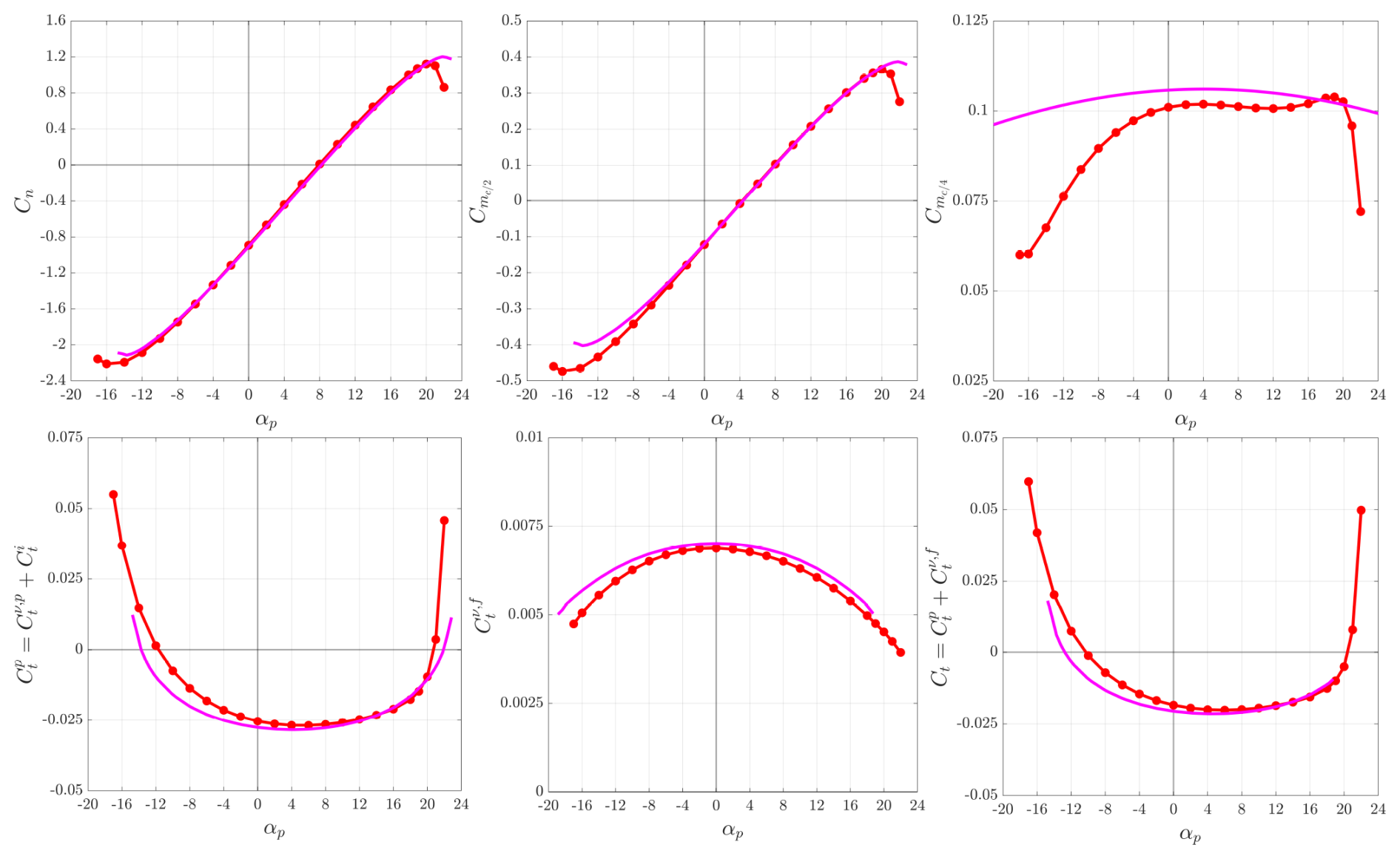
Figure 6 NACA0015 airfoil in rotation with $c/R=\mathrm{2}/\mathrm{7}$ and attached at $x_{\mathrm{p}}=c/\mathrm{4}$: comparison between the predicted values (magenta) of C_n, $C_{m_{c/\mathrm{2}}}$, $C_{m_{c/\mathrm{4}}}$, $C_{\mathrm{t}}^{\mathrm{p}}$, $C_{\mathrm{t}}^{\mathit{\nu },\mathrm{f}}$, C_t and the reference values obtained in CFD of the rotating airfoil (red).

3.5 Flat plate or thin airfoil attached at an arbitrary position

The case in which the attachment point is arbitrarily chosen can also be modeled. We then write

$$\begin{array}{}\text{(37)}& x_{\mathrm{p}}=(\mathrm{1}+\mathit{\delta }){\displaystyle \frac{c}{\mathrm{4}}},\end{array}$$

where δ is a chosen parameter. The canonic cases $x_{\mathrm{p}}=c/\mathrm{2}$ and $x_{\mathrm{p}}=c/\mathrm{4}$ investigated and modeled so far correspond, respectively, to δ=1 and δ=0.

The opening angle, α_v, between the attachment point x_p and the airfoil center $c/\mathrm{2}$ is obtained as

$$\begin{array}{}\text{(38)}& {\mathit{\alpha }}_v=\left({\displaystyle \frac{\mathrm{1}}{\mathrm{2}}}-{\displaystyle \frac{x_{\mathrm{p}}}{c}}\right){\displaystyle \frac{c}{R}}=(\mathrm{1}-\mathit{\delta }){\displaystyle \frac{c}{\mathrm{4}R}}=(\mathrm{1}-\mathit{\delta }){\mathit{\alpha }}_{\mathrm{c}}.\end{array}$$

We first consider the case of a flat plate without pitch angle (α_p=0). The horizontal plate is transformed into a tilted and cambered plate in the Z plane: its attachment point z_p=0 is transformed into Z_p=0, its center $z_{\mathrm{c}}=(\mathrm{1}-\mathit{\delta })c/\mathrm{4}$ is transformed into $(\mathrm{1}-\mathit{\delta })c/\mathrm{4}+\mathrm{i}(\mathrm{1}-\mathit{\delta }{)}^{\mathrm{2}}{c}^{\mathrm{2}}/(\mathrm{32}R)$, its trailing edge $z_{\mathrm{T}}=(\mathrm{3}-\mathit{\delta })c/\mathrm{4}$ is transformed into $Z_{\mathrm{T}}=(\mathrm{3}-\mathit{\delta })c/\mathrm{4}+\mathrm{i}(\mathrm{3}-\mathit{\delta }{)}^{\mathrm{2}}{c}^{\mathrm{2}}/(\mathrm{32}R)$ and its leading edge $z_{\mathrm{L}}=-(\mathrm{1}+\mathit{\delta })c/\mathrm{4}$ is transformed into $Z_{\mathrm{L}}=-(\mathrm{1}+\mathit{\delta })c/\mathrm{4}+\mathrm{i}(\mathrm{1}+\mathit{\delta }{)}^{\mathrm{2}}{c}^{\mathrm{2}}/(\mathrm{32}R)$. The slope of the tilted cambered plate at its center is then obtained as

$$\begin{array}{}\text{(39)}& {\left({\displaystyle \frac{\mathrm{d}Y}{\mathrm{d}X}}\right)}_{z_{\mathrm{c}}}=(\mathrm{1}-\mathit{\delta }){\displaystyle \frac{c}{\mathrm{4}R}}=(\mathrm{1}-\mathit{\delta }){\mathit{\alpha }}_{\mathrm{c}}={\mathit{\alpha }}_v.\end{array}$$

The angle of the cambered plate relative to the uniform horizontal velocity U is therefore also equal to α_v.

When further pitching the flat plate by an angle α_p, the angle α that the curved flow velocity vector at $c/\mathrm{4}$ makes relative to the plate is now

$$\begin{array}{}\text{(40)}& \mathit{\alpha }={\mathit{\alpha }}_{\mathrm{p}}+({\mathit{\alpha }}_{\mathrm{c}}-{\mathit{\alpha }}_v)={\mathit{\alpha }}_{\mathrm{p}}+\mathit{\delta }{\mathit{\alpha }}_{\mathrm{c}}.\end{array}$$

We also obtain

$$\begin{array}{}\text{(41)}& {\mathit{\alpha }}_{\mathrm{p}}-{\mathit{\alpha }}_v=\mathit{\alpha }-{\mathit{\alpha }}_{\mathrm{c}}.\end{array}$$

Using the same procedure as used for the cases with $x_{\mathrm{p}}=c/\mathrm{2}$ and $x_{\mathrm{p}}=c/\mathrm{4}$, we obtain the general models: for the flat plate and for thin airfoils without camber. We write them here for the airfoils. For the normal force coefficient C_n at the attachment point, we obtain

$$\begin{array}{}\text{(42)}& C_{\mathrm{n}}\left({\mathit{\alpha }}_{\mathrm{p}}\right)\simeq C_{\mathrm{l}}^{\mathrm{u}}({\mathit{\alpha }}_{\mathrm{p}}-{\mathit{\alpha }}_v)-C_{\mathrm{l}}^{\mathrm{u}}\left({\mathit{\alpha }}_{\mathrm{c}}\right).\end{array}$$

The moment coefficient at the plate center is again obtained from the potential flow theory as

$$\begin{array}{}\text{(43)}& C_{m_{c/\mathrm{2}}}\left({\mathit{\alpha }}_{\mathrm{p}}\right)\simeq C_{m_{c/\mathrm{2}}}^{\mathrm{0}}+{\displaystyle \frac{\mathrm{1}}{\mathrm{4}}}{C}_{\mathrm{l}}^{\mathrm{u}}({\mathit{\alpha }}_{\mathrm{p}}-{\mathit{\alpha }}_v)\cos ({\mathit{\alpha }}_{\mathrm{p}}-{\mathit{\alpha }}_v).\end{array}$$

This moment is indeed zero, as it should, for a plate (that has no $C_{m_{c/\mathrm{2}}}^{\mathrm{0}}$) when α_p=α_v as the cambered plate of the transformed flow is then horizontal.

The aerodynamic moment coefficients, $C_{m_{c/\mathrm{4}}}$ and $C_{m_{\text{ac}}}$, are then obtained as

$$\begin{array}{}\text{(44)}& \begin{array}{rl}{\displaystyle }{C}_{m_{c/\mathrm{4}}}\left({\mathit{\alpha }}_{\mathrm{p}}\right)=& {\displaystyle }{C}_{m_{c/\mathrm{2}}}\left({\mathit{\alpha }}_{\mathrm{p}}\right)-{\displaystyle \frac{\mathrm{1}}{\mathrm{4}}}{C}_{\mathrm{n}}\left({\mathit{\alpha }}_{\mathrm{p}}\right)\cos ({\mathit{\alpha }}_{\mathrm{p}}-{\mathit{\alpha }}_v)\\ {\displaystyle }\simeq & {\displaystyle }{C}_{m_{c/\mathrm{2}}}^{\mathrm{0}}+{\displaystyle \frac{\mathrm{1}}{\mathrm{4}}}{C}_{\mathrm{l}}^{\mathrm{u}}\left({\mathit{\alpha }}_{\mathrm{c}}\right)\cos ({\mathit{\alpha }}_{\mathrm{p}}-{\mathit{\alpha }}_v)\end{array}\end{array}$$

and

$$\begin{array}{}\text{(45)}& \begin{array}{rl}{\displaystyle }& {\displaystyle }{C}_{m_{\text{ac}}}\left({\mathit{\alpha }}_{\mathrm{p}}\right)=\\ {\displaystyle }& {\displaystyle }{C}_{m_{c/\mathrm{2}}}\left({\mathit{\alpha }}_{\mathrm{p}}\right)-\left({\displaystyle \frac{\mathrm{1}}{\mathrm{2}}}-{\displaystyle \frac{x_{\text{ac}}}{c}}\right)C_{\mathrm{n}}\left({\mathit{\alpha }}_{\mathrm{p}}\right)\cos ({\mathit{\alpha }}_{\mathrm{p}}-{\mathit{\alpha }}_v).\end{array}\end{array}$$

In the same way, the model for the moment coefficient around the attachment point is obtained as

$$\begin{array}{}\text{(46)}& \begin{array}{rl}{\displaystyle }& {\displaystyle }{C}_{m_{x_{\mathrm{p}}}}\left({\mathit{\alpha }}_{\mathrm{p}}\right)\simeq \\ {\displaystyle }& {\displaystyle }{C}_{m_{c/\mathrm{2}}}\left({\mathit{\alpha }}_{\mathrm{p}}\right)-\left({\displaystyle \frac{\mathrm{1}}{\mathrm{2}}}-{\displaystyle \frac{x_{\mathrm{p}}}{c}}\right)C_{\mathrm{n}}\left({\mathit{\alpha }}_{\mathrm{p}}\right)\cos ({\mathit{\alpha }}_{\mathrm{p}}-{\mathit{\alpha }}_v).\end{array}\end{array}$$

As the moment $m_{\mathrm{0}}=m_{x_{\mathrm{p}}}+R{f}_{\mathrm{t}}^{\mathrm{i}}$ around the center of rotation of the arm must still be zero in inviscid flow, the model for the tangential force coefficient in inviscid flow becomes

$$\begin{array}{}\text{(47)}& C_{\mathrm{t}}^{\mathrm{i}}\left({\mathit{\alpha }}_{\mathrm{p}}\right)\simeq -{\displaystyle \frac{c}{R}}{C}_{m_{x_{\mathrm{p}}}}\left({\mathit{\alpha }}_{\mathrm{p}}\right),\end{array}$$

and hence the model for viscous flow is now taken as

$$\begin{array}{}\text{(48)}& \begin{array}{rl}{\displaystyle }{C}_{\mathrm{t}}\left({\mathit{\alpha }}_{\mathrm{p}}\right)=& {\displaystyle }{C}_{\mathrm{t}}^{\mathit{\nu }}\left({\mathit{\alpha }}_{\mathrm{p}}\right)+C_{\mathrm{t}}^{\mathrm{i}}\left({\mathit{\alpha }}_{\mathrm{p}}\right)\\ {\displaystyle }=& {\displaystyle }\left(C_{\mathrm{t}}^{\mathit{\nu },\mathrm{p}}\left({\mathit{\alpha }}_{\mathrm{p}}\right)+C_{\mathrm{t}}^{\mathrm{i}}\left({\mathit{\alpha }}_{\mathrm{p}}\right)\right)+C_{\mathrm{t}}^{\mathit{\nu },\mathrm{f}}\left({\mathit{\alpha }}_{\mathrm{p}}\right)\\ {\displaystyle }& {\displaystyle }=C_{\mathrm{t}}^{\mathrm{p}}\left({\mathit{\alpha }}_{\mathrm{p}}\right)+C_{\mathrm{t}}^{\mathit{\nu },\mathrm{f}}\left({\mathit{\alpha }}_{\mathrm{p}}\right)\\ {\displaystyle }\simeq & {\displaystyle }\left(C_{\mathrm{d}}^{\text{u,p}}({\mathit{\alpha }}_{\mathrm{p}}-{\mathit{\alpha }}_v)-{\displaystyle \frac{c}{R}}{C}_{m_{x_{\mathrm{p}}}}\left({\mathit{\alpha }}_{\mathrm{p}}\right)\right)\\ {\displaystyle }& {\displaystyle }+C_{\mathrm{d}}^{\text{u,f}}\left(\right({\mathit{\alpha }}_{\mathrm{p}}-{\mathit{\alpha }}_v)+{\mathit{\alpha }}_{\mathrm{c}}).\end{array}\end{array}$$

Again, if the moment $m_{x_{\mathrm{p}}}$ is not enforced in the ALM, then only $f_{\mathrm{t}}^{\mathit{\nu }}$ must be enforced, while $f_{\mathrm{t}}^{\mathrm{i}}$ must be ignored.

Finally, the force coefficients can also be decomposed into the usual aerodynamic coefficients considered at $c/\mathrm{4}$ by using the angle of attack α_p+δ α_c that the curved flow velocity vector makes there relative to the airfoil chord:

$$\begin{array}{}\text{(49)}& \begin{array}{rl}{\displaystyle }{C}_{\mathrm{l}}=& {\displaystyle }{C}_{\mathrm{n}}\left({\mathit{\alpha }}_{\mathrm{p}}\right)\cos \left(\mathit{\delta }{\mathit{\alpha }}_{\mathrm{c}}\right)-C_{\mathrm{t}}\left({\mathit{\alpha }}_{\mathrm{p}}\right)\sin \left(\mathit{\delta }{\mathit{\alpha }}_{\mathrm{c}}\right),\\ {\displaystyle }{C}_{\mathrm{d}}=& {\displaystyle }{C}_{\mathrm{n}}\left({\mathit{\alpha }}_{\mathrm{p}}\right)\sin \left(\mathit{\delta }{\mathit{\alpha }}_{\mathrm{c}}\right)+C_{\mathrm{t}}\left({\mathit{\alpha }}_{\mathrm{p}}\right)\cos \left(\mathit{\delta }{\mathit{\alpha }}_{\mathrm{c}}\right).\end{array}\end{array}$$

4 Actuator line method for imposing the aerodynamic forces

We briefly recall the actuator line method (ALM) which is used here to model the effect of the airfoil forces on the flow. It was detailed in Trigaux et al. (2024b) as implemented in a fourth-order incompressible flow solver using finite differences. It was also used in Trigaux et al. (2024a) for aero-elastic studies of a 15 MW horizontal-axis turbine.

At each time step, the vector force per unit span −f that the airfoil exerts on the flow (i.e., the opposite of the vector force f that the flow exerts on the airfoil) is distributed over the neighboring grid points of the flow solver. In all that follows, the term “force” is understood as “force per unit span”. This is achieved using a 2-D Gaussian kernel centered at the airfoil AC location and whose (x,y) frame is fixed relative to the airfoil.

The force field applied to the flow solver is as follows:

$$\begin{array}{}\text{(50)}& {\mathit{f}}^{\mathrm{s}}(x,y)=-{\mathit{\eta }}_{\text{2D}}(x,y)\mathit{f}\text{where}\mathit{f}=f_x{\widehat{\mathit{e}}}_x+f_y{\widehat{\mathit{e}}}_y\end{array}$$

and

$$\begin{array}{}\text{(51)}& \begin{array}{rl}{\displaystyle }{\mathit{\eta }}_{\text{2D}}(x,y)=& {\displaystyle }{\mathit{\eta }}_{{\mathit{\sigma }}_{\mathrm{c}}}\left(x\right){\mathit{\eta }}_{{\mathit{\sigma }}_{\mathrm{t}}}\left(y\right)\\ {\displaystyle }=& {\displaystyle \frac{\mathrm{1}}{\sqrt{\mathit{\pi }}{\mathit{\sigma }}_{\mathrm{c}}}}\exp \left(-{\displaystyle \frac{x^{\mathrm{2}}}{{\mathit{\sigma }}_{\mathrm{c}}^{\mathrm{2}}}}\right){\displaystyle \frac{\mathrm{1}}{\sqrt{\mathit{\pi }}{\mathit{\sigma }}_{\mathrm{t}}}}\exp \left(-{\displaystyle \frac{y^{\mathrm{2}}}{{\mathit{\sigma }}_{\mathrm{t}}^{\mathrm{2}}}}\right),\end{array}\end{array}$$

with σ_c the core size in the airfoil chord direction and σ_t that in the thickness direction. Here, we use an isotropic kernel (${\mathit{\sigma }}_{\mathrm{c}}={\mathit{\sigma }}_{\mathrm{t}}=\mathit{\sigma }$) and with $\mathit{\sigma }=c/\mathrm{4}$ as recommended by Martínez-Tossas et al. (2017). The kernel is discretized using a 2-D template that consists of $(\mathrm{2}n+\mathrm{1})(\mathrm{2}n+\mathrm{1})$ cells of size h×h. A node is located at the center of each cell $(x_i,y_j)=(ih,jh)$, and the kernel is integrated analytically over that cell to obtain the weight. For the integration in x, we obtain, for $\mathrm{0}\le i<n$,

$$\begin{array}{}\text{(52)}& \begin{array}{rl}{\displaystyle }{w}_i=& {\displaystyle }{\int }_{x_i-h/\mathrm{2}}^{x_i+h/\mathrm{2}}{\mathit{\eta }}_{\mathit{\sigma }}\left(x\right)\mathrm{d}x\\ {\displaystyle }=& {\displaystyle \frac{\mathrm{1}}{\mathrm{2}}}\left[\text{erf}\left({\displaystyle \frac{x_i+h/\mathrm{2}}{\mathit{\sigma }}}\right)-\text{erf}\left({\displaystyle \frac{x_i-h/\mathrm{2}}{\mathit{\sigma }}}\right)\right].\end{array}\end{array}$$

For the cell i=n, we include the part outside (to ensure that the sum of the weights is unity):

$$\begin{array}{}\text{(53)}& w_n=\underset{x_n-h/\mathrm{2}}{\overset{\mathrm{\infty }}{\int }}{\mathit{\eta }}_{\mathit{\sigma }}\left(x\right)\mathrm{d}x={\displaystyle \frac{\mathrm{1}}{\mathrm{2}}}\left[\mathrm{1}-\text{erf}\left({\displaystyle \frac{x_n-h/\mathrm{2}}{\mathit{\sigma }}}\right)\right].\end{array}$$

By symmetry, we have $w_{-i}=w_i$. The weights in y are w_j=w_i for j=i. The weight associated with the (i,j) cell is then $w_{i,j}=w_i{w}_j$ and the associated force is

$$\begin{array}{}\text{(54)}& {\mathit{f}}_{i,j}^{\mathrm{s}}=-w_i{w}_j\mathit{f}.\end{array}$$

We use $h=\mathit{\sigma }/\mathrm{2}$ and n=4. The weights w_i are provided in Table 1. As the kernel was integrated over each cell of the template, we ensure that the forces are completely imposed to the flow solver.

Table 1 Weights w_i associated with the 1-D Gaussian kernel for the case with $h=\mathit{\sigma }/\mathrm{2}$ and using n=4. The numbers provided have been rounded so that ${\sum }_{i=-\mathrm{4}}^{\mathrm{4}}{w}_i=\mathrm{1}$ exactly.

In the present implementation of the ALM used for modeling a VAT configuration, an overset mesh technique is employed, in which the flow solver mesh covering the turbine region, including the AL and its template, rotates together with the blade; see Fig. 9. Note that, when the AL and its template move through the flow solver grid, as in Trigaux et al. (2024a), the fraction ${\mathit{f}}_{i,j}^{\mathrm{s}}$ of the force on each cell of the template must be further distributed to the nearest flow solver grid points. This is done using a bi-linear distribution kernel, ensuring that each fraction is distributed to the nearest grid points.

The effective velocity vector to be used in the ALM is obtained by using a weighted average of the velocity vectors provided by the flow solver around the control point (equal to the center of the Gaussian kernel, typically taken as the location of the aerodynamic center), their relative weighting being determined using the same template as that used for the force distribution. This procedure corresponds to “integral sampling” (as opposed to “pointwise sampling”) and has been shown to provide slightly better results (Merabet and Laurendeau, 2019; Caprace et al., 2020). The effective velocity vector at the control point, v, is thus measured using

$$\begin{array}{}\text{(55)}& \mathit{v}=\sum _{i=-n_x}^{n_x}\sum _{j=-n_y}^{n_y}{w}_i{w}_j\mathit{v}(x_i,y_j).\end{array}$$

When the airfoil is moving relative to the fixed reference frame, as is the case in the present work, we must add this relative velocity to the flow solver velocity field since the ALM requires the apparent velocity seen by the airfoil, V.

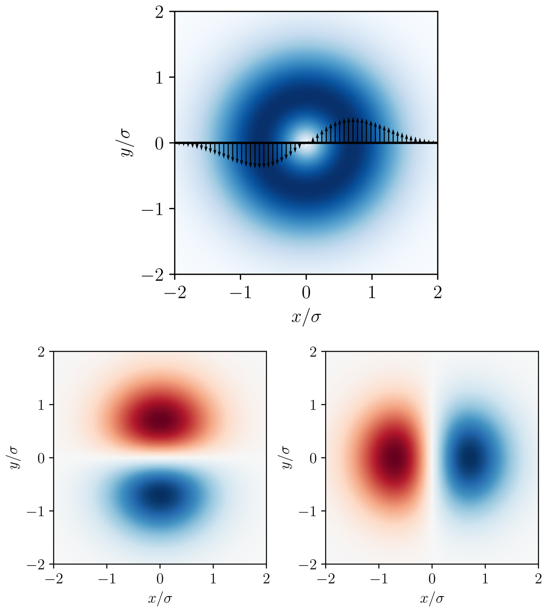
Figure 7 Vector field ${\mathit{g}}^{\mathrm{s}}(x,y)/m_{\text{ac}}=g\left(r\right){\widehat{\mathit{e}}}_{\mathit{\theta }}$ used for the moment distribution (top) and its components (bottom): $g_x^{\mathrm{s}}(x,y)/m_{\text{ac}}$ along ${\widehat{\mathit{e}}}_x$ (left) and $g_y^{\mathrm{s}}(x,y)/m_{\text{ac}}$ along ${\widehat{\mathit{e}}}_y$ (right).

Moreover, when the parasitic drag is significant, the apparent velocity vector, V, is not yet the suitable vector to use in the ALM, as it also contains the spurious velocity component induced by the wake vorticity associated with the parasitic drag. This induced velocity can be estimated using the procedure described in Martínez-Tossas et al. (2017). Assuming that the wake is shed primarily in the direction of V, the corrected apparent velocity is

$$\begin{array}{}\text{(56)}& {\mathit{V}}^{\text{corr}}={\displaystyle \frac{\mathit{V}}{\left(\mathrm{1}-\frac{\mathrm{1}}{\mathrm{4}\sqrt{\mathit{\pi }}}\frac{c}{\mathit{\sigma }}{C}_{\mathrm{d}}^{\mathit{\nu }}\right)}}.\end{array}$$

As $C_{\mathrm{d}}^{\mathit{\nu }}$ is used in the above correction, a few iterations are required to determine all values; alternatively, the value of the previous time step can be used.

Once we have V^corr, we measure the angle that this vector makes relative to the airfoil chord. Using this angle and the norm V^corr of the velocity, we can compute, using the airfoil polar model, the lift and drag forces exerted by the flow on the airfoil.

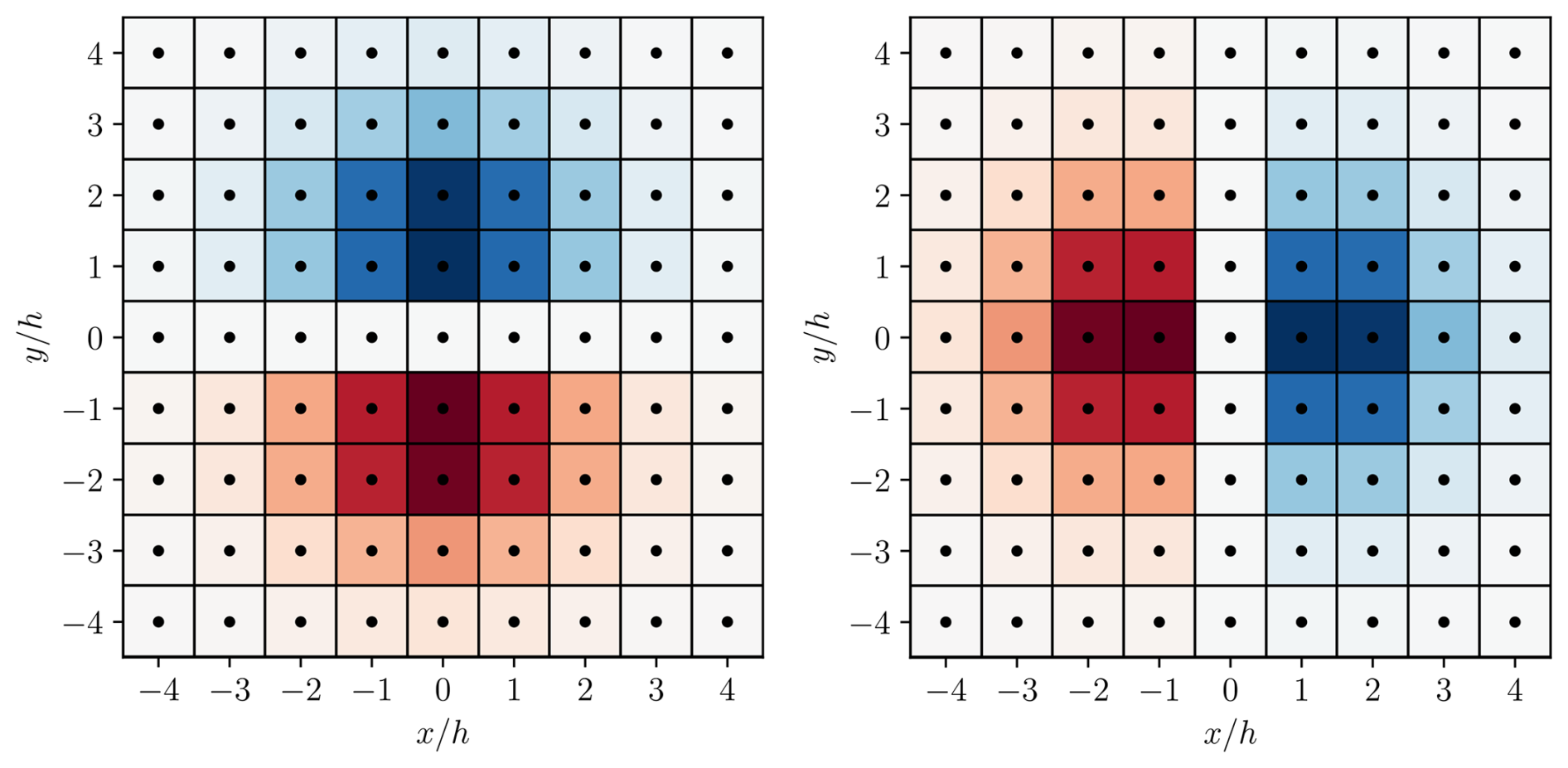
Figure 8 Template used for the moment distribution for the case with $h=\mathit{\sigma }/\mathrm{2}$ and using n=4. The color intensity of each (i,j) cell is proportional to its weights: w_i q_j (left) and q_i w_j (right).

5 Actuator line method for imposing an aerodynamic moment

The previous section was devoted to presenting our particular implementation of the ALM aimed at efficiently distributing the aerodynamic force acting on the airfoil onto the nearby flow solver grid points, using a 2D template corresponding to the discretization of a Gaussian kernel. The same template is also used to evaluate the effective velocity required to compute the aerodynamic forces.

Table 2 Weights q_j for the case with $h=\mathit{\sigma }/\mathrm{2}$ and using n=4. By anti-symmetry, $q_{-j}=-q_j$.

As such, however, the ALM cannot handle any aerodynamic moment. We extend the actuator line method to enable the distribution of an aerodynamic moment. Of course, a pure aerodynamic moment cannot be imposed, as the ALM uses a distribution kernel of some size σ. We hence replace the aerodynamic moment by a force field that has the same net effect, as presented in Fig. 7; we then discretize this force field using the 2D template.

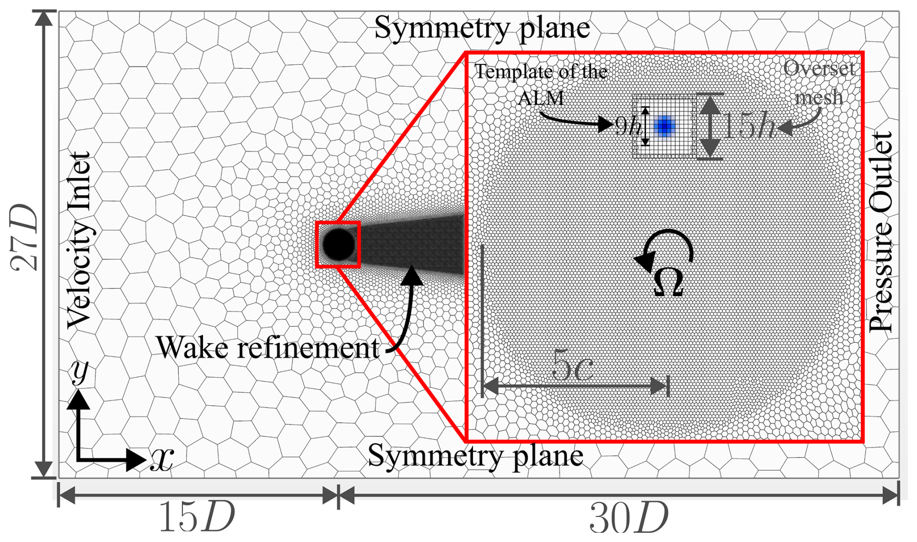
Figure 9 Computational domain and mesh used for the ALM simulations. The turbine region, including the template of the ALM, is implemented using an overset mesh approach to enable the 2-D template as described in Sects. 4 and 5. The weights for the application of the forces are also illustrated in blue.

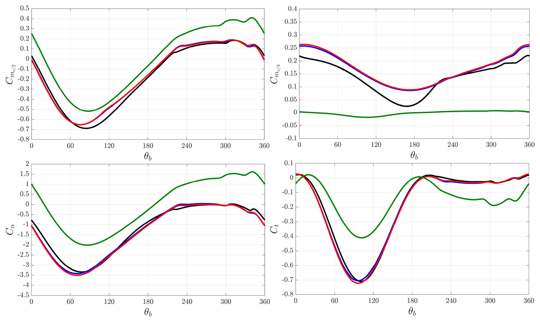
Figure 10 VAT with NACA0015 airfoil attached at $x_{\mathrm{p}}=c/\mathrm{4}$ and operating at TSR=3.25: comparison between the ALM with $m_{c/\mathrm{4}}$ and $f_{\mathrm{t}}^{\mathrm{i}}$ explicitly enforced (red), the ALM without $m_{c/\mathrm{4}}$ and $f_{\mathrm{t}}^{\mathrm{i}}$ explicitly enforced (blue) and the wall-resolved reference simulation (black) of $C_{m_{c/\mathrm{2}}}$, $C_{m_{c/\mathrm{4}}}$, C_n and C_t. The results of the ALM without curvature corrections are also shown for comparison (green).

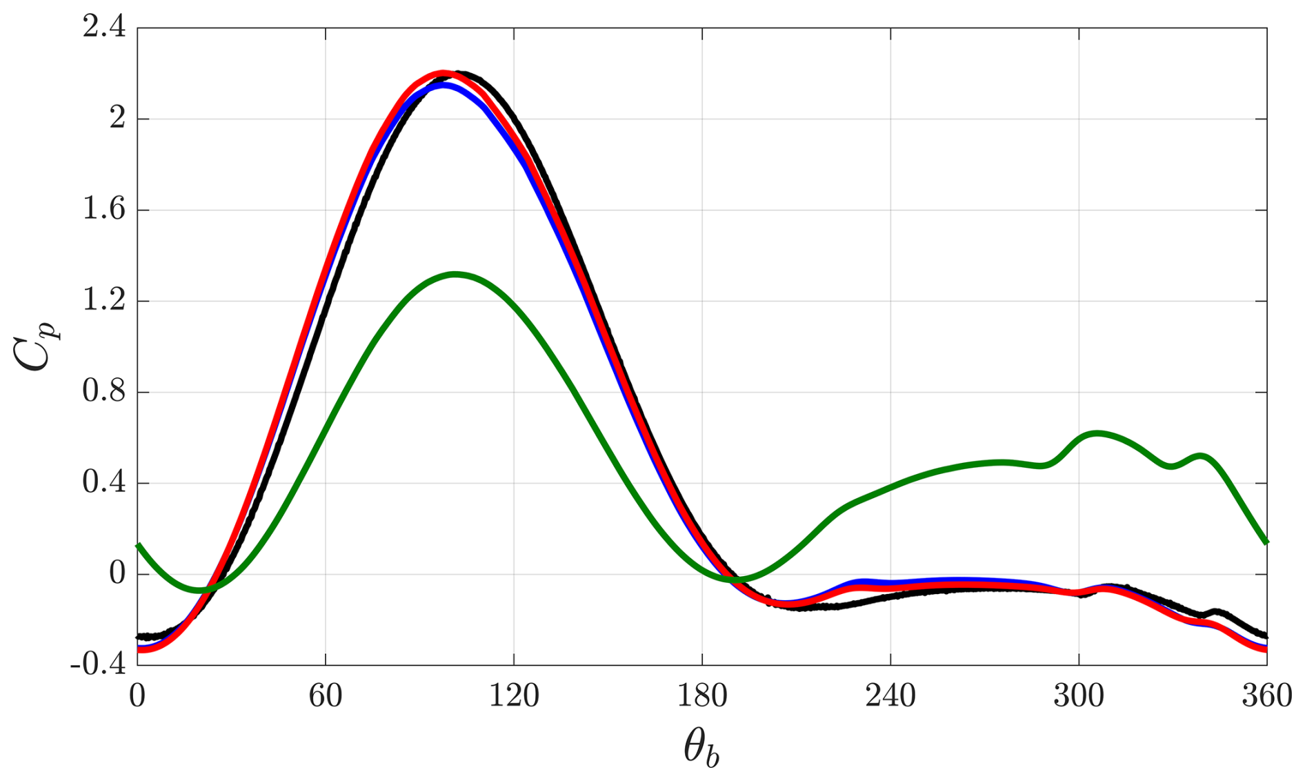
Figure 11 VAT with NACA0015 airfoil attached at $x_{\mathrm{p}}=c/\mathrm{4}$ and operating at TSR=3.25: comparison between the results of the ALM with $m_{c/\mathrm{4}}$ and $f_{\mathrm{t}}^{\mathrm{i}}$ explicitly enforced (red), the ALM without $m_{c/\mathrm{4}}$ and $f_{\mathrm{t}}^{\mathrm{i}}$ explicitly enforced (blue) and the wall-resolved reference simulation (black) of C_p. The results of the ALM without curvature corrections are also shown for comparison (green).

Assume that the flow exerts a pitching moment per unit span m_ac around the airfoil aerodynamic center. Recall that the pitching moment is, by convention, positive when it acts to pitch the airfoil in the nose-up direction. The airfoil hence exerts a moment −m_ac on the flow. This effect can be achieved by imposing the following annular force field:

$$\begin{array}{}\text{(57)}& {\mathit{g}}^{\mathrm{s}}(x,y)=g\left(r\right){\widehat{\mathit{e}}}_{\mathit{\theta }}{m}_{\text{ac}}\end{array}$$

with

$$\begin{array}{}\text{(58)}& \begin{array}{rl}{\displaystyle }g\left(r\right)=& {\displaystyle }-{\displaystyle \frac{\mathrm{1}}{\mathrm{2}\mathit{\pi }{\mathit{\sigma }}^{\mathrm{2}}}}{\displaystyle \frac{\mathrm{d}}{\mathrm{d}r}}\left(\exp \left(-{\displaystyle \frac{r^{\mathrm{2}}}{{\mathit{\sigma }}^{\mathrm{2}}}}\right)\right)\\ {\displaystyle }=& {\displaystyle \frac{\mathrm{1}}{\mathit{\pi }{\mathit{\sigma }}^{\mathrm{3}}}}{\displaystyle \frac{r}{\mathit{\sigma }}}\exp \left(-{\displaystyle \frac{r^{\mathrm{2}}}{{\mathit{\sigma }}^{\mathrm{2}}}}\right),\end{array}\end{array}$$

which indeed satisfies $\iint rg\left(r\right)\mathrm{d}S=\mathrm{1}$ where dS=r dθ dr:

$$\begin{array}{}\text{(59)}& \begin{array}{rl}{\displaystyle }\iint rg\left(r\right)\mathrm{d}S=& {\displaystyle }\mathrm{2}\mathit{\pi }{\int }_{\mathrm{0}}^{\mathrm{\infty }}g\left(r\right)r^{\mathrm{2}}\mathrm{d}r\\ {\displaystyle }=& {\displaystyle }\mathrm{2}{\int }_{\mathrm{0}}^{\mathrm{\infty }}\exp \left(-{\displaystyle \frac{r^{\mathrm{2}}}{{\mathit{\sigma }}^{\mathrm{2}}}}\right){\displaystyle \frac{r^{\mathrm{3}}}{{\mathit{\sigma }}^{\mathrm{3}}}}{\displaystyle \frac{\mathrm{d}r}{\mathit{\sigma }}}\\ {\displaystyle }=& {\displaystyle }\mathrm{2}{\int }_{\mathrm{0}}^{\mathrm{\infty }}\exp \left(-s^{\mathrm{2}}\right)s^{\mathrm{3}}\mathrm{d}s\\ {\displaystyle }=& {\displaystyle }{\int }_{\mathrm{0}}^{\mathrm{\infty }}\exp (-p)p\mathrm{d}p=\mathrm{1},\end{array}\end{array}$$

where we have used the changes in variable $s=r/\mathit{\sigma }$ and p=s² and where the last integral has been evaluated by parts.

This force field corresponds to applying a net moment of −m_ac to the flow, without applying any net force. The applied force field per unit m_ac is illustrated at the top of Fig. 7; it is indeed counter-clockwise when m_ac is positive. It can be decomposed as

$$\begin{array}{}\text{(60)}& \begin{array}{rl}{\displaystyle }& {\displaystyle }{\mathit{g}}^{\mathrm{s}}(x,y)\\ {\displaystyle }& {\displaystyle }=g\left(r\right){\widehat{\mathit{e}}}_{\mathit{\theta }}{m}_{\text{ac}}=g\left(r\right)\left(-\sin \mathit{\theta }{\widehat{\mathit{e}}}_x+\cos \mathit{\theta }{\widehat{\mathit{e}}}_y\right)m_{\text{ac}}\\ {\displaystyle }& {\displaystyle }={\displaystyle \frac{\mathrm{1}}{\mathit{\pi }{\mathit{\sigma }}^{\mathrm{3}}}}{\displaystyle \frac{r}{\mathit{\sigma }}}\exp \left(-{\displaystyle \frac{r^{\mathrm{2}}}{{\mathit{\sigma }}^{\mathrm{2}}}}\right)\left(-\sin \mathit{\theta }{\widehat{\mathit{e}}}_x+\cos \mathit{\theta }{\widehat{\mathit{e}}}_y\right)m_{\text{ac}}.\end{array}\end{array}$$

Since x=rcos θ and y=rsin θ, we finally obtain ${\mathit{g}}^{\mathrm{s}}(x,y)=g_x^{\mathrm{s}}(x,y){\widehat{\mathit{e}}}_x+g_y^{\mathrm{s}}(x,y){\widehat{\mathit{e}}}_y$ with

$$\begin{array}{}\text{(61)}& \begin{array}{rl}{\displaystyle }{g}_x^{\mathrm{s}}(x,y)=& {\displaystyle }-{\displaystyle \frac{\mathrm{1}}{\mathit{\pi }{\mathit{\sigma }}^{\mathrm{3}}}}{\displaystyle \frac{y}{\mathit{\sigma }}}\exp \left(-{\displaystyle \frac{x^{\mathrm{2}}+y^{\mathrm{2}}}{{\mathit{\sigma }}^{\mathrm{2}}}}\right)m_{\text{ac}}\\ {\displaystyle }=& {\displaystyle }-{\mathit{\eta }}_{\mathit{\sigma }}\left(x\right)\left({\displaystyle \frac{y}{\mathit{\sigma }}}{\mathit{\eta }}_{\mathit{\sigma }}\left(y\right)\right){\displaystyle \frac{m_{\text{ac}}}{\mathit{\sigma }}},\\ {\displaystyle }{g}_y^{\mathrm{s}}(x,y)=& {\displaystyle \frac{\mathrm{1}}{\mathit{\pi }{\mathit{\sigma }}^{\mathrm{3}}}}{\displaystyle \frac{x}{\mathit{\sigma }}}\exp \left(-{\displaystyle \frac{x^{\mathrm{2}}+y^{\mathrm{2}}}{{\mathit{\sigma }}^{\mathrm{2}}}}\right)m_{\text{ac}}\\ {\displaystyle }=& {\displaystyle }\left({\displaystyle \frac{x}{\mathit{\sigma }}}{\mathit{\eta }}_{\mathit{\sigma }}\left(x\right)\right){\mathit{\eta }}_{\mathit{\sigma }}\left(y\right){\displaystyle \frac{m_{\text{ac}}}{\mathit{\sigma }}}.\end{array}\end{array}$$

These components are illustrated at the bottom of Fig. 7.

Table 3 Mean $C_{m_{c/\mathrm{2}}}$, $C_{m_{c/\mathrm{4}}}$, C_n, C_t and C_p over a blade cycle for a VAT with airfoil attached at $x_{\mathrm{p}}=c/\mathrm{4}$ and operating at TSR=3.25. The results of the ALM without curvature corrections are also reported for comparison.

The above equations are then integrated analytically over each cell of the 2D template to obtain the values of the weights. We obtain

$$\begin{array}{}\text{(62)}& \begin{array}{rl}{\displaystyle }& {\displaystyle }{\int }_{x_i-h/\mathrm{2}}^{x_i+h/\mathrm{2}}{\int }_{y_j-h/\mathrm{2}}^{y_j+h/\mathrm{2}}{g}_x^{\mathrm{s}}(x,y)\mathrm{d}x\mathrm{d}y=\\ {\displaystyle }& {\displaystyle }-\left({\int }_{x_i-h/\mathrm{2}}^{x_i+h/\mathrm{2}}{\mathit{\eta }}_{\mathit{\sigma }}\left(x\right)\mathrm{d}x\right)\left({\int }_{y_j-h/\mathrm{2}}^{y_j+h/\mathrm{2}}{\displaystyle \frac{y}{\mathit{\sigma }}}{\mathit{\eta }}_{\mathit{\sigma }}\left(y\right)\mathrm{d}y\right){\displaystyle \frac{m_{\text{ac}}}{\mathit{\sigma }}}.\end{array}\end{array}$$

The first integral has already been evaluated: it is w_i. Let us evaluate the second integral, which we denote q_j. For $\mathrm{0}\le j<n$, we obtain

$$\begin{array}{}\text{(63)}& \begin{array}{rl}{\displaystyle }{q}_j=& {\displaystyle }{\int }_{y_j-h/\mathrm{2}}^{y_j+h/\mathrm{2}}{\displaystyle \frac{y}{\mathit{\sigma }}}{\mathit{\eta }}_{\mathit{\sigma }}\left(y\right)\mathrm{d}y={\displaystyle \frac{\mathrm{1}}{\sqrt{\mathit{\pi }}}}{\int }_{y_j-h/\mathrm{2}}^{y_j+h/\mathrm{2}}{\displaystyle \frac{y}{\mathit{\sigma }}}\exp \left(-{\displaystyle \frac{y^{\mathrm{2}}}{{\mathit{\sigma }}^{\mathrm{2}}}}\right){\displaystyle \frac{\mathrm{d}y}{\mathit{\sigma }}}\\ {\displaystyle }=& {\displaystyle \frac{\mathrm{1}}{\sqrt{\mathit{\pi }}}}{\int }_{(y_j-h/\mathrm{2})/\mathit{\sigma }}^{(y_j+h/\mathrm{2})/\mathit{\sigma }}s\exp \left(-s^{\mathrm{2}}\right)\mathrm{d}s\\ {\displaystyle }=& {\displaystyle \frac{\mathrm{1}}{\mathrm{2}\sqrt{\mathit{\pi }}}}{\int }_{(y_j-h/\mathrm{2}{)}^{\mathrm{2}}/{\mathit{\sigma }}^{\mathrm{2}}}^{(y_j+h/\mathrm{2}{)}^{\mathrm{2}}/{\mathit{\sigma }}^{\mathrm{2}}}\exp (-p)\mathrm{d}p\\ {\displaystyle }=& {\displaystyle \frac{\mathrm{1}}{\mathrm{2}\sqrt{\mathit{\pi }}}}\left[\exp \left(-{\displaystyle \frac{(y_j-h/\mathrm{2}{)}^{\mathrm{2}}}{{\mathit{\sigma }}^{\mathrm{2}}}}\right)-\exp \left(-{\displaystyle \frac{(y_j+h/\mathrm{2}{)}^{\mathrm{2}}}{{\mathit{\sigma }}^{\mathrm{2}}}}\right)\right].\end{array}\end{array}$$

By anti-symmetry, we have $q_{-j}=-q_j$ and q₀=0. For the weight associated with the boundary cell j=n, the integration again includes the part of the kernel outside:

$$\begin{array}{}\text{(64)}& \begin{array}{rl}{\displaystyle }{q}_j=& {\displaystyle }{\int }_{y_n-h/\mathrm{2}}^{\mathrm{\infty }}{\displaystyle \frac{y}{\mathit{\sigma }}}{\mathit{\eta }}_{\mathit{\sigma }}\left(y\right)\mathrm{d}y\\ {\displaystyle }=& {\displaystyle \frac{\mathrm{1}}{\mathrm{2}\sqrt{\mathit{\pi }}}}\left[\exp \left(-{\displaystyle \frac{(y_j-h/\mathrm{2}{)}^{\mathrm{2}}}{{\mathit{\sigma }}^{\mathrm{2}}}}\right)\right].\end{array}\end{array}$$

We hence finally obtain, for the (i,j) cell,

$$\begin{array}{}\text{(65)}& \underset{x_i-h/\mathrm{2}}{\overset{x_i+h/\mathrm{2}}{\int }}\underset{y_j-h/\mathrm{2}}{\overset{y_j+h/\mathrm{2}}{\int }}{g}_x^{\mathrm{s}}(x,y)\mathrm{d}x\mathrm{d}y=-w_i{q}_j{\displaystyle \frac{m_{\text{ac}}}{\mathit{\sigma }}}.\end{array}$$

Following the same procedure, we also obtain

$$\begin{array}{}\text{(66)}& \underset{x_i-h/\mathrm{2}}{\overset{x_i+h/\mathrm{2}}{\int }}\underset{y_j-h/\mathrm{2}}{\overset{y_j+h/\mathrm{2}}{\int }}{g}_y^{\mathrm{s}}(x,y)\mathrm{d}x\mathrm{d}y=q_i{w}_j{\displaystyle \frac{m_{\text{ac}}}{\mathit{\sigma }}}.\end{array}$$

The weights w_i q_j and q_i w_j are illustrated in Fig. 8. We stress that our method imposes the net moment whatever the choice of σ. We hence can use the same value of σ as that used for imposing the forces, also for simplicity.

In summary, the ALM that imposes both the aerodynamic force f and moment m_ac amounts to distributing the following force on each (i,j) cell:

$$\begin{array}{}\text{(67)}& -\left(w_i{w}_j{f}_x+w_i{q}_j{\displaystyle \frac{m_{\text{ac}}}{\mathit{\sigma }}}\right){\widehat{\mathit{e}}}_x-\left(w_i{w}_j{f}_y-q_i{w}_j{\displaystyle \frac{m_{\text{ac}}}{\mathit{\sigma }}}\right){\widehat{\mathit{e}}}_y.\end{array}$$

As the two components of the kernel were integrated over each cell of the template, we ensure that the moment is completely imposed to the flow solver.

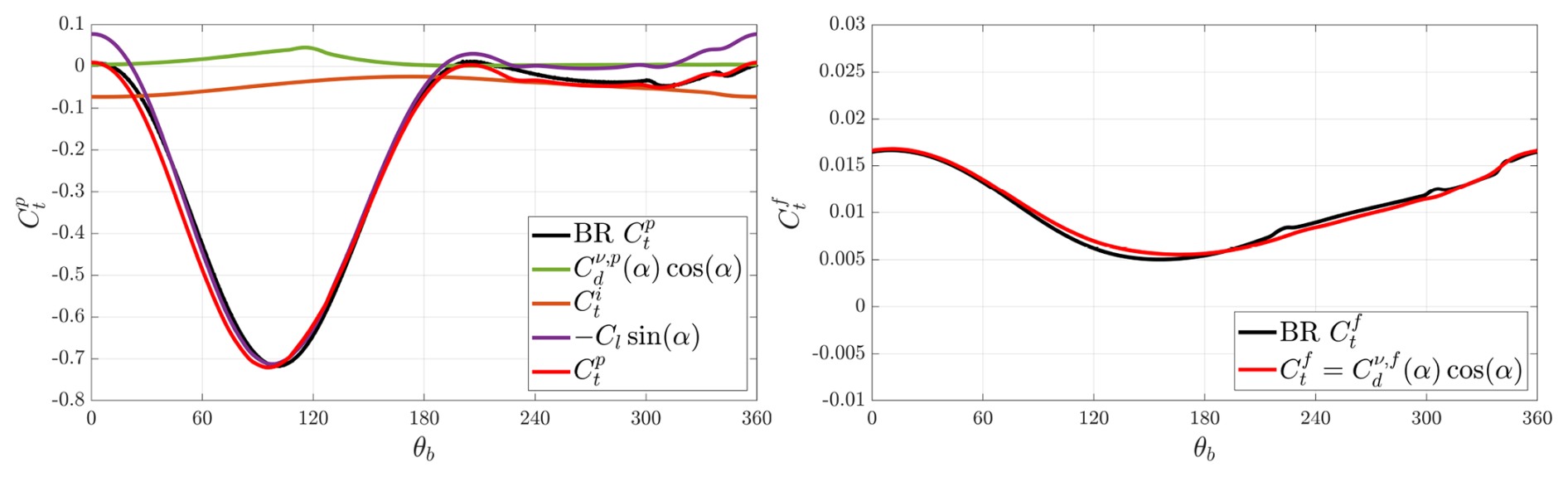
Figure 12 VAT with NACA0015 airfoil attached at $x_{\mathrm{p}}=c/\mathrm{4}$ and operating at TSR=3.25: comparison between the ALM with $m_{c/\mathrm{4}}$ and $f_{\mathrm{t}}^{\mathrm{i}}$ explicitly enforced (red) and the reference wall-resolved simulation (black) of the pressure contribution $C_{\mathrm{t}}^{\mathrm{p}}$ (with its components) and of the friction contribution $C_{\mathrm{t}}^f$ to the tangential force coefficient.

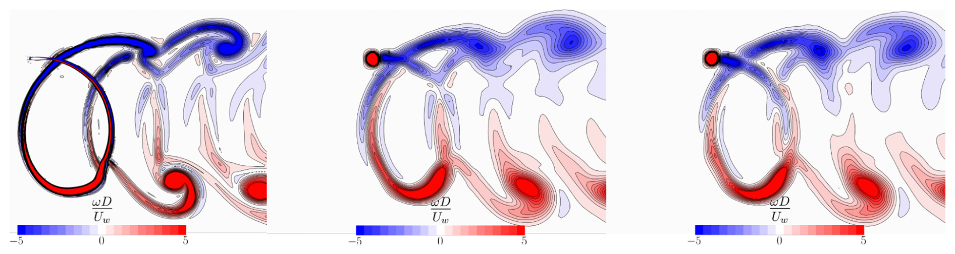
Figure 13 Vorticity field for the wall-resolved simulation (left), the ALM simulation without $m_{c/\mathrm{4}}$ enforced (center) and the ALM simulation with $m_{c/\mathrm{4}}$ enforced (right).

6 Results: corrected ALM applied to a VAT configuration and comparison with CFD data

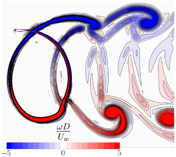
We consider the single-blade VAT configuration that was studied by Villeneuve et al. (2021). The blade profile is the NACA0015 airfoil considered previously. It is attached to the arm without pitch angle. The blade is rotating counterclockwise at the angular velocity Ω and the upstream flow, at velocity U_w, is coming from the left. The tip speed ratio is $\text{TSR}=\frac{\mathrm{\Omega }R}{U_w}$. The simulated case corresponds to TSR=3.25, which is the value at which the produced power is maximized. This value is also high enough that the flow past the blade does not separate dynamically at any position over the cycle; as is confirmed when examining the vorticity field of the wall-resolved simulation in Fig. 13. Hence, using the static airfoil polar data, solely corrected for flow curvature effects (i.e., no added dynamic polar model), is expected to be sufficient.

All simulations are conducted under the incompressible flow assumption. The ALM and wall-resolved simulations are performed using the finite-volume solver Siemens^® STAR-CCM+^®. The URANS equations are solved in conjunction with the Spalart–Allmaras turbulence closure model. A uniform velocity is imposed at the inlet, and a turbulent to molecular viscosity ratio of ${\mathit{\nu }}_{\mathrm{t}}/\mathit{\nu }=\mathrm{0.2}$ is used, representative of a clean flow. A uniform static pressure is imposed at the outlet. The far lateral boundaries are symmetry planes.

Second-order schemes are employed for the spatial discretization of both the convective and diffusive fluxes. The temporal integration is carried out using the second-order implicit unsteady scheme, and one turbine revolution is discretized into 1000 time steps. The pressure–velocity coupling is handled using the coupled flow algorithm for the ALM simulations to enhance numerical robustness, while the segregated approach SIMPLE is adopted for the wall-resolved simulations. The results reported correspond to simulations for which the relative variation in the cycle-averaged power coefficient is below 1 %, thereby ensuring statistical convergence.

For the wall-resolved configurations, an overset mesh technique is used to accommodate the blade motion. To ensure adequate boundary layer resolutions, prismatic layers are used near the blade surface, with a target value of $y^{+}\simeq \mathrm{1}$ for the height of the first cell, and a maximum wall-normal growth rate of 1.2. Two levels of mesh refinement are employed around the turbine: one for the turbine region, where the cell size is constrained by the overset mesh, and another one for the wake.

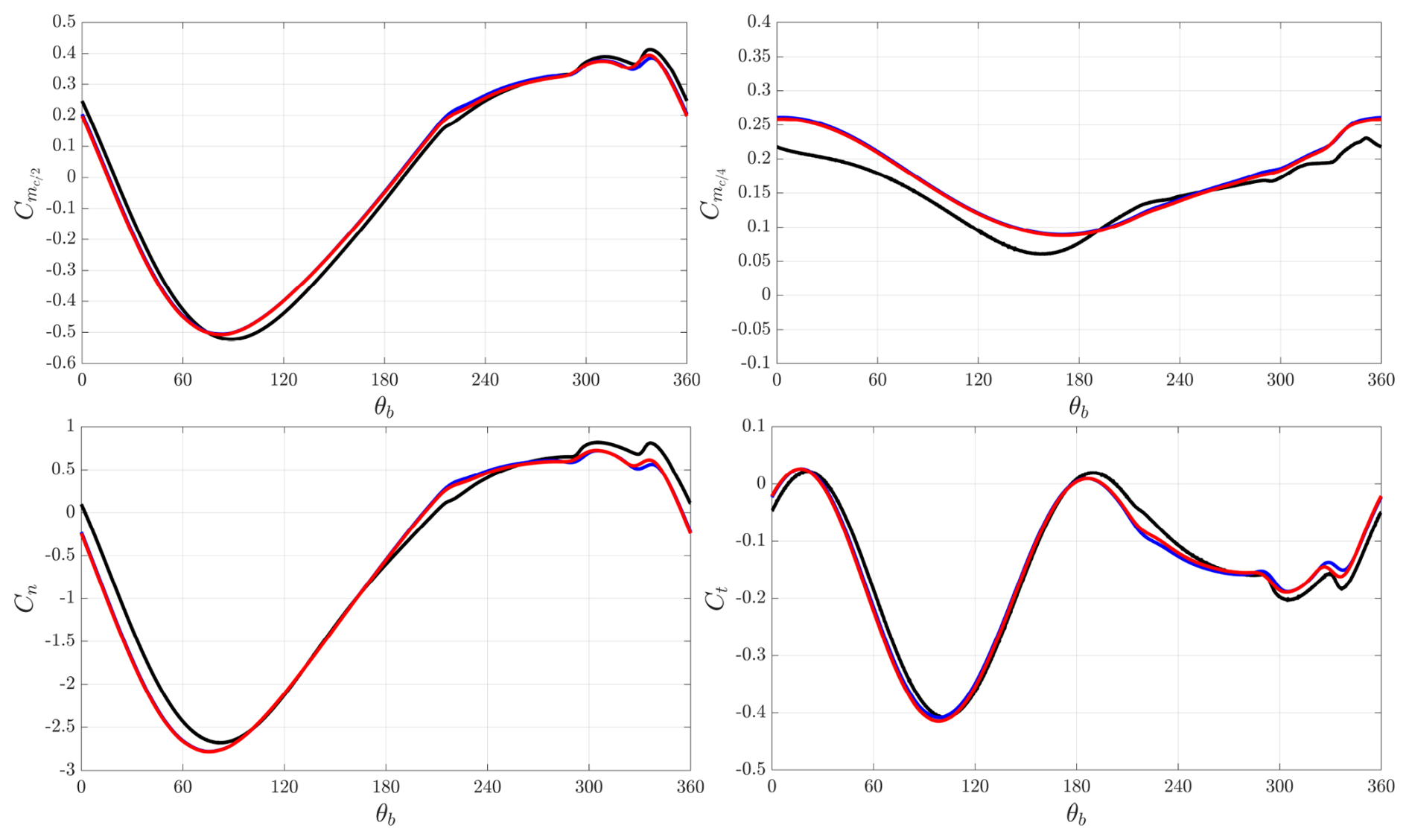
Figure 14 VAT with NACA0015 airfoil attached at $x_{\mathrm{p}}=c/\mathrm{2}$ and operating at TSR=3.25: comparison between the ALM with $m_{c/\mathrm{4}}$, $f_{\mathrm{t}}^{\mathrm{i}}$ and $f_{\mathrm{n}}^i$ explicitly enforced (red), the ALM without $m_{c/\mathrm{4}}$, $f_{\mathrm{t}}^{\mathrm{i}}$ and $f_{\mathrm{n}}^i$ explicitly enforced (blue) and the reference wall-resolved simulation (black) of $C_{m_{c/\mathrm{2}}}$, $C_{m_{c/\mathrm{4}}}$, C_n and C_t. Both ALM cases are centered at $c/\mathrm{4}$.

6.1 Case of airfoil attached at $x_{\mathrm{p}}=c/\mathrm{4}$

We first consider the case in which the airfoil is attached to the arm at its quarter-chord.

The velocity vector v of the flow is measured at $x_{\mathrm{p}}=c/\mathrm{4}$ using the integral sampling; its components are (v_t,v_n). The components of the apparent velocity vector V as seen by the rotating blade are thus $(V_{\mathrm{t}}=\mathrm{\Omega }R+v_{\mathrm{t}},V_{\mathrm{n}}=v_{\mathrm{n}})$. The angle of the velocity vector V relative to the airfoil chord is denoted α.

The mesh used for the ALM simulations is shown in Fig. 9. A rectangular domain is used, identical to that of the wall-resolved reference case. An overset technique is implemented to maintain a hexahedral mesh with the same template for the ALM ($h=\mathit{\sigma }/\mathrm{2}$) as used in Sects. 4 and 5. The overset approach also enables the rotation of the actuation zone. Two refinement regions are used: one for the turbine region, including the template, and another one for the wake. The cell size within the turbine region is chosen so as to ensure accurate interpolation between the region and the background mesh. Notably, the wall-resolved reference case mesh is more refined (≃328 000 cells) compared to the ALM mesh (≃37 000 cells), in line with the intended efficiency of the ALM approach. The methodology is applied to all ALM cases in this work.

6.1.1 Case without explicitly enforcing $m_{c/\mathrm{4}}$ and $f_{\mathrm{t}}^{\mathrm{i}}$ in the ALM

We first consider the case where we do not explicitly enforce the moment $m_{c/\mathrm{4}}$ in the ALM; hence we also cannot enforce the inviscid tangential force $f_{\mathrm{t}}^{\mathrm{i}}$ in the ALM. Only the lift and parasitic drag contributions are enforced.

The velocity vector is first corrected to compensate for the velocity induced by the shed vortex wake produced by the parasitic drag. As this wake is assumed to be shed in the direction of V, we correct its amplitude:

$$\begin{array}{}\text{(68)}& {\mathit{V}}^{\text{corr}}={\displaystyle \frac{\mathit{V}}{\left(\mathrm{1}-\frac{\mathrm{1}}{\mathrm{4}\sqrt{\mathit{\pi }}}\frac{c}{\mathit{\sigma }}{C}_{\mathrm{d}}^{\mathit{\nu }}\right)}}.\end{array}$$

The angle that the corrected velocity vector makes relative to the chord is therefore still α.

In terms of modeling, the lift force (i.e., force in the direction orthogonal to the apparent velocity) exerted by the velocity V^corr on the airfoil attached at $x_{\mathrm{p}}=c/\mathrm{4}$ and without pitch is equivalent to the normal force (= lift force) exerted by a horizontal flow of velocity V^corr on the airfoil attached at $x_{\mathrm{p}}=c/\mathrm{4}$ and pitched at an angle α_p=α. The lift coefficient is thus modeled using

$$\begin{array}{}\text{(69)}& C_{\mathrm{l}}\left(\mathit{\alpha }\right)\simeq C_{\mathrm{l}}^{\mathrm{u}}(\mathit{\alpha }-{\mathit{\alpha }}_{\mathrm{c}})-C_{\mathrm{l}}^{\mathrm{u}}\left({\mathit{\alpha }}_{\mathrm{c}}\right).\end{array}$$

Likewise, the parasitic drag (i.e., force in the direction of the apparent velocity) is modeled using

$$\begin{array}{}\text{(70)}& C_{\mathrm{d}}^{\mathit{\nu }}\left(\mathit{\alpha }\right)=C_{\mathrm{d}}^{\mathit{\nu },\mathrm{p}}\left(\mathit{\alpha }\right)+C_{\mathrm{d}}^{\mathit{\nu },\mathrm{f}}\left(\mathit{\alpha }\right)\simeq C_{\mathrm{d}}^{\text{u,p}}(\mathit{\alpha }-{\mathit{\alpha }}_{\mathrm{c}})+C_{\mathrm{d}}^{\text{u,f}}\left(\mathit{\alpha }\right).\end{array}$$

for the parasitic drag coefficient.

The moment coefficients can also be estimated. For the moment coefficient at mid-chord, the model gives

$$\begin{array}{}\text{(71)}& C_{m_{c/\mathrm{2}}}\left(\mathit{\alpha }\right)=C_{m_{c/\mathrm{2}}}^{\mathrm{0}}+{\displaystyle \frac{\mathrm{1}}{\mathrm{4}}}{C}_{\mathrm{l}}^{\mathrm{u}}(\mathit{\alpha }-{\mathit{\alpha }}_{\mathrm{c}})\cos (\mathit{\alpha }-{\mathit{\alpha }}_{\mathrm{c}}).\end{array}$$

The moment coefficient $C_{m_{c/\mathrm{4}}}$ is then also obtained as

$$\begin{array}{}\text{(72)}& \begin{array}{rl}{\displaystyle }{C}_{m_{c/\mathrm{4}}}\left(\mathit{\alpha }\right)=& {\displaystyle }{C}_{m_{c/\mathrm{2}}}\left(\mathit{\alpha }\right)-{\displaystyle \frac{\mathrm{1}}{\mathrm{4}}}{C}_{\mathrm{l}}\left(\mathit{\alpha }\right)\cos (\mathit{\alpha }-{\mathit{\alpha }}_{\mathrm{c}})\\ {\displaystyle }\simeq & {\displaystyle }{C}_{m_{c/\mathrm{2}}}^{\mathrm{0}}+{\displaystyle \frac{\mathrm{1}}{\mathrm{4}}}{C}_{\mathrm{l}}^{\mathrm{u}}\left({\mathit{\alpha }}_{\mathrm{c}}\right)\cos (\mathit{\alpha }-{\mathit{\alpha }}_{\mathrm{c}}).\end{array}\end{array}$$

Further adding the inviscid tangential force coefficient $C_{\mathrm{t}}^{\mathrm{i}}=-\frac{c}{R}{C}_{m_{c/\mathrm{4}}}$, we finally obtain

$$\begin{array}{}\text{(73)}& \begin{array}{rl}{\displaystyle }{C}_{\mathrm{t}}\left(\mathit{\alpha }\right)=& {\displaystyle }\left(C_{\mathrm{d}}^{\mathit{\nu }}\left(\mathit{\alpha }\right)\cos \left(\mathit{\alpha }\right)-C_{\mathrm{l}}\left(\mathit{\alpha }\right)\sin \left(\mathit{\alpha }\right)\right)-{\displaystyle \frac{c}{R}}{C}_{m_{c/\mathrm{4}}}\left(\mathit{\alpha }\right)\\ {\displaystyle }=& {\displaystyle }\left(C_{\mathrm{d}}^{\mathit{\nu },\mathrm{p}}\left(\mathit{\alpha }\right)\cos \left(\mathit{\alpha }\right)-C_{\mathrm{l}}\left(\mathit{\alpha }\right)\sin \left(\mathit{\alpha }\right)-{\displaystyle \frac{c}{R}}{C}_{m_{c/\mathrm{4}}}\left(\mathit{\alpha }\right)\right)\\ {\displaystyle }& {\displaystyle }+C_{\mathrm{d}}^{\mathit{\nu },\mathrm{f}}\left(\mathit{\alpha }\right)\cos \left(\mathit{\alpha }\right),\\ {\displaystyle }{C}_{\mathrm{n}}\left(\mathit{\alpha }\right)=& {\displaystyle }{C}_{\mathrm{d}}^{\mathit{\nu }}\left(\mathit{\alpha }\right)\sin \left(\mathit{\alpha }\right)+C_{\mathrm{l}}\left(\mathit{\alpha }\right)\cos \left(\mathit{\alpha }\right)\\ {\displaystyle }=& {\displaystyle }\left(C_{\mathrm{d}}^{\mathit{\nu },\mathrm{p}}\left(\mathit{\alpha }\right)\sin \left(\mathit{\alpha }\right)+C_{\mathrm{l}}\left(\mathit{\alpha }\right)\cos \left(\mathit{\alpha }\right)\right)+C_{\mathrm{d}}^{\mathit{\nu },\mathrm{f}}\left(\mathit{\alpha }\right)\sin \left(\mathit{\alpha }\right).\end{array}\end{array}$$

We have intentionally split each term into pressure and friction contributions. The net forces f_t and f_n (each split in pressure and friction contributions) and the moments, $m_{c/\mathrm{2}}$ and $m_{c/\mathrm{4}}$, are then finally obtained using V^corr, c and ρ. They can be compared to the values measured in CFD.

As we here do not explicitly impose $m_{c/\mathrm{4}}$ in the ALM, we also do not impose $f_{\mathrm{t}}^{\mathrm{i}}$. The tangential force that we impose in the ALM is hence simply the tangential projection of the lift and parasitic drag forces.

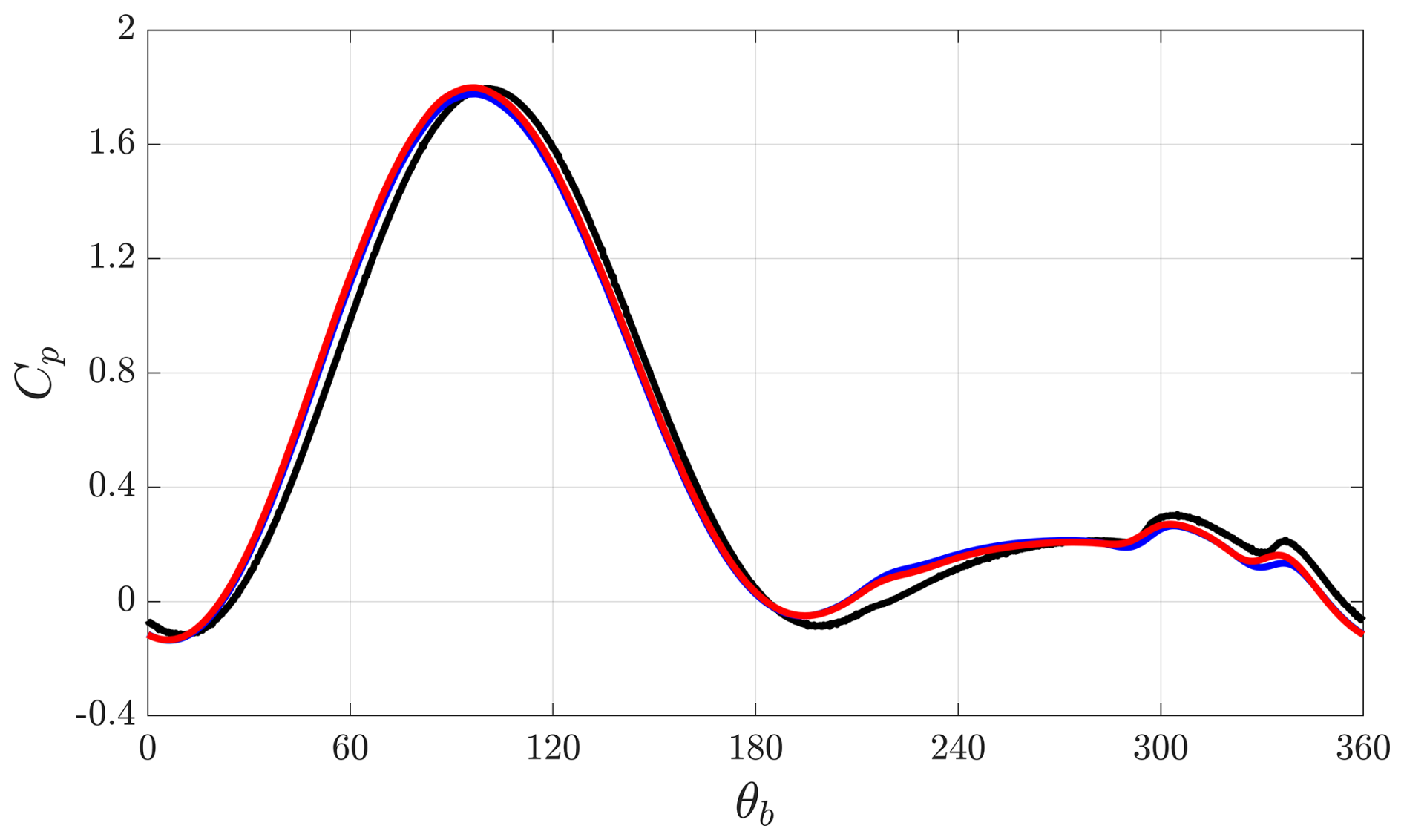
Figure 15 VAT with NACA0015 airfoil attached at $x_{\mathrm{p}}=c/\mathrm{2}$ and operating at TSR=3.25: comparison between the results of the ALM with $m_{c/\mathrm{4}}$, $f_{\mathrm{t}}^{\mathrm{i}}$ and $f_{\mathrm{n}}^i$explicitly enforced (red), the ALM without $m_{c/\mathrm{4}}$, $f_{\mathrm{t}}^{\mathrm{i}}$ and $f_{\mathrm{n}}^i$ explicitly enforced (blue) and the reference wall-resolved simulation (black) of C_p. Both ALM cases are centered at $c/\mathrm{4}$.

6.1.2 Case with explicitly enforcing $m_{c/\mathrm{4}}$ and $f_{\mathrm{t}}^{\mathrm{i}}$ in the ALM

We next consider the case where we explicitly impose $m_{c/\mathrm{4}}$ in the ALM (using the procedure developed in Sect. 5); hence we also include the contribution of $f_{\mathrm{t}}^{\mathrm{i}}$ in the imposition of the tangential force.

The values of C_l, C_d, $C_{m_{c/\mathrm{4}}}$ and $C_{\mathrm{t}}^{\mathrm{i}}$ are the same as those obtained in the above section.

Here, however, the velocity vector V must be corrected to compensate for the velocity induced by the shed vortex wake produced by the total net force imposed in the direction of V, thus including the projection of $f_{\mathrm{t}}^{\mathrm{i}}$ in this direction (as it will also shed some vorticity into the wake, even though this vorticity is not present in the real flow). The correction is thus

$$\begin{array}{}\text{(74)}& {\mathit{V}}^{\text{corr}}={\displaystyle \frac{\mathit{V}}{\left(\mathrm{1}-\frac{\mathrm{1}}{\mathrm{4}\sqrt{\mathit{\pi }}}\frac{c}{\mathit{\sigma }}\left(C_{\mathrm{d}}^{\mathit{\nu }}+C_{\mathrm{t}}^{\mathrm{i}}\cos \left(\mathit{\alpha }\right)\right)\right)}}.\end{array}$$

6.1.3 Results and comparison

We present the results of both types of simulations using ALM in Figs. 10–11 and in Table 3. The normalization used here is different from that used for the airfoil in rotation: here, the forces f_n and f_t are normalized using the wind velocity U_w and the turbine diameter D=2 R, thus using $\frac{\mathrm{1}}{\mathrm{2}}\mathit{\rho }{U}_w^{\mathrm{2}}D$. To normalize the moments $m_{c/\mathrm{4}}$ and $m_{c/\mathrm{4}}$, we use $\frac{\mathrm{1}}{\mathrm{2}}\mathit{\rho }{U}_w^{\mathrm{2}}Dc$. As for the power coefficient C_p of the VAT, it is obtained using

$$\begin{array}{}\text{(75)}& C_p=-{\displaystyle \frac{(f_{\mathrm{t}}R+m_{c/\mathrm{4}})\mathrm{\Omega }}{\frac{\mathrm{1}}{\mathrm{2}}\mathit{\rho }{U}_w^{\mathrm{3}}D}}.\end{array}$$

It is also interesting to compare the ALM-predicted contributions of pressure and friction to the tangential force f_t with those from the wall-resolved simulation. Given that the two ALM cases should be similar, we chose to perform the comparison only for the ALM with $m_{c/\mathrm{4}}$ and $f_{\mathrm{t}}^{\mathrm{i}}$ explicitly enforced; see Fig. 12.

Finally, the vorticity fields from the ALM methods are also compared to that of the wall-resolved simulation in Fig. 13.

Table 4 Mean $C_{m_{c/\mathrm{2}}}$, $C_{m_{c/\mathrm{4}}}$, C_n, C_t and C_p over a blade cycle for a VAT with airfoil attached at $x_{\mathrm{p}}=c/\mathrm{2}$ and operating at TSR=3.25. Both ALM cases are centered at $c/\mathrm{4}$.

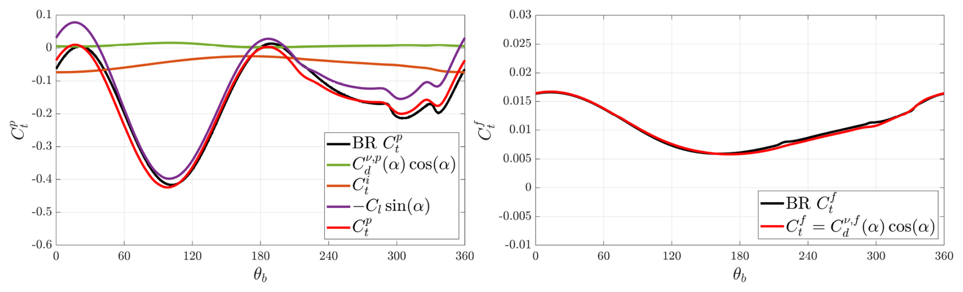
Figure 16 VAT with NACA0015 airfoil attached at $x_{\mathrm{p}}=c/\mathrm{2}$ and operating at TSR=3.25: comparison between the ALM with $m_{c/\mathrm{4}}$, $f_{\mathrm{t}}^{\mathrm{i}}$ and $f_{\mathrm{n}}^i$ explicitly enforced (red) and the reference wall-resolved simulation (black) of the pressure contribution $C_{\mathrm{t}}^{\mathrm{p}}$ (with its components) and of the friction contribution $C_{\mathrm{t}}^f$ to the tangential force coefficient. The ALM is centered at $c/\mathrm{4}$.

6.2 Case of airfoil attached at $x_{\mathrm{p}}=c/\mathrm{2}$

We consider next the case where the blade is attached to the arm at $x_{\mathrm{p}}=c/\mathrm{2}$, again without pitch.

6.2.1 Case with ALM centered at $c/\mathrm{4}$

In the usual case where the ALM is strictly applied at the aerodynamic center, the airfoil attached at $x_{\mathrm{p}}=c/\mathrm{2}$ and without pitch must be considered “equivalent to the same airfoil attached at $x_{\mathrm{p}}=c/\mathrm{4}$ and with a pitch angle of α_c”.

The components of the flow velocity v measured at $c/\mathrm{4}$ are (v_t,v_n). The components of the apparent velocity vector V are thus

$$\begin{array}{}\text{(76)}& \begin{array}{rl}{\displaystyle }{V}_{\mathrm{t}}=& {\displaystyle }\mathrm{\Omega }{\displaystyle \frac{R}{\cos \left({\mathit{\alpha }}_{\mathrm{c}}\right)}}\cos \left({\mathit{\alpha }}_{\mathrm{c}}\right)+v_{\mathrm{t}}=\mathrm{\Omega }R+v_{\mathrm{t}},\\ {\displaystyle }{V}_{\mathrm{n}}=& {\displaystyle }\mathrm{\Omega }{\displaystyle \frac{R}{\cos \left({\mathit{\alpha }}_{\mathrm{c}}\right)}}\sin \left({\mathit{\alpha }}_{\mathrm{c}}\right)+v_{\mathrm{n}}=\mathrm{\Omega }R\tan \left({\mathit{\alpha }}_{\mathrm{c}}\right)+v_{\mathrm{n}},\end{array}\end{array}$$

where $R/\cos \left({\mathit{\alpha }}_{\mathrm{c}}\right)$ corresponds to the slightly extended effective arm length when considering the circle passing through this point.

The angle of the velocity vector V relative to the airfoil chord is denoted α. The airfoil chord makes an angle α_c relative to the curved flow streamline considered at $c/\mathrm{4}$. The angle of the velocity vector relative to the curved flow streamline at $c/\mathrm{4}$ is thus ${\mathit{\alpha }}_{\mathrm{e}}=\mathit{\alpha }-{\mathit{\alpha }}_{\mathrm{c}}$. Again, there are then two ways of applying the ALM, and these are investigated below.

We first consider the case where we do not explicitly enforce the moment $m_{c/\mathrm{4}}$ in the ALM; hence we also cannot enforce the associated inviscid force in the ALM. Only the lift and the parasitic drag contributions will be enforced in the ALM.

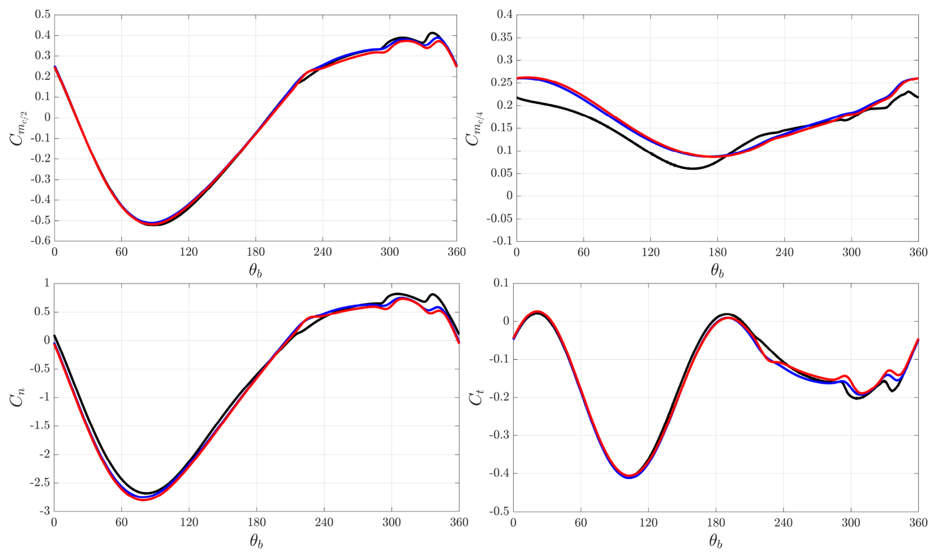
Figure 17 VAT with NACA0015 airfoil attached at $x_{\mathrm{p}}=c/\mathrm{2}$ and operating at TSR=3.25: comparison between the ALM with $m_{c/\mathrm{2}}$ and $f_{\mathrm{t}}^{\mathrm{i}}$ explicitly enforced (red), the ALM without $m_{c/\mathrm{2}}$ and $f_{\mathrm{t}}^{\mathrm{i}}$ explicitly enforced (blue) and the reference wall-resolved simulation (black) of $C_{m_{c/\mathrm{2}}}$, $C_{m_{c/\mathrm{4}}}$, C_n and C_t. Both ALM cases are centered at $x_{\mathrm{p}}=c/\mathrm{2}$.

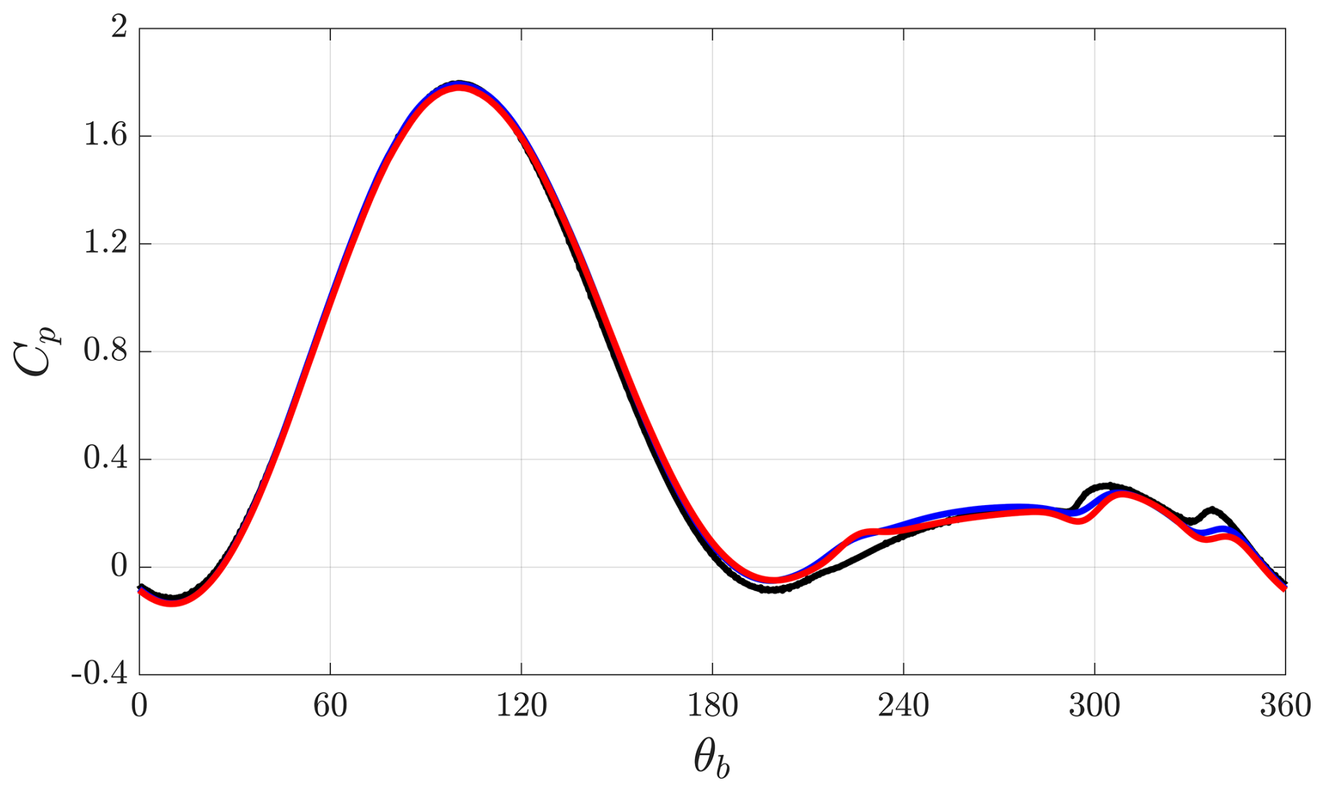
Figure 18 VAT with NACA0015 airfoil attached at $x_{\mathrm{p}}=c/\mathrm{2}$ and operating at TSR=3.25: comparison between the results of the ALM with $m_{c/\mathrm{2}}$ and $f_{\mathrm{t}}^{\mathrm{i}}$ explicitly enforced (red), the ALM without $m_{c/\mathrm{2}}$ and $f_{\mathrm{t}}^{\mathrm{i}}$ explicitly enforced (blue) and the reference wall-resolved simulation (black) of C_p. Both ALM cases are centered at $x_{\mathrm{p}}=c/\mathrm{2}$.

The amplitude of the velocity must be corrected to compensate for the velocity induced by the shed vortex wake produced by the parasitic drag:

$$\begin{array}{}\text{(77)}& {\mathit{V}}^{\text{corr}}={\displaystyle \frac{\mathit{V}}{\left(\mathrm{1}-\frac{\mathrm{1}}{\mathrm{4}\sqrt{\mathit{\pi }}}\frac{c}{\mathit{\sigma }}{C}_{\mathrm{d}}^{\mathit{\nu }}\right)}}.\end{array}$$

The angle of this corrected velocity vector relative to the curved flow streamline at $c/\mathrm{4}$ is therefore still α−α_c.

In terms of modeling, the lift force (i.e., force in the direction orthogonal to the apparent velocity) exerted by the velocity V^corr on the airfoil attached at $c/\mathrm{4}$ and with pitch α_c is equivalent to the normal force (= also lift force) exerted by a horizontal flow of velocity V^corr on the airfoil attached at $c/\mathrm{4}$ and pitched by an angle ${\mathit{\alpha }}_{\mathrm{p}}={\mathit{\alpha }}_{\mathrm{e}}+{\mathit{\alpha }}_{\mathrm{c}}$. The lift coefficient is thus modeled using

$$\begin{array}{}\text{(78)}& \begin{array}{rl}{\displaystyle }{C}_{\mathrm{l}}\left(\mathit{\alpha }\right)\simeq & {\displaystyle }{C}_{\mathrm{l}}^{\mathrm{u}}\left(\right({\mathit{\alpha }}_{\mathrm{e}}+{\mathit{\alpha }}_{\mathrm{c}})-{\mathit{\alpha }}_{\mathrm{c}})-C_{\mathrm{l}}^{\mathrm{u}}\left({\mathit{\alpha }}_{\mathrm{c}}\right)\\ {\displaystyle }=& {\displaystyle }{C}_{\mathrm{l}}^{\mathrm{u}}(\mathit{\alpha }-{\mathit{\alpha }}_{\mathrm{c}})-C_{\mathrm{l}}^{\mathrm{u}}\left({\mathit{\alpha }}_{\mathrm{c}}\right).\end{array}\end{array}$$

Likewise, the parasitic drag (i.e., force in the direction of the apparent velocity) is modeled using

$$\begin{array}{}\text{(79)}& \begin{array}{rl}{\displaystyle }{C}_{\mathrm{d}}^{\mathit{\nu }}\left(\mathit{\alpha }\right)=& {\displaystyle }{C}_{\mathrm{d}}^{\mathit{\nu },\mathrm{p}}\left(\mathit{\alpha }\right)+C_{\mathrm{d}}^{\mathit{\nu },\mathrm{f}}\left(\mathit{\alpha }\right)\\ {\displaystyle }\simeq & {\displaystyle }{C}_{\mathrm{d}}^{\text{u,p}}(\mathit{\alpha }-{\mathit{\alpha }}_{\mathrm{c}})+C_{\mathrm{d}}^{\text{u,f}}\left(\mathit{\alpha }\right).\end{array}\end{array}$$

These expressions are the same as those obtained for the case where the airfoil was attached at $x_{\mathrm{p}}=c/\mathrm{4}$. This makes sense since the apparent velocity vector is that considered at $c/\mathrm{4}$ in both cases and since the angle α of this vector is defined relative to the airfoil chord in both cases. The only difference lies in the apparent velocity vector; see Eq. (76).

The models for the moment coefficients are also identical:

$$\begin{array}{}\text{(80)}& C_{m_{c/\mathrm{2}}}\left(\mathit{\alpha }\right)=C_{m_{c/\mathrm{2}}}^{\mathrm{0}}+{\displaystyle \frac{\mathrm{1}}{\mathrm{4}}}{C}_{\mathrm{l}}^{\mathrm{u}}(\mathit{\alpha }-{\mathit{\alpha }}_{\mathrm{c}})\cos (\mathit{\alpha }-{\mathit{\alpha }}_{\mathrm{c}})\end{array}$$

and

$$\begin{array}{}\text{(81)}& \begin{array}{rl}{\displaystyle }{C}_{m_{c/\mathrm{4}}}\left(\mathit{\alpha }\right)=& {\displaystyle }{C}_{m_{c/\mathrm{2}}}\left(\mathit{\alpha }\right)-{\displaystyle \frac{\mathrm{1}}{\mathrm{4}}}{C}_{\mathrm{l}}\left(\mathit{\alpha }\right)\cos (\mathit{\alpha }-{\mathit{\alpha }}_{\mathrm{c}})\\ {\displaystyle }\simeq & {\displaystyle }{C}_{m_{c/\mathrm{2}}}^{\mathrm{0}}+{\displaystyle \frac{\mathrm{1}}{\mathrm{4}}}{C}_{\mathrm{l}}^{\mathrm{u}}\left({\mathit{\alpha }}_{\mathrm{c}}\right)\cos (\mathit{\alpha }-{\mathit{\alpha }}_{\mathrm{c}}).\end{array}\end{array}$$

The coefficient for the inviscid force on the airfoil “as if it were attached at $c/\mathrm{4}$” still counterbalances the moment $m_{c/\mathrm{4}}$. This inviscid force now acts in the direction of α_c, and thus we obtain $C_{\mathrm{t}}^{\mathrm{i}}=-\frac{c}{R}{C}_{m_{c/\mathrm{4}}}\cos \left({\mathit{\alpha }}_{\mathrm{c}}\right)$ and $C_{\mathrm{n}}^i=-\frac{c}{R}{C}_{m_{c/\mathrm{4}}}\sin \left({\mathit{\alpha }}_{\mathrm{c}}\right)$. We finally obtain

$$\begin{array}{}\text{(82)}& \begin{array}{rl}{\displaystyle }& {\displaystyle }{C}_{\mathrm{t}}\left(\mathit{\alpha }\right)\\ {\displaystyle }& {\displaystyle }=\left(C_{\mathrm{d}}^{\mathit{\nu }}\left(\mathit{\alpha }\right)\cos \left(\mathit{\alpha }\right)-C_{\mathrm{l}}\left(\mathit{\alpha }\right)\sin \left(\mathit{\alpha }\right)\right)-{\displaystyle \frac{c}{R}}{C}_{m_{c/\mathrm{4}}}\left(\mathit{\alpha }\right)\cos \left({\mathit{\alpha }}_{\mathrm{c}}\right)\\ {\displaystyle }& {\displaystyle }=\left(C_{\mathrm{d}}^{\mathit{\nu },\mathrm{p}}\left(\mathit{\alpha }\right)\cos \left(\mathit{\alpha }\right)-C_{\mathrm{l}}\left(\mathit{\alpha }\right)\sin \left(\mathit{\alpha }\right)-{\displaystyle \frac{c}{R}}{C}_{m_{c/\mathrm{4}}}\cos \left({\mathit{\alpha }}_{\mathrm{c}}\right)\right)\\ {\displaystyle }& {\displaystyle }+C_{\mathrm{d}}^{\mathit{\nu },\mathrm{f}}\left(\mathit{\alpha }\right)\cos \left(\mathit{\alpha }\right),\\ {\displaystyle }& {\displaystyle }{C}_{\mathrm{n}}\left(\mathit{\alpha }\right)\\ {\displaystyle }& {\displaystyle }=\left(C_{\mathrm{d}}^{\mathit{\nu }}\left(\mathit{\alpha }\right)\sin \left(\mathit{\alpha }\right)+C_{\mathrm{l}}\left(\mathit{\alpha }\right)\cos \left(\mathit{\alpha }\right)\right)-{\displaystyle \frac{c}{R}}{C}_{m_{c/\mathrm{4}}}\left(\mathit{\alpha }\right)\sin \left({\mathit{\alpha }}_{\mathrm{c}}\right)\\ {\displaystyle }& {\displaystyle }=\left(C_{\mathrm{d}}^{\mathit{\nu },\mathrm{p}}\left(\mathit{\alpha }\right)\sin \left(\mathit{\alpha }\right)+C_{\mathrm{l}}\left(\mathit{\alpha }\right)\cos \left(\mathit{\alpha }\right)-{\displaystyle \frac{c}{R}}{C}_{m_{c/\mathrm{4}}}\left(\mathit{\alpha }\right)\sin \left({\mathit{\alpha }}_{\mathrm{c}}\right)\right)\\ {\displaystyle }& {\displaystyle }+C_{\mathrm{d}}^{\mathit{\nu },\mathrm{f}}\left(\mathit{\alpha }\right)\sin \left(\mathit{\alpha }\right).\end{array}\end{array}$$

When we do not explicitly impose $m_{c/\mathrm{4}}$ in the ALM, we also do not impose $f_{\mathrm{t}}^{\mathrm{i}}$ and $f_{\mathrm{n}}^i$.

When we explicitly enforce $m_{c/\mathrm{4}}$ in the ALM, we must also explicitly enforce $f_{\mathrm{t}}^{\mathrm{i}}$ and $f_{\mathrm{n}}^i$. The correction of the measured velocity V must now also account for the component of the inviscid force in this direction:

$$\begin{array}{}\text{(83)}& {\mathit{V}}^{\text{corr}}={\displaystyle \frac{\mathit{V}}{\left(\mathrm{1}-\frac{\mathrm{1}}{\mathrm{4}\sqrt{\mathit{\pi }}}\frac{c}{\mathit{\sigma }}\left(C_{\mathrm{d}}^{\mathit{\nu }}+C_{\mathrm{t}}^{\mathrm{i}}\cos (\mathit{\alpha }-{\mathit{\alpha }}_{\mathrm{c}})\right)\right)}}.\end{array}$$

We present the results of both types of simulations using the ALM centered at $c/\mathrm{4}$ in Figs. 14–16 and in Table 4.

Table 5 Mean $C_{m_{c/\mathrm{2}}}$, $C_{m_{c/\mathrm{4}}}$, C_n, C_t and C_p over a blade cycle for the three cases studied of a VAT at TSR=3.25 with the blade attached at $x_{\mathrm{p}}=c/\mathrm{2}$. Both ALM cases are centered at $x_{\mathrm{p}}=c/\mathrm{2}$.

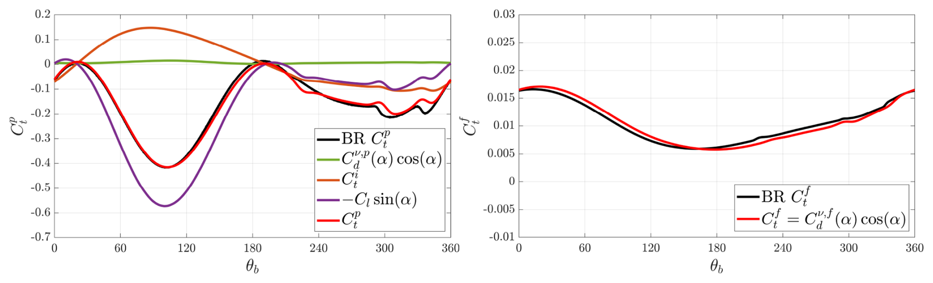
Figure 19 VAT with NACA0015 airfoil attached at $x_{\mathrm{p}}=c/\mathrm{2}$ and operating at TSR=3.25: comparison between the ALM with $m_{c/\mathrm{2}}$ and $f_{\mathrm{t}}^{\mathrm{i}}$ explicitly enforced (red) and the reference wall-resolved simulation (black) of the pressure contribution $C_{\mathrm{t}}^{\mathrm{p}}$ (with its components) and of the friction contribution $C_{\mathrm{t}}^f$ to the tangential force coefficient. The ALM is centered at $x_{\mathrm{p}}=c/\mathrm{2}$.

6.2.2 Case with ALM centered at $c/\mathrm{2}$

One could however also consider that an ALM can be used as a model to represent the airfoil at its attachment point, thus centering the ALM at $x_{\mathrm{p}}=c/\mathrm{2}$. In this case, we also measure the flow velocity vector v at $x_{\mathrm{p}}=c/\mathrm{2}$: its components are (v_t,v_n). The components of the apparent velocity vector V are thus $(V_{\mathrm{t}}=\mathrm{\Omega }R+v_{\mathrm{t}},V_{\mathrm{n}}=v_{\mathrm{n}})$. The angle it makes relative to the airfoil chord is α.

In terms of modeling, the force exerted in the direction orthogonal to the apparent velocity V^corr on the airfoil attached at $x_{\mathrm{p}}=c/\mathrm{2}$ and without pitch is equivalent to the normal force exerted by a horizontal flow of velocity V^corr on the airfoil attached at $x_{\mathrm{p}}=c/\mathrm{2}$ and pitched by an angle α_p=α; the parasitic force exerted in the direction parallel to the apparent velocity is equivalent to the parasitic tangential force exerted by a horizontal flow of velocity V^corr on the airfoil pitched by an angle α_p=α. The related force coefficients are thus modeled using

$$\begin{array}{}\text{(84)}& \begin{array}{rl}{\displaystyle }{C}_{⟂}\left(\mathit{\alpha }\right)=& {\displaystyle }{C}_{\mathrm{l}}^{\mathrm{u}}\left(\mathit{\alpha }\right)-C_{\mathrm{l}}^{\mathrm{u}}\left({\mathit{\alpha }}_{\mathrm{c}}\right),\\ {\displaystyle }{C}_{\parallel }\left(\mathit{\alpha }\right)=& {\displaystyle }{C}_{\mathrm{d}}^{\text{u,p}}\left(\mathit{\alpha }\right)+C_{\mathrm{d}}^{\text{u,f}}(\mathit{\alpha }+{\mathit{\alpha }}_{\mathrm{c}}).\end{array}\end{array}$$

The normal and tangential components are hence obtained as

$$\begin{array}{}\text{(85)}& \begin{array}{rl}{\displaystyle }{C}_{\mathrm{n}}\left(\mathit{\alpha }\right)=& {\displaystyle }{C}_{⟂}\left(\mathit{\alpha }\right)\cos \left(\mathit{\alpha }\right)+C_{\parallel }\left(\mathit{\alpha }\right)\sin \left(\mathit{\alpha }\right),\\ {\displaystyle }{C}_{\mathrm{t}}\left(\mathit{\alpha }\right)=& {\displaystyle }{C}_{\parallel }\left(\mathit{\alpha }\right)\cos \left(\mathit{\alpha }\right)-C_{⟂}\left(\mathit{\alpha }\right)\sin \left(\mathit{\alpha }\right).\end{array}\end{array}$$

The corrected velocity vector is

$$\begin{array}{}\text{(86)}& {\mathit{V}}^{\text{corr}}={\displaystyle \frac{\mathit{V}}{\left(\mathrm{1}-\frac{\mathrm{1}}{\mathrm{4}\sqrt{\mathit{\pi }}}\frac{c}{\mathit{\sigma }}{C}_{\parallel }\right)}}.\end{array}$$

The angle that V^corr makes relative to the curved flow streamline at the location of the aerodynamic center is ${\mathit{\alpha }}_{\mathrm{e}}=\mathit{\alpha }-{\mathit{\alpha }}_{\mathrm{c}}$. The moment $m_{c/\mathrm{4}}$ is hence obtained as

$$\begin{array}{}\text{(87)}& C_{m_{c/\mathrm{4}}}\left(\mathit{\alpha }\right)\simeq C_{m_{c/\mathrm{2}}}^{\mathrm{0}}+{\displaystyle \frac{\mathrm{1}}{\mathrm{4}}}{C}_{\mathrm{l}}^{\mathrm{u}}\left({\mathit{\alpha }}_{\mathrm{c}}\right)\cos (\mathit{\alpha }-{\mathit{\alpha }}_{\mathrm{c}}).\end{array}$$

The moment coefficient $C_{m_{c/\mathrm{2}}}$ is thus obtained as

$$\begin{array}{}\text{(88)}& C_{m_{c/\mathrm{2}}}\left(\mathit{\alpha }\right)\simeq C_{m_{c/\mathrm{4}}}+{\displaystyle \frac{\mathrm{1}}{\mathrm{4}}}{C}_{\mathrm{n}}\left(\mathit{\alpha }\right).\end{array}$$

The associated inviscid tangential force is then $f_{\mathrm{t}}^{\mathrm{i}}=-m_{c/\mathrm{2}}/R$, thus with coefficient

$$\begin{array}{}\text{(89)}& C_{\mathrm{t}}^{\mathrm{i}}\left(\mathit{\alpha }\right)=-{\displaystyle \frac{c}{R}}{C}_{m_{c/\mathrm{2}}}\left(\mathit{\alpha }\right).\end{array}$$

If we do not explicitly enforce the moment $m_{c/\mathrm{2}}$ in the ALM, we also do not enforce $f_{\mathrm{t}}^{\mathrm{i}}$. We then only enforce the normal and tangential forces associated with C_n and C_t of Eq. (85).

If we explicitly enforce the moment $m_{c/\mathrm{2}}$ in the ALM, we must also enforce $f_{\mathrm{t}}^{\mathrm{i}}$; hence the component $C_{\mathrm{t}}^{\mathrm{i}}\left(\mathit{\alpha }\right)$ must be added to the formula for C_t in Eq. (85). The corrected velocity vector must also be modified:

$$\begin{array}{}\text{(90)}& {\mathit{V}}^{\text{corr}}={\displaystyle \frac{\mathit{V}}{\left(\mathrm{1}-\frac{\mathrm{1}}{\mathrm{4}\sqrt{\mathit{\pi }}}\frac{c}{\mathit{\sigma }}\left(C_{\parallel }+C_{\mathrm{t}}^{\mathrm{i}}\cos \left(\mathit{\alpha }\right)\right)\right)}}.\end{array}$$

We present the results of both type of simulations using the ALM centered at $x_{\mathrm{p}}=c/\mathrm{2}$ in Figs. 17–19 and in Table 5.

In this configuration (ALM centered at $x_{\mathrm{p}}=c/\mathrm{2}$), it can be observed that the upstream prediction (0°–180°) is excellent. In fact, when the ALM is centered at $c/\mathrm{4}$, a small shift in the peak power coefficient is noticeable in the upstream part of the cycle. This shift is eliminated when using the ALM centered at $c/\mathrm{2}$. For the downstream region (180°–360°), small discrepancies persist, as the flow is disturbed by the wake of the upstream blade, making the effective angle of attack prediction more challenging.

7 Conclusions

The modeling of flow curvature effects on airfoils was further improved and implemented in an actuator line method (ALM), the rule being that such modeling can only use, as input, the aerodynamic coefficients of the airfoil in a uniform flow as a function of its angle of attack.

The basic models for the normal force and moment coefficients are not new and are obtained using the usual analogy with potential flow past an airfoil with curved streamlines. The model for the normal force was further improved here, to remain valid up to large pitch angles, even close to stall. The effect of the aerodynamic moment induced by the flow curvature is also found to be important and cannot be ignored. The curvature effects depend on both the attachment point of the airfoil to the arm and the pitch angle, and we have developed models that cover all possibilities.

The model for the tangential force is new (here, the analogy with a potential flow is flawed). The model is based on the fact that, for an airfoil attached to a rotating arm, the moment at the root of the arm must be zero if the flow is assumed inviscid. This was verified numerically by performing inviscid CFD simulations at various airfoil pitch angles. The inviscid tangential force that is compatible with the aerodynamic moment can, hence, be computed. For modeling viscous flows, we then add the parasitic drag to this inviscid tangential force.

The improved models were first validated against reference data corresponding to wall-resolved CFD of a rotating NACA0015 airfoil with $cR=\frac{\mathrm{2}}{\mathrm{7}}$ at various pitch angles, for angles up to stall and also for two attachment points of the airfoil to the arm (at mid-chord and quarter-chord).

The ALM with the improved models was then implemented in the CFD framework and used to simulate the unsteady flow corresponding to a VAT configuration: a rotating airfoil without pitch placed in a free stream at $\text{TSR}=\frac{\mathrm{\Omega }R}{U_w}=\mathrm{3.25}$. For this, a novel method was also developed to enforce the aerodynamic moment in the ALM. The various components of the ALM results were compared with those of the reference CFD data. They were found to be in good agreement throughout the rotation cycle.

It was also shown that the ALM can here be used in various ways: if one ignores the contribution of the aerodynamic moment in the ALM, then one must also ignore the inviscid part of the tangential force in the ALM; if one enforces the contribution of the moment in the ALM, then one must also enforce the inviscid part of the tangential force.

The above validations give us confidence that the proposed models, together with their implementation in an ALM simulation framework (including the new method for enforcing a moment), constitute useful simplified tools for modeling complex unsteady flows with good accuracy, such as VAT configurations where the flow curvature modifies both the normal and tangential forces and also produces an aerodynamic moment.

We stress that the normal force model is, so far, obtained using the analogy with curved potential flow past a flat plate put at some pitch angle, as developed in Appendix E. The model was however tested with good success on a NACA0015 airfoil: an airfoil that is not very thin and thus already challenges this model. Given that the ALM results obtained for the airfoil are quite good, it is likely that they would still be good when simulating a thicker airfoil, such as a NACA0018, and maybe still acceptable when simulating a NACA0021. One could also further improve the normal force model by taking into account the combined effects of flow curvature and airfoil thickness. Obtaining the exact solution of curved potential flow past a thick airfoil put at some pitch angle would constitute a good step in this direction.

We also note that the method proposed here for enforcing the aerodynamic moment in an ALM, in addition to enforcing the forces, can also be used to model unsteady flows involving cambered airfoils (thus with intrinsic aerodynamic moment), hence also VAT using cambered blades.

Finally, it is recognized that the proposed models are, so far, limited to flows without fast unsteady effects or dynamic stall. A next step in their development should focus on modeling such effects.

Appendix A: NACA0015 airfoil in uniform flow and associated aerodynamic coefficients

The aerodynamic coefficients of the NACA0015 airfoil in uniform flow were here obtained using wall-resolved CFD in RANS at $R{e}_{\mathrm{c}}=\mathrm{6.0}\times {\mathrm{10}}^{\mathrm{6}}$: a high Reynolds number case where the boundary layers are turbulent. We note that the simulation setup has also been validated against experimental data of the pressure coefficient distribution along the airfoil chord, at different spanwise location of a 3D wing, and up to near the wing tip; this is reported in Villeneuve et al. (2021).

The coefficients are denoted using a superscript “u” (which stands for “uniform” flow) so as to avoid any confusion with the coefficients measured in CFD of the rotating NACA0015 airfoil. The variation in the coefficients as a function of the angle of attack (denoted β to avoid any confusion with the notation α used for the angle of attack of a rotating airfoil) is shown in Fig. A1.

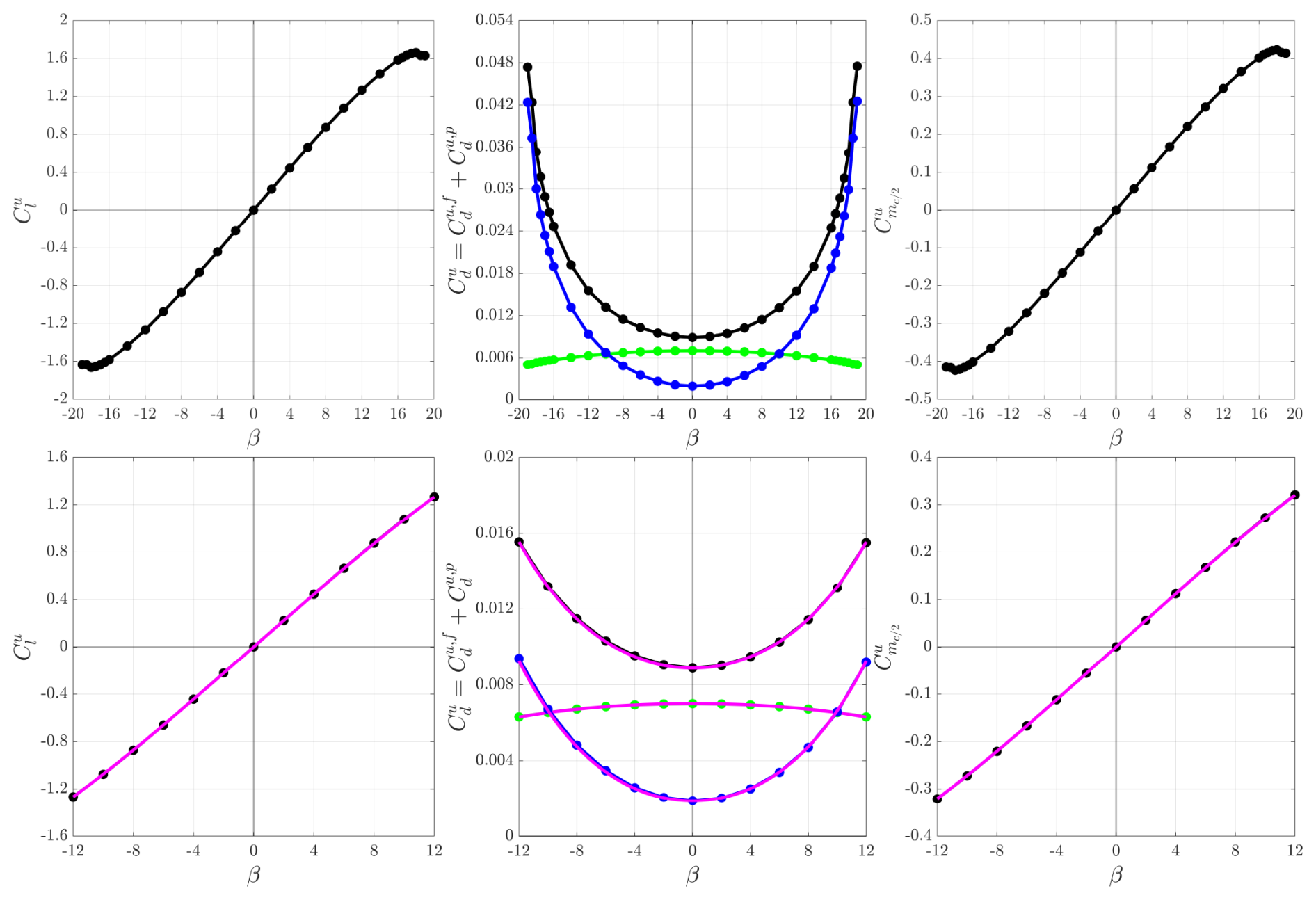
Figure A1 Coefficients $C_{\mathrm{l}}^{\mathrm{u}}$, $C_{\mathrm{d}}^{\mathrm{u}}$ (with its $C_{\mathrm{d}}^{\text{u,f}}$ (green) and $C_{\mathrm{d}}^{\text{u,p}}$ (blue) contributions) and $C_{m_{c/\mathrm{2}}}^{\mathrm{u}}$ as a function of the angle of attack β for the NACA0015 airfoil in uniform flow: data for the complete range (top), data for the range $\left|\mathit{\beta }\right|\le \mathrm{12}\mathit{°}$ (bottom) and with the mathematical fit (magenta).

For the range with $\left|\mathit{\beta }\right|\le \mathrm{12}\mathit{°}$, the lift coefficient can be fitted well using

$$\begin{array}{}\text{(A1)}& C_{\mathrm{l}}^{\mathrm{u}}\left(\mathit{\beta }\right)\simeq \mathrm{6.390}\mathit{\beta }-\mathrm{7.8}{\mathit{\beta }}^{\mathrm{3}}=\mathrm{6.390}\mathit{\beta }\left(\mathrm{1}-\mathrm{1.22}{\mathit{\beta }}^{\mathrm{2}}\right),\end{array}$$

with β in rad. The slope of 6.390 at β=0 was fitted using the CFD data at small angle ($\left|\mathit{\beta }\right|\le \mathrm{4}\mathit{°}$): it is slightly larger than 2π due to the beneficial effect of thickness (also predicted by potential flow theory). The degradation when β increases (due to parasitic viscous effects on the pressure field) is however significantly faster than that of a potential flow (where it would go as $\sin \mathit{\beta }\simeq \mathit{\beta }\left(\mathrm{1}-{\mathit{\beta }}^{\mathrm{2}}/\mathrm{6}\right)$ for small β).

Using the same procedure, the moment coefficient around the mid-chord point, $x=c/\mathrm{2}$, is fitted well using

$$\begin{array}{}\text{(A2)}& C_{m_{c/\mathrm{2}}}^{\mathrm{u}}\left(\mathit{\beta }\right)\simeq \mathrm{1.614}\mathit{\beta }-\mathrm{1.9}{\mathit{\beta }}^{\mathrm{3}}.\end{array}$$

The parasitic drag coefficient can also be fitted using

$$\begin{array}{}\text{(A3)}& C_{\mathrm{d}}^{\mathrm{u}}\left(\mathit{\beta }\right)\simeq \mathrm{0.00889}+\mathrm{0.116}{\mathit{\beta }}^{\mathrm{2}}+\mathrm{0.82}{\mathit{\beta }}^{\mathrm{4}}.\end{array}$$

Contrary to the lift and moment coefficients (where it is mostly the pressure field that contributes; the contribution due to wall friction being negligible), there are two important contributions to the parasitic drag: the friction drag and the pressure drag. Each can be fitted independently. We obtain

$$\begin{array}{}\text{(A4)}& \begin{array}{rl}{\displaystyle }{C}_{\mathrm{d}}^{\text{u,f}}\left(\mathit{\beta }\right)\simeq & {\displaystyle }\mathrm{0.00701}-\mathrm{0.014}{\mathit{\beta }}^{\mathrm{2}}-\mathrm{0.05}{\mathit{\beta }}^{\mathrm{4}},\\ {\displaystyle }{C}_{\mathrm{d}}^{\text{u,p}}\left(\mathit{\beta }\right)\simeq & {\displaystyle }\mathrm{0.00188}+\mathrm{0.130}{\mathit{\beta }}^{\mathrm{2}}+\mathrm{0.87}{\mathit{\beta }}^{\mathrm{4}}.\end{array}\end{array}$$

The friction contribution is dominant at small angles (it represents 79 % of the drag when β=0), and it decreases slowly as the angle increases. The pressure contribution is moderate at small angles, and it increases rapidly as the angle increases; it even becomes dominant beyond about 10 °.

The precise position of the aerodynamic center is then further obtained using the CFD data for $C_{\mathrm{l}}^{\mathrm{u}}\left(\mathit{\beta }\right)$ and $C_{m_{c/\mathrm{2}}}^{\mathrm{u}}\left(\mathit{\beta }\right)$ with $\left|\mathit{\beta }\right|\le \mathrm{4}\mathit{°}$, and the result is x_ac≃0.2476 c. The distance between the aerodynamic center and the mid-chord point is thus $=(\mathrm{0.5}-\mathrm{0.2476})c=\mathrm{0.2524}c$. The aerodynamic moment coefficient is then obtained using

$$\begin{array}{}\text{(A5)}& C_{m_{\text{ac}}}^{\mathrm{u}}\left(\mathit{\beta }\right)=C_{m_{c/\mathrm{2}}}^{\mathrm{u}}\left(\mathit{\beta }\right)-\mathrm{0.2524}\cos \left(\mathit{\beta }\right)C_{\mathrm{l}}^{\mathrm{u}}\left(\mathit{\beta }\right).\end{array}$$

This is shown in Fig. A2. It is indeed constant for small angles (i.e., no linear term, as it should) and it is well fitted for moderate angles using

$$\begin{array}{}\text{(A6)}& C_{m_{\text{ac}}}^{\mathrm{u}}\left(\mathit{\beta }\right)\simeq \mathrm{0.710}{\mathit{\beta }}^{\mathrm{3}}+\mathrm{2.4}{\mathit{\beta }}^{\mathrm{5}}.\end{array}$$

The moment coefficient around $x=c/\mathrm{4}$ (i.e., the approximate location of the aerodynamic center) is also shown: as expected, it is not totally flat for small angles. It can be fitted using

$$\begin{array}{}\text{(A7)}& C_{m_{c/\mathrm{4}}}^{\mathrm{u}}\left(\mathit{\beta }\right)\simeq \mathrm{0.0144}\mathit{\beta }+\mathrm{0.81}{\mathit{\beta }}^{\mathrm{3}}.\end{array}$$

The coefficient of the linear term is non-zero yet very small.

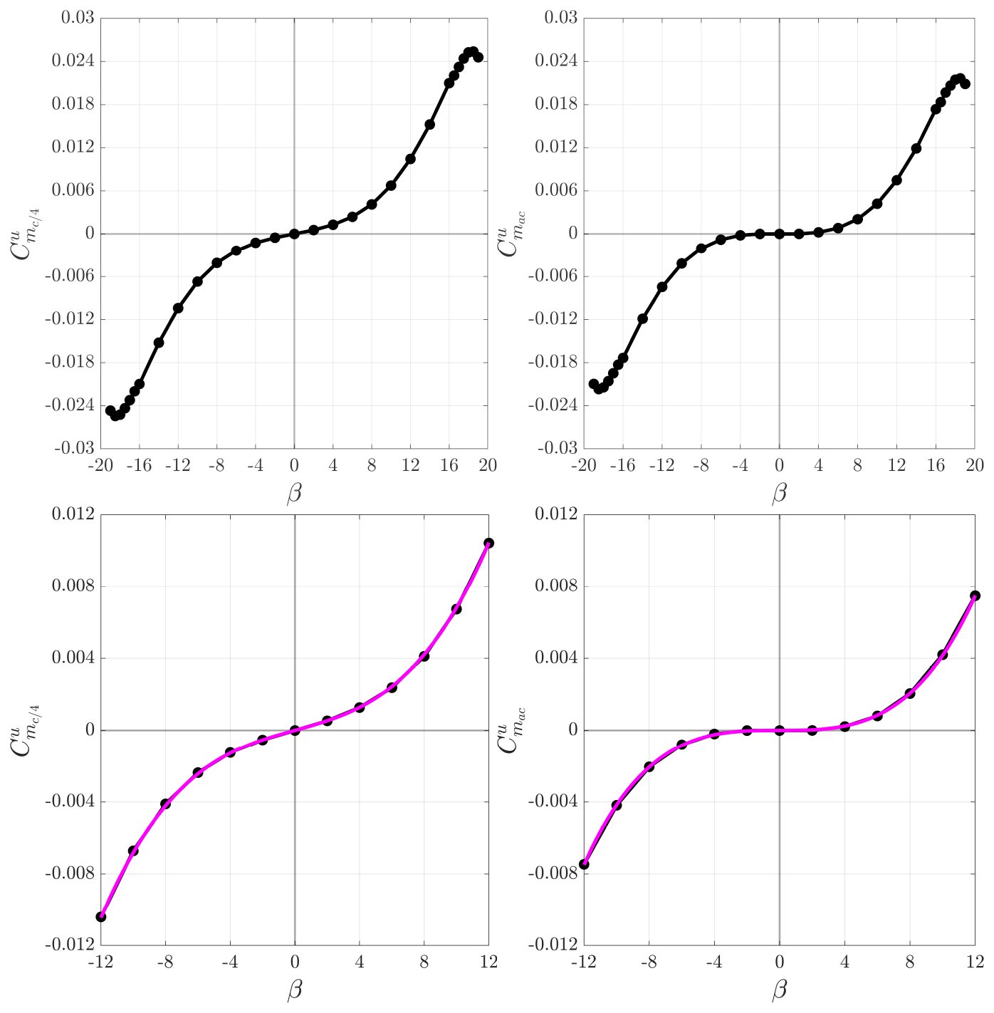
Figure A2 Coefficients $C_{m_{\text{ac}}}^{\mathrm{u}}$ and $C_{m_{c/\mathrm{4}}}^{\mathrm{u}}$ as a function of the angle of attack β: data for the complete range (top), data for the range $\left|\mathit{\beta }\right|\le \mathrm{12}\mathit{°}$ (bottom) and with the mathematical fit (magenta).

Appendix B: NACA0015 airfoil in rotation and associated aerodynamic coefficients

The NACA0015 airfoil in rotation was also simulated using wall-resolved CFD at $R{e}_{\mathrm{c}}=\mathrm{6.0}\times {\mathrm{10}}^{\mathrm{6}}$. Two cases were simulated: case with attachment point at mid-chord ($x_{\mathrm{p}}=c/\mathrm{2}$) and case with attachment point at quarter-chord ($x_{\mathrm{p}}=c/\mathrm{4}$).

B1 Simulation setup

The simulation setup, with the key-hole mesh, is shown in Fig. B1. A close-up of the body-fitted mesh is also provided. The vorticity field associated with the boundary layers and the wake is also shown.

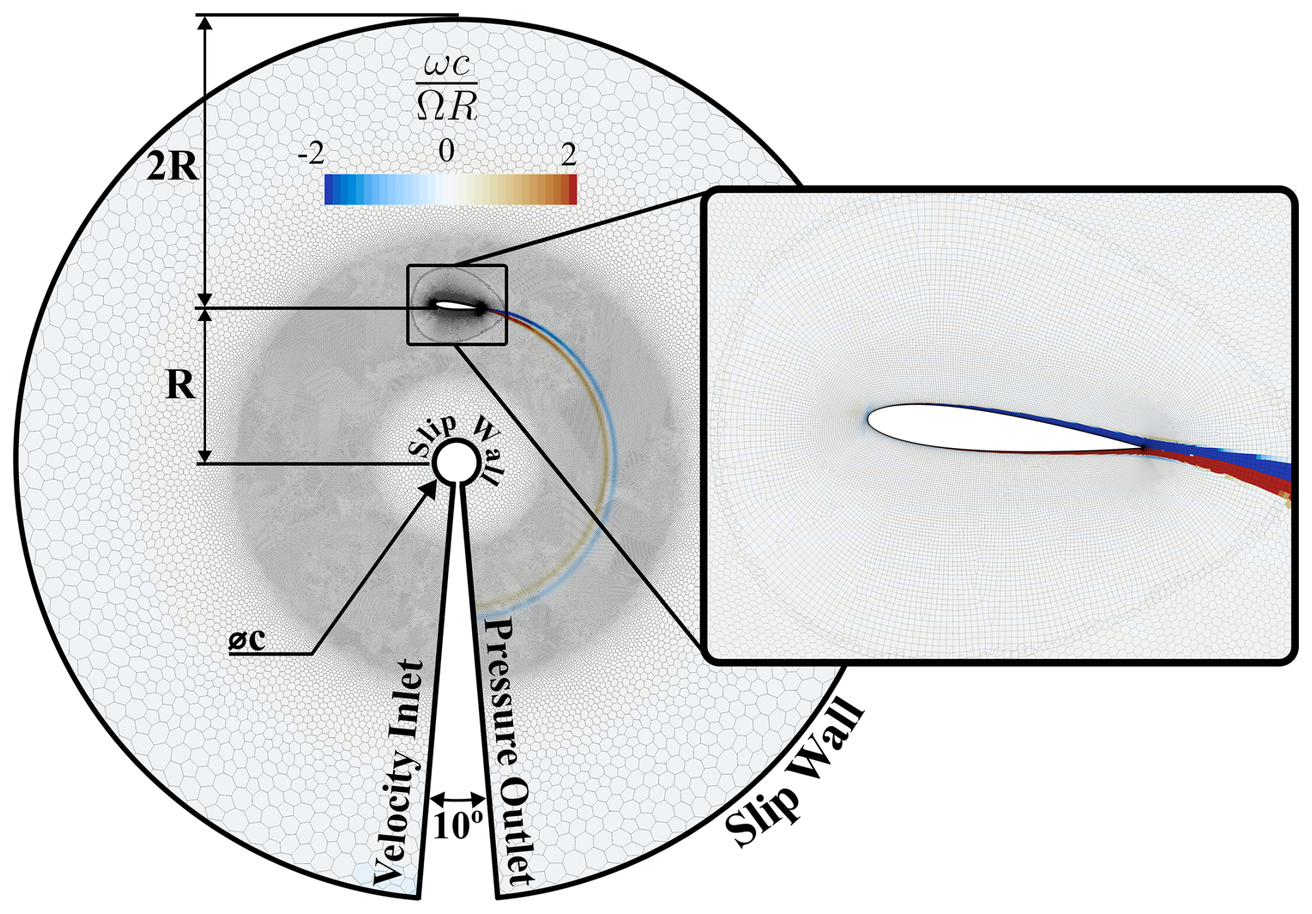
Figure B1 Simulation setup and key-hole mesh used for the simulation of the NACA0015 airfoil in rotation with $c/R=\mathrm{2}/\mathrm{7}$. Case with airfoil attached at mid-chord ($x_{\mathrm{p}}=c/\mathrm{2}$) and tilting angle α_p=6 °. A close-up of the body-fitted mesh around the airfoil is also shown.

B2 Airfoil attached at mid-chord ($x_{\mathrm{p}}=c/\mathrm{2}$)

The obtained aerodynamic coefficients are shown in Figs. B2–B4.

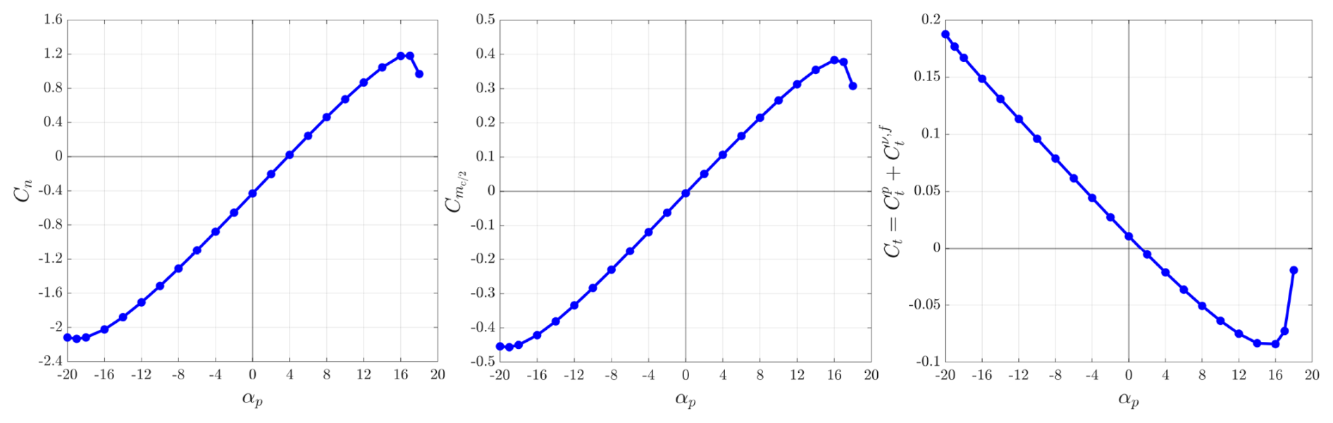
Figure B2 C_n, $C_{m_{c/\mathrm{2}}}$ and C_t as a function of the pitching angle α_p for the NACA0015 airfoil in rotation with $c/R=\mathrm{2}/\mathrm{7}$ and $x_{\mathrm{p}}=c/\mathrm{2}$.

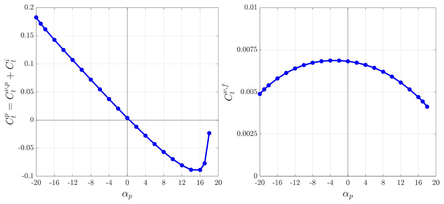
Figure B3 $C_{\mathrm{t}}^{\mathrm{p}}$ and $C_{\mathrm{t}}^{\mathit{\nu },\mathrm{f}}$ as a function of the pitching angle α_p for the NACA0015 airfoil in rotation with $c/R=\mathrm{2}/\mathrm{7}$ and $x_{\mathrm{p}}=c/\mathrm{2}$.

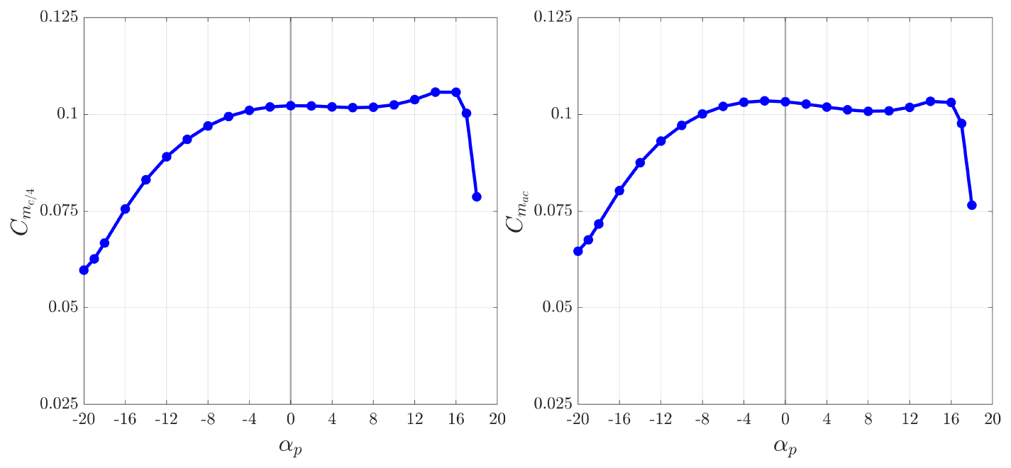
Figure B4 $C_{m_{c/\mathrm{4}}}$ and $C_{m_{\text{ac}}}$ as a function of the pitching angle α_p for the NACA0015 airfoil in rotation with $c/R=\mathrm{2}/\mathrm{7}$ and $x_{\mathrm{p}}=c/\mathrm{2}$.

B3 Airfoil attached at quarter-chord ($x_{\mathrm{p}}=c/\mathrm{4}$)

The obtained aerodynamic coefficients are shown in Figs. B5–B7.

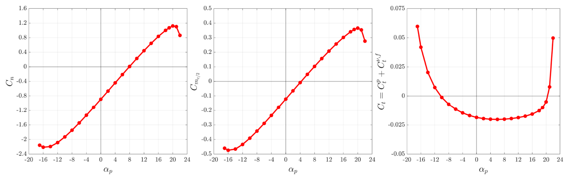
Figure B5 C_n, $C_{m_{c/\mathrm{2}}}$ and C_t as a function of the pitching angle α_p for the NACA0015 airfoil in rotation with $c/R=\mathrm{2}/\mathrm{7}$ and $x_{\mathrm{p}}=c/\mathrm{4}$.

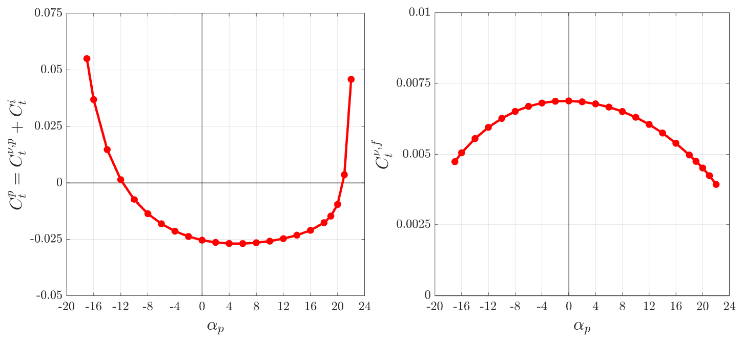
Figure B6 $C_{\mathrm{t}}^{\mathrm{p}}$ and $C_{\mathrm{t}}^{\mathit{\nu },\mathrm{f}}$ as a function of the pitching angle α_p for the NACA0015 airfoil in rotation with $c/R=\mathrm{2}/\mathrm{7}$ and $x_{\mathrm{p}}=c/\mathrm{4}$.

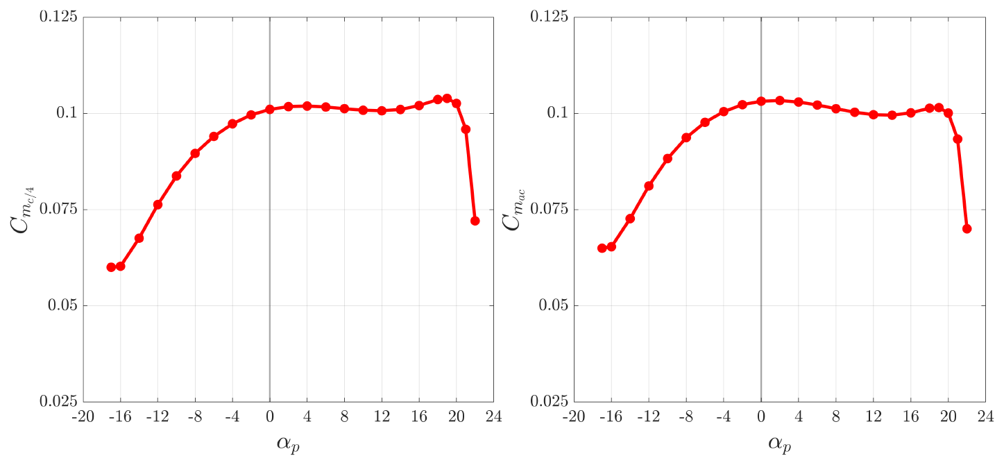
Figure B7 $C_{m_{c/\mathrm{4}}}$ and $C_{m_{\text{ac}}}$ as a function of the pitching angle α_p for the NACA0015 airfoil in rotation with $c/R=\mathrm{2}/\mathrm{7}$ and $x_{\mathrm{p}}=c/\mathrm{4}$.

B4 Comparison

The coefficients C_l, $C_{m_{c/\mathrm{2}}}$, C_d, $C_{\mathrm{d}}^{\mathrm{p}}$, $C_{\mathrm{d}}^{\mathit{\nu },f}$, $C_{m_{c/\mathrm{4}}}$ and $C_{m_{\text{ac}}}$ expressed as a function of the angle of attack α at $c/\mathrm{4}$ are compared in Figs. B8–B10. For the case where $x_{\mathrm{p}}=c/\mathrm{2}$, $\mathit{\alpha }={\mathit{\alpha }}_{\mathrm{p}}+{\mathit{\alpha }}_{\mathrm{c}}$, and for the case where $x_{\mathrm{p}}=c/\mathrm{4}$, α=α_p.

It is seen that the overlap is quite good. This supports the discussion made in the core of the paper that the “effective angle of attack” to consider in all cases is the angle that the airfoil chord makes relative to the streamline of the curved flow at the location of the aerodynamic center, in absence of the profile.

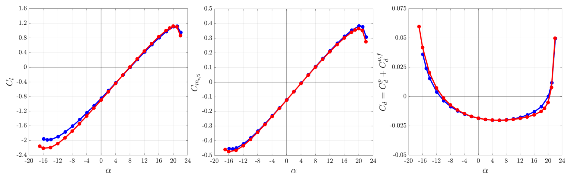
Figure B8 Comparison of the coefficients C_l, $C_{m_{c/\mathrm{2}}}$ and C_d as a function of the angle of attack α for the NACA0015 airfoil in rotation with $c/R=\mathrm{2}/\mathrm{7}$ and $x_{\mathrm{p}}=c/\mathrm{2}$ (blue) or $x_{\mathrm{p}}=c/\mathrm{4}$ (red).

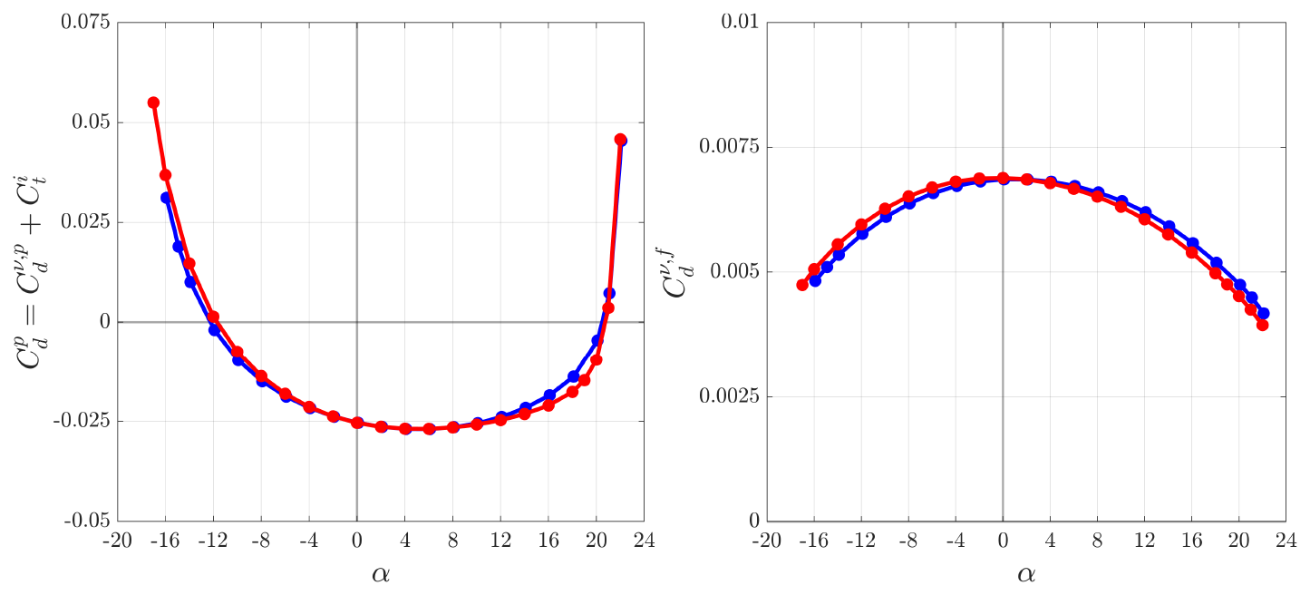
Figure B9 Comparison of the coefficients $C_{\mathrm{d}}^{\mathrm{p}}$ and $C_{\mathrm{d}}^{\mathit{\nu },\mathrm{f}}$ as a function of the angle of attack α for the NACA0015 airfoil in rotation with $c/R=\mathrm{2}/\mathrm{7}$ and $x_{\mathrm{p}}=c/\mathrm{2}$ (blue) or $x_{\mathrm{p}}=c/\mathrm{4}$ (red).

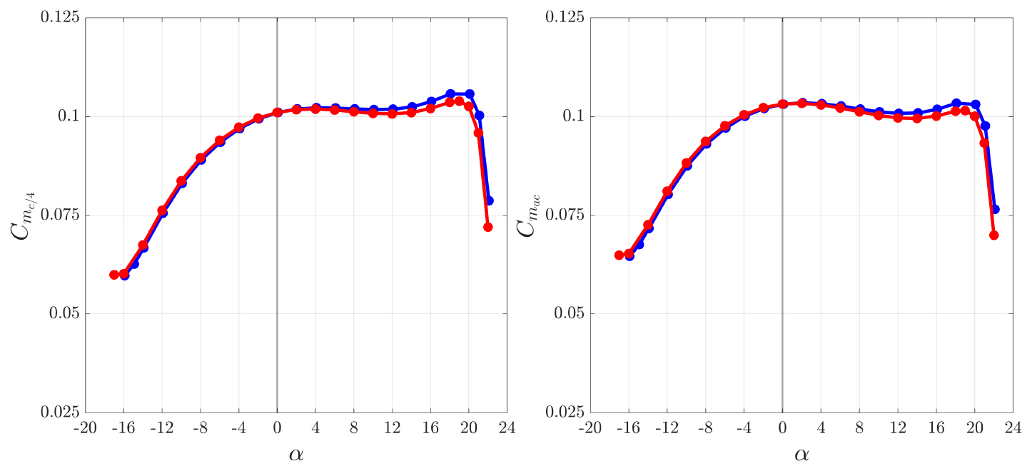
Figure B10 Comparison of the coefficients $C_{m_{c/\mathrm{4}}}$ and $C_{m_{\text{ac}}}$ as a function of the angle of attack α for the NACA0015 airfoil in rotation with $c/R=\mathrm{2}/\mathrm{7}$ and $x_{\mathrm{p}}=c/\mathrm{2}$ (blue) or $x_{\mathrm{p}}=c/\mathrm{4}$ (red).

Appendix C: Deformed NACA0015 airfoil in uniform flow and associated aerodynamic coefficients

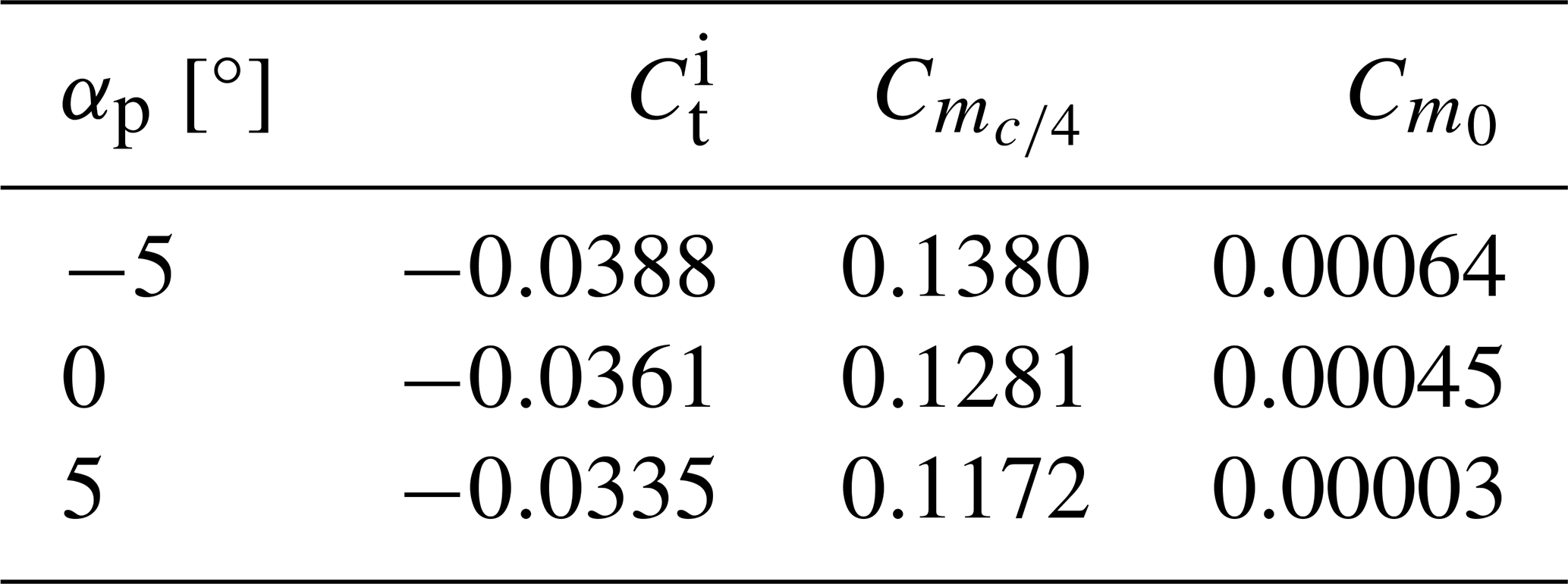
The flow past the NACA0015 airfoil deformed using the transformation $Z\left(z\right)=z+\frac{\mathrm{i}}{\mathrm{2}}\frac{z^{\mathrm{2}}}{R}$ was also obtained in uniform flow, using wall-resolved CFD at $R{e}_{\mathrm{c}}=\mathrm{6.0}\times {\mathrm{10}}^{\mathrm{6}}$. This allows one to measure the moment coefficient at mid-chord $C_{m_{c/\mathrm{2}}}^{\mathrm{0}}$ and then also account for it in the corrections for flow curvature effects. Table C1 provides the results for the deformed NACA0015 airfoil in uniform flow and the NACA0015 airfoil in curved flow, as well as an ALM simulation of the deformed NACA0015 airfoil in uniform flow with moment distribution.

As predicted using the analogy presented in Sect. 3, the coefficients of the deformed airfoil in uniform flow match those of the airfoil in curved flow. We also see that the ALM with distribution of the aerodynamic moment is able to successfully reproduce the results of the deformed airfoil in uniform flow. Figure C1 presents the vorticity field.

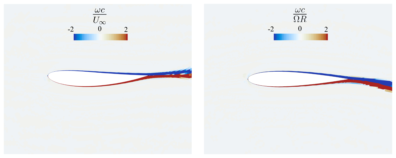
Figure C1 Vorticity field near the airfoil for the deformed airfoil in uniform flow (left) and the airfoil in curved flow (right).

Table C1 Coefficients for the deformed NACA0015 airfoil in uniform flow, the NACA0015 airfoil in curved flow and the ALM results of the deformed NACA0015 airfoil in uniform flow.

Appendix D: Inviscid flow simulations

The purpose of the inviscid flow simulations was to verify that the moment m₀ around the center of rotation of the arm is indeed zero when the flow is inviscid. We employ the same setup as that presented in Fig. B1. Additionally, a second-order implicit coupled flow solver is used to obtain the solution. The case studied is the NACA0015 airfoil attached at $x_{\mathrm{p}}=c/\mathrm{4}$. Each term of $C_{m_{\mathrm{0}}}\left({\mathit{\alpha }}_{\mathrm{p}}\right)=C_{m_{c/\mathrm{4}}}\left({\mathit{\alpha }}_{\mathrm{p}}\right)+\frac{R}{c}{C}_{\mathrm{t}}^{\mathrm{i}}\left({\mathit{\alpha }}_{\mathrm{p}}\right)$ is provided in Table D1. We see that $C_{m_{\mathrm{0}}}$ is indeed very close to zero; thereby confirming the argumentation that was used in developing the model for the inviscid contribution to the tangential force. Simulations were also attempted at higher pitch angles, but convergence became severely challenging due to the inviscid flow assumption.

Table D1 C_t, $C_{m_{c/\mathrm{4}}}$ and $C_{m_{\mathrm{0}}}$ as functions of the pitch angle α_p for the NACA0015 airfoil in inviscid curved flow with $c/R=\mathrm{2}/\mathrm{7}$. These values are obtained directly from the simulation, which explains why $C_{m_{c/\mathrm{4}}}\left({\mathit{\alpha }}_{\mathrm{p}}\right)+\frac{R}{c}{C}_{\mathrm{t}}\left({\mathit{\alpha }}_{\mathrm{p}}\right)$ does not exactly equal $C_{m_{\mathrm{0}}}$.

Appendix E: Solution of curved potential flow past a plate with pitch

We develop the exact solution for curved potential flow past a flat plate at various pitch angles. For this, we first consider the circle of radius a centered at the origin in a Z plane with (X,Y) coordinate system. We add a point vortex of circulation Γ₀<0 below the circle, at $Z_{\mathrm{0}}=-\mathrm{i}{R}_{\mathrm{0}}{\mathrm{e}}^{\mathrm{i}{\mathit{\alpha }}_{\mathrm{0}}}=R_{\mathrm{0}}\sin {\mathit{\alpha }}_{\mathrm{0}}-\mathrm{i}{R}_{\mathrm{0}}\cos {\mathit{\alpha }}_{\mathrm{0}}$. For the circle to be a streamline, we must add an image vortex of circulation $-{\mathrm{\Gamma }}_{\mathrm{0}}>\mathrm{0}$ inside the circle, at $Z_{\mathrm{1}}=-\mathrm{i}(a^{\mathrm{2}}/R_{\mathrm{0}}){\mathrm{e}}^{\mathrm{i}{\mathit{\alpha }}_{\mathrm{0}}}$. The complex potential is thus

$$\begin{array}{}\text{(E1)}& \begin{array}{rl}{\displaystyle }F\left(Z\right)=& {\displaystyle }\mathrm{\Phi }\left(Z\right)+\mathrm{i}\mathrm{\Psi }\left(Z\right)\\ {\displaystyle }=& {\displaystyle }-\mathrm{i}{\displaystyle \frac{{\mathrm{\Gamma }}_{\mathrm{0}}}{\mathrm{2}\mathit{\pi }}}\left[\log \left({\displaystyle \frac{Z-Z_{\mathrm{0}}}{a}}\right)-\log \left({\displaystyle \frac{Z-Z_{\mathrm{1}}}{a}}\right)\right]\\ {\displaystyle }=& {\displaystyle }-\mathrm{i}{\displaystyle \frac{{\mathrm{\Gamma }}_{\mathrm{0}}}{\mathrm{2}\mathit{\pi }}}\left[\log \left({\displaystyle \frac{Z+\mathrm{i}{R}_{\mathrm{0}}{\mathrm{e}}^{\mathrm{i}{\mathit{\alpha }}_{\mathrm{0}}}}{a}}\right)\right.\\ {\displaystyle }& {\displaystyle }\left.-\log \left({\displaystyle \frac{Z+\mathrm{i}(a^{\mathrm{2}}/R_{\mathrm{0}}){\mathrm{e}}^{\mathrm{i}{\mathit{\alpha }}_{\mathrm{0}}}}{a}}\right)\right],\end{array}\end{array}$$

with Φ the potential and Ψ the streamfunction. The velocity field is obtained as

$$\begin{array}{}\text{(E2)}& \begin{array}{rl}{\displaystyle \frac{\mathrm{d}F}{\mathrm{d}Z}}\left(Z\right)=& {\displaystyle }U\left(Z\right)-\mathrm{i}V\left(Z\right)\\ {\displaystyle }=& {\displaystyle }-\mathrm{i}{\displaystyle \frac{{\mathrm{\Gamma }}_{\mathrm{0}}}{\mathrm{2}\mathit{\pi }}}\left[{\displaystyle \frac{\mathrm{1}}{(Z-Z_{\mathrm{0}})}}-{\displaystyle \frac{\mathrm{1}}{(Z-Z_{\mathrm{1}})}}\right]\\ {\displaystyle }=& {\displaystyle }-{\displaystyle \frac{{\mathrm{\Gamma }}_{\mathrm{0}}}{\mathrm{2}\mathit{\pi }}}{\displaystyle \frac{\left(R_{\mathrm{0}}-a^{\mathrm{2}}/R_{\mathrm{0}}\right){\mathrm{e}}^{\mathrm{i}{\mathit{\alpha }}_{\mathrm{0}}}}{\left(Z^{\mathrm{2}}+\mathrm{i}\left(R_{\mathrm{0}}+a^{\mathrm{2}}/R_{\mathrm{0}}\right)Z{\mathrm{e}}^{\mathrm{i}{\mathit{\alpha }}_{\mathrm{0}}}-a^{\mathrm{2}}{\mathrm{e}}^{\mathrm{i}\mathrm{2}{\mathit{\alpha }}_{\mathrm{0}}}\right)}}.\end{array}\end{array}$$

The circle in the Z plane can be transformed into a horizontal flat plate in the z plane, with (x,y) coordinate system, using the conformal transformation:

$$\begin{array}{}\text{(E3)}& z\left(Z\right)=Z+{\displaystyle \frac{a^{\mathrm{2}}}{Z}}.\end{array}$$

The point $Z_L=-a$ is transformed into the plate leading edge $z_L=-\mathrm{2}a$, and the point Z_T=a is transformed into the plate trailing edge z_T=2 a. The chord of the plate is thus c=4 a. This transformation is also invertible, and we obtain

$$\begin{array}{}\text{(E4)}& Z\left(z\right)={\displaystyle \frac{\mathrm{1}}{\mathrm{2}}}\left(z+\sqrt{z^{\mathrm{2}}-\mathrm{4}{a}^{\mathrm{2}}}\right).\end{array}$$

The vortex located at $Z_{\mathrm{0}}=-\mathrm{i}{R}_{\mathrm{0}}{\mathrm{e}}^{\mathrm{i}{\mathit{\alpha }}_{\mathrm{0}}}$ in the Z plane in now located at $z_{\mathrm{0}}=Z_{\mathrm{0}}+a^{\mathrm{2}}/Z_{\mathrm{0}}=-\mathrm{i}R{\mathrm{e}}^{\mathrm{i}{\mathit{\alpha }}_{\mathrm{p}}}$ in the z plane, with

$$\begin{array}{}\text{(E5)}& \begin{array}{rl}{\displaystyle }& {\displaystyle }\left(R_{\mathrm{0}}+{\displaystyle \frac{a^{\mathrm{2}}}{R_{\mathrm{0}}}}\right)\sin {\mathit{\alpha }}_{\mathrm{0}}=R\sin {\mathit{\alpha }}_{\mathrm{p}}\text{and}\\ {\displaystyle }& {\displaystyle }\left(R_{\mathrm{0}}-{\displaystyle \frac{a^{\mathrm{2}}}{R_{\mathrm{0}}}}\right)\sin {\mathit{\alpha }}_{\mathrm{0}}=R\sin {\mathit{\alpha }}_{\mathrm{p}}.\end{array}\end{array}$$

To each choice of distance R and tilt angle α_p in the z plane, there is a corresponding distance R₀ and angle α₀ in the Z plane. For this, we write

$$\begin{array}{}\text{(E6)}& \begin{array}{rl}{\displaystyle }{z}_{\mathrm{0}}^{\mathrm{2}}-\mathrm{4}{a}^{\mathrm{2}}=& {\displaystyle }-\left(\left(R^{\mathrm{2}}\cos \left(\mathrm{2}{\mathit{\alpha }}_{\mathrm{p}}\right)+\mathrm{4}{a}^{\mathrm{2}}\right)+\mathrm{i}{R}^{\mathrm{2}}\sin \left(\mathrm{2}{\mathit{\alpha }}_{\mathrm{p}}\right)\right)\\ {\displaystyle }=& {\displaystyle }-{\stackrel{\mathrm{̃}}{R}}^{\mathrm{2}}{\mathrm{e}}^{\mathrm{i}\mathrm{2}\mathit{\beta }}.\end{array}\end{array}$$

The expressions for $\stackrel{\mathrm{̃}}{R}$ and β are obtained by identification:

$$\begin{array}{}\text{(E7)}& \begin{array}{rl}{\displaystyle }\stackrel{\mathrm{̃}}{R}=& {\displaystyle }{\left[{\left(R^{\mathrm{2}}\cos \left(\mathrm{2}{\mathit{\alpha }}_{\mathrm{p}}\right)+\mathrm{4}{a}^{\mathrm{2}}\right)}^{\mathrm{2}}+{\left(R^{\mathrm{2}}\sin \left(\mathrm{2}{\mathit{\alpha }}_{\mathrm{p}}\right)\right)}^{\mathrm{2}}\right]}^{\frac{\mathrm{1}}{\mathrm{4}}},\\ {\displaystyle }\mathit{\beta }=& {\displaystyle \frac{\mathrm{1}}{\mathrm{2}}}\arctan \left({\displaystyle \frac{R^{\mathrm{2}}\sin \left(\mathrm{2}{\mathit{\alpha }}_{\mathrm{p}}\right)}{R^{\mathrm{2}}\cos \left(\mathrm{2}{\mathit{\alpha }}_{\mathrm{p}}\right)+\mathrm{4}{a}^{\mathrm{2}}}}\right).\end{array}\end{array}$$

We hence finally obtain the position of Z₀

$$\begin{array}{}\text{(E8)}& Z_{\mathrm{0}}={\displaystyle \frac{\mathrm{1}}{\mathrm{2}}}\left(z_{\mathrm{0}}+\sqrt{z_{\mathrm{0}}^{\mathrm{2}}-\mathrm{4}{a}^{\mathrm{2}}}\right)=-{\displaystyle \frac{\mathrm{i}}{\mathrm{2}}}\left(R{\mathrm{e}}^{\mathrm{i}{\mathit{\alpha }}_{\mathrm{p}}}+\stackrel{\mathrm{̃}}{R}{\mathrm{e}}^{\mathrm{i}\mathit{\beta }}\right).\end{array}$$

Once Z₀ is known, its modulus R₀ and its angle α₀ can be easily calculated.

The baseline case α₀=0 is immediate as it corresponds to α_p=0, and thus also $R=R_{\mathrm{0}}\left(\mathrm{1}-\frac{a^{\mathrm{2}}}{R_{\mathrm{0}}^{\mathrm{2}}}\right)$. Inverting this relation gives

$$\begin{array}{}\text{(E9)}& \begin{array}{rl}{\displaystyle }{R}_{\mathrm{0}}=& {\displaystyle \frac{\mathrm{1}}{\mathrm{2}}}\left(R+\sqrt{R^{\mathrm{2}}-\mathrm{4}{a}^{\mathrm{2}}}\right)\\ {\displaystyle }=& {\displaystyle \frac{R}{\mathrm{2}}}\left(\mathrm{1}+\sqrt{\mathrm{1}+{\left({\displaystyle \frac{\mathrm{2}a}{R}}\right)}^{\mathrm{2}}}\right)\\ {\displaystyle }=& {\displaystyle \frac{R}{\mathrm{2}}}\left(\mathrm{1}+\sqrt{\mathrm{1}+{\left({\displaystyle \frac{c}{\mathrm{2}R}}\right)}^{\mathrm{2}}}\right).\end{array}\end{array}$$

We note that the obtained values of R₀ and α₀ are quite close to R and α_p when the vortex is far enough from the plate (i.e., when the ratio $c/R$ is “small enough”). For the case with significant curvature effects considered in this paper, this ratio is $c/R=\mathrm{2}/\mathrm{7}\simeq \mathrm{0.286}$. Clearly, this not very small; nevertheless, we obtain, for the case without tilt angle,

$$\begin{array}{}\text{(E10)}& {\displaystyle \frac{R_{\mathrm{0}}}{c}}\simeq \mathrm{3.518},\end{array}$$

which is still quite close to 3.50.

The complex potential of the flow past the plate in the z plane is

$$\begin{array}{}\text{(E11)}& f\left(z\right)=\mathit{\varphi }\left(z\right)+\mathrm{i}\mathit{\psi }\left(z\right),\end{array}$$

and it is obtained by writing f(z)=F(Z) for z=z(Z). The velocity field is then obtained using

$$\begin{array}{}\text{(E12)}& {\displaystyle \frac{\mathrm{d}f}{\mathrm{d}z}}\left(z\right)=u\left(z\right)-\mathrm{i}v\left(z\right)={\displaystyle \frac{\frac{\mathrm{d}F}{\mathrm{d}Z}\left(Z\right)}{\frac{\mathrm{d}z}{\mathrm{d}Z}\left(Z\right)}}\text{for }z=z\left(Z\right).\end{array}$$

To enforce the condition that the flow leaves the plate smoothly at its trailing edge, with a finite velocity there (i.e., the “Kutta–Joukowski condition”), we must add another vortex of circulation Γ_c at the center of the circle, the circulation of which being computed so that $\frac{\mathrm{d}f}{\mathrm{d}z}\left(z_{\mathrm{T}}\right)$ is finite. As $\frac{\mathrm{d}z}{\mathrm{d}Z}(Z_{\mathrm{T}}=a)=\mathrm{0}$ (since Z_T=a is a singular point of the transformation z(Z)), we must impose that $\frac{\mathrm{d}F}{\mathrm{d}Z}(Z_{\mathrm{T}}=a)=\mathrm{0}$. The complex potential with the added vortex is, hence,

$$\begin{array}{}\text{(E13)}& \begin{array}{rl}{\displaystyle }F\left(Z\right)=& {\displaystyle }-\mathrm{i}{\displaystyle \frac{{\mathrm{\Gamma }}_{\mathrm{0}}}{\mathrm{2}\mathit{\pi }}}\left[\log \left({\displaystyle \frac{Z-Z_{\mathrm{0}}}{a}}\right)-\log \left({\displaystyle \frac{Z-Z_{\mathrm{1}}}{a}}\right)\right.\\ {\displaystyle }& {\displaystyle }\left.+{\displaystyle \frac{{\mathrm{\Gamma }}_{\mathrm{c}}}{{\mathrm{\Gamma }}_{\mathrm{0}}}}\log \left({\displaystyle \frac{Z}{a}}\right)\right],\end{array}\end{array}$$

and thus

$$\begin{array}{}\text{(E14)}& \begin{array}{rl}{\displaystyle }& {\displaystyle \frac{\mathrm{d}F}{\mathrm{d}Z}}\left(Z\right)\\ {\displaystyle }& {\displaystyle }=-\mathrm{i}{\displaystyle \frac{{\mathrm{\Gamma }}_{\mathrm{0}}}{\mathrm{2}\mathit{\pi }}}\left[{\displaystyle \frac{\mathrm{1}}{(Z-Z_{\mathrm{0}})}}-{\displaystyle \frac{\mathrm{1}}{(Z-Z_{\mathrm{1}})}}+{\displaystyle \frac{{\mathrm{\Gamma }}_{\mathrm{c}}}{{\mathrm{\Gamma }}_{\mathrm{0}}}}{\displaystyle \frac{\mathrm{1}}{Z}}\right]\\ {\displaystyle }& {\displaystyle }=-\mathrm{i}{\displaystyle \frac{{\mathrm{\Gamma }}_{\mathrm{0}}}{\mathrm{2}\mathit{\pi }}}\left[{\displaystyle \frac{\mathrm{i}\left(a^{\mathrm{2}}/R_{\mathrm{0}}-R_{\mathrm{0}}\right){\mathrm{e}}^{\mathrm{i}{\mathit{\alpha }}_{\mathrm{0}}}}{\left(Z^{\mathrm{2}}+\mathrm{i}\left(R_{\mathrm{0}}+a^{\mathrm{2}}/R_{\mathrm{0}}\right){\mathrm{e}}^{\mathrm{i}{\mathit{\alpha }}_{\mathrm{0}}}Z-a^{\mathrm{2}}{\mathrm{e}}^{\mathrm{i}\mathrm{2}{\mathit{\alpha }}_{\mathrm{0}}}\right)}}+{\displaystyle \frac{{\mathrm{\Gamma }}_{\mathrm{c}}}{{\mathrm{\Gamma }}_{\mathrm{0}}}}{\displaystyle \frac{\mathrm{1}}{Z}}\right].\end{array}\end{array}$$

Imposing $\frac{\mathrm{d}F}{\mathrm{d}Z}\left(a\right)=\mathrm{0}$ determines the circulation of the added vortex:

$$\begin{array}{}\text{(E15)}& {\mathrm{\Gamma }}_{\mathrm{c}}={\displaystyle \frac{\left(R_{\mathrm{0}}-a^{\mathrm{2}}/R_{\mathrm{0}}\right)}{\left(\left(R_{\mathrm{0}}+a^{\mathrm{2}}/R_{\mathrm{0}}\right)-\mathrm{2}a\sin {\mathit{\alpha }}_{\mathrm{0}}\right)}}{\mathrm{\Gamma }}_{\mathrm{0}}.\end{array}$$

The total circulation of the flow around the plate in the z plane (and also around the circle in the Z plane) is the sum of the circulations of the two vortices inside the circle:

$$\begin{array}{}\text{(E16)}& \begin{array}{rl}{\displaystyle }\mathrm{\Gamma }=& {\displaystyle }{\mathrm{\Gamma }}_{\mathrm{c}}+(-{\mathrm{\Gamma }}_{\mathrm{0}})\\ {\displaystyle }=& {\displaystyle }-\mathrm{2}{\displaystyle \frac{\left(a^{\mathrm{2}}/R_{\mathrm{0}}+a\sin {\mathit{\alpha }}_{\mathrm{0}}\right)}{\left(\left(R_{\mathrm{0}}+a^{\mathrm{2}}/R_{\mathrm{0}}\right)-\mathrm{2}a\sin {\mathit{\alpha }}_{\mathrm{0}}\right)}}{\mathrm{\Gamma }}_{\mathrm{0}}.\end{array}\end{array}$$

For the case α₀=0, we obtain

$$\begin{array}{}\text{(E17)}& \mathrm{\Gamma }=-\mathrm{2}{\displaystyle \frac{\frac{a^{\mathrm{2}}}{R_{\mathrm{0}}^{\mathrm{2}}}}{\left(\mathrm{1}+\frac{a^{\mathrm{2}}}{R_{\mathrm{0}}^{\mathrm{2}}}\right)}}{\mathrm{\Gamma }}_{\mathrm{0}}>\mathrm{0}.\end{array}$$

We also note that the circulation Γ is zero when $\sin \left({\mathit{\alpha }}_{\mathrm{0}}\right)=-a/R_{\mathrm{0}}$; this corresponds to the case without force exerted by the flow on the plate.

Finally, the forces exerted by the flow on the plate can be obtained using Blasius formula:

$$\begin{array}{}\text{(E18)}& \begin{array}{rl}{\displaystyle }{f}_x-\mathrm{i}{f}_y=& {\displaystyle }\mathrm{i}{\displaystyle \frac{\mathit{\rho }}{\mathrm{2}}}\underset{C_z}{\oint }{\left({\displaystyle \frac{\mathrm{d}f}{\mathrm{d}z}}\left(z\right)\right)}^{\mathrm{2}}\mathrm{d}z\\ {\displaystyle }=& {\displaystyle }\mathrm{i}{\displaystyle \frac{\mathit{\rho }}{\mathrm{2}}}\underset{C_Z}{\oint }{\displaystyle \frac{{\left(\frac{\mathrm{d}F}{\mathrm{d}Z}\left(Z\right)\right)}^{\mathrm{2}}}{\frac{\mathrm{d}z}{\mathrm{d}Z}\left(Z\right)}}\mathrm{d}Z.\end{array}\end{array}$$

We have used the change in variable, z(Z), as the integral must be performed in the Z plane using a contour C_Z that contains the circle but excludes the outer vortex. Since $\frac{\mathrm{d}z}{\mathrm{d}Z}\left(Z\right)=\frac{(Z^{\mathrm{2}}-a^{\mathrm{2}})}{Z^{\mathrm{2}}}$, we obtain

$$\begin{array}{}\text{(E19)}& \begin{array}{rl}{\displaystyle }{f}_x-\mathrm{i}{f}_y=& {\displaystyle }-\mathrm{i}{\displaystyle \frac{\mathit{\rho }}{\mathrm{2}}}{\left({\displaystyle \frac{{\mathrm{\Gamma }}_{\mathrm{0}}}{\mathrm{2}\mathit{\pi }}}\right)}^{\mathrm{2}}\underset{C_Z}{\oint }\left[{\displaystyle \frac{\mathrm{1}}{(Z-Z_{\mathrm{0}})}}-{\displaystyle \frac{\mathrm{1}}{(Z-Z_{\mathrm{1}})}}\right.\\ {\displaystyle }& {\displaystyle }{\left.+{\displaystyle \frac{{\mathrm{\Gamma }}_{\mathrm{c}}}{{\mathrm{\Gamma }}_{\mathrm{0}}}}{\displaystyle \frac{\mathrm{1}}{Z}}\right]}^{\mathrm{2}}{\displaystyle \frac{Z^{\mathrm{2}}}{(Z^{\mathrm{2}}-a^{\mathrm{2}})}}\mathrm{d}Z\\ {\displaystyle }=& {\displaystyle }-\mathrm{i}{\displaystyle \frac{\mathit{\rho }}{\mathrm{2}}}{\left({\displaystyle \frac{{\mathrm{\Gamma }}_{\mathrm{0}}}{\mathrm{2}\mathit{\pi }}}\right)}^{\mathrm{2}}\underset{C_Z}{\oint }G\left(Z\right)\mathrm{d}Z.\end{array}\end{array}$$

The contour integral must be performed using the residue theorem:

$$\begin{array}{}\text{(E20)}& \begin{array}{rl}{\displaystyle }& {\displaystyle }\underset{C_Z}{\oint }G\left(Z\right)\mathrm{d}Z=\\ {\displaystyle }& {\displaystyle }\mathrm{2}\mathit{\pi }i\sum \text{residues of }G\left(Z\right)\text{ inside }{C}_Z.\end{array}\end{array}$$

We thus finally obtain

$$\begin{array}{}\text{(E21)}& f_x-\mathrm{i}{f}_y=\mathit{\rho }{\displaystyle \frac{{\mathrm{\Gamma }}_{\mathrm{0}}^{\mathrm{2}}}{\mathrm{4}\mathit{\pi }}}\sum \text{residues of }G\left(Z\right)\text{ inside }{C}_Z.\end{array}$$

It turns out that the only non-zero residues of G(Z) are those evaluated at $Z_{\mathrm{1}}=-\mathrm{i}(a^{\mathrm{2}}/R_{\mathrm{0}}){\mathrm{e}}^{\mathrm{i}{\mathit{\alpha }}_{\mathrm{0}}}$.

For the case α₀=0 with the vortex just below the plate, and thus α_p=0, the flow past the plate is left/right symmetric; hence f_x(0)=0 and f_y(0) is also the force normal to the plate, f_n(0). The sum of the residues is then obtained as

$$\begin{array}{}\text{(E22)}& \mathrm{i}{\displaystyle \frac{\mathrm{1}}{R_{\mathrm{0}}\left(\mathrm{1}-\frac{a^{\mathrm{2}}}{R_{\mathrm{0}}^{\mathrm{2}}}\right)}}{\displaystyle \frac{\mathrm{4}\frac{a^{\mathrm{2}}}{R_{\mathrm{0}}^{\mathrm{2}}}}{{\left(\mathrm{1}+\frac{a^{\mathrm{2}}}{R_{\mathrm{0}}^{\mathrm{2}}}\right)}^{\mathrm{2}}}},\end{array}$$

and we finally obtain

$$\begin{array}{}\text{(E23)}& \begin{array}{rl}{\displaystyle }{f}_y\left(\mathrm{0}\right)=& {\displaystyle }{f}_{\mathrm{n}}\left(\mathrm{0}\right)=-\mathit{\rho }{\displaystyle \frac{{\mathrm{\Gamma }}_{\mathrm{0}}}{\mathrm{2}\mathit{\pi }{R}_{\mathrm{0}}\left(\mathrm{1}-\frac{a^{\mathrm{2}}}{R_{\mathrm{0}}^{\mathrm{2}}}\right)}}{\displaystyle \frac{\mathrm{2}\frac{a^{\mathrm{2}}}{R_{\mathrm{0}}^{\mathrm{2}}}}{{\left(\mathrm{1}+\frac{a^{\mathrm{2}}}{R_{\mathrm{0}}^{\mathrm{2}}}\right)}^{\mathrm{2}}}}{\mathrm{\Gamma }}_{\mathrm{0}}\\ {\displaystyle }=& {\displaystyle }\mathit{\rho }{\displaystyle \frac{{\mathrm{\Gamma }}_{\mathrm{0}}}{\mathrm{2}\mathit{\pi }R}}{\displaystyle \frac{\mathrm{\Gamma }}{\left(\mathrm{1}+\frac{a^{\mathrm{2}}}{R_{\mathrm{0}}^{\mathrm{2}}}\right)}}=-\mathit{\rho }U{\displaystyle \frac{\mathrm{\Gamma }}{\left(\mathrm{1}+\frac{a^{\mathrm{2}}}{R_{\mathrm{0}}^{\mathrm{2}}}\right)}}<\mathrm{0},\end{array}\end{array}$$

where we recalled the horizontal velocity $U=-\frac{{\mathrm{\Gamma }}_{\mathrm{0}}}{\mathrm{2}\mathit{\pi }R}>\mathrm{0}$ induced by the vortex and evaluated at the plate center. The lift of the curved flow past the plate with the vortex directly below it is thus almost equal to −ρ U Γ: the usual formula for a plate or airfoil in a free stream at velocity U, with circulation Γ of the flow around it and without anything else nearby.

Using Eq. (E9), we obtain

$$\begin{array}{}\text{(E24)}& {\displaystyle \frac{a}{R_{\mathrm{0}}}}={\displaystyle \frac{\frac{c}{\mathrm{2}R}}{\left(\mathrm{1}+\sqrt{\mathrm{1}+{\left(\frac{c}{\mathrm{2}R}\right)}^{\mathrm{2}}}\right)}},\end{array}$$

and the normal force coefficient is finally obtained as

$$\begin{array}{}\text{(E25)}& \begin{array}{rl}{\displaystyle }{C}_{\mathrm{n}}\left(\mathrm{0}\right)=& {\displaystyle \frac{f_{\mathrm{n}}}{\frac{\mathrm{1}}{\mathrm{2}}\mathit{\rho }{U}^{\mathrm{2}}c}}=-\mathit{\pi }{\displaystyle \frac{\frac{c}{\mathrm{2}R}}{\left(\mathrm{1}+{\left(\frac{c}{\mathrm{2}R}\right)}^{\mathrm{2}}\right)}}\\ {\displaystyle }=& {\displaystyle }-{\displaystyle \frac{\mathrm{2}\mathit{\pi }}{\left(\mathrm{1}+{\left(\frac{c}{\mathrm{2}R}\right)}^{\mathrm{2}}\right)}}{\displaystyle \frac{c}{\mathrm{4}R}}.\end{array}\end{array}$$

Consider the straight line that goes from the vortex to the plate leading (or trailing) edge: it makes an angle ϕ_c with the line that goes from the vortex to the center of the plate, such that $\tan \left({\mathit{\varphi }}_{\mathrm{c}}\right)=\frac{c}{\mathrm{2}R}$. We thus obtain

$$\begin{array}{}\text{(E26)}& \begin{array}{rl}{\displaystyle \frac{\frac{c}{\mathrm{2}R}}{\left(\mathrm{1}+{\left(\frac{c}{\mathrm{2}R}\right)}^{\mathrm{2}}\right)}}=& {\displaystyle \frac{\tan \left(\mathit{\varphi }\right)}{\left(\mathrm{1}+{\tan }^{\mathrm{2}}\left({\mathit{\varphi }}_{\mathrm{c}}\right)\right)}}\\ {\displaystyle }=& {\displaystyle \frac{\mathrm{1}}{\mathrm{2}}}\sin \left({\mathit{\varphi }}_{\mathrm{c}}\right)\cos \left({\mathit{\varphi }}_{\mathrm{c}}\right)={\displaystyle \frac{\mathrm{1}}{\mathrm{4}}}\sin \left(\mathrm{2}{\mathit{\varphi }}_{\mathrm{c}}\right),\end{array}\end{array}$$

and hence

$$\begin{array}{}\text{(E27)}& C_{\mathrm{n}}\left(\mathrm{0}\right)=-\mathrm{2}\mathit{\pi }{\displaystyle \frac{\sin \left(\mathrm{2}{\mathit{\varphi }}_{\mathrm{c}}\right)}{\mathrm{4}}}.\end{array}$$

We also define the half angle (used in the curvature correction models), ${\mathit{\alpha }}_{\mathrm{c}}={\mathit{\varphi }}_{\mathrm{c}}/\mathrm{2}$, and write this as

$$\begin{array}{}\text{(E28)}& C_{\mathrm{n}}\left(\mathrm{0}\right)=-\mathrm{2}\mathit{\pi }{\displaystyle \frac{\sin \left(\mathrm{4}{\mathit{\alpha }}_{\mathrm{c}}\right)}{\mathrm{4}}}.\end{array}$$

We have

$$\begin{array}{}\text{(E29)}& {\displaystyle \frac{c}{\mathrm{2}R}}=\tan \left({\mathit{\varphi }}_{\mathrm{c}}\right)=\tan \left(\mathrm{2}{\mathit{\alpha }}_{\mathrm{c}}\right)={\displaystyle \frac{\mathrm{2}\tan \left({\mathit{\alpha }}_{\mathrm{c}}\right)}{\left(\mathrm{1}-{\tan }^{\mathrm{2}}\left({\mathit{\alpha }}_{\mathrm{c}}\right)\right)}},\end{array}$$

which constitutes a quadratic equation for tan (α_c). The solution is

$$\begin{array}{}\text{(E30)}& \tan \left({\mathit{\alpha }}_{\mathrm{c}}\right)={\displaystyle \frac{\left(\sqrt{\mathrm{1}+{\left(\frac{c}{\mathrm{2}R}\right)}^{\mathrm{2}}}-\mathrm{1}\right)}{\frac{c}{\mathrm{2}R}}}.\end{array}$$

The streamlines of the flows obtained are shown in Fig. 1 for the case $c/R=\mathrm{2}/\mathrm{7}$ and for different values of the tilt angle α_p of the plate relative to the vortex. To clearly show the flow relative to the plate, we present the streamlines in the coordinate system used in the core of the paper: the vortex Γ₀ is located at $(\mathrm{0},-R)$ below the plate and the plate is tilted by an angle α_p relative to the horizontal. For the case with α_p=0, the flow is left/right symmetric. For the case with ${\mathit{\alpha }}_{\mathrm{p}}=-\mathrm{4}\mathit{°}$, the force exerted by the flow is close to zero (it is exactly zero when α_p≃4.185 °).

All the results obtained above are exact within the framework of potential flow theory. Now, for cases with ${\left(\frac{c}{\mathrm{2}R}\right)}^{\mathrm{2}}\ll \mathrm{1}$, as with those considered in this paper, we can simply write

$$\begin{array}{}\text{(E31)}& \begin{array}{rl}{\displaystyle }& {\displaystyle }{C}_{\mathrm{n}}\left(\mathrm{0}\right)\simeq -\mathrm{2}\mathit{\pi }\sin \left({\mathit{\alpha }}_{\mathrm{c}}\right)\text{with}\\ {\displaystyle }& {\displaystyle }\sin \left({\mathit{\alpha }}_{\mathrm{c}}\right)\simeq {\mathit{\alpha }}_{\mathrm{c}}\simeq {\displaystyle \frac{{\mathit{\varphi }}_{\mathrm{c}}}{\mathrm{2}}}\simeq {\displaystyle \frac{\mathrm{1}}{\mathrm{2}}}\left({\displaystyle \frac{c}{\mathrm{2}R}}\right).\end{array}\end{array}$$