A wind turbine digital shadow for complex inflow conditions

We present a digital shadow Kalman filtering framework based on the direct linearization of a trusted multibody aeroservoelastic wind turbine model. In contrast to shadowing based on ad hoc modeling approaches, reusing validated industrial or research-grade models reduces the development effort, leverages resources invested in tuning and validation, and, eventually, increases confidence in the results.

Building on earlier work, the filter-internal model is extended to improve applicability under non-symmetric, waked, and yaw-misaligned inflow conditions. In addition to tower fore–aft and rotor-speed dynamics, the model incorporates tower side–side motion as well as blade flapwise and edgewise degrees of freedom. Real-time inflow observers estimate rotor-equivalent wind speed, vertical and horizontal shear, and yaw misalignment, enabling operating-point-dependent scheduling of the linearized model. To further enhance predictive accuracy, the white-box model is augmented with data-driven corrections, considering both a bias-correction approach that acts on states and outputs, and a neural-network-based output correction.

The proposed method is validated in simulation under freestream, waked, and wake-steering scenarios and subsequently on field data from an instrumented wind turbine. Additional field cases with extreme shear and waked operation are used to assess robustness. Even without data-driven correction, damage-equivalent loads estimated from field data exhibit accuracy comparable to simulation-based results. When correction strategies are applied, accuracy improves substantially, with damage-equivalent load errors reduced to only a few percent.

1 Introduction

Digital twins for wind turbine applications have recently garnered significant attention, emerging as key components of modern wind systems. They support control (Anand and Bottasso, 2023), lifetime estimation (Branlard et al., 2020b; Song et al., 2023), and asset monitoring (Olatunji et al., 2021). Because wind turbines operate autonomously in complex and variable conditions, the ability to mirror the behavior of each asset offers substantial potential. Combined with machine learning and artificial intelligence, digital representations can continually improve, thereby enhancing productivity and profitability.

Digital twins build on the predictive abilities of digital shadows, which rely on a one-way data flow from the physical asset to the model, unlike twins, where the loop is closed (Sepasgozar, 2021). As this work focuses solely on accurate mirroring, we adopt the term digital shadow (Hoghooghi et al., 2024).

Among the many possible formulations, we follow and extend an approach that integrates an aeroservoelastic model with a Kalman filter (Grewal and Andrews, 2014; Branlard, 2019; Branlard et al., 2024a; Hoghooghi et al., 2024). Wind turbine manufacturers already maintain trusted and validated aeroservoelastic models, which are ideal candidates for the development of digital shadows. Using these models eliminates the need to rebuild ad hoc representations and provides immediate predictive capabilities, even without extensive field datasets – an advantage over purely data-driven approaches that require lengthy and expensive measurement campaigns. Moreover, a white-box model can later be augmented with data-driven corrections, evolving into an adaptive gray model.

Following Branlard (2019) and Branlard et al. (2024a), an aeroservoelastic model is linearized around multiple operating conditions, yielding a linear state-space internal model updated at each time step via SCADA measurements. Here, we improve this framework in four main ways.

First, the internal model is expanded beyond tower fore–aft and rotor-speed dynamics to include tower side–side motion and blade flapwise and edgewise degrees of freedom (DOFs). This richer representation extends applicability to strongly sheared, waked, and yaw-misaligned conditions relevant to wake-steering control.

Second, the wider operating envelope requires more advanced scheduling. Accordingly, the model is scheduled not only by wind speed but also by vertical shear, horizontal shear (capturing wake impingement), and yaw misalignment. These inflow parameters are estimated in real time using dedicated observers (Kim et al., 2023; Bertelè et al., 2024).

Third, a bias-correction procedure improves the accuracy of both state and output equations. State biases are compensated through additive error terms in the dynamic equilibrium, calibrated as a function of the current operating state. Output biases are promoted to state variables governed by process noise. Although more general nonlinear corrections (Bottasso et al., 2006) are possible, the adopted approach already delivers substantial improvements in fatigue-damage estimation.

Fourth, for condition monitoring applications, the model is enhanced via a data-driven learning element that corrects selected outputs using measurements from onboard sensors. A neural-based term is trained on the observed discrepancies and added to the corresponding model equations, yielding highly accurate predictions suitable for anomaly detection.

The digital shadow is demonstrated in simulation under clean freestream, waked, and wake-steering conditions, and validated with field data from an instrumented multi-MW turbine under both clean and complex inflow. The implementation utilizes OpenFAST and its associated tools (OpenFAST, 2024; Jonkman and Shaler, 2021; TurbSim, 2023), with the filter realized in MATLAB (The MathWorks, Inc., 2022), although the methodology is general and software independent.

Fatigue-related applications of digital twins are extensively documented (Bernhammer et al., 2016; Hoghooghi et al., 2019a, b), as fatigue loads affect all major components (IEC, 2019; Hoghooghi, 2021) and directly influence lifetime, performance, and cost (Bottasso et al., 2013; Loew and Bottasso, 2022; Dimitrov et al., 2018). Condition monitoring (CM) supports proactive maintenance and improved operational efficiency (Chen et al., 2016; Wu et al., 2021; Liu et al., 2023), with several methods leveraging machine learning (Bangalore et al., 2017; Hoghooghi et al., 2020a, b, 2021; Surucu et al., 2023). Numerous load-estimation techniques also exist, ranging from hybrid physics-data methods (Noppe et al., 2016) to lookup tables (Mendez Reyes et al., 2019), modal expansion (Iliopoulos et al., 2016), ensemble-based fatigue aggregation (Abdallah et al., 2017), machine learning (Evans et al., 2018), neural networks (Schröder et al., 2018), polynomial chaos (Dimitrov et al., 2018), deconvolution (Jacquelin et al., 2003), load extrapolation (Ziegler et al., 2017), virtual sensing via ROM–FE coupling (Vettori et al., 2022), and NN-based surrogates (Guilloré et al., 2024).

This brief overview illustrates the broad relevance of digital shadows for turbine health monitoring and fatigue estimation. The present work contributes by formulating a general procedure for digital shadow development that leverages trusted multibody models, linearization for computational efficiency, and adaptive corrections informed by inflow estimators and learning elements for improved accuracy.

The paper is organized as follows. Section 2 describes the methodology, including the internal model, its scheduling, and correction strategies. Section 3 evaluates performance in simulation and field conditions. Section 4 summarizes findings and outlines future work.

2 Methods

Figure 1 illustrates the main components of the proposed digital shadow workflow. A Kalman filter combines SCADA measurements with the predictions of a turbine ROM to estimate system states and additional outputs. The filter-internal model is obtained by linearizing a higher-fidelity multibody model of the turbine. Blade-load measurements are combined with SCADA data to infer key inflow characteristics in real time. These inflow parameters are then used to schedule the coefficients of the filter-internal model, enabling the filter to adapt to the full range of operating and inflow conditions experienced by the turbine.

Figure 1 Schematic representation of the proposed digital shadowing approach.

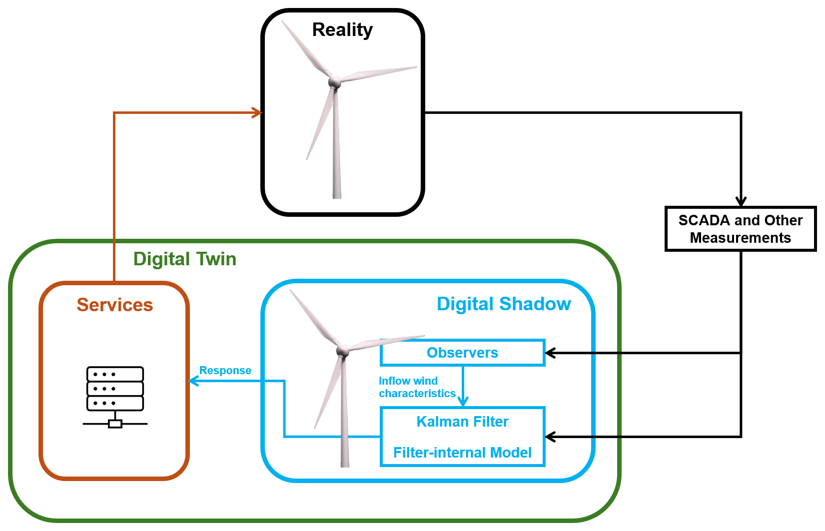
The proposed digital shadow combines a physics-based reduced-order model with real-time measurements to continuously estimate the turbine dynamic state and selected unmeasured loads. The Kalman filter serves as the core data-fusion mechanism, propagating the turbine response using the linearized aeroelastic model and correcting these predictions whenever new measurements become available. Model scheduling ensures that the filter remains valid across varying inflow and operating conditions by adjusting the model coefficients in real time.

2.1 Filter-internal model

We consider a nonlinear multibody model of a wind turbine, expressed in terms of generalized displacements q, velocities v, and inputs u. Noisy measurements ν affect the outputs y used by the filter to update the model states, while z denotes additional outputs of interest that do not participate in the innovation step. The filter ROM is obtained by directly linearizing the nonlinear model around multiple equilibrium conditions, with equilibrium vectors q₀, v₀, u₀, y₀, and z₀. The resulting filter-internal linear model is formulated in terms of increments δ(⋅) as

$$\begin{array}{}\text{(1a)}& {\displaystyle }\dot{\mathit{\delta }\mathit{q}}=\mathit{\delta }\mathit{v},\text{(1b)}& {\displaystyle }\dot{\mathit{\delta }\mathit{v}}=-{\mathbf{M}}^{-\mathrm{1}}(\mathbf{C}\mathit{\delta }\mathit{v}+\mathbf{K}\mathit{\delta }\mathit{q}+\mathbf{U}\mathit{\delta }\mathit{u}+\mathit{\omega }),\text{(1c)}& {\displaystyle }\mathit{\delta }\mathit{y}={\mathbf{D}}_v\mathit{\delta }\mathit{v}+{\mathbf{D}}_q\mathit{\delta }\mathit{q}+\mathbf{E}\mathit{\delta }\mathit{u}+\mathit{\nu },\text{(1d)}& {\displaystyle }\mathit{\delta }\mathit{z}={\mathbf{F}}_v\mathit{\delta }\mathit{v}+{\mathbf{F}}_q\mathit{\delta }\mathit{q}+\mathbf{G}\mathit{\delta }\mathit{u}.\end{array}$$

The Kalman filter integrates the linearized model by first predicting the system states and their uncertainties, and then correcting these predictions using the available measurements and their associated noise characteristics. Because the underlying model is linearized, the nonlinear values of all quantities are recovered by adding the perturbations to the corresponding equilibrium values, e.g. $\mathit{q}={\mathit{q}}_{\mathrm{0}}+\mathit{\delta }\mathit{q}$, and analogously for all other vectors in Eq. (1).

Equation (1a) represents the (noise-free) kinematic relations, while Eq. (1b) expresses the dynamic equilibrium affected by process noise ω, with M, C, K, and U denoting the mass, damping, stiffness, and control matrices, respectively. Equations (1c) and (1d) give the linearized output relations for y and z, respectively. All noise terms are assumed to be zero-mean and uncorrelated (Grewal and Andrews, 2014).

Although a standard linear Kalman filter would be sufficient for the present linearized state-space model, we adopt the unscented Kalman filter (UKF) implementation of MATLAB (Wan and Van Der Merwe, 2000; The MathWorks, Inc., 2022). This choice is motivated by anticipated future extensions to nonlinear filter-internal models. While the use of the UKF is therefore not strictly necessary in the present linear case, it remains fully applicable to linear systems, albeit with somewhat higher computational cost compared to a standard linear Kalman filter.

Because the equilibrium conditions are generally periodic, the matrices associated with rotating quantities – and the corresponding states, inputs, and outputs – depend on the rotor azimuth. To avoid dealing with periodic systems, this dependence is removed by averaging over one full revolution.

In the present implementation, the filter-internal model includes 9 DOFs, and the generalized displacement vector is defined as

$$\begin{array}{}\text{(2)}& \mathit{q}={\left\{d_{\mathrm{T}}^{\mathrm{FA}},d_{\mathrm{T}}^{\mathrm{SS}},\mathit{\psi },d_{B\mathrm{1}}^{\mathrm{F}},d_{B\mathrm{2}}^{\mathrm{F}},d_{B\mathrm{3}}^{\mathrm{F}},d_{B\mathrm{1}}^{\mathrm{E}},d_{B\mathrm{2}}^{\mathrm{E}},d_{B\mathrm{3}}^{\mathrm{E}}\right\}}^T,\end{array}$$

where $d_{\mathrm{T}}^{\mathrm{FA}}$ and $d_{\mathrm{T}}^{\mathrm{SS}}$ are the tower FA and SS deflections, respectively; ψ is the rotor azimuthal position; and $d_{\mathrm{Bi}}^{\mathrm{F}}$ and $d_{\mathrm{Bi}}^{\mathrm{E}}$ are respectively the flapwise and edgewise DOFs of the ith blade. The associated velocities are $\mathit{v}=\dot{\mathit{q}}$.

The input vector u contains eight entries and is defined as

$$\begin{array}{}\text{(3)}& \mathit{u}={\left\{V,\mathit{\alpha },\mathit{\gamma },{\mathit{\theta }}_{\mathrm{1}},{\mathit{\theta }}_{\mathrm{2}},{\mathit{\theta }}_{\mathrm{3}},{\mathit{\theta }}_{\mathrm{coll}},Q_{\mathrm{gen}}\right\}}^T,\end{array}$$

where V is the wind speed, α the vertical power-law shear exponent, γ the yaw misalignment angle, θ_i the total pitch of blade i, θ_coll the collective pitch, and Q_gen the generator torque. Individual pitch control introduces a blade-specific pitch component θ_i−θ_coll, whereas θ_i=θ_coll when only collective pitch is active. The input vector thus includes not only commands from the onboard controller but also exogenous terms associated with the ambient inflow. The present set of inputs corresponds to those used for linearization in OpenFAST (Jonkman et al., 2018; NREL Forum, 2023); other simulation tools may use different inflow descriptors (e.g., including horizontal shear).

We assume that a biaxial accelerometer provides tower-top accelerations, an encoder measures rotor speed, and blade-root loads are available in flapwise and edgewise directions for each blade. The output vector y, therefore, contains nine components and is defined as

$$\begin{array}{}\text{(4)}& \mathit{y}={\left\{{\ddot{d}}_{\mathrm{T}}^{\mathrm{FA}},{\ddot{d}}_{\mathrm{T}}^{\mathrm{SS}},\dot{\mathit{\psi }},m_{B\mathrm{1}}^{\mathrm{F}},m_{B\mathrm{2}}^{\mathrm{F}},m_{B\mathrm{3}}^{\mathrm{F}},m_{B\mathrm{1}}^{\mathrm{E}},m_{B\mathrm{2}}^{\mathrm{E}},m_{B\mathrm{3}}^{\mathrm{E}}\right\}}^T.\end{array}$$

The FA and SS tower-top accelerations are denoted by ${\ddot{d}}_{\mathrm{T}}^{\mathrm{FA}}$ and ${\ddot{d}}_{\mathrm{T}}^{\mathrm{SS}}$, respectively. The rotor angular speed is $\dot{\mathit{\psi }}=\mathrm{\Omega }$, while the flapwise and edgewise bending moments of blade i are indicated by $m_{\mathrm{Bi}}^{\mathrm{F}}$ and $m_{\mathrm{Bi}}^{\mathrm{E}}$.

The model is completed by defining additional to-be-estimated quantities collected in the vector z, which do not participate in the filter innovation step. This exclusion may occur for two reasons:

• The digital shadow operates as a virtual sensor for quantities that are not physically measured due to technical or economic constraints.

• The digital shadow supports a condition monitoring system, where predicted and measured values are compared to detect anomalies or faults.

Both scenarios are illustrated later in this work. In the present implementation, the z outputs include the tower-base bending moment components $m_{\mathrm{TB}}^{\mathrm{FA}}$ and $m_{\mathrm{TB}}^{\mathrm{SS}}$, as well as the flapwise and edgewise bending moments $m_{\text{Bi-15\hspace{0.17em}\%}}^{\mathrm{F}}$ and $m_{\text{Bi-15\hspace{0.17em}\%}}^{\mathrm{E}}$ at the 15 % blade span. Other quantities could be selected depending on the specific application.

2.2 Model scheduling

To be usable in practice, the filter-internal model is scheduled as a function of a small set of parameters s, selected to characterize the equilibrium operating condition about which the linearization is performed. Consequently, all matrices in the state-space representation of Eq. (1) depend on s. For example, the mass matrix becomes M=M(s) and similarly for all other system matrices. The equilibrium values of the states, inputs, and outputs also vary with s; for instance, the generalized displacements satisfy q₀=q₀(s), with analogous relations holding for the remaining vectors.

The vector of scheduling parameters is defined as

$$\begin{array}{}\text{(5)}& \mathit{s}=\mathit{\{}V,\mathit{\alpha },k_{\mathrm{h}},\mathit{\gamma }{\mathit{\}}}^T.\end{array}$$

The first two entries capture the dependency of the model on the ambient conditions through the wind speed V and the vertical power-law shear exponent α. The third entry is the horizontal shear k_h, accounting for wakes; and the fourth is the yaw misalignment γ, relevant for wake steering.

The scheduling vector enables the model and filter to remain aware of operating conditions that would otherwise be lost after linearization. The nonlinear model is linearized at a set of discrete s values spanning the full operational and ambient range, and the corresponding matrices and equilibrium quantities are stored in lookup tables (LUTs). During operation, s is estimated in real time (Sect. 2.3), and the model matrices and equilibrium values are interpolated accordingly, allowing the incremental filter predictions to be mapped back to the nonlinear physical quantities.

2.3 Observers

As previously noted, the filter-internal model is scheduled with respect to the parameters s, here chosen as the wind speed, the vertical and horizontal shears, and the misalignment angle. These quantities are estimated in real time during operation and used to update the filter-internal model accordingly. The present sequential setup – where observers supply s to the Kalman filter – is adopted for simplicity, as legacy observers were already available (Hoghooghi et al., 2024). However, an augmented Kalman filter could alternatively estimate s directly.

Since the actual misalignment can differ substantially from the commanded one, γ is estimated via an observer rather than taken from the controller demand.

2.3.1 Simple wind speed observer

A rotor-equivalent wind speed is obtained by inverting the expression of the power coefficient:

$$\begin{array}{}\text{(6)}& C_p({\mathit{\theta }}_{\mathrm{coll}},\mathit{\lambda })={\displaystyle \frac{Q_{\mathrm{aero}}\mathrm{\Omega }}{\mathrm{0.5}\mathit{\rho }A{V}^{\mathrm{3}}}},\end{array}$$

where $\mathit{\lambda }=\mathrm{\Omega }R/V$ is the tip-speed ratio, R is the rotor radius, A=πR² is the rotor-swept area, Q_aero is the aerodynamic torque, and ρ is the air density. The power coefficient C_p is obtained from dynamic simulations of the full aeroservoelastic model in steady wind conditions for a reference density ρ_ref. After transient effects decay, the response is averaged over several rotor revolutions to extract the steady-state values. These results populate an LUT, providing a mapping for the rotor-equivalent wind speed as a function of pitch, rotor speed, aerodynamic torque, and density:

$$\begin{array}{}\text{(7)}& V={\mathrm{LUT}}_{C_p}({\mathit{\theta }}_{\mathrm{coll}},\mathrm{\Omega },Q_{\mathrm{aero}},\mathit{\rho }/{\mathit{\rho }}_{\mathrm{ref}}).\end{array}$$

At run time, the LUT provides an estimate V_E of the rotor-equivalent wind speed. The current pitch θ_coll and rotor speed Ω are read from onboard sensors. The aerodynamic torque is computed as $Q_{\mathrm{aero}}\approx Q_{\mathrm{gen}}+J\dot{\mathrm{\Omega }}$, where Q_gen is the measured generator torque and $\dot{\mathrm{\Omega }}$ is obtained by numerically differentiating Ω, with J the rotor inertia. Air density ρ is computed via the gas law using the measured temperature.

2.3.2 Shear and misalignment observers

The horizontal and vertical shears, as well as the wind misalignment, are estimated using the “rotor as a sensor” approach (Kim et al., 2023; Bertelè et al., 2024), which exploits the fact that these inflow characteristics imprint distinctive signatures in the blade-load response. By inverting these signatures, the corresponding inflow quantities can be inferred.

Here, we adopt the harmonic-amplitude-based formulation of the rotor-as-a-sensor method (Kim et al., 2023; Bertelè et al., 2024). The estimator is written as

$$\begin{array}{}\text{(8)}& c_{\mathrm{E}}=\mathrm{NN}(\mathit{p},{\mathit{i}}_{\mathrm{M}}),\end{array}$$

where c_E is the estimated inflow quantity (either α, k_h, or γ), NN$(\cdot ,\cdot )$ is a single-output NN with parameters p, and i_M is the vector of measured inputs. A separate NN is used for each of the three inflow parameters. The input vector is defined as ${\mathit{i}}_{\mathrm{M}}=\mathit{\{}{\mathit{m}}^T,V,\mathit{\rho }{\mathit{\}}}^T$, where m collects the relevant blade-load harmonics. Since the estimation of shears and misalignment only requires 1P content (Kim et al., 2023; Bertelè et al., 2024), we define

$$\begin{array}{}\text{(9)}& \mathit{m}=\mathit{\{}{m}_{\mathrm{1}\mathrm{c}}^{\mathrm{OP}},m_{\mathrm{1}\mathrm{s}}^{\mathrm{OP}},m_{\mathrm{1}\mathrm{c}}^{\mathrm{IP}},m_{\mathrm{1}\mathrm{s}}^{\mathrm{IP}}{\mathit{\}}}^T,\end{array}$$

where subscripts (⋅)_1c and (⋅)_1s denote 1P cosine and sine terms, respectively, and superscripts (⋅)^OP and (⋅)^IP refer to out- and in-plane load components. These components are obtained by transforming the measured flapwise and edgewise loads to the rotor disk frame based on the current blade pitch.

The NNs are simple single-hidden-layer feed-forward models with sigmoid activation. Parameters p are trained via backpropagation with Bayesian regularization (MATLAB, 2023; Burden and Winkler, 2009) using simulations from the full OpenFAST aeroelastic model (OpenFAST, 2024). At each simulation step, the inflow quantities are extracted from the TurbSim field (TurbSim, 2023) by best-fitting over the rotor disk, and load harmonics are computed via the Coleman–Feingold transformation (Coleman and Feingold, 1958) and subsequently filtered. During operation, Eq. (8) provides real-time estimates of α, k_h, and γ using the measured load harmonics, the rotor-equivalent wind speed from Eq. (7), and air density ρ.

2.4 Model error correction

In practice, some mismatch between the plant and the filter-internal model is unavoidable, and this affects the performance of the digital shadow. Such discrepancies can be mitigated through model-parameter tuning, dynamic data-driven model adaptation (Anand and Bottasso, 2023; Bottasso et al., 2006), bias-correction strategies (Chui and Chen, 1999; Drécourt et al., 2006; Grewal and Andrews, 2008), or adapting the process noise to account for unmodeled physics (Branlard et al., 2020a). In this work, we focus on two approaches: a bias-correction method and a data-driven correction applied only to the output equations.

2.4.1 Bias correction

First, we address bias correction (BC), interpreted as additive errors in the model. To this end, the filter-internal model of Eq. (1) is modified as

$$\begin{array}{}\text{(10a)}& {\displaystyle }\dot{\mathit{\delta }\mathit{q}}=\mathit{\delta }\mathit{v},\text{(10b)}& {\displaystyle }\dot{\mathit{\delta }\mathit{v}}=-{\mathbf{M}}^{-\mathrm{1}}(\mathbf{C}\mathit{\delta }\mathit{v}+\mathbf{K}\mathit{\delta }\mathit{q}+\mathbf{U}\mathit{\delta }\mathit{u}+{\mathit{f}}_{\mathrm{0}}+\mathit{\omega }),\text{(10c)}& {\displaystyle }\dot{\mathit{b}}={\mathit{\omega }}_b,\text{(10d)}& {\displaystyle }\mathit{\delta }\mathit{y}={\mathbf{D}}_v\mathit{\delta }\mathit{v}+{\mathbf{D}}_q\mathit{\delta }\mathit{q}+\mathbf{E}\mathit{\delta }\mathit{u}+\mathit{b}+\mathit{\nu },\text{(10e)}& {\displaystyle }\mathit{\delta }\mathit{z}={\mathbf{F}}_v\mathit{\delta }\mathit{v}+{\mathbf{F}}_q\mathit{\delta }\mathit{q}+\mathbf{G}\mathit{\delta }\mathit{u}.\end{array}$$

With respect to Eq. (1), the model is modified to include two corrections.

The first correction term is the static force f₀, which induces a steady extra deflection in the generalized displacements to compensate model biases. As with all model terms, f₀ depends on the operating condition through the scheduling vector s.

A second correction is the additive term b in the output equation (Eq. 10d), which accounts for sensor biases. Following standard practice (Chui and Chen, 1999; Drécourt et al., 2006; Grewal and Andrews, 2008), b is promoted to a state undergoing a random walk, driven by process noise ω_b, as in Eq. (10c).

Because f₀ and b can be collinear, their effects may not be uniquely separable: a correction on the generalized displacements performed by f₀ will in turn correct the outputs through the δq term in Eq. (10d), eventually affecting b. To mitigate this, f₀ is first calibrated with b disabled; once suitable values for f₀ for varying s have been obtained, then f₀ is frozen and the bias b is activated in the filter. This two-step process is demonstrated later. For simplicity, one may omit f₀ entirely and rely only on b, accepting possible displacement errors. Iterative tuning of both terms is also possible.

Finally, tuning is based solely on the measured outputs y, since neither states nor sensor biases are directly measurable.

2.4.2 A posteriori error correction for condition monitoring applications

Next, we consider a CM-oriented scenario in which the digital shadow predicts selected quantities of interest while measurements of the same quantities are also available at run time. A CM system can then compare predictions and measurements to detect faults or anomalies. For this redundancy to be effective, the digital shadow must closely match the measured behavior under nominal conditions. In practice, the baseline model of Eq. (1) cannot typically achieve such accuracy.

To improve agreement, the linearized output equations for z (Eq. 1d) are augmented with a correction term ϵ:

$$\begin{array}{}\text{(11)}& \mathit{\delta }\mathit{z}={\mathbf{F}}_v\mathit{\delta }\mathit{v}+{\mathbf{F}}_q\mathit{\delta }\mathit{q}+\mathbf{G}\mathit{\delta }\mathit{u}+\mathit{ϵ}.\end{array}$$

For complete generality, the error correction term is assumed to depend on the states δq and δv, inputs δu, and scheduling parameters s, and it is approximated using a neural network:

$$\begin{array}{}\text{(12)}& \mathit{ϵ}={\mathrm{NN}}_{\mathit{ϵ}}({\mathit{p}}_{\mathit{ϵ}},\mathit{s},\mathit{\delta }\mathit{q},\mathit{\delta }\mathit{v},\mathit{\delta }\mathit{u}),\end{array}$$

where p_ϵ are the free network parameters.

Note that this approach does not modify the governing dynamics in Eq. (1b). Consequently, the filtered states will generally not coincide with the true (and typically unknown) plant states. However, accurate estimates of the outputs of interest z can still be achieved by training the correction term to learn the measured outputs z_M.

As before, a simple single-hidden-layer feed-forward NN provides sufficient accuracy. Training is performed by backpropagation (MATLAB, 2023), with Weibull weighting applied to emphasize the most probable operating conditions (Bangalore et al., 2017; Surucu et al., 2023; Anand and Bottasso, 2023).

3 Results

3.1 Simulation-based results

We assess the digital shadow in simulation using the IEA-3.4-130 reference wind turbine (RWT) (IEA 3.4-MW Onshore Reference Wind Turbine , 2023) implemented in OpenFAST (OpenFAST, 2024). The aeroelastic model was linearized for wind speeds from 5 to 25 m s⁻¹, vertical shear exponents from 0 to 0.48, horizontal shear from −0.1 to 0.1, and yaw misalignments of 0 and −30°. The filter, implemented in MATLAB (The MathWorks, Inc., 2022), required about 6 min to simulate 10 min of physical time at 100 Hz on a standard single-CPU laptop.

Turbulent inflow fields were generated with TurbSim (TurbSim, 2023) for wind speeds of 5–11 m s⁻¹, a vertical shear exponent of 0.2, and turbulence intensities (TIs) of 6 % and 18 %. Simulations followed standard 10 min runs with six random seeds. Gaussian noise, equal to 10 % of the standard deviation of each signal, was added to emulate SCADA sensor uncertainties (Branlard et al., 2020b, a). Damage-equivalent loads (DELs) were computed via rainflow counting (Natarajan, 2022). Unless stated otherwise, all results presented in this section refer to the representative operating condition described below in Sect. 3.1.1.

Estimation accuracy depends strongly on the choice of process and measurement covariance matrices (Branlard et al., 2020a). Measurement covariance reflected expected sensor noise, while process covariance was tuned empirically. The resulting values showed little dependence on the operating condition and delivered consistent performance across all cases.

3.1.1 Representative example and input data

To illustrate the digital shadow workflow and clarify the associated input data, we provide a brief summary of a representative simulation case that is used repeatedly throughout Sect. 3.1. The reference example corresponds to a single IEA 3.4-130 RWT (IEA 3.4-MW Onshore Reference Wind Turbine , 2023) operating in Region II at a mean wind speed of 7 m s⁻¹, with a vertical power-law shear exponent of 0.2 and TIs of 6 % and 18 %. Turbulent inflow fields are generated with TurbSim (TurbSim, 2023) using standard 10 min realizations and six random seeds.

The digital shadow receives as inputs the measured rotor speed, generator torque, selected blade-root and tower load measurements, and air density (assumed to be known). Gaussian noise with a standard deviation equal to 10 % of each signal standard deviation is superimposed to emulate SCADA sensor uncertainty. These measurements are processed by the filter to estimate rotor-equivalent wind speed, vertical and horizontal shears, structural states, and fatigue-relevant load quantities. This representative case is used in Figs. 2–5 to demonstrate observer performance, bias-correction behavior, and state and load-estimation accuracy before extending the analysis to waked and yaw-misaligned turbines in Sect. 3.1.5.

3.1.2 Estimation of wind speed and shears

We first assess the accuracy of the estimated wind speed and shear used to schedule the model coefficients. Ground-truth values were extracted directly from the TurbSim longitudinal wind field: the rotor-average wind speed was computed by disk averaging, while vertical and horizontal shears were obtained by fitting a power-law and a linear profile over the rotor disk, respectively.

Figure 2 compares the reference rotor-average speed (dashed blue line) with the estimated rotor-equivalent wind speed V_E from Eq. (7) (solid red line) for a representative Region II simulation at 7 m s⁻¹ and TIs of 6 % (Fig. 2a) and 18 % (Fig. 2b). To compute V_E, rotor speed and torque were low-pass filtered with a fifth-order Butterworth filter with a −3 dB cutoff frequency of 8 rpm (Schreiber et al., 2020b), removing high-frequency turbine dynamics and measurement noise.

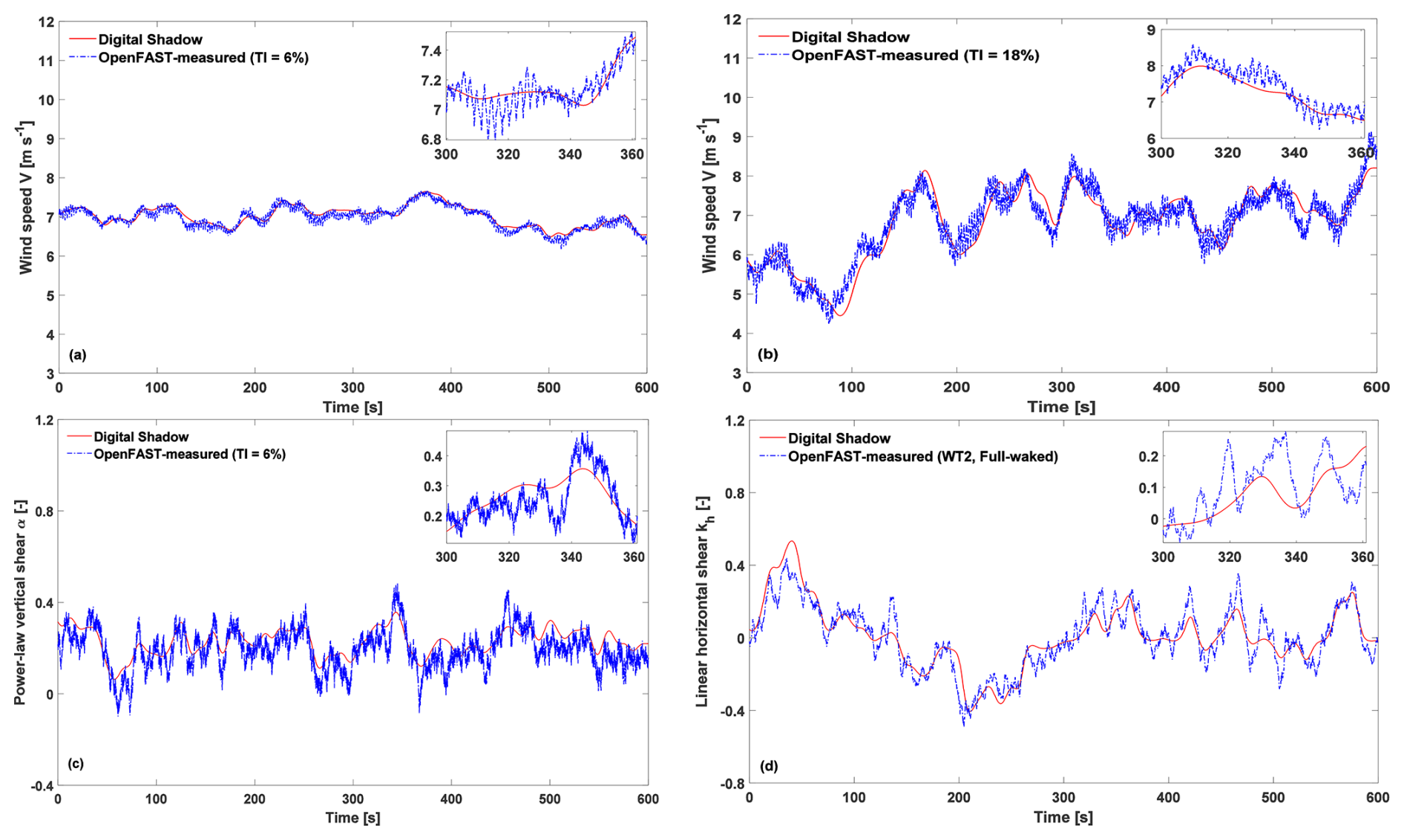
Figure 2 Time histories of the rotor-average wind speed from TurbSim and from Eq. (7) at a wind speed of 7 m s⁻¹ and at TIs of 6 % (a) and 18 % (b), respectively. (c) Time histories of the power-law vertical shear from TurbSim and from Eq. (8), a wind speed of 7 m s⁻¹, and TI equal to 6 %. (d) Time histories of the linear horizontal shear from TurbSim and from Eq. (8) for the downstream turbine in full-waked conditions (see Sect. 3.1.5). Reference results from TurbSim: dashed blue line; estimates: solid red line.

For the same operating condition, Fig. 2c compares the reference power-law vertical shear (dashed blue line) with its estimate from Eq. (8) (solid red line). Figure 2d shows the reference linear horizontal shear and its estimate for a fully waked turbine (Sect. 3.1.5), a case selected because wake meandering induces clear horizontal shear fluctuations, unlike the modest variations typically observed in ambient TurbSim flow fields.

Shear estimation relies on load harmonics obtained via the Coleman–Feingold transformation (Coleman and Feingold, 1958), followed by low-pass filtering (Bertelè et al., 2021). The network also receives the estimated rotor-equivalent wind speed V_E from Eq. (7) and the air density (assumed to be known).

Across all cases, the observers track the ground truth reasonably well but miss some higher-frequency content. This loss is expected, as V_E is inferred from turbine response – filtered by rotor inertia and control action – while the shear observers rely on load harmonics that similarly smooth the blade response. Because these quantities are used solely to schedule (interpolate) the model matrices and equilibrium conditions, omitting high-frequency components is arguably beneficial.

Over the entire range of simulations, the average absolute errors were 2.4 % for wind speed, 14.5 % for the vertical power-law shear exponent, and 11.1 % for the linear horizontal shear. In wake-steering scenarios (Sect. 3.1.5), the mean yaw-misalignment estimation error was 14.5 %.

3.1.3 Performance of the bias-correction approach

To assess the BC approach of Sect. 2.4.1 and examine the roles of the two correction terms, we used the same turbine in a clean low-TI inflow as in Sect. 3.1.2. BC terms were initially disabled to establish the baseline of the uncorrected model. Figure 3a shows tower-top FA deflection from OpenFAST (dashed blue line), the uncorrected digital shadow (solid red line), and the BC-corrected estimate (solid yellow line) at 7 m s⁻¹ and TI of 6 %.

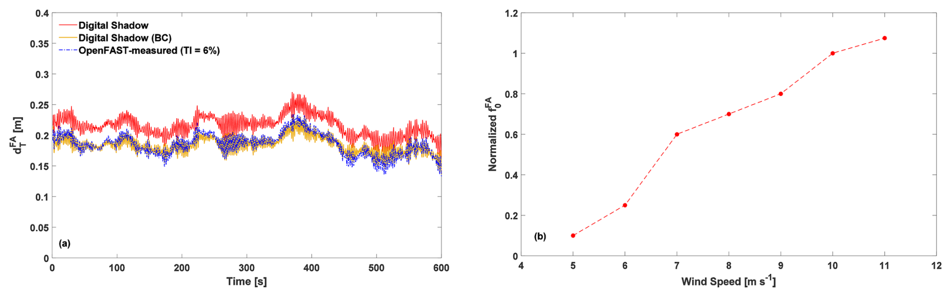
Figure 3 Time histories of tower-top FA deflection as measured on the OpenFAST model (dashed blue line), uncorrected estimates from the digital shadow (solid red line), and corrected estimates using the BC approach (solid yellow line) at a wind speed of 7 m s⁻¹ and a TI of 6 % (a). Variation of the static corrective force ${\mathit{f}}_{\mathrm{0}}^{\mathrm{FA}}$ for the tower-top FA deflection with respect to wind speed (b). The static force is normalized to one at the rated wind speed to highlight relative variations.

Introducing the static corrective force ${\mathit{f}}_{\mathrm{0}}^{\mathrm{FA}}$ reduces the average absolute error from 16.4 % to 2.5 %. Figure 3b illustrates the dependence of this static force on wind speed, normalized to unity at rated wind speed. Similar analyses were performed for other DOFs but are omitted for brevity. The remaining discrepancies between the linear and nonlinear models stem from factors such as shaft tilt, structural deflections, gravity loads, small azimuth differences due to slight rotor-speed deviations (NREL Forum, 2023), and errors in estimating the scheduling vector s.

Bias in blade sensors is common (Pacheco et al., 2024). To assess the effect of the b term for sensor-bias correction (Sect. 2.4.1, Eq. 10c), we artificially added Gaussian noise to the blade 1 strain gauge, with a standard deviation of 0.01 % and a mean equal to 10 % of the mean flapwise bending moment. Figure 4a shows the unbiased OpenFAST measurements (dashed blue line) and the biased ones (dashed teal line). Figure 4b illustrates how b (dashed teal line) converges to the injected bias (solid yellow line), effectively correcting the measurement. Figure 4c compares the blade 1 deflection from the unbiased OpenFAST model (dashed blue line), the biased case (dashed teal line), and the BC-corrected digital shadow (solid yellow line). The average absolute error is 3.61 % without the artificial bias and 3.67 % with compensation, indicating that the correction removes the bias without degrading accuracy. Similar performance was obtained when different biases were applied to each blade sensor.

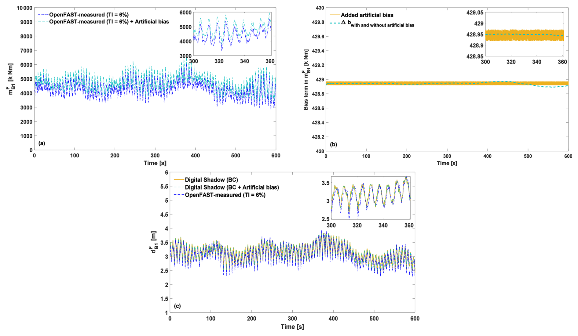
Figure 4 Time histories of blade 1 flapwise bending moment (${\mathit{m}}_{\mathrm{F}}^{\mathrm{B}\mathrm{1}}$) as measured on the OpenFAST model without bias (dashed blue line) and with artificially introduced non-zero Gaussian noise (dashed teal line) (a). Convergence of the term b (dashed teal line) to the mean of the artificially added bias (solid yellow line) (b). Time histories of the estimated blade 1 deflection as measured on the OpenFAST model without bias (dashed blue line), with artificially introduced non-zero Gaussian noise (dashed teal line), and as estimated by the digital shadow using the BC approach (solid yellow line) (c). Results correspond to a wind speed of 7 m s⁻¹ and a TI of 6 %.

3.1.4 Application to a freestream turbine

For the same individual turbine in a clean low-TI inflow of Sect. 3.1.2, Fig. 5a–d show the tower-top FA and SS displacements and the blade tip flapwise and edgewise deflections measured in OpenFAST (dashed blue line) and estimated by the digital shadow with BC (solid yellow line). Figure 5e and f report the tower-base resultant bending moment and the blade resultant bending moment at 15 % span. The figures show a representative case at 7 m s⁻¹ and TI =6 %. Table 1 summarizes the performance across all simulations by listing the average absolute errors.

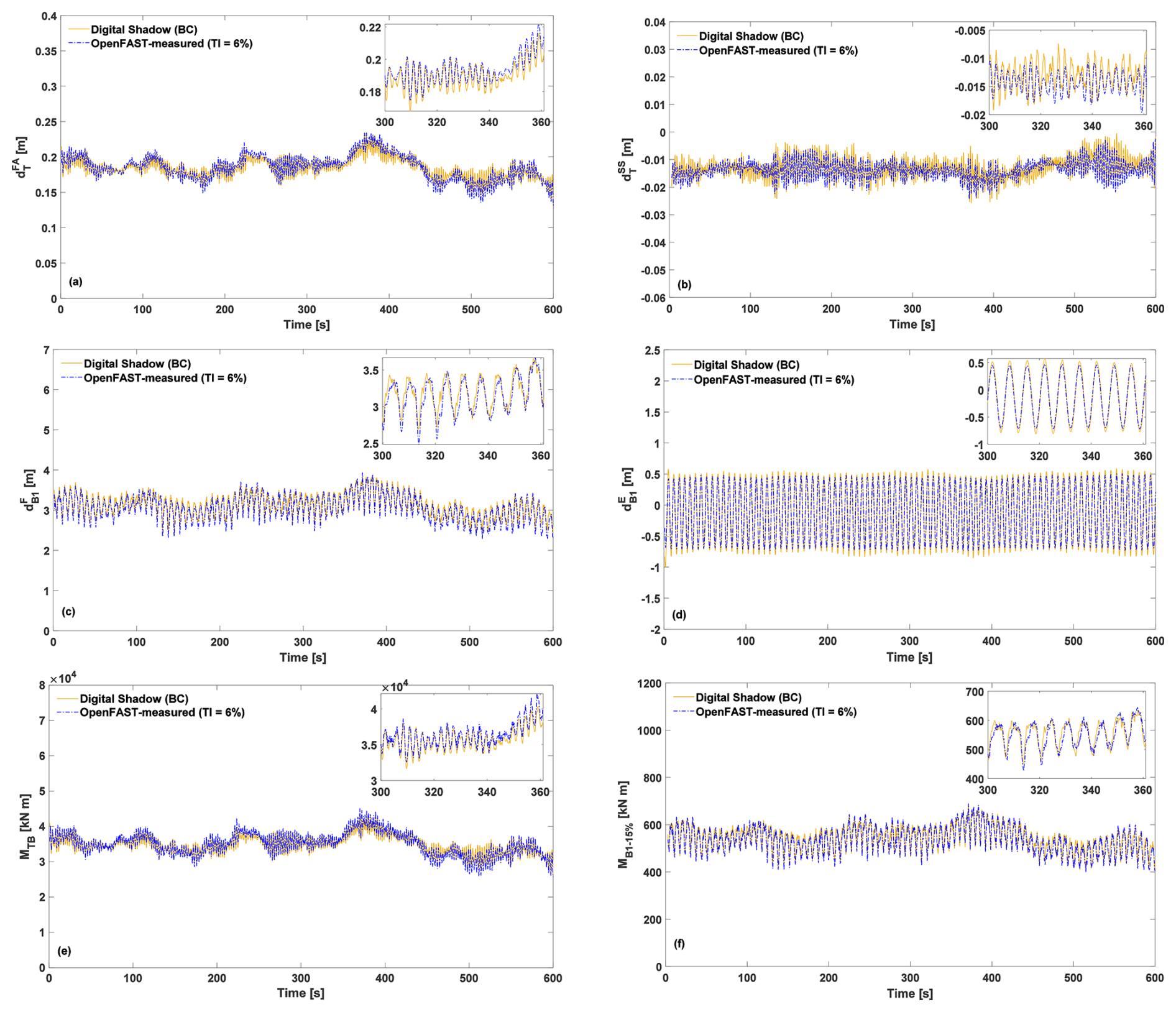
Figure 5 Time histories of tower-top FA deflection (a), tower-top SS deflection (b), and blade tip flapwise (c) and edgewise (d) deflections, tower-base bending moment (e), and blade bending moment at 15 % blade span (f), as measured on the OpenFAST model (dashed blue line) and estimated by the digital shadow using BC (solid yellow line). A wind speed of 7 m s⁻¹ and TI equal to 6 % is considered.

Table 1 Average absolute errors for all conducted simulations for clean inflow conditions.

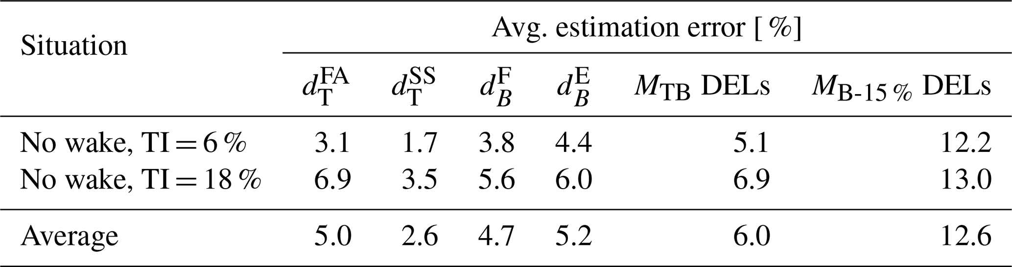
Results show that the average absolute errors of the estimated turbine states remain below 10 % for all simulations. DELs were computed for the tower-base resultant moment M_TB and the blade resultant moment at 15 % span M_B–15 %. Their average absolute errors fall in the 5 %–15 % range, with standard deviations of about 2.7 % for M_TB and 4.5 % for M_B-15 % across all scenarios. As expected, errors increase with TI. The overall error levels are consistent with previous studies (Abdallah et al., 2017; Branlard et al., 2020a, b, 2024a), although those works relied on fewer DOFs and did not include blade dynamics.

3.1.5 Application to waked turbines in a small cluster

To evaluate the method under more complex inflow conditions, we simulated a small turbine cluster using FAST.Farm (Jonkman and Shaler, 2021). The cluster consists of three IEA 3.4-130 RWTs (IEA 3.4-MW Onshore Reference Wind Turbine , 2023) arranged in a row (Fig. 6), denoted as WT1, WT2, and WT3 from upstream to downstream.

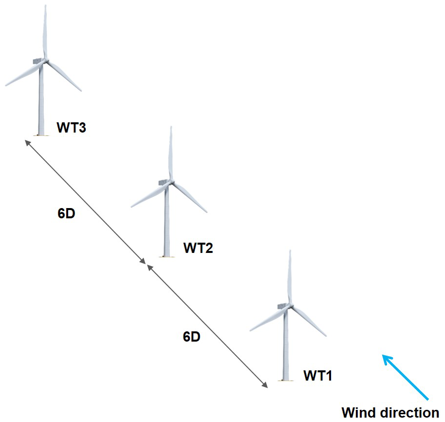
Figure 6 Layout of a small cluster of three IEA 3.4-130 RWTs. For all considered cases, the wind direction (indicated by the blue arrow) is parallel to the row of turbines.

Two scenarios were investigated:

• In the first, WT1 is aligned with the wind at rated speed (9.8 m s⁻¹) and TI =6 %. WT2 lies fully in the wake of WT1, and WT3 in the consecutive wakes of WT1 and WT2. The digital shadow is applied to WT2 and WT3.

• In the second, ambient conditions are the same, but WT1 is yawed by −30°. WT2 is then partially waked by WT1, while WT3 is fully waked by WT2 and partially by WT1. The digital shadow is applied to WT1, WT2, and WT3.

Table 2 summarizes the average absolute errors and DEL estimates for both scenarios. For waked and yawed turbines, blade DEL errors remain comparable to those obtained in Sect. 3.1.4 for a single turbine in high-TI inflow, whereas tower DEL errors are higher. This is consistent with the added wake turbulence impinging on downstream machines. While tower DEL errors are similar for WT1 under yaw misalignment and WT2 under partial waking, blade DEL errors are larger for WT2, likely due to the complex, asymmetric inflow induced by the deflected wake.

Table 2 Average absolute errors of the estimated outputs for all considered situations with complex inflow conditions, encompassing fully, partially, and overlapping waked conditions.

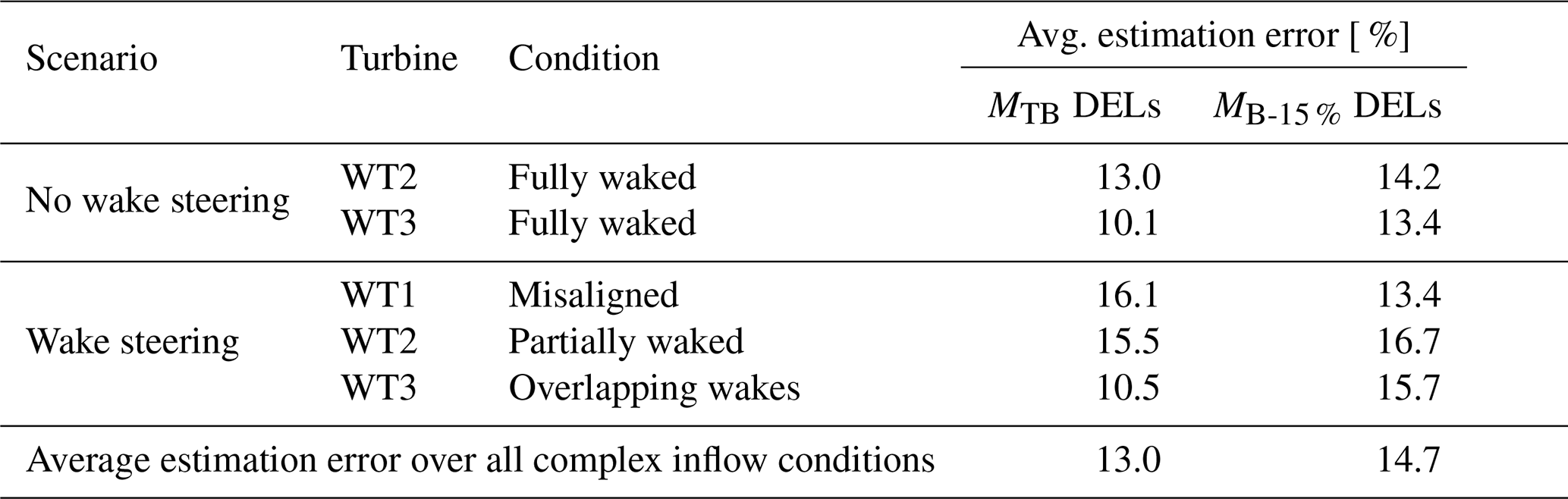
Despite the low ambient TI, tower DEL errors are somewhat larger for the yawed WT1 than for the downstream turbines. This may reflect the complex rotor aerodynamics in yaw, which are not fully captured by the filter-internal model. Moreover, even BEM-based aerodynamics in OpenFAST can be inaccurate in strong yawed-flow conditions (Branlard et al., 2024b), where CFD or free-vortex methods can provide more reliable physics (Boorsma et al., 2018).

To further interpret these results, Fig. 7a–d show the normalized FFT amplitudes of the tower-base bending moment and the blade bending moment at 15 % span for a single turbine in clean inflow and for WT2 in partially waked conditions. OpenFAST measurements (dashed blue line) are compared with digital shadow estimates (solid yellow line). The digital shadow reproduces the main spectral features, particularly around the 1P–3P harmonics, and captures the increase in load amplitudes from aligned to waked inflow. Under waked conditions, OpenFAST peak amplitudes rise by factors of about 5 (tower) and 3 (blade). The digital shadow errors in peak amplitude are 14 % (clean) and 46 % (waked) for the tower-base moment, and 18 % (clean) and 34 % (waked) for the blade moment.

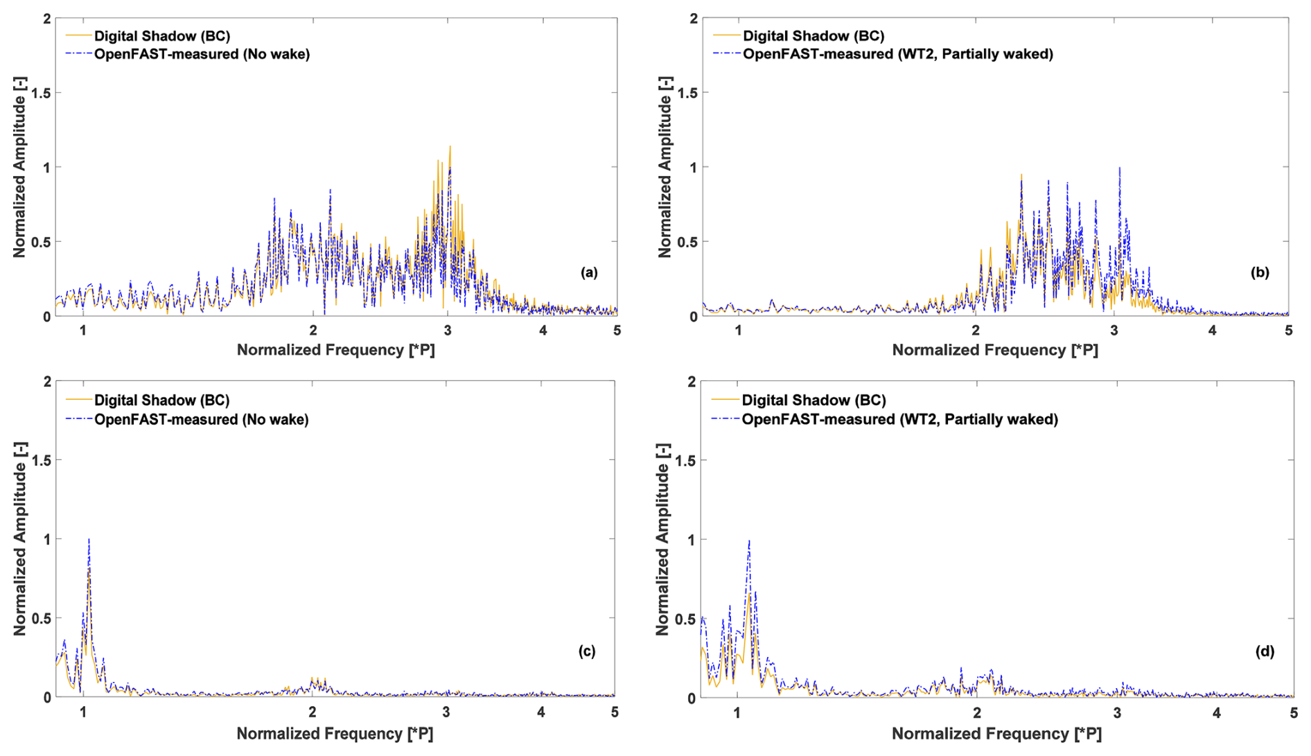
Figure 7 Spectra of the tower-base bending moment (a, b) and the blade bending moment at 15 % blade span (c, d) under clean inflow and partially waked conditions, respectively. The results are shown as measured on the OpenFAST model (dashed blue line) and as estimated by the digital shadow using BC (solid yellow line). The frequencies are normalized by the mean rotor speed, and all FFT amplitudes are scaled relative to the peak amplitude recorded by OpenFAST.

Although the proposed digital shadow is clearly not providing an exact representation of the turbine behavior, the accuracy of the blade response in complex partially waked and misaligned conditions is only slightly worse than the tower response provided by recent simpler digital shadows (Branlard et al., 2020b, 2024b), which would not be applicable in such non-symmetric conditions.

3.2 Validation against field measurements

Next, the digital shadow is evaluated under real-world conditions using measurements from a 3.5 MW eno wind turbine (eno energy GmbH, 2024). Available signals include generator torque, rotor speed, pitch angle, tower-top FA/SS accelerations, and blade-root flapwise and edgewise bending moments, as well as strain-gauge measurements of two components of the tower-base moment and of the blade moment at 25 % span. All data are sampled at 10 Hz. These measurements serve two purposes: (i) to assess the prediction quality of the digital shadow (Sect. 3.2.2); and (ii) to train a data-driven correction of the output model using Eq. (11) (Sect. 3.2.4). Following the procedure of Sect. 2.1, the filter-internal model is built by linearizing an existing OpenFAST model of the turbine over a range of operating points from cut-in to cut-out.

3.2.1 Test site

The dataset used in this study was collected at a test site during two periods (15–30 October 2020 and 23–26 February 2021) as part of an unrelated project. The measurements were used as recorded, without calibration or post-processing, and filtered only to remove gaps, stops, faults, and other non-power-production conditions.

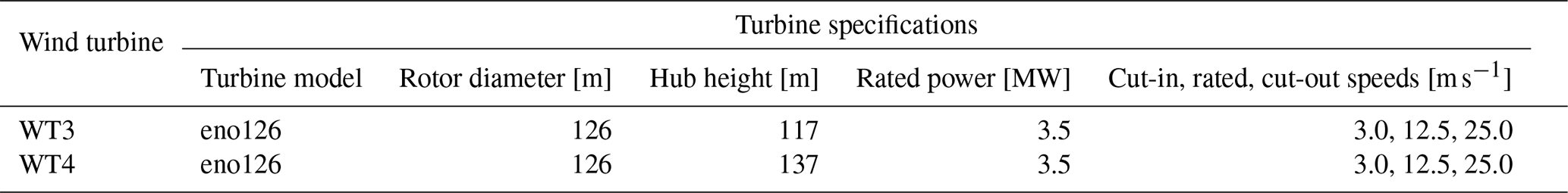
The test site, illustrated in Fig. 8, is located in northeast Germany, near the village of Kirch Mulsow, in the Rostock district of Mecklenburg-Vorpommern, a few kilometers from the Baltic Sea. The terrain comprises gentle hills, open fields, and forests. Four turbines, manufactured by eno energy GmbH (eno energy GmbH, 2024), are installed at the site. The digital shadow was applied to replicate the response of WT3. The main technical specifications of WT3 and WT4 are summarized in Table 4; WT1 and WT2 are not described further, as they played no role in the present experiment.

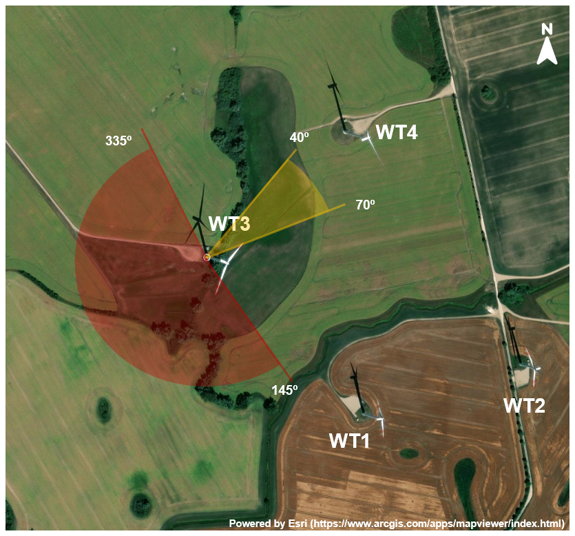
Figure 8 Layout of the test site, showing the turbine locations. The digital shadow is tested for the response of WT3. The sectors highlighted in red and yellow indicate the wind direction range during the testing period, which are characterized by clean freestream and waked conditions, respectively.

Table 3 Inflow conditions during the testing period.

Table 4 Technical specifications of the WT3 and WT4 turbines at the test site.

The testing period was categorized into different inflow conditions, as summarized in Table 3. After filtering out gaps and non-power-production periods, approximately 49 h of clean freestream data were retained. This dataset was split into two subsets: the first 38 h (about 77 %) were used to train the correction approaches described in Sect. 2.4, while the remaining 11 h were kept for validation and correspond to 1 representative day of clean inflow.

Furthermore, as indicated in Table 3, data from selected days with complex inflow were used to evaluate the digital shadow under more challenging conditions. Importantly, no data from complex inflow scenarios were used in tuning the correction terms presented in Sect. 2.4.1.

Wind speed and shear estimators for these turbines were developed and validated in previous studies (Schreiber et al., 2020a; Bertelè et al., 2021).

3.2.2 Digital shadow performance without correction

First, we assess the ability of the digital shadow to estimate quantities of interest when no physical sensors are available. To this end, the digital shadow is fed with SCADA data, blade-root load measurements, and the inflow quantities produced by the wind observers, but not with the tower-base and 25 %-span blade measurements. These withheld measurements are instead used to evaluate the quality of the corresponding estimates.

Figure 9a and b show the normalized measured (dashed blue line) and estimated (solid red line) tower-base bending moment resultant and blade bending moment resultant at 25 % blade span, respectively, over 11 h on a sample day (20 October 2020) under clean freestream conditions, characterized by an average TI of 13.5 % (met mast). The zoomed insets reveal that the digital shadow captures both low- and high-frequency variations well, although a clear offset is present due to the plant/internal-model mismatch between the real turbine and the approximate aeroelastic model – an effect not observed in the simulated study of Sect. 3.1.4, where the same OpenFAST model served as both plant and filter-internal model.

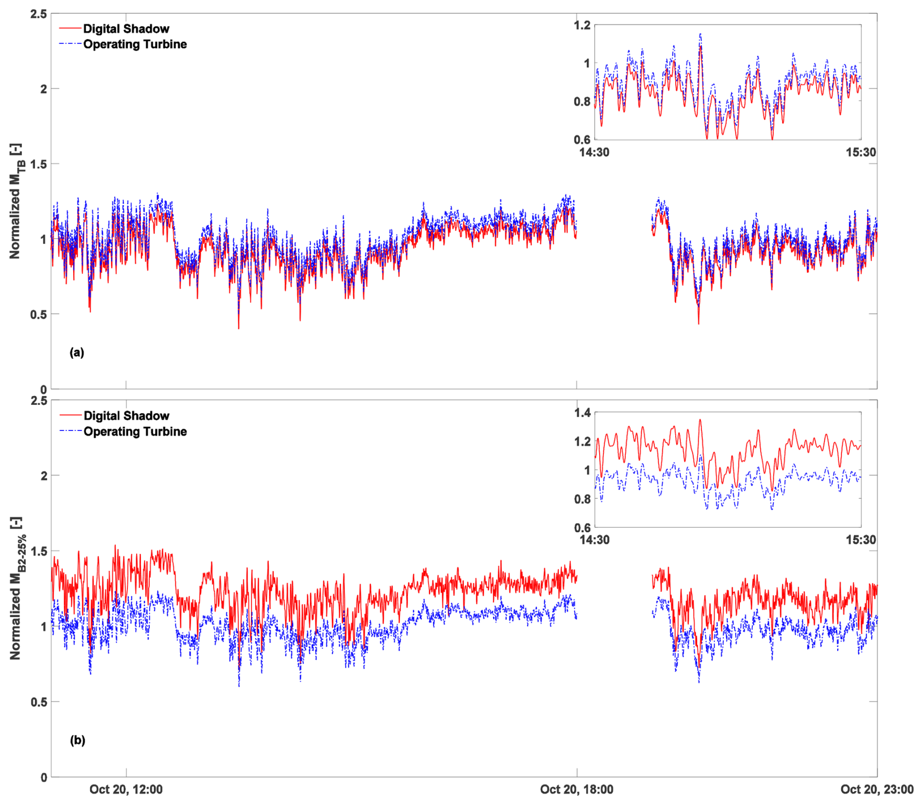
Figure 9 Time histories of tower-base bending moment (a) and blade bending moment at 25 % blade span (b), as measured (dashed blue line) and estimated by the digital shadow (solid red line) for 11 h on a sample day (20 October 2020) in the available dataset under clean freestream conditions. All values have been normalized using the same factor to preserve the confidentiality of the turbine data.

For this sample day, the average absolute errors are 5.9 % for the tower-base bending moment resultant and 21.3 % for the 25 %-span blade bending moment resultant. Over the full training dataset, the tower-base error averages 12.4 % (min: 9.7 %, max: 19.7 %), while the 25 %-span blade error averages 18.7 % (range: 13.7 %–23.7 %).

3.2.3 Virtual sensing (bias correction)

Second, to remove the observed offset, the correction of both outputs and states is performed using the BC approach described in Sect. 2.4.1 and based on Eq. (10). The tuning of the correction terms followed the procedure of Sect. 3.1.3, relying on tower-top and blade-root measurements collected during the testing period.

First, the static force term f₀ was adjusted through an iterative tuning process until no further improvement was obtained. This term was found to depend mainly on wind speed, whereas the other scheduling variables s had negligible influence under clean freestream conditions. While a manual tuning strategy was adopted in this work, more systematic or automated optimization approaches (e.g., gradient-based, Bayesian, or heuristic methods (Nocedal and Wright, 2006)) could be employed and represent a promising direction for future development. Next, the bias term b was activated, and its driving process noise was tuned to further reduce measurement errors. As with the process noise affecting the dynamic equilibrium equations, no significant dependency on wind speed or turbulence intensity was observed. After tuning, the average absolute errors over the training dataset were 3.1 % for the tower-top acceleration resultant and 3.5 % for the blade-root bending moment resultant.

Table 5 summarizes the average absolute errors and output DELs for the full dataset, grouped by the inflow classes defined in Table 3. For the same sample day shown in Fig. 10, the bias correction reduces the average absolute errors for M_TB and M_B-25 % to 4.2 % and 2.7 %, respectively, indicating that the offset has been effectively removed. The corresponding DEL estimation errors are 4.3 % for M_TB and 9.1 % for M_B-25 %. Overall, the BC approach accurately tracks both low- and high-frequency fluctuations, providing reliable DEL estimates for the quantities of interest.

Table 5 Overview of average absolute errors and estimated output DELs under various inflow conditions.

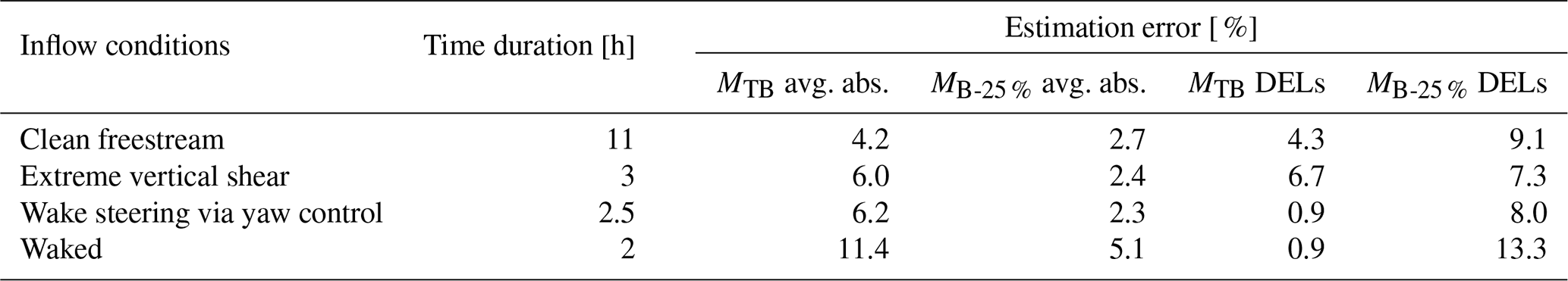
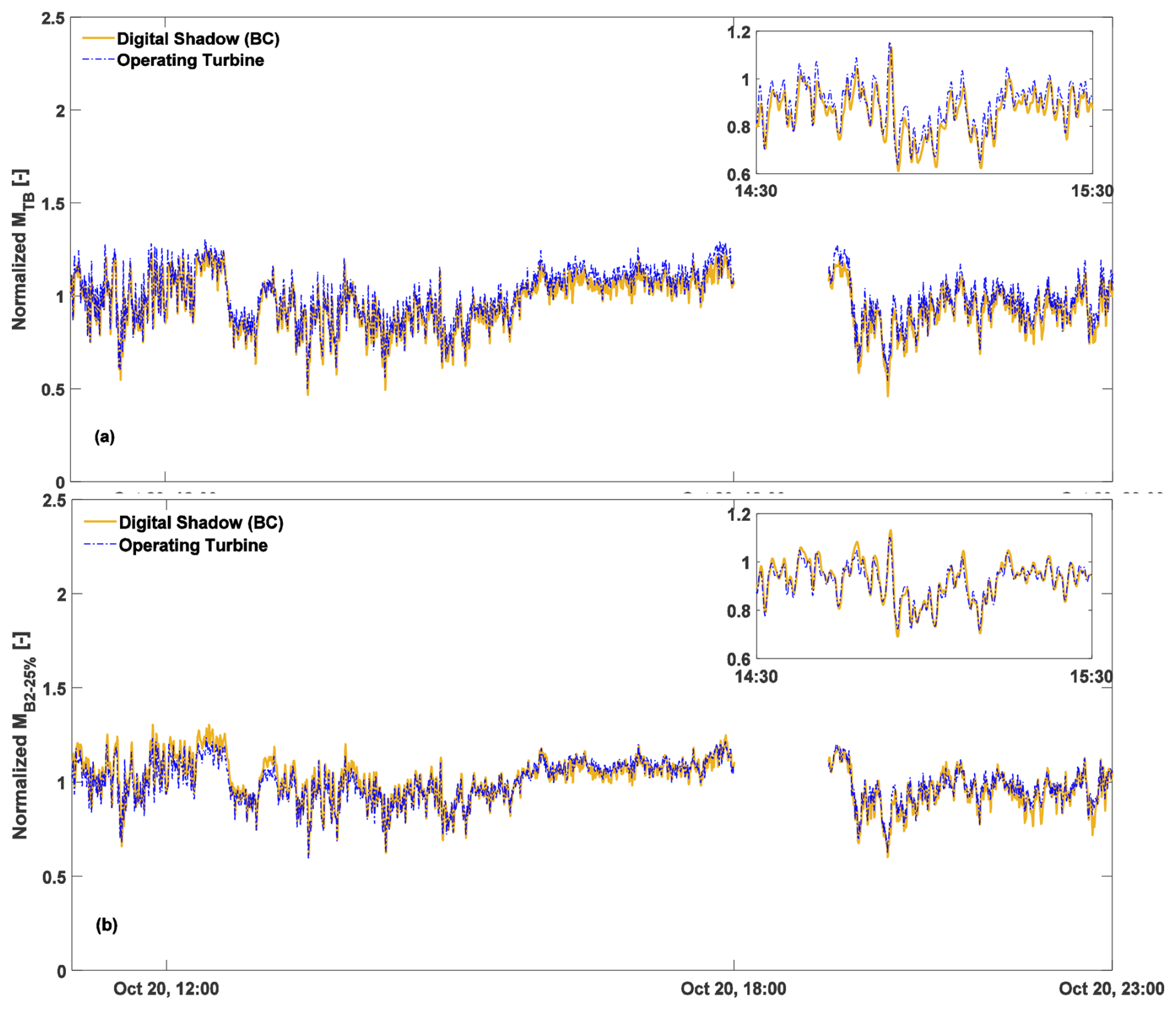
Figure 10 Time histories of the tower-base bending moment (a) and blade bending moment at 25 % blade span (b) for 11 h on a sample day (20 October 2020) in the available dataset under clean freestream conditions. Measurements: dashed blue line; corrected estimates of the digital shadow using BC: solid yellow line. All values have been normalized using the same factor to preserve the confidentiality of the measured turbine data.

It is worth noting that the BC method proves more effective in the field than in the simulation environment. This may stem from the higher TI and the tenfold faster sampling rate used in simulations, which introduces additional high-frequency fluctuations that are harder to estimate accurately.

Given the strong and generalizable performance of the BC approach, all remaining results for complex inflow conditions are obtained using this method. This choice also aligns with a key application of the digital shadow as a virtual sensor for quantities that cannot be directly measured for technical or economic reasons. For brevity, time-history plots are shown only for the waked inflow case (Fig. 11), as this scenario is particularly informative regarding model behavior under complex aerodynamic interactions. Figures for the other inflow classes are omitted for conciseness.

• Extreme vertical shear. The BC correction – tuned exclusively on the training dataset defined in Table 3 – was developed without using any complex inflow data. Even so, the average absolute errors for M_TB and M_B-25 % are 6.0 % and 2.4 %, respectively, for the extreme vertical shear dataset. The corresponding DEL estimation errors are 6.7 % and 7.3 %. These results confirm that the BC approach maintains errors below 10 % even under severe shear conditions, where the power-law exponent ranges from 0.15 to 0.72 (average 0.42).

• Wake steering via yaw control. For the wake-steering scenario, the average absolute errors for M_TB and M_B-25 % are 6.2 % and 2.3 %, respectively, while the DEL estimation errors are 0.9 % and 8.0 %. Yaw misalignment varies between −16 and 11°. Despite the inherently more complex dynamics associated with wake steering, the digital shadow continues to perform robustly under these conditions.

• Waked. Figure 11a through d show the tower-base bending moment, the 25 %-span blade bending moment resultant, and the vertical and horizontal shears for the waked dataset. Measurements are shown as dashed blue lines, and BC-corrected estimates as solid yellow lines. The power-law vertical shear has an average value of −0.15 (dashed dark-red line), attributed to the higher hub height of WT4 and its wake influence on WT3. The horizontal shear averages −0.12 (dashed light-red line), further confirming strongly waked conditions.

  For this dataset, the average absolute errors for M_TB and M_B-25 % are 11.4 % and 5.1 %, respectively, while the DEL estimation errors are 0.9 % and 13.3 %. Although the BC approach generally performs well, the complex turbine dynamics and large variations in vertical and horizontal shear under wake conditions result in slightly higher errors, with some values exceeding 10 %.

  Overall, the range of average estimation errors is consistent with the findings of previous studies (Abdallah et al., 2017; Branlard et al., 2020a, b, 2024a), which relied on fewer DOFs and neglected blade dynamics, and were not validated under complex inflow.

  While the digital shadow remains effective under all tested conditions, the slightly higher errors in complex inflow suggest that further refinement could be achieved with a larger dataset. In particular, the tuning of the BC correction terms may benefit from explicitly incorporating – in addition to wind speed – also variations in vertical and horizontal shear and yaw misalignment.

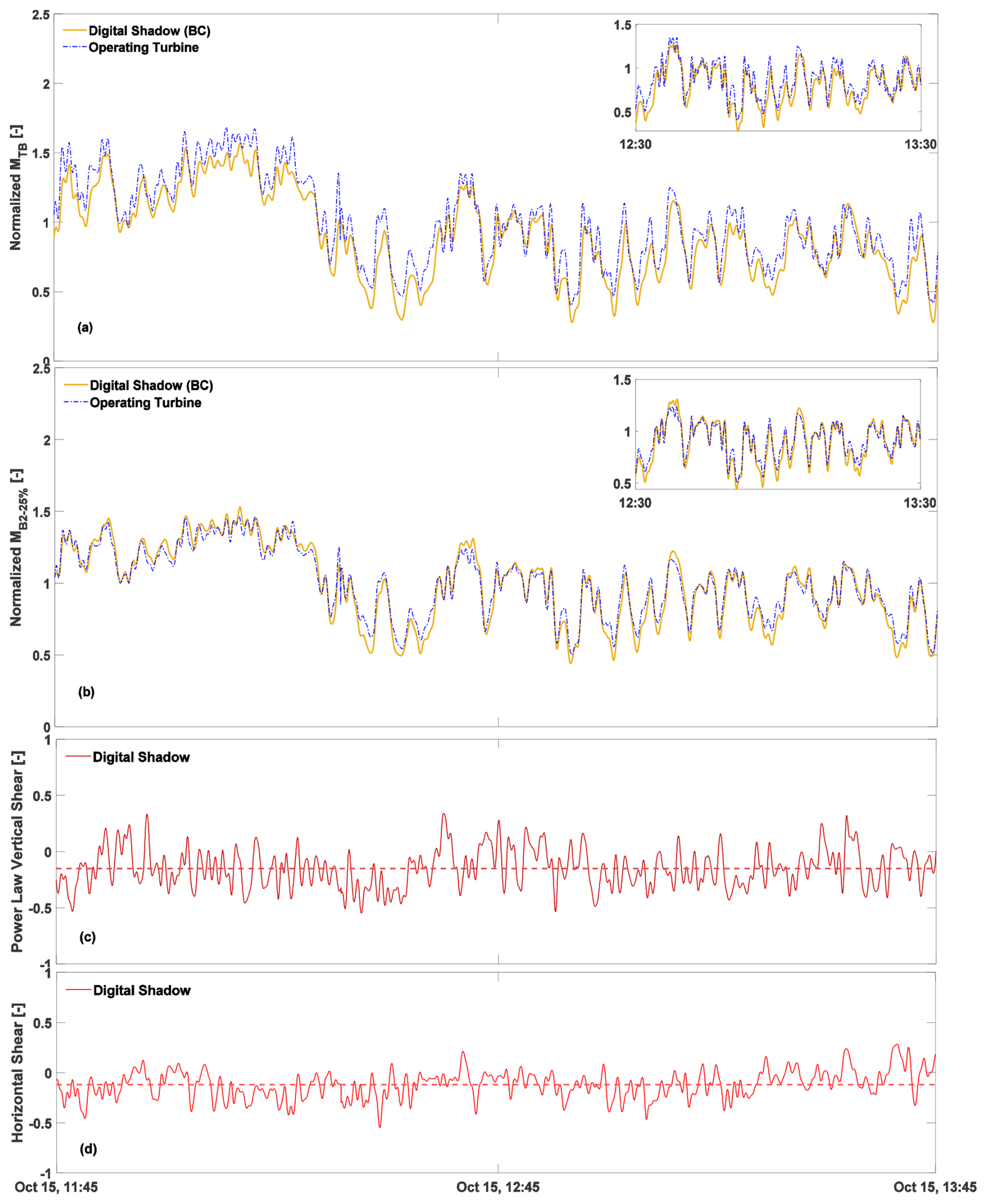
Figure 11 Time histories of the tower-base bending moment (a), blade bending moment at 25 % blade span (b), vertical shear (c), and horizontal shears (d). Measurements: dashed blue line; corrected estimates of the digital shadow using BC: solid yellow line. The shears are shown with solid red lines, with an average value marked by dashed red lines. All values have been normalized using the same factor to preserve the confidentiality of the measured turbine data.

3.2.4 Condition monitoring

Next, measurements of the tower-base and 25 %-span blade bending moments were used to implement and validate a data-driven a posteriori correction of the corresponding output equations, following Eq. (11), to obtain high-quality predictions of these quantities. In this configuration, the turbine is permanently instrumented, and the digital shadow provides expected values under the current operating conditions. A CM activity (not further discussed here) may then compare predictions and measurements to detect anomalies. Prediction quality is quantified using the root mean squared percentage error (RMSPE), commonly adopted in CM (Liu et al., 2023).

The same dataset used in Sect. 3.2.2 was employed, with a sample day reserved for validation. The NN-based correction term was implemented using the MATLAB Deep Learning Toolbox (The MathWorks, Inc., 2022). A basic trial-and-error study led to a neural network with one hidden layer of 16 neurons. During training, the Polak–Ribiére conjugate gradient algorithm (traincgp) and Broyden–Fletcher–Goldfarb–Shanno (BFGS) quasi-Newton backpropagation (trainbfg) yielded the best performance for the tower-base and 25 %-span blade bending moment, respectively. The resulting RMSPEs during training were approximately 0.8 % for the tower-base and 0.9 % for the 25 %-span blade bending moment.

Figure 12a and b reports time histories of the tower-base and 25 %-span blade bending moment resultants, respectively. Measurements are shown with a dashed blue line and the corrected estimates with a solid green line. Before implementing the a posteriori error correction, the RMSPE for M_TB and M_B-25 % were 6.1 % and 21.6 %, respectively. After data-driven correction, these values dropped to 1.3 % and 1.5 %, respectively.

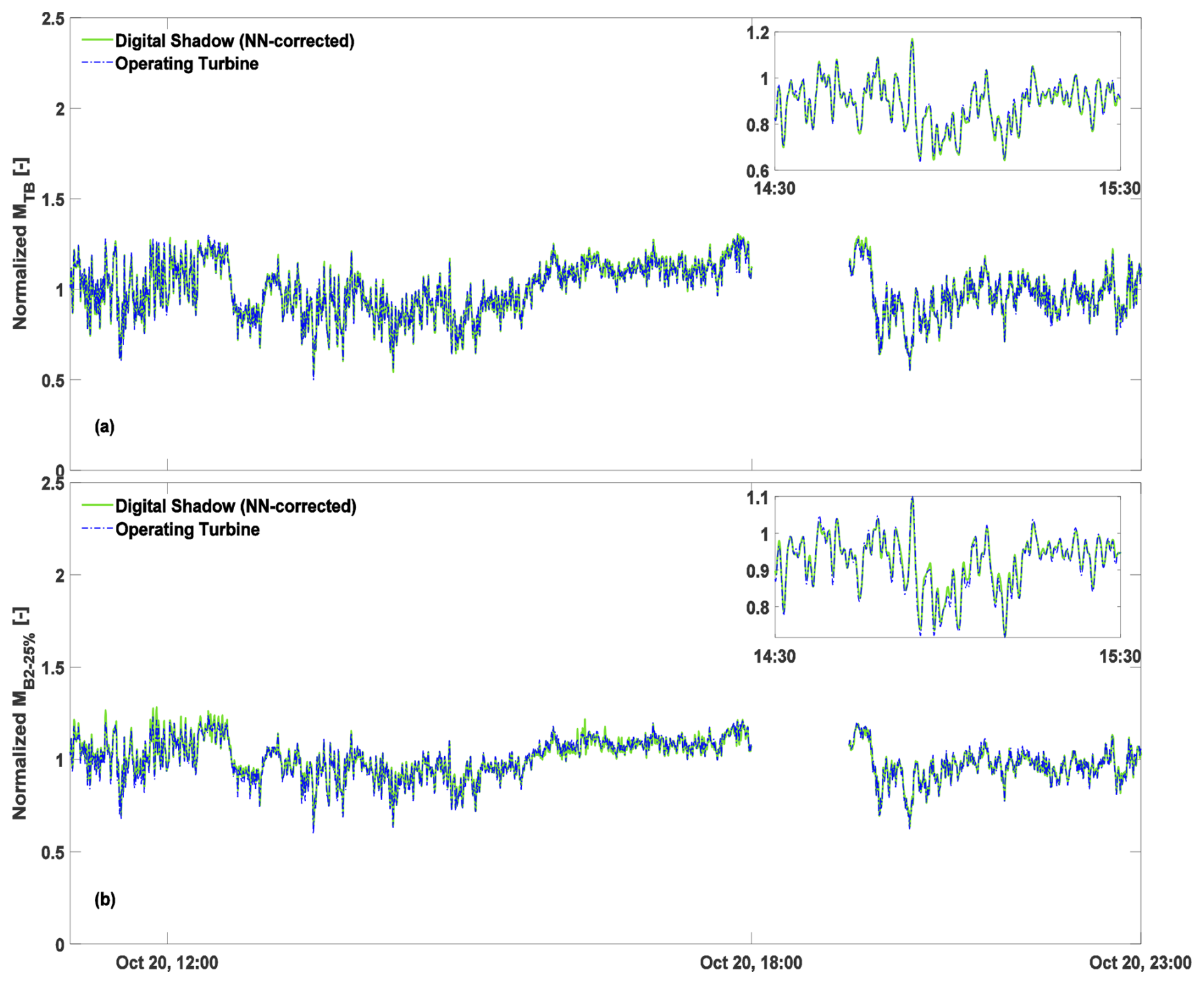
Figure 12 Time histories of the tower-base bending moment (a) and blade bending moment at 25 % blade span (b). Measurements: dashed blue line; corrected estimates of the digital shadow using NN: solid green line. All values have been normalized using the same factor to preserve the confidentiality of the measured turbine data.

A closer inspection of the time series also shows that the NN-corrected model captures most of the short-term intermittency present in the measured loads, including the majority of fast fluctuations driven by turbulent inflow. The sharpest intermittent spikes observed in real turbine data are only partially reproduced, reflecting the inherent smoothing of the underlying linear model. Nevertheless, the dominant variability and overall intermittency level are matched well enough for the CM application considered here. Overall, it appears that the proposed data-driven approach is highly effective in correcting the output equations, as both slow and fast fluctuations of the two quantities of interest are tracked with remarkable accuracy, although it cannot improve the state model.

4 Conclusions

We have presented, verified, and validated a digital shadow of a wind turbine, first in a simulation environment under freestream, waked, and wake-steering scenarios, and then against a field dataset. Building on a classical Kalman filtering framework, the approach linearizes an existing and trusted aeroservoelastic model to derive the filter-internal linear model. Reusing such models reduces development time, leverages prior tuning and validation efforts, increases confidence in results, and avoids duplication of work.

Departing from existing studies, tower side–side and rotor blade DOFs were included to support more general operating conditions, such as sheared inflow, waked flow, and yaw misalignment. Since the linearization must now span a broader solution space, the filter-internal model is scheduled with respect to parameters representing the main drivers of the turbine response. These scheduling parameters are estimated in real time using the rotor-as-a-sensor technology from SCADA and blade-load measurements.

Simulation testing showed state-estimation errors generally below 10 % across all conditions. DEL errors ranged from 5 % to 15 %, with higher values under elevated turbulence and waked inflow, as expected. Slightly larger errors (16.1 %) occurred under yaw misalignment, reflecting limits of the linearized model. Field results were remarkably similar to those in simulation, even without ad hoc tuning, although clear biases indicated limitations of the underlying filter-internal model.

A key limitation of a digital shadow is its dependence on a white state-space model, which is inevitably affected by modeling errors. To address this, two alternative data-driven correction strategies were examined, yielding gray models with substantially improved prediction accuracy.

The BC approach performed robustly under complex inflow conditions, including extreme vertical shear, waked flow, and wake-steering control. Errors remained small in all cases, demonstrating strong reliability and adaptability. Overall, the BC method reduced average absolute errors from roughly 20 % to 2 %–11 %, and DEL estimation errors to 1 %–13 %. This represents a significant improvement over recent literature and underscores its potential for fatigue analysis, lifetime estimation, and load-aware control. In parallel, the NN-based a posteriori output correction proved highly effective, reducing load RMSPE from 10 %–15 % to about 1 %, which is particularly promising for CM applications.

Several improvements are possible. Additional inflow quantities may further enhance scheduling of the filter-internal model; for instance, veer could be included and estimated using rotor-as-a-sensor technology by extending the harmonic content to 2P (Bertelè et al., 2024). Validation should also be expanded to larger field datasets covering broader inflow and operating conditions, as well as different turbine types. Moreover, the tuning of the BC correction term could be refined by accounting for variations in vertical and horizontal shear, as well as yaw misalignment, which would require more extensive data. We also note that the wind speed and shear observers smooth some high-frequency content; however, since these quantities are used solely for model scheduling, this limitation has limited practical impact.

Appendix A: Nomenclature

b	Vector of sensor biases
f0	Static correction force
i	Input vector of the inflow estimator
m	Vector of bending moments
p	Vector of free network parameters
q	Vector of generalized displacements
s	Vector of scheduling parameters
u	Input vector
v	Vector of generalized velocities
y	Vector of outputs for Kalman innovation
z	Vector of other outputs of interest
ν	Measurement noise vector
ω	Process noise vector
A	Rotor-swept area
c	Generic output of the wind inflow
	observer
Cp	Power coefficient
d	Displacement
J	Rotor inertia
kh	Horizontal shear
M	Bending moment resultant
m	Bending moment component
Q	Torque
R	Rotor radius
V	Wind speed
α	Vertical power-law shear exponent
γ	Misalignment angle
ϵ	Output correction term
θ	Blade pitch angle
λ	Tip-speed ratio
ρ	Air density
ψ	Rotor azimuthal position
Ω	Rotor rotational speed
(⋅)E	Edgewise component
(⋅)F	Flapwise component
(⋅)FA	Fore–aft component
(⋅)SS	Side–side component
(⋅)IP	In-plane component
(⋅)OP	Out-of-plane component
(⋅)NN	Quantity corrected by a neural network
(⋅)1c	1P cosine component
(⋅)1s	1P sine component
(⋅)Bi	Quantity referred to the ith blade
(⋅)B-s %	Quantity referred to the s % spanwise location
(⋅)TB	Quantity referred to the base of the tower
(⋅)E	Estimated quantity
(⋅)M	Measured quantity
(⋅)0	Reference equilibrium condition
δ(⋅)	Perturbation about a reference equilibrium
	condition

BEM	Blade element momentum
CFD	Computational fluid dynamics
CM	Condition monitoring
DEL	Damage-equivalent load
DOF	Degree of freedom
FA	Fore–aft
FEM	Finite element method
FFT	Fast Fourier transform
LUT	Lookup table
NN	Neural network
BC	Bias correction
PSD	Power spectral density
RMSPE	Root mean squared percentage error
ROM	Reduced-order model
RWT	Reference wind turbine
SCADA	Supervisory control and data acquisition
SS	Side–side
TI	Turbulence intensity
WT	Wind turbine