Sub-minute fatigue monitoring for enhanced lifetime assessment of wind turbines

Accurate fatigue-damage estimation is a critical step for managing and extending the life of wind turbine fleets and the basis on which operators decide whether an ageing asset can be kept in service beyond the end of design life. The most accurate estimation relies on continuous high-frequency strain measurements processed with rainflow cycle counting. However, only a small subset of turbines within a fleet are typically instrumented with strain sensors, and even for these, the data volumes, computational complexity, and cost of continuously processing high-frequency strain data via rainflow counting over long-term operation make this approach impractical to sustain at scale. For this reason, industry practice has long relied on stress data aggregated over 10 min windows already used by supervisory control and data acquisition (SCADA) systems, which are available across the full fleet. This choice is convenient but, when combined with conventional window-based rainflow counting, tends to underestimate fatigue damage generated by cycles whose period exceeds the window length, driven by factors such as slow variations in wind speed and direction, operational transitions, control actions, and seasonal or daily temperature variation, as well as, for offshore turbines, changes in wave parameters. Residual-preserving approaches, most notably low-frequency fatigue dynamics (LFFD), address this limitation by reconstructing cycles that span window boundaries but have so far been applied almost exclusively within the conventional 10 min framework.

Technology has recently enabled operators to deploy second-resolution SCADA metrics at scale and at reasonable cost, offering finer-grained statistical descriptors for applications such as load and bending-moment estimation and operational-state classification. This is also an opportunity to revisit fatigue monitoring at a SCADA-aligned timescale that is short enough to limit the truncation of boundary-spanning cycles inherent to conventional window-based counting yet aggregated enough to remain deployable across large fleets. This paper benchmarks the families of methods that make this opportunity actionable against continuous rainflow as a baseline: conventional window-based counting, a modified low-frequency fatigue dynamics (LFFD) formulation that explicitly resolves intra-window and inter-window damage contributions, and two reduced-information extrema-sequence representations – start–peaks–valleys–end (SPVE) and maximum and minimum (max–min). The evaluation uses 6 months of 15 s windows of SCADA and strain measurements acquired at 50 Hz from two instrumented tower sections of an onshore wind turbine and examines the influence of window length, sampling rate, and fatigue-curve formulation on damage computation (Eurocode 3 vs. DNV).

Reducing the aggregation window from 10 min to 15 s alone does not improve fatigue estimation, as shorter windows increasingly truncate the low-frequency cycles that dominate accumulated damage. The proposed modified LFFD framework overcomes this limitation by preserving cycle continuity across window boundaries, recovering 99.5 % of the baseline damage while requiring only a fraction of the original data volume. Reduced-information representations further demonstrate that fatigue can be estimated with high accuracy using strongly compressed stress sequences, with start–peaks–valleys–end (SPVE) and maximum and minimum (max–min) retaining 98.8 % and 96.2 % of the baseline damage, respectively. These findings establish a practical pathway towards SCADA-aligned, data-efficient fatigue monitoring, enabling scalable lifetime assessment across large wind turbine fleets while preserving the fidelity of high-resolution structural measurements.

1 Introduction

Wind turbine structures are subjected to highly variable loading arising from stochastic aerodynamic forcing, control actions, grid interactions, and frequent transitions between operational states (IEC 61400-13, 2015; Pacheco et al., 2022; Pacheco, 2022). These excitations generate cyclic stresses in structural components, leading to progressive fatigue damage, one of the governing mechanisms for structural reliability and lifetime consumption (Marsh, 2016; Marsh et al., 2016; Pacheco et al., 2022; Pacheco, 2022). Accurate fatigue assessment is therefore central to certification, lifetime extension, and risk-informed asset management, particularly for ageing fleets operating under conditions that may deviate from design assumptions (IEC 61400-12-1, 2005; IEC 61400-13, 2015; Pacheco et al., 2022; Pacheco, 2022).

In practice, fatigue monitoring relies on strain measurements that are discretised into conventional 10 min windows, following both design-basis load simulation practice and the aggregation format of supervisory control and data acquisition (SCADA) systems (IEC 61400-13, 2015). These windows, aligned with long-established standards and certification procedures, typically provide statistical descriptors (means, standard deviations, extrema) of operational variables (IEC 61400-13, 2015). However, many fatigue-driving events occur on substantially shorter timescales, including rapid control adjustments, transient aerodynamic loading, and operational state changes (Marsh, 2016; Marsh et al., 2016; Pacheco et al., 2022; Pacheco, 2022). When these 10 min statistical descriptors, rather than the full strain signal, are used as a proxy for fatigue-relevant loading, this aggregation may therefore smooth short-term stress fluctuations and distort the underlying cycle distribution, potentially biasing fatigue estimates (Marsh, 2016; Marsh et al., 2016).

Wind turbine manufacturers increasingly provide higher-frequency SCADA data at sub-minute intervals (Pacheco et al., 2022; Sadeghi et al., 2022, 2023). This development creates the opportunity to reassess fatigue monitoring strategies at shorter, SCADA-consistent timescales (Sadeghi et al., 2022, 2023). The objective is not to physically segment structural dynamics into artificial intervals but to evaluate whether fatigue-relevant cycle information, especially large-amplitude cycles associated with slow variations in mean load and operational transitions, can be reliably preserved when stress data are aggregated at sub-minute resolution, enabling scalable monitoring without storing continuous high-frequency measurements. In this study, a 15 s window is adopted as the sub-minute aggregation interval, as this corresponds to the native temporal resolution at which the high-frequency SCADA data are available for the instrumented turbine.

Residual-preserving approaches, most notably the low-frequency fatigue dynamics (LFFD) methodology, address this limitation by extracting closed cycles within each window and reconstructing boundary-spanning cycles by concatenating residual stress sequences (Amzallag et al., 1994; Marsh, 2016; Marsh et al., 2016). Previous studies have demonstrated that this procedure preserves equivalence with continuous rainflow cycle counting (RFC) while enabling window-based processing (Marsh, 2016; Marsh et al., 2016). However, existing applications have been formulated and validated almost exclusively within the conventional 10 min windowing framework, and fatigue damage has typically been reported in aggregate form without explicit separation of cycle contributions arising within and across windows (Faria et al., 2024; Marsh, 2016; Marsh et al., 2016; Sadeghi et al., 2022, 2023). This explicit separation enables a more granular characterisation of fatigue behaviour and, as shown later in this study, is particularly relevant when the window length is reduced below the conventional 10 min duration, since the low-frequency residual contribution then accounts for the majority of total fatigue damage.

In addition to residual-based approaches, reduced-information strategies based on extrema extraction have been proposed to reduce storage and computational demand requirements. By retaining only representative turning points per window (e.g. start–peaks–valleys–end or maximum–minimum values), these methods aim to preserve the sequence information required for rainflow cycle counting (RFC) while substantially compressing the input signal (Larsen and Thomsen, 1996; Shah et al., 2025, 2026). Although extrema-based representations have been explored in the context of low-frequency fatigue effects, their performance has not been systematically benchmarked against residual-preserving methods using experimental tower strain data and sub-minute windows (Faria et al., 2024; Larsen and Thomsen, 1996; Sadeghi et al., 2022, 2023; Shah et al., 2025, 2026).

Previous experimental and simulation-based studies have shown that neglecting low-frequency fatigue dynamics can lead to a systematic underestimation of accumulated fatigue damage in wind turbine structures (Faria et al., 2024; Larsen and Thomsen, 1996; Marsh, 2016; Marsh et al., 2016; Sadeghi et al., 2022, 2023; Shah et al., 2025). Deviations reported between conventional 10 min window-based rainflow counting and approaches that preserve cycle continuity typically range from approximately 8 % to more than 60 %, depending on operating conditions, structural components, and fatigue-curve formulation (Faria et al., 2024; Larsen and Thomsen, 1996; Marsh, 2016; Marsh et al., 2016; Sadeghi et al., 2022, 2023; Shah et al., 2025). A consistent trend across the literature is the strong dependence of this bias on the adopted Wöhler exponent m, as fatigue damage becomes increasingly dominated by relatively rare but large-amplitude stress excursions associated with slow variations in mean load and operational transitions (Larsen and Thomsen, 1996; Sadeghi et al., 2022, 2023). For welded steel tower details represented by bi-linear σ−N formulations with slopes $m=\mathrm{3}/\mathrm{5}$, reported low-frequency contributions are typically on the order of 20 %–40 % of total fatigue damage (Faria et al., 2024; Sadeghi et al., 2022, 2023), indicating that standard 10 min windows may lead to materially non-conservative lifetime estimates. These findings highlight the need for fatigue monitoring strategies that preserve low-frequency cycle effects while remaining compatible with short, SCADA-aligned windows suitable for large-scale deployment (IEC 61400-13, 2015; Marsh, 2016; Marsh et al., 2016).

Despite the growing availability of high-frequency operational and structural data, three key gaps remain. First, the influence of reducing windows below 10 min on tower fatigue, as estimated from long-term field strain measurements, has not been comprehensively quantified. Second, although low-frequency fatigue dynamics (LFFD) frameworks have been applied in several studies, their capability to explicitly separate and characterise high- and low-frequency fatigue contributions (in the pragmatic monitoring sense adopted here), together with the associated cycle-count and damage spectra, has not been demonstrated using long-term wind turbine measurements, even within the conventional 10 min framework. Third, the accuracy–storage trade-off of reduced-information extrema sequences has not been systematically evaluated relative to rainflow-equivalent residual-preserving methods using experimental data.

To address these gaps, this study presents a comprehensive evaluation of fatigue monitoring methodologies using 6 months of high-frequency strain data from two instrumented tower sections of an onshore wind turbine. Continuous rainflow cycle counting (RFC) is adopted as baseline and compared with (i) conventional window-based rainflow counting, (ii) a modified low-frequency fatigue dynamics (LFFD) implementation that explicitly separates intra-window (predominantly high-frequency) and inter-window (predominantly low-frequency) fatigue contributions through residual-sequence reconstruction, and (iii) reduced-information extrema sequence methods. The analysis investigates the influence of window length, sampling rate, and the selected σ−N curve model used for damage calculation on accumulated damage, cycle spectra, and computational and storage requirements.

In this work, fatigue contributions are classified as high-frequency, corresponding to intra-window cycles (closing within a window), and low-frequency fatigue associated with inter-window cycles (spanning multiple windows and reconstructed through residual concatenation). This terminology is methodological and refers solely to signal segmentation; it does not represent a spectral decomposition of turbine loading processes. A physically high-frequency structural cycle may be categorised as inter-window if truncated by window boundaries.

The principal objective of this work is to enable fatigue assessment at a higher level of temporal granularity, extending beyond cumulative damage estimation alone. Here, granularity refers to both the temporal discretisation of the stress signal and the explicit separation of fatigue contributions into intra-window and inter-window components. By resolving these contributions across different window lengths and analysing the associated cycle-count and damage spectra, the study provides (i) a quantitative benchmark of window- and sampling-driven deviations relative to continuous rainflow counting, (ii) a structured decomposition of fatigue into high-frequency (intra-window) and low-frequency (inter-window) fatigue contributions, and (iii) an accuracy–storage–computation comparison of residual-preserving and extrema-based representations. Together, these results establish a practical basis for SCADA-aligned, data-efficient fatigue monitoring suitable for wind-farm-scale deployment and lifetime extension applications.

A preliminary version of part of this analysis, restricted to 1 month of data and to the high-/low-frequency LFFD partitioning with simple value-sequence representations, was presented at the TORQUE conference (Oliveira et al., 2026). The present work substantially extends it through a 6-month dataset, the continuous rainflow baseline, the max–min representation, the EC3–DNV comparison, and the accuracy–storage–computation benchmark.

This paper is structured as follows. Section 2 presents the fatigue-damage estimation methodologies considered in this study, including continuous rainflow cycle counting (RFC) as baseline, window-based approaches, the residual-preserving low-frequency fatigue dynamics (LFFD) framework, and reduced-information extrema-sequence methods, together with the metrics used for quantitative comparison. Section 3 introduces the experimental dataset and case study, describing the instrumented wind turbine, the measurement campaign, and the signal pre-processing steps. Section 4 presents and discusses the experimental results, analysing the influence of sampling rate and fatigue-curve formulation on cumulative damage, the effect of window length on fatigue partitioning, and a systematic comparison of all monitoring methods in terms of accuracy, data storage, and computational requirements. Finally, Sect. 5 summarises the main findings and discusses their implications for scalable, SCADA-aligned fatigue monitoring and lifetime assessment of wind turbine towers.

2 Fatigue-damage estimation methodologies

2.1 Continuous rainflow cycle counting (baseline counting method)

When continuous strain measurements are available, fatigue assessment can be performed by applying rainflow cycle counting (RFC) directly to the full, unsegmented stress time series (Amzallag et al., 1994; Matsuishi and Endo, 1968; McInnes and Meehan, 2008). By preserving the complete sequence of stress reversals, this approach provides the most accurate reconstruction of the fatigue spectrum, including both full and half cycles (Fig. 1a–b).

In this work, continuous rainflow cycle counting (RFC) applied to the full stress history is adopted as the baseline fatigue assessment against which all alternative methodologies are benchmarked. Although computationally demanding and therefore impractical for long-term operational monitoring at scale, it provides a consistent and objective baseline for quantifying the effect of signal window length, residual processing, and information reduction (Marsh, 2016; Marsh et al., 2016).

2.2 Window-based high-frequency-cycle counting

In practice, fatigue assessment of wind turbine towers is commonly based on fixed-duration windowing, typically using 10 min windows in accordance with IEC 61400-13 (IEC 61400-13, 2015). In this approach, the stress time series is segmented into consecutive windows of equal duration (Fig. 1c), and rainflow cycle counting (RFC) is applied independently to each window (Fig. 1d). Cycle counts, including full and half cycles, are then aggregated across windows to obtain cumulative fatigue damage (Fig. 1e). While widely adopted, window-based high-cycle counting exhibits an inherent limitation: stress excursions that span multiple windows are truncated at window boundaries. This truncation leads to the loss of large-amplitude, long-period cycles associated with slowly varying mean stresses, resulting in non-conservative fatigue life estimates when such cycles contribute significantly to damage (Marsh, 2016; Marsh et al., 2016).

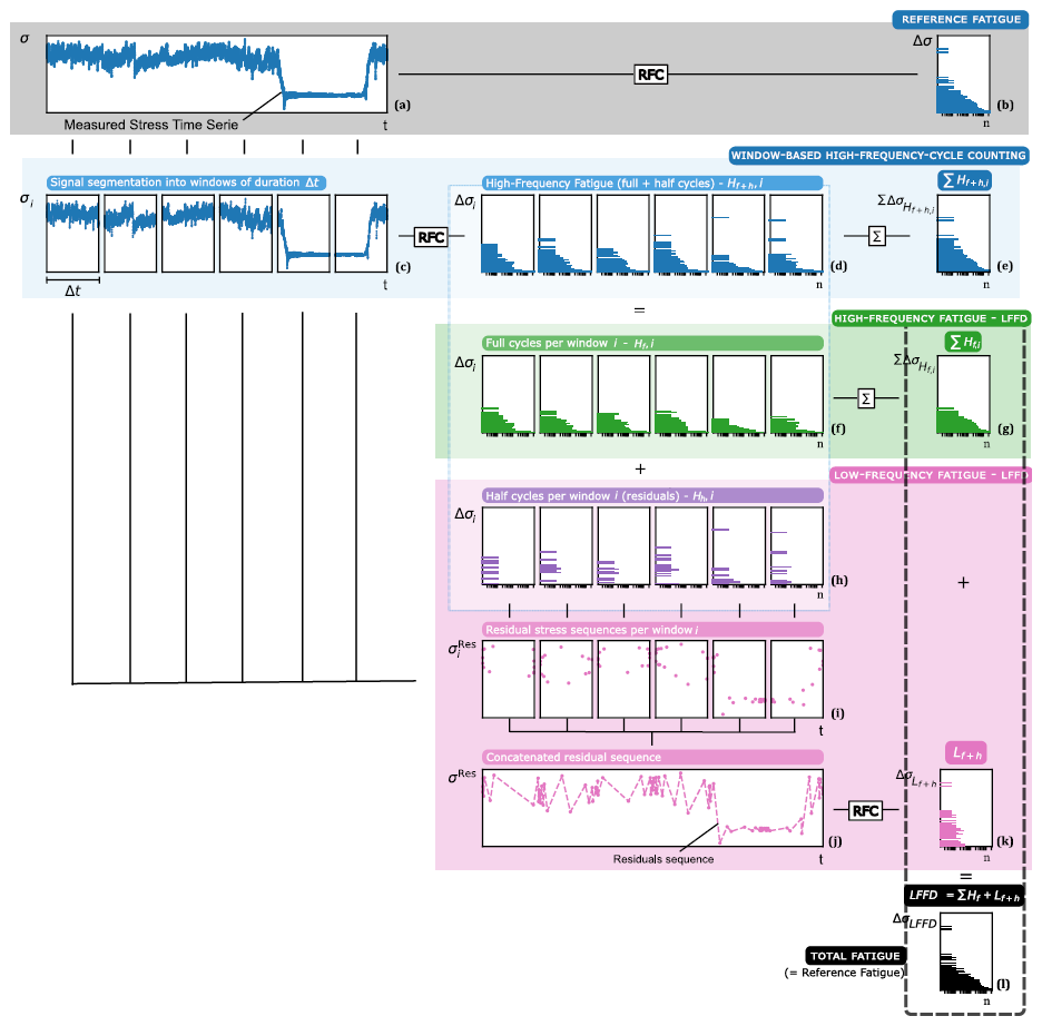
Figure 1 Overview of fatigue monitoring methodologies based on rainflow cycle counting (RFC). (a) Measured stress time series. (b) Baseline fatigue spectrum obtained by applying RFC to the full signal, including full and half cycles. (c) Segmentation of the stress time series into consecutive windows of duration Δt. (d) RFC applied independently to each window, yielding window-level fatigue spectra. (e) Aggregated fatigue spectrum obtained by summing full and half cycles across all windows. (f) Full cycles extracted within each window. (g) Aggregated full-cycle spectrum representing the high-frequency, window-contained fatigue contribution. (h) Half cycles remaining in each window. (i) Residual stress sequences associated with unclosed half cycles. (j) Concatenation of residual stress sequences across windows. (k) RFC applied to the concatenated residual sequence, capturing low-frequency fatigue cycles spanning multiple windows. (l) Total fatigue spectrum obtained by combining the high-frequency (full-cycle) and low-frequency (residual-based) contributions, preserving equivalence with continuous RFC.

2.3 Low-frequency fatigue dynamics (LFFD)

Residual-preserving fatigue analysis originates from the formalisation of rainflow cycle counting (Amzallag et al., 1994), which introduced the residual sequence to represent unclosed stress excursions after cycle extraction. The importance of long-period loading effects in wind turbine fatigue was subsequently highlighted by Larsen and Thomsen, who showed that large-amplitude cycles associated with operational transitions can disproportionately contribute to fatigue damage, particularly for higher Wöhler exponents (Larsen and Thomsen, 1996). To avoid artificial cycle closure and double counting inherent to conventional window-based approaches, Marsh et al. (2016) demonstrated that extracting closed cycles within each window and concatenating the remaining residual sequences preserves equivalence with continuous rainflow counting (Marsh, 2016; Marsh et al., 2016). This residual-preserving framework, later termed low-frequency fatigue dynamics (LFFD), has since been validated using long-term wind turbine strain measurements and shown to capture fatigue contributions that are otherwise systematically underestimated (Faria et al., 2024; Sadeghi et al., 2022, 2023; Shah et al., 2025, 2026).

Within this framework, rainflow cycle counting (RFC) is first applied independently to each window to extract closed cycles (Fig. 1f). The remaining unclosed stress excursions are retained as residual stress sequences (Fig. 1h–i), which are concatenated across windows (Fig. 1j) and subsequently processed using rainflow cycle counting (RFC) to recover cycles spanning multiple windows (Fig. 1k). The resulting fatigue response can be expressed as the sum of two contributions: a high-frequency contribution associated with cycles fully contained within individual windows, and a low-frequency contribution associated with cycles reconstructed from the concatenated residual sequence. Their combination is equivalent to the fatigue spectrum obtained using continuous rainflow cycle counting (RFC) (Fig. 1l), thereby preserving rainflow equivalence (Marsh, 2016; Marsh et al., 2016).

In this study, a modified low-frequency fatigue dynamics (LFFD) implementation is adopted to explicitly quantify high- and low-frequency fatigue contributions while maintaining equivalence with the baseline method (Fig. 2). This explicit separation enables a more granular characterisation of fatigue behaviour and is particularly relevant when the window length is reduced below the conventional 10 min duration.

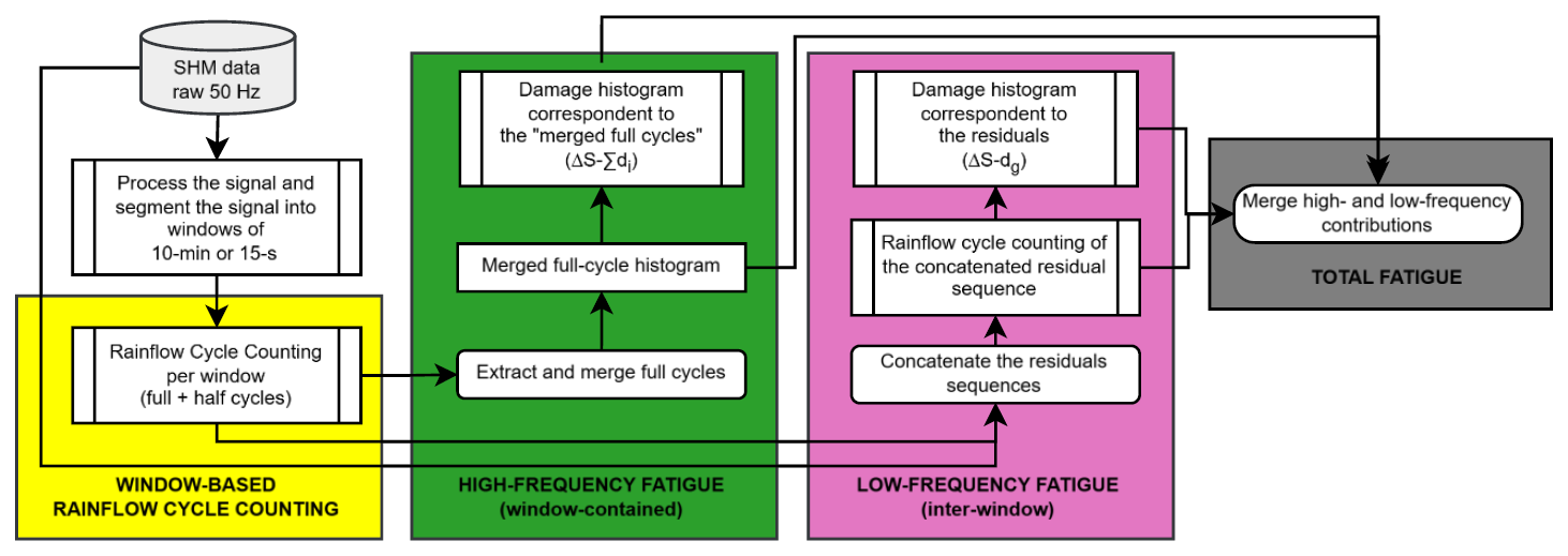
Figure 2 Simplified flowchart of the modified low-frequency fatigue dynamics (LFFD) methodology, inspired in Faria et al. (2024), Sadeghi et al. (2022). Following signal pre-processing and windowing, rainflow cycle counting (RFC) is applied independently within each window. High-frequency fatigue (green) is obtained from merged full-cycle histograms, while low-frequency fatigue (pink) is derived from RFC applied to concatenated residual sequences across windows. Damage and cycle-count histograms are computed separately for each contribution and subsequently merged to obtain the total fatigue response (grey), preserving equivalence with continuous rainflow counting. The link from the raw SHM data to the residual-concatenation step reflects the need for the original, temporally ordered stress values of the unclosed excursions, which are not retained in the half-cycle counts alone.

2.4 Extrema sequence methods

Rainflow counting is inherently sequence dependent, relying solely on the order and magnitude of stress turning points (Amzallag et al., 1994; Matsuishi and Endo, 1968; McInnes and Meehan, 2008). This property motivates reduced information fatigue representations in which the full stress time series is replaced by a simplified sequence of representative extrema, substantially reducing data volume and computational effort.

Two extrema-based representations are considered in this work (Fig. 3). The start–peaks–valleys–end (SPVE) approach retains, for each window, the start, peaks, valleys, and end values of the stress signal (Fig. 3b). Concatenation of these points forms a continuous extrema sequence (Fig. 3c), to which rainflow cycle counting (RFC) is applied once to identify fatigue cycles, including those spanning multiple windows (Fig. 3d).

A further reduction is achieved using the maximum–minimum (max–min) approach, which retains only the maximum and minimum stress values within each window (Fig. 3e–f). This representation emphasises large-amplitude, long-period stress variations associated with operational transitions and enables extreme data compression with minimal computational cost (Larsen and Thomsen, 1996; Shah et al., 2025, 2026).

Extrema sequence methods are examined here as reduced information representations that complement, rather than replace, residual-preserving approaches. Their performance is evaluated relative to continuous rainflow cycle counting (RFC) and low-frequency fatigue dynamics (LFFD) in terms of fatigue accuracy, window length, and data handling efficiency.

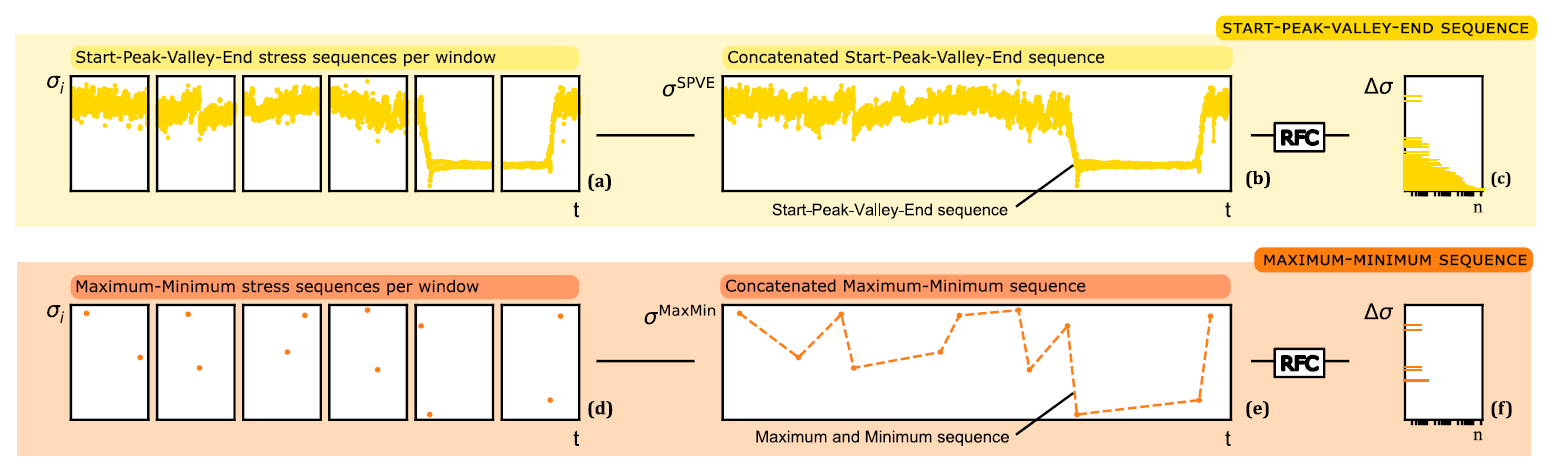
Figure 3 Extrema sequence methods for reduced-information fatigue assessment. (a) Windowed extraction of start, peaks, valleys, and end (SPVE) points within each window. (b) Concatenation of the windowed SPVE values to form a continuous start–peaks–valleys–end sequence; rainflow cycle counting (RFC) is applied to identify fatigue cycles, including those spanning multiple windows. (c) Resulting fatigue spectrum obtained from the SPVE sequence. (d) Windowed extraction of maximum and minimum stress values per window. (e) Concatenation of windowed maxima and minima to form a maximum–minimum (max–min) sequence; rainflow cycle counting (RFC) is applied to identify fatigue cycles. (f) Resulting fatigue spectrum obtained from the max–min sequence. The SPVE approach preserves local turning-point structure, while the max–min approach provides a highly compressed representation emphasising large-amplitude, long-period stress variations.

2.5 Metrics for fatigue evaluation

To establish a consistent and quantitative comparison between fatigue assessment methodologies for wind turbine towers, this study evaluates performance based on five complementary dimensions: (i) the relative contribution of low- and high-frequency fatigue-damage components, (ii) sensitivity of fatigue-damage estimates to the adopted design standard, (iii) sensitivity to signal temporal resolution (sampling rate and window length), (iv) agreement of alternative monitoring methodologies with a baseline fatigue assessment, and (v) data reduction quantification.

Fatigue assessment in the present work is based on the evaluation of accumulated fatigue damage, under the assumption of linear damage accumulation with the number of applied load cycles at each stress level (Pacheco et al., 2022; Pacheco, 2022). Accordingly, the Palmgren–Miner linear damage accumulation rule (Kauzlarich, 1989; Miner, 1945) is adopted, whereby the total fatigue damage is obtained by summing the individual damage contributions associated with all stress ranges over the entire time series:

$$\begin{array}{}\text{(1)}& D=\sum _{i=\mathrm{1}}^{n_{\mathit{\sigma }}}{\displaystyle \frac{n_i}{N_i}},\end{array}$$

where i denotes the ith stress range bin, n_i is the number of cycles counted at the stress range σ_i, and N_i is the corresponding number of cycles to failure.

Two σ−N curve formulations are considered: EC3 (Eurocode 3) detail category 80 and DNVGL-RP-C203 welded-steel, both using a bi-linear σ−N curve with slopes $m=\mathrm{3}/\mathrm{5}$.

All fatigue-monitoring approaches compared in Sect. 4 apply the damage formulation of Eq. (1) to a cycle spectrum (n_i, Δσ_i) and differ only in how this spectrum is obtained from the measured stress signal. Continuous RFC (Sect. 2.1) applies rainflow counting directly to the full stress time series and is adopted as the baseline. Window-based RFC (Sect. 2.2) applies rainflow counting independently within each aggregation window, discarding cycles whose turning points span window boundaries. LFFD (Sect. 2.3, Fig. 2) recovers these boundary-spanning cycles by additionally applying RFC to the concatenated sequence of unclosed half-cycles (residuals) left at each window boundary, combining this low-frequency contribution (L_f+h) with the within-window, high-frequency contribution (H_f+h) to recover the continuous-RFC spectrum exactly. SPVE and max–min (Sect. 2.4, Fig. 3) instead replace the full stress time series within each window by a small set of representative extrema, start–peaks–valleys–end, or maximum/minimum, respectively, before a single RFC pass is applied to the concatenated extrema sequence.

The specific metrics adopted in this work and their mathematical definitions are summarised in Table 1, which provides a structured overview of the performance indicators used throughout the analysis together with the associated equation numbers. These metrics are applied consistently in the following sections to enable objective comparisons across monitoring methodologies, temporal resolutions, and modelling assumptions.

Table 1 Overview of fatigue-damage metrics adopted in the present study.

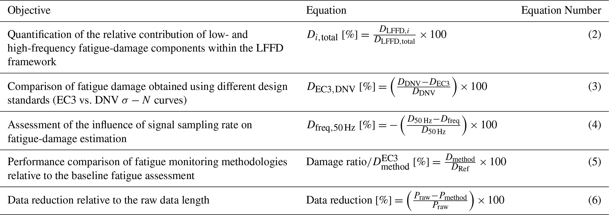
where:
– D_i,total is the percentage contribution of component i, with i∈{low, high}, to the total fatigue damage. D_LFFD,total is the total damage obtained by the LFFD methodology.
– D_LFFD,i is the fatigue damage of component i.
– D_DNV is the fatigue damage computed using DNVGL-RP-C203 curve.
– D_EC3 is the fatigue damage computed using EC3 curve, category 80.
– D_50 Hz is the fatigue damage computed from the baseline signal sampled at 50 Hz.
– D_freq is the fatigue damage computed from the signal decimated with the data sampling rate freq, with $\text{freq}=\left\{\mathrm{6.25},\mathrm{12.5},\mathrm{25}\right\}\left[Hz\right]$.
– $D_{\mathrm{method}}^{\mathrm{EC}\mathrm{3}}$ is the fatigue damage estimated for each method under evaluation, with $\text{method}=\left\{L_{f+h},\mathrm{SPVE},\max -\min ,H_{f+h}\right\}$
– D_Ref is the baseline fatigue damage estimated considering a continuous rainflow cycle counting (RFC) of the signal, without segmentation.
– P_raw is the number of points that belong to the raw signal.
– P_method is the number of the points that belong to the sequence signal for each method, with $\text{method}=\left\{L_{f+h},\mathrm{SPVE},\max -\min \right\}$.

3 Case study and experimental data

The wind farm is a multi-megawatt onshore installation located along a mountain ridge crest in central Portugal. The wind turbines are arranged in an elongated quasi-linear layout along the ridge over karstic highly irregular terrain that, combined with heterogeneous land cover, induces non-uniform wind flow and locally enhanced turbulence.

The dataset used in this study combines SCADA operational and environmental data with measurements from a structural health monitoring (SHM) system installed on a wind turbine with an 90 m rotor diameter. The SHM system instruments two tower sections, T1 and T2, located approximately 54 and 71 m above ground level, respectively (Fig. 4a). Each section is equipped with four circumferential resistive strain gauges (S1–S4) and one PT100 temperature sensor (Fig. 4b–c). Although accelerometers are also available, they are not considered in the present work. All SHM channels were sampled at 50 Hz.

Given the ridge-crest, quasi-linear turbine layout, wake interactions with neighbouring turbines are expected for wind directions aligned with the ridge axis, potentially increasing unsteady thrust loading. As this study is based on strain measurements from a single instrumented turbine, a quantitative assessment of wake effects on tower fatigue was beyond the scope of the present dataset.

The monitoring campaign started in September 2023 and has remained operational continuously since then. In this study, a 6-month subset covering the period between November 2023 and April 2024 is analysed. This period was selected to capture representative variability in operational and inflow conditions (Fig. 4d–e) while also satisfying the minimum duration recommended by IEC guidelines for measurement-based fatigue assessment (IEC 61400-13, 2015).

The raw measurements were pre-processed according to the procedures described in IEC 61400-12-1 (2005) and IEC 61400-13 (2015) and related references (HBM, 2022; IEC 61400-13, 2015; Pacheco et al., 2022; Pacheco, 2022). The processing workflow includes temperature compensation, sensor calibration, strain-to-stress conversion, decomposition into fore–aft (FA) and side-to-side (SS) components using the high-frequency yaw signal, decimated identically to the strain measurements and therefore matching the native temporal resolution of the analysed data, and IEC-based wind-speed correction. To enable consistent comparisons across different sampling frequencies, the strain signals were low-pass filtered using an eighth-order Butterworth filter and subsequently decimated to 25, 12.5, and 6.25 Hz.

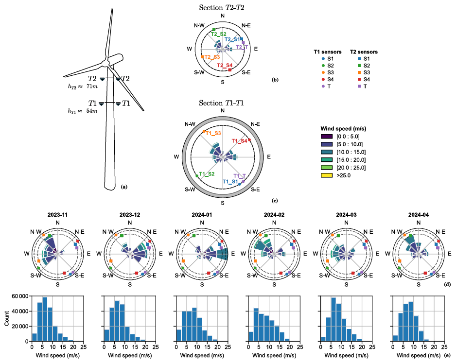
Figure 4 Turbine instrumentation and inflow conditions. (a) Instrumented tower sections T1 and T2. (b–c) Sensor layout at each section (strain gauges S1–S4 and temperature sensor T). (d) Monthly wind roses and (e) wind speed histograms for November 2023–April 2024.

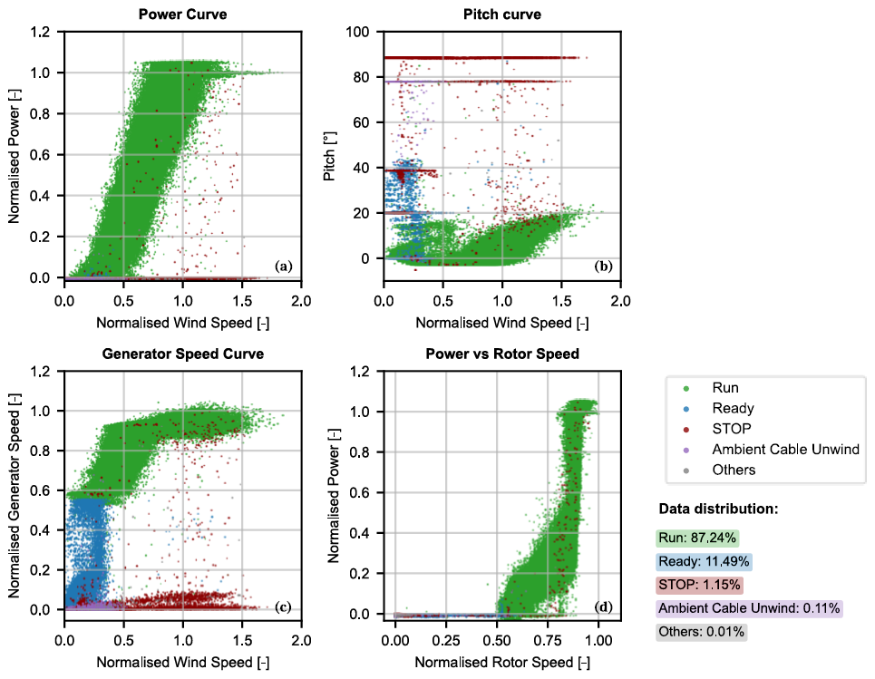
Figure 5 SCADA operational curves for the study period (15 s data). (a–c) Normalised power, pitch, and generator-speed curves versus normalised wind speed. (d) Normalised power versus normalised rotor speed. Colours indicate operational status; the right panel shows the sample distribution by status.

Figure 5 summarises the wind turbine's operational behaviour during the analysed period and provides context for the strain-based fatigue assessment. Figure 5a–d present the relationships between power, pitch angle, generator speed, rotor speed, and wind speed. The data points are coloured according to the turbine operational status, including Run (actively producing power), Ready (available and connected, awaiting sufficient wind or dispatch conditions to start producing), STOP (intentionally stopped, whether by manual command, scheduled maintenance, or a triggered safety/fault condition), Ambient Cable Unwind, and other less frequent states.

The dataset is dominated by normal turbine operation, with the Run state accounting for 87.24 % of all samples. The Ready state accounts for an additional 11.49 %, while the remaining operational states correspond to only a small fraction of the dataset. This distribution confirms that the analysed period is primarily characterised by standard power-production conditions, with relatively limited occurrence of shutdown or transient operational events.

4 Analysis of experimental data

4.1 Stress–damage (Δσ−D) representations

Fatigue results are commonly represented using stress–cycle (Δσ−N) distributions. In the present work, stress–damage (Δσ−D) distributions are additionally employed to highlight the stress ranges that dominate fatigue-damage accumulation explicitly.

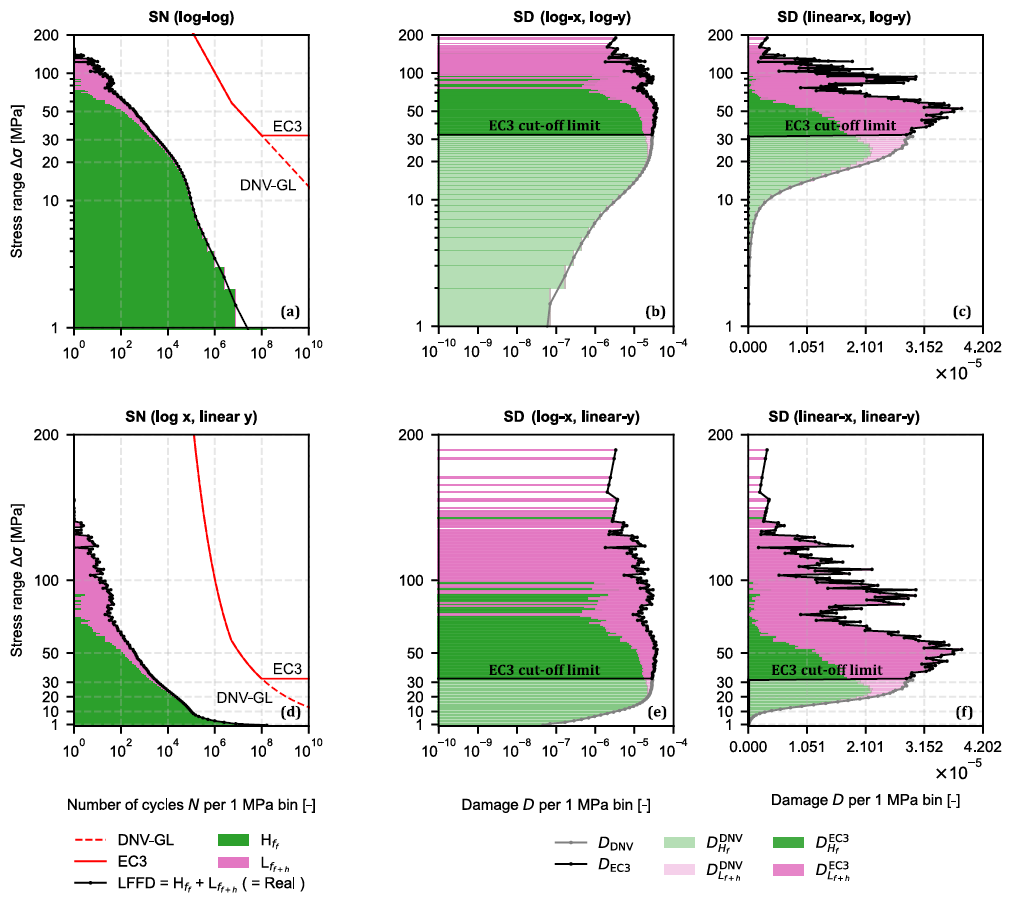
Figure 6 Comparison of Δσ−N and Δσ−D fatigue representations for conventional 10 min windows. Panels (a) and (d) show the Δσ−N distributions together with the EC3 and DNV σ−N curves. The top row (a–c) uses logarithmic scaling on the y axis, while the bottom row (d–f) uses linear scaling on the y axis. Panels (b) and (e) present the corresponding Δσ−D distributions with logarithmic scaling on the x axis, whereas panels (c) and (f) show the same distributions using linear scaling on the x axis. Green and pink denote the LFFD high-frequency and low-frequency fatigue contributions, respectively, while the black curve represents the total fatigue distribution.

Figure 6 compares different Δσ−N and Δσ−D representations for 10 min windows as an example. Figure 6a–c use logarithmic scaling on the y axis, while Fig. 6d–f use linear scaling on the y axis. Figure 6a and d show the corresponding Δσ−N histograms together with the reference EC3 and DNV σ−N curves. Figure 6b and e present the associated Δσ−D distributions using logarithmic scaling on the x axis, whereas Fig. 6c and f show the same Δσ−D distributions using linear scaling on the x axis. In all cases, the fatigue contributions are decomposed into high-frequency (green) and low-frequency (pink) low-frequency fatigue dynamics (LFFD) components, while the black curve represents the total fatigue distribution.

The comparison highlights how the choice of axis scaling influences the apparent smoothness of the fatigue distributions and the visibility of the damage-dominant stress ranges. Logarithmic scaling produces smoother Δσ−D curves and can facilitate trend identification across a broad range of stress intervals. However, it may also reduce the visibility of the relative contribution of individual stress ranges to the overall fatigue damage. In contrast, linear scaling provides a clearer representation of where damage accumulates within the spectrum and improves the identification of the dominant fatigue ranges. For this reason, the remainder of the analysis adopts linear scaling for both axes in the Δσ−D representations.

4.2 Assessment of standards in damage calculation

Eurocode 3 (EC3) provides fatigue classes explicitly linked to welded steel details typical of tubular towers, such as longitudinal and circumferential welds and attachments, enabling detail-specific fatigue assessment. In contrast, the DNVGL-RP-C203 (DNV) defines broader welded-steel fatigue classes developed for a wider range of offshore and onshore applications, which can result in different levels of conservatism when applied to tower shell structures. For lifetime-extension assessments, the choice of fatigue standard can therefore materially influence the inferred remaining life.

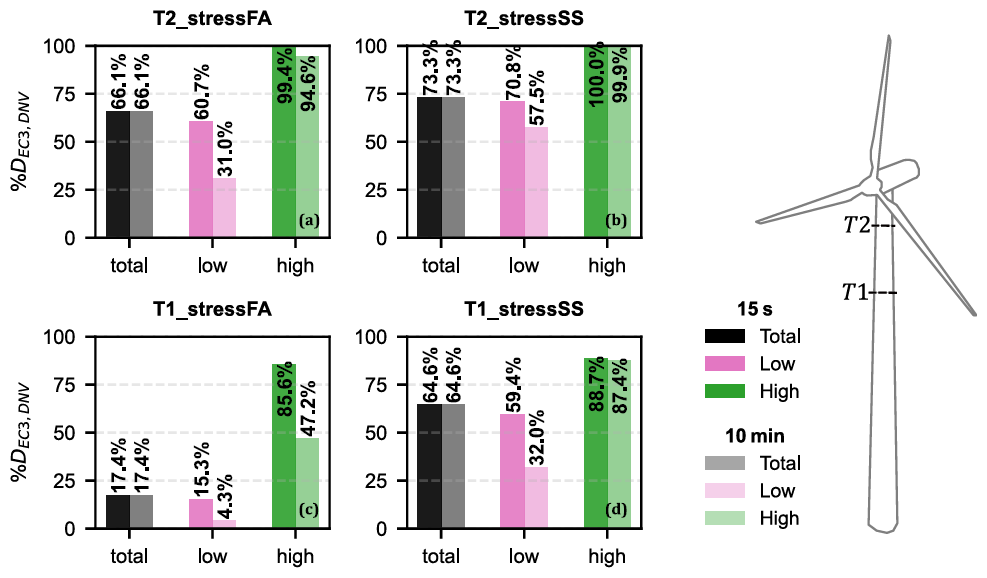
Figure 7 Relative differences between fatigue-damage estimates obtained using Eurocode 3 (EC3) and DNVGL-RP-C203 (DNV) for 10 min and 15 s windows. Damage is computed using EC3 detail category 80 and DNVGL-RP-C203 welded-steel σ−N curves, both employing a bi-linear formulation with slopes $\mathbf{m}=\mathbf{3}/\mathbf{5}$. Results are shown for tower section T1 (near-base) and T2 (upper tower) in the fore–aft (FA) and side-to-side (SS) directions: (a) T2–FA, (b) T2–SS, (c) T1–FA, (d) T1–SS. Bars indicate percentage differences in accumulated damage between EC3 and DNV for the total fatigue damage and for the low- and high-frequency contributions, computed using Eq. (3).

Figure 7 compares the relative differences between EC3- and DNV-based fatigue-damage estimates for 10 min and 15 s windows, considering both total fatigue damage and its low- and high-frequency contributions. Damage was computed using EC3 (Eurocode 3) detail category 80 and DNVGL-RP-C203 welded-steel, both using a bi-linear σ−N curve with slopes $m=\mathrm{3}/\mathrm{5}$. Because low-frequency fatigue dynamics (LFFD) preserves the total accumulated fatigue damage across windows, the relative difference between EC3- and DNV-based total damage estimates is unaffected by window length. However, changes in window length alter the partitioning between low- and high-frequency contributions, thereby altering how each fatigue standard weights the underlying stress-range distribution. For tower section T1 in the fore–aft direction, EC3 yields fatigue-damage estimates that are 17.4 % lower than those obtained using DNV for both window lengths (Fig. 7c). The reduction increases to 66.1 % at section T2, consistent with a stress-range distribution dominated by lower-amplitude cycles at higher elevations, which are weighted differently by the EC3 and DNV σ−N formulations. Comparable trends are observed in the side-to-side (SS) direction at both tower sections (Fig. 7b and d).

4.3 Influence of the data sampling rate

In the previously presented analysis, results were shown for data sampled at 50 Hz, which corresponds to the acquisition frequency of the strain measurements. Although high-frequency data are desirable for fatigue evaluation, processing long-term measurements at such high sampling rates is computationally impractical. For this reason, the 50 Hz strain signals were decimated to 25, 12.5, and 6.25 Hz. The minimum rate (6.25 Hz) was selected to remain above the dominant structural-response bandwidth observed in the measurements (most energy below ∼5 Hz). The baseline damage for sampling-rate comparisons is defined as the 50 Hz continuous rainflow result.

Sampling-rate effects were assessed for (i) the total accumulated damage and (ii) the low- and high-frequency contributions. Because total low-frequency fatigue dynamics (LFFD) damage is rainflow-equivalent, any change due to decimation reflects a loss of cycle resolution rather than windowing effects; changes in the low-frequency and high-frequency partitions are interpreted in the context of the selected window length.

Figure 8 shows cumulative damage at tower section T1 direction fore–aft (FA) for four sampling rates (50, 25, 12.5, and 6.25 Hz) and two window lengths (10 min and 15 s). Total damage and its low-frequency and high-frequency components are reported using the EC3 model, and end-of-period values are annotated with deviations relative to the 50 Hz baseline.

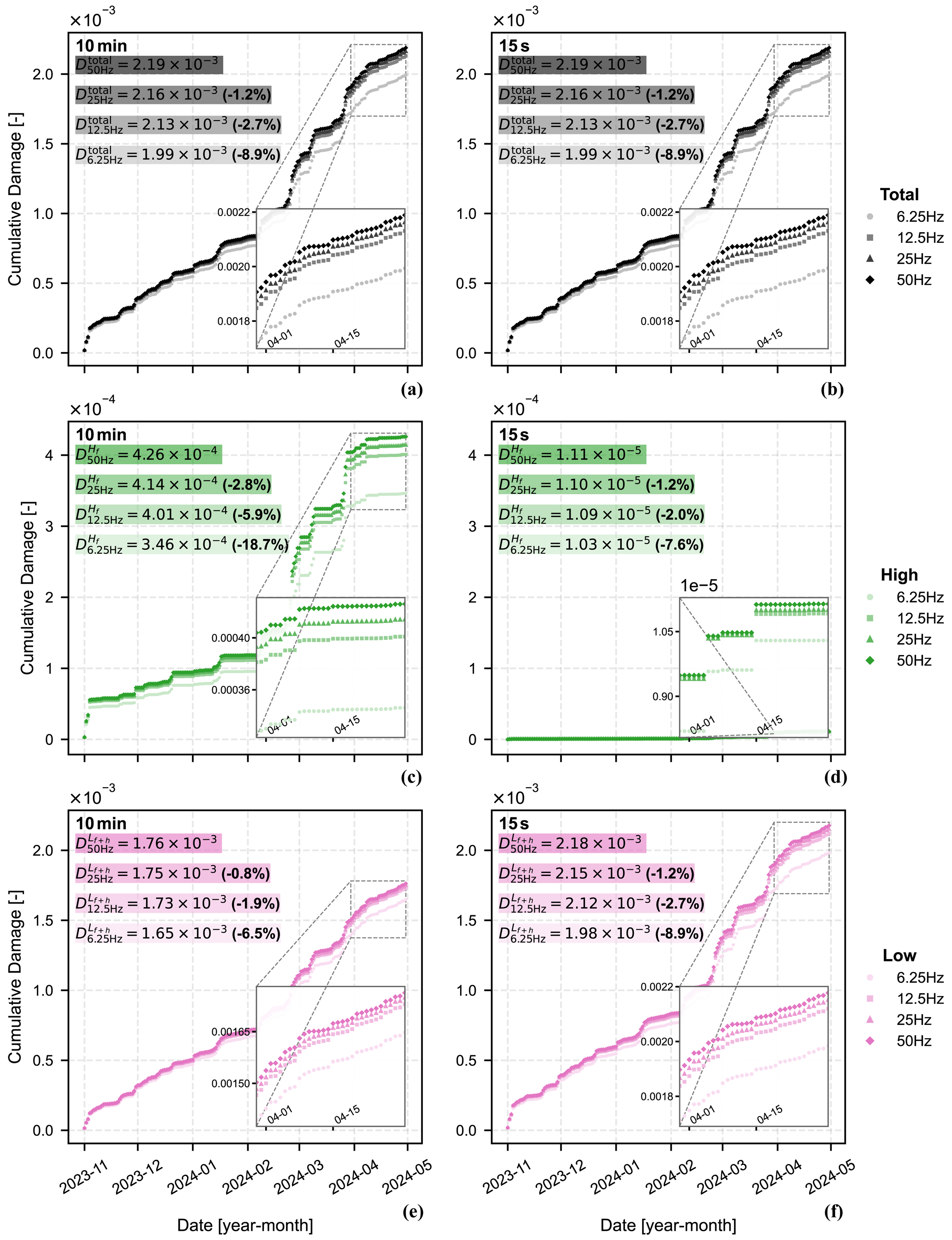
Figure 8 Cumulative FA-direction damage at tower section T1 for four sampling rates (50, 25, 12.5 and 6.25 Hz) and two window lengths, shown separately for each fatigue component: (a, b) total, (c, d) high-frequency, and (e, f) low-frequency contributions computed with EC3 detail category 80 curve. Columns (a), (c), (e) correspond to the 10 min and (b), (d), (f) to 15 s window lengths. Annotations report end-of-period values and deviations from the 50 Hz baseline, computed by Eq. (4). Insets show a close-up view of the final month of the analysis period.

Total accumulated damage decreases systematically with sampling rate, with reductions up to ∼9 % at 6.25 Hz relative to 50 Hz (Fig. 8). The close agreement at 25 and 12.5 Hz (reductions of ∼1.2 % and ∼3 %, respectively) indicates that these rates capture most fatigue-relevant content in this signal. At 6.25 Hz, damage is modestly underestimated but remains within ∼9 %.

Low-frequency damage is relatively robust to decimation. For 10 min windows, reductions remain <1 % at 25 Hz and increase to ∼6.5 % at 6.25 Hz; similar behaviour occurs for 15 s windows, with differences mainly in the low- and high-frequency partitions rather than in total damage.

High-frequency damage is more sensitive to decimation. For 10 min windows, high-frequency damage decreases substantially with sampling rate, reaching ∼ 20 % reduction at 6.25 Hz. For 15 s windows, within-window closed-cycle damage is already small because most excursions do not close within a short window; decimation further reduces the remaining within-window cycle resolution.

Figure 9 summarises the relative damage loss with respect to 50 Hz for fore–aft (FA) and side-to-side (SS) at tower section T1, for total damage and the low-frequency and high-frequency components, and for both 10 min and 15 s windows. Values are shown as 6-month means with standard deviations.

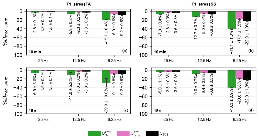
Figure 9 Relative damage loss with respect to 50 Hz at tower section T1 for fore–aft (FA) and side-to-side (SS), computed by Eq. (4). Bars show total, low-frequency, and high-frequency contributions for 25, 12.5, and 6.25 Hz, using 10 min and 15 s windows. Values are 6-month means with standard deviations. Damage computed with EC3 detail category 80 curve.

Across both directions and window lengths, total damage loss increases as sampling rate decreases (Fig. 9). At 25 Hz and 12.5 Hz, total losses are typically below ∼3.6 %, while at 6.25 Hz losses increase to ∼9 % in fore–aft (FA) and exceed ∼20 % in side-to-side (SS), indicating higher sensitivity of the SS response to undersampling. This is consistent with the different loading mechanisms governing each direction: FA is dominated by aerodynamic thrust, which varies with wind speed and produces larger-amplitude stress excursions driven by comparatively slow, longer-duration variations, whereas SS is dominated by rotor torque and rotational loading linked to blade-passing frequency, producing smaller-amplitude, shorter-duration cycles that are more susceptible to loss under decimation. This is reflected in the substantially larger total FA damage and its wider stress-range spectrum (Fig. 10), and in the SS direction's greater sensitivity to decimation in both the high- and low-frequency components at 6.25 Hz, for both window lengths (10 min: −17.1 % vs. −6.9 %; 15 s: −20.8 % vs. −9.1 %, for the low-frequency component alone), indicating that shorter-duration rotor-rotational content is present throughout the SS signal rather than confined to intra-window cycles. This directional sensitivity is not universal: at tower section T2, FA shows greater sensitivity, consistent with that section's proximity to the nacelle and its associated drivetrain/rotor excitations.

The low-frequency component shows moderate and consistent sensitivity, remaining below ∼10 % loss in fore–aft (FA) and below ∼ 21 % in side-to-side (SS) at 6.25 Hz. In contrast, the high-frequency component is substantially more sensitive, particularly for 10 min windows, where losses can reach ∼20 %–40 % at 6.25 Hz depending on direction.

Although sampling rates of 25 and 12.5 Hz provide closer agreement with the 50 Hz baseline, the 6.25 Hz case is retained in the subsequent analysis as a deliberately conservative lower-resolution scenario. The objective is not to identify an optimal sampling rate but to evaluate the robustness of the proposed fatigue-monitoring strategies under restrictive temporal resolution and computational constraints. The use of 6.25 Hz, therefore, represents a lower-bound scenario in which the resulting bias in total fatigue damage remains bounded and explicitly quantified for the present dataset. While the magnitude of this bias is inherently case-dependent and may vary across turbine configurations and response characteristics, adopting the lowest admissible sampling rate provides a stringent, transparent basis for benchmarking reduced-information fatigue-monitoring approaches under realistic large-scale deployment conditions.

4.4 Influence of window length

To isolate the influence of window length on fatigue characterisation without conflating it with information loss, the analysis first considers window-length effects within the residual-preserving low-frequency fatigue dynamics (LFFD) framework. This enables assessment of the effect of window segmentation itself, before introducing additional approximations associated with reduced-information representations.

The selection of the window directly influences how stress excursions are classified between within-window full cycles and residual-based cycles spanning adjacent windows in the low-frequency fatigue dynamics (LFFD) framework. Reducing the window length increases the likelihood that slowly varying stress excursions remain unclosed within an individual window and are therefore transferred to the residual sequence. Consequently, although the total fatigue damage remains theoretically equivalent to continuous rainflow counting, the relative contribution of the identified high- and low-frequency fatigue components may change significantly with the adopted window duration.

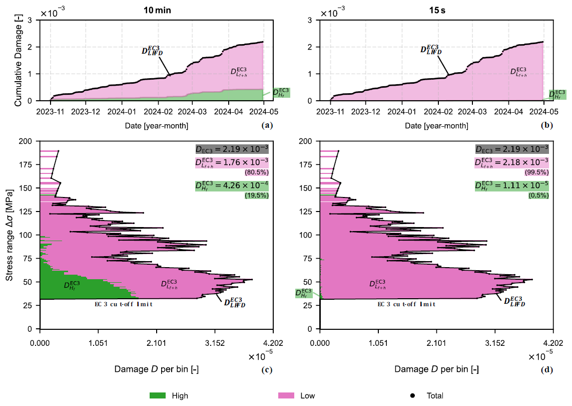
Figure 10 FA-direction fatigue at tower section T1 (6 months, 50 Hz), computed using the EC3 detail category 80 σ−N curve (bi-linear formulation, slopes $m=\mathrm{3}/\mathrm{5}$). (a–b) Cumulative damage for 10 min and 15 s windows. (c–d) Final Δσ−D spectra. Total damage is decomposed into within-window full-cycle damage (green) and residual-based damage (pink). The percentages of damage are computed by Eq. (2).

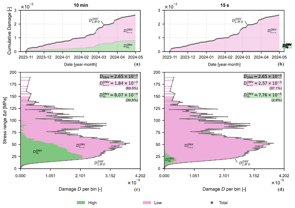
Figure 11 FA-direction fatigue at tower section T1 (6 months, 50 Hz), computed using the DNV welded-steel σ−N curve (bi-linear formulation, slopes $m=\mathrm{3}/\mathrm{5}$). (a–b) Cumulative damage for 10 min and 15 s windows. (c–d) Final Δσ−D spectra. Total damage is decomposed into within-window full-cycle damage (green) and residual-based damage (pink). The percentages of damage are computed by Eq. (2).

Figures 10 and 11 present the fatigue response in the fore–aft (FA) direction at tower section T1, which exhibits the highest accumulated fatigue damage. Results are shown for 50 Hz strain data aggregated using 10 min and 15 s windows. Panels (a)–(b) show cumulative damage, and panels (c)–(d) show the final Δσ−D spectra. Total damage (black/grey) is decomposed into within-window high-frequency full-cycle damage (green) and low-frequency full- and half-cycle damage spanning windows (pink) and is computed using both EC3 and DNV.

As shown in Figs. 10 and 11, the total fatigue damage obtained with low-frequency fatigue dynamics (LFFD) is independent of window length, because the method preserves rainflow equivalence through the combination of within-window full cycles and the concatenated residual sequence. The absolute damage level depends on the adopted σ−N curve; this effect is discussed in Sect. 4.2. In contrast to the total damage, the partition between low- and high-frequency contributions changes markedly with window length.

For EC3, the low-frequency damage increases from $\mathrm{1.76}\times {\mathrm{10}}^{-\mathrm{3}}$ (80.5 % of total) for 10 min windows to $\mathrm{2.18}\times {\mathrm{10}}^{-\mathrm{3}}$ (99.5 % of total) for 15 s windows, i.e. a 19 % increase in the low-frequency contribution when the window is reduced from 10 min to 15 s (Fig. 10). This shift is a direct consequence of signal segmentation: shorter windows increase the probability that stress excursions are truncated at window boundaries and, as a result, reconstructed through the residual sequence. With 15 s windows, many stress excursions driven by slowly varying mean loads and operational transitions do not fully close within a single window and are therefore carried into the residual sequence and recovered by residual concatenation. The increase in the low-frequency contribution is thus a redistribution of identified cycles caused by segmentation, rather than a physical increase in low-frequency loading.

This link between operational-state transitions and the low-frequency damage contribution motivates a more detailed characterisation of individual states (e.g. start-up, shutdown, idling). However, the analysed period is dominated by steady production states (Run: 87.24 %; Ready: 11.49 %; Sect. 3), with transient states occurring comparatively rarely; a statistically robust, per-state decomposition of fatigue damage was therefore not pursued in this study and would require a longer monitoring dataset. It is identified as a valuable direction for future work (Sect. 5).

For 15 s windows, most fatigue damage is recovered through the residual sequence because short windows reduce the likelihood of stress excursions closing within a single window. Consequently, the suitability of a 15 s window depends on the dominant frequency content of the structural stress response relative to the selected window length, rather than representing a universally optimal choice.

The same trend is observed with the DNV damage model (Fig. 11), although the change is larger: for 15 s windows, the low-frequency contribution reaches 97.1 % of the total, corresponding to a 27.6 % increase relative to 10 min windows.

4.5 Comparison of fatigue monitoring methods

Having established the influence of window length within a rainflow-equivalent framework, the analysis now turns to reduced-information and window-based methods. Unlike low-frequency fatigue dynamics (LFFD), these approaches introduce varying degrees of approximation, such that their accuracy reflects both their inherent representation strategy and its interaction with the chosen window length – shorter windows increase reliance on extrema preservation, while longer windows favour within-window cycle closure at the expense of long-period dynamics. Each method is benchmarked against the low-frequency fatigue dynamics (LFFD) baseline across both window lengths.

To evaluate the combined influence of window length and information reduction on fatigue estimation, four monitoring approaches are compared. These include (i) the residual-preserving low-frequency fatigue dynamics (LFFD) methodology, which preserves rainflow equivalence and is adopted as the baseline (Faria et al., 2024; Marsh, 2016; Marsh et al., 2016; Sadeghi et al., 2022, 2023; Shah et al., 2025, 2026); (ii) conventional window-based high cycle rainflow counting using fixed window lengths in accordance with IEC practice (IEC 61400-13, 2015); and (iii) two reduced information extrema sequence representations, namely the start–peaks–valleys–end (SPVE) and maximum–minimum (max–min) methods, which retain only representative stress extrema per window to reduce computational and storage demands (Larsen and Thomsen, 1996; Shah et al., 2025, 2026). These methods span the range from rainflow-equivalent fatigue estimation to highly compressed representations, enabling systematic assessment of how window length interacts with different levels of information reduction.

Figures 12 and 13 present cumulative damage and end-of-period Δσ−N and Δσ−D spectra for all methods. Differences are most pronounced under 10 min windowing, where segmentation truncates long-period stress variations and suppresses moderate stress-range content that contributes materially to damage accumulation. The start–peaks–valleys–end (SPVE) sequence reproduces fatigue-damage levels very close to the low-frequency fatigue dynamics (LFFD) baseline for both window lengths, demonstrating that preserving a limited set of representative turning points per window is sufficient to retain most fatigue-relevant information without requiring within-window rainflow counting. In contrast, the max–min approach exhibits a strong dependence on window length: under 10 min windowing, it substantially underestimates fatigue damage due to the loss of moderate-stress-range cycles, whereas for 15 s windows, its agreement with the baseline improves markedly as extrema more accurately represent the underlying turning-point sequence (Fig. 13).

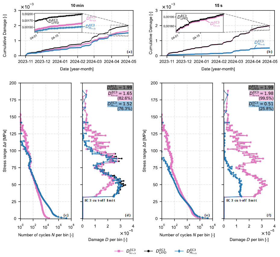
Figure 12 FA-direction fatigue at tower section T1 (6 months, 6.25 Hz): residual-preserving LFFD versus conventional window-based counting. (a–b) Cumulative damage for 10 min and 15 s windows. (c, e) Δσ−N spectra and (d, f) Δσ−D spectra at the end of the 6 months, for 10 min and 15 s windows respectively. Curves compare LFFD total damage (baseline), the LFFD low-frequency contribution, and conventional window-based high-cycle counting. Percentages indicate damage relative to the LFFD baseline (Eq. 5, EC3). Insets show a close-up view of the final month of the monitoring period (15 s panel restricted to LFFD total and low-frequency, for clarity). Damage is computed using EC3 detail category 80, employing a bi-linear formulation with slopes $m=\mathrm{3}/\mathrm{5}$.

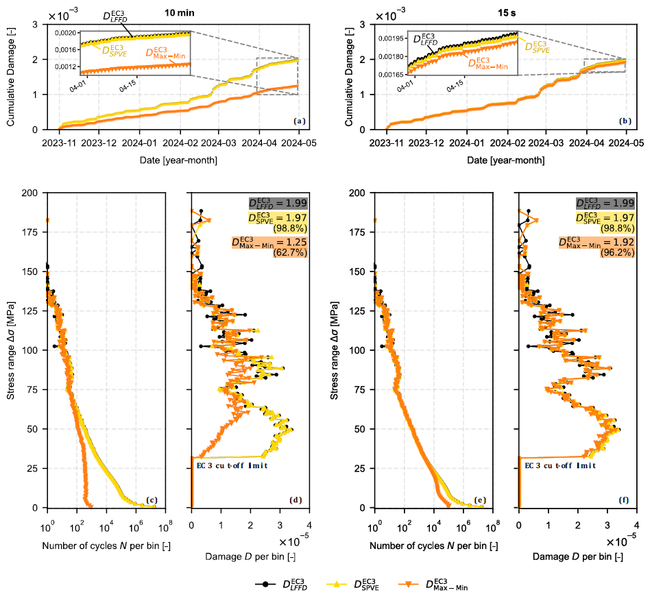
Figure 13 FA-direction fatigue at tower section T1 (6 months, 6.25 Hz): LFFD baseline versus reduced-information extrema representations. (a–b) Cumulative damage for 10 min and 15 s windows. (c, e) Δσ−N spectra and (d, f) Δσ−D spectra at the end of the 6 months, for 10 min and 15 s windows respectively. Curves compare LFFD total damage (baseline), start–peaks–valleys–end (SPVE), and maximum–minimum (max–min). Percentages indicate damage relative to the LFFD baseline (Eq. 5, EC3). Insets show a close-up view of the final month of the monitoring period. Damage is computed using EC3 detail category 80, employing a bi-linear formulation with slopes $m=\mathrm{3}/\mathrm{5}$.

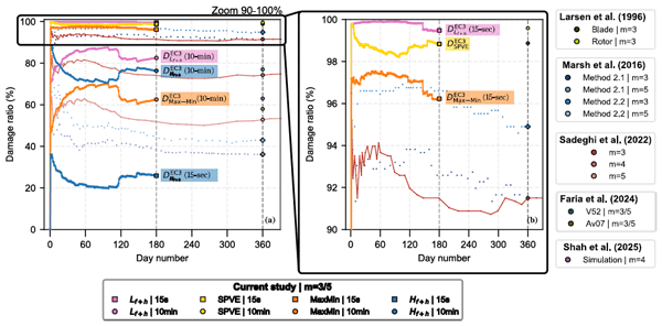
Figure 14 summarises the accuracy of each fatigue monitoring methodology using the damage ratio defined in Eq. (5) as a function of window length, and Table 2 places these results in the context of representative literature findings for different fatigue exponents and turbine components. Figure 14a–b compare the performance of the evaluated methods under 10 min and 15 s windows. High-fidelity fatigue assessment can be achieved using highly compressed stress representations, particularly when short window lengths are adopted. For 15 s windows, both residual-preserving and extrema-based approaches achieve damage ratios close to unity, whereas larger deviations are observed under conventional 10 min windows due to truncation of long-period stress variations.

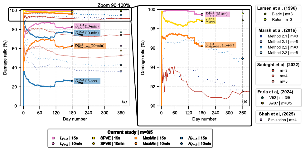
Figure 14 Fatigue-damage accuracy as a function of window length, expressed through the damage ratio defined in Eq. (5). Values close to 100 % indicate agreement with the baseline, while deviations quantify under- or over-estimation due to aggregation and information reduction. Panels (a) and (b) show damage ratios obtained in the present study for 10 min and 15 s windows respectively, comparing LFFD, start–peaks–valleys–end (SPVE), max–min, and conventional window-based high cycle counting.

Table 2 Comparison of fatigue-damage ratios (%) reported in the literature and obtained in the present study for different damage estimation methods, window lengths, and fatigue slopes (m) (Faria et al., 2024; Larsen and Thomsen, 1996; Marsh, 2016; Marsh et al., 2016; Sadeghi et al., 2022; Shah et al., 2025). For the current study, values represent the ratio of estimated damage to the continuous rainflow counting baseline defined in Eq. (5). For literature studies, values represent the ratio of damage estimated without low-frequency fatigue cycle recovery to the damage estimated with full residual concatenation. Results cover a range of turbine components, modelling approaches, and damage accumulation strategies, providing a benchmark for evaluating the performance of the proposed methods.

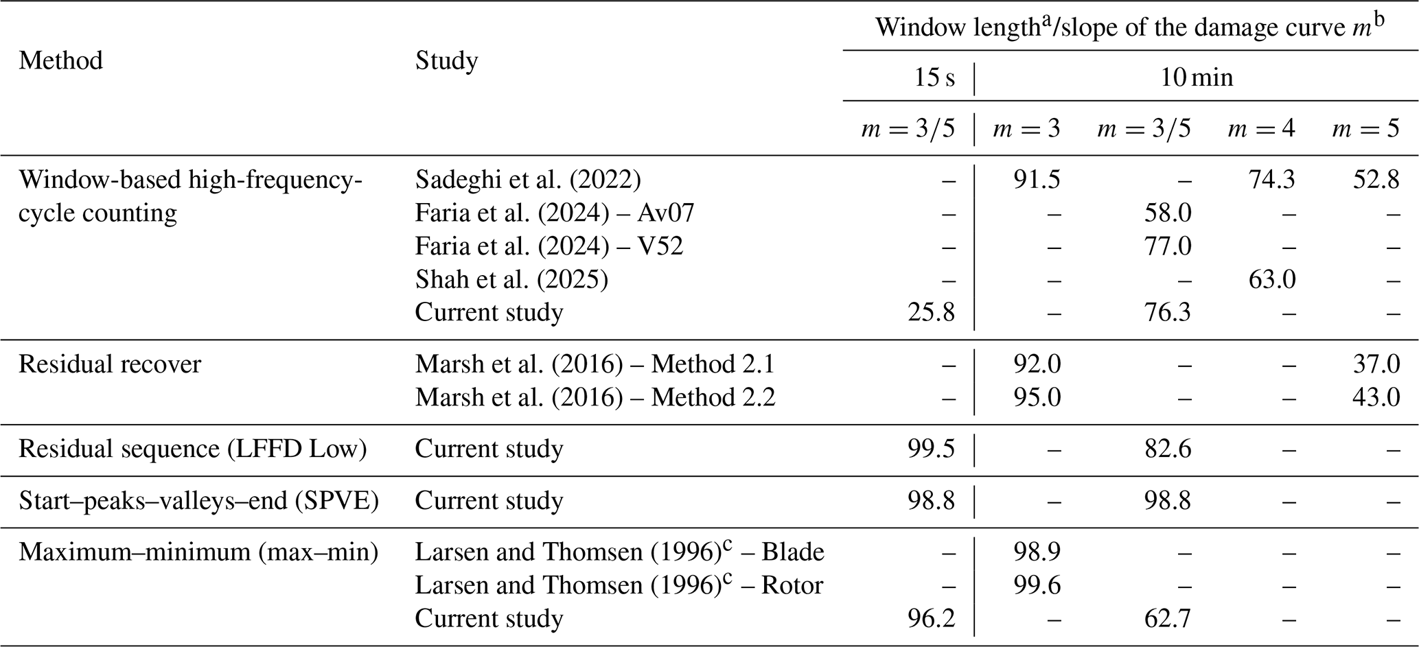
^a All literature values correspond to 10 min window lengths unless otherwise indicated. ^b The $m=\mathrm{3}/\mathrm{5}$ column refers to a bi-linear σ−N curve formulation with slopes m=3 and m=5, as used in Eurocode 3 and DNV standards. Single-slope results from the literature (m=3, m=4, m=5) are reported in the respective columns. ^c Larsen and Thomsen (1996) values represent the high-frequency damage contribution prior to inclusion of the low-frequency component, applied to blade flapwise and rotor tilt moments using a max–min approximation.

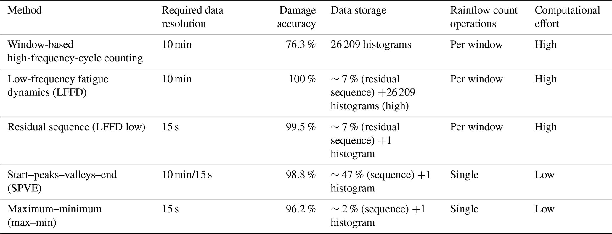
Practical deployment at wind-farm scale is constrained not only by estimation accuracy but also by data-handling and computational requirements. To assess these aspects, each methodology was evaluated using only the data strictly required for its implementation. Retaining only the concatenated residual sequence within the low-frequency fatigue dynamics (LFFD) framework requires approximately 7 % of the raw data volume, while the maximum–minimum (max–min) representation reduces this further to about 2 %, and start–peaks–valleys–end (SPVE) retains roughly 50 %. Extrema-based representations further reduce computational complexity by requiring only a single rainflow counting operation on the concatenated reduced sequence, rather than repeated cycle counting at every window. For 15 s windows, start–peaks–valleys–end (SPVE) achieves approximately 99 % damage accuracy with around 50 % data reduction, while maximum–minimum (max–min) reaches roughly 96 % accuracy while retaining only about 2 % of the original data.

The evaluated methodologies are summarised in Table 3 according to required data resolution, damage accuracy, computational effort, and storage requirements. Taken together, these results demonstrate that accurate fatigue estimation can be achieved using highly reduced stress representations when short, SCADA-aligned windows are adopted. Residual-preserving and extrema-based approaches retain the fatigue-relevant information required for rainflow-equivalent damage estimation, while substantially reducing data volume and computational complexity, enabling practical implementation of fatigue monitoring at sub-minute resolution using operational SCADA and strain measurements, without requiring continuous high-frequency data storage or processing.

Table 3 Overview of the fatigue assessment methods evaluated in this study, summarising data resolution requirements, computational effort, storage needs, and the comparative characteristics of each method. Computational effort refers to the need to perform rainflow cycle counting repeatedly at the window level versus a single rainflow operation applied to a concatenated reduced information stress sequence. All percentages are expressed relative to the raw 50 Hz signal length (Eq. 6). A single histogram is negligible in storage terms relative to the raw signal length; window-based approaches (rows 1–2) instead require one histogram per 10 min window, giving ∼ 26 209 histograms over the 6-month record.

The fatigue-damage estimates presented above relate specifically to the instrumented tower sections, T1 and T2. Extrapolating these estimates to other locations of practical interest, such as the tower base or tower top, is a distinct problem from the reconstruction addressed here: it cannot be validated directly against measurements at those locations and instead requires an explicit load-transfer relationship, for example derived from a structural/modal model or from a data-driven prediction approach, established between the instrumented sections and the location of interest. Differences in local dynamic response, modal contributions, and load-path characteristics along the tower height mean that such a relationship cannot be assumed to hold without dedicated validation.

5 Conclusions

This study assessed fatigue-monitoring methodologies suitable for real-time fleet-scale deployment on wind turbines, using 6 months of high-frequency tower-strain measurements from an onshore turbine. Rainflow cycle counting (RFC) was used as the baseline, against which window-based approaches, the low-frequency fatigue dynamics (LFFD) method, and two reduced-information extrema-sequence representations, start–peaks–valleys–end (SPVE) and maximum–minimum (max–min), were benchmarked across multiple sampling rates, window lengths, and two fatigue-curve standards (Eurocode 3 and DNV).

The central question addressed is whether SCADA-aligned short windows can replace the conventional 10 min standard while preserving fatigue-damage accuracy and remaining practically deployable at scale. The results show that the answer depends critically on the method used. Conventional 10 min window-based counting recovered only 76.3 % of baseline damage due to cycle truncation at boundaries. Reducing the window length to 15 s does not resolve this – shorter windows increasingly truncate the low-frequency cycles that dominate fatigue damage, and the window-based method retains only 25.8 % of baseline damage at 15 s segmentation. It is the low-frequency fatigue dynamics (LFFD) formulation that removes this window-length dependence entirely: by explicitly reconstructing inter-window cycles through residual concatenation, it recovers 99.5 % of baseline damage regardless of segmentation length. A direct consequence of 15 s segmentation is that nearly all fatigue-relevant information migrates to the inter-window residuals, with the low-frequency component accounting for 99.5 % of total damage – a redistribution driven by segmentation, not by a physical increase in low-frequency loading.

Among reduced-information methods, start–peaks–valleys–end (SPVE) reproduces 98.8 % of baseline damage across both window lengths while reducing stored data by approximately 50 % and requires only a single rainflow counting operation, making it well-suited for fleet-level fatigue monitoring. The maximum–minimum (max–min) method achieves 96.2 % accuracy at 15 s windows while retaining only ∼2 % of the raw data, the highest compression among all methods evaluated; however, its accuracy degrades substantially under 10 min windowing (62.7 %), where moderate stress-range cycles are lost. The choice between these two methods, therefore, depends on the deployment context: the start–peaks–valleys–end (SPVE) method is preferable when accuracy is the priority, while the maximum–minimum (max–min) method is better suited to highly resource-constrained architectures where extreme data compression is required.

Regarding fatigue-curve selection, EC3 estimates 17 %–66 % less accumulated damage than DNV, depending on the tower section, and is identified as the more appropriate standard for the welded tubular steel details of onshore towers. Downsampling from 50 to 12.5–25 Hz introduces negligible deviation; 6.25 Hz offered a practical compromise for scalable architectures with bounded underestimation of up to ∼9 %.

The original contributions of this work are 3-fold. First, it provides a systematic comparison of window-based, residual-preserving, and extrema-sequence fatigue-monitoring methods under SCADA-aligned short windows, using real strain data. Second, it demonstrates quantitatively that 15 s SCADA-aligned segmentation, combined with either residual-preserving processing or extrema sequences, enables accurate and data-efficient fatigue monitoring without continuous high-frequency data storage. Third, it establishes that the inter-window residual sequence alone, at only ∼ 7 % of the raw data volume, is sufficient to reconstruct reference-equivalent fatigue damage, offering a practical pathway for long-term fleet-scale monitoring.

The reduced-information representations evaluated here were designed and assessed specifically for fatigue-damage estimation; their suitability for other SHM applications, such as frequency-domain analyses (FFT, PSD) for modal identification or vibration-based damage detection, strain-gauge calibration checks, or virtual-sensing algorithms, falls outside the scope of this study and remains an open question for future work. Future work will apply the proposed 15 s SCADA-aligned fatigue estimation framework to long-term operational data and will explore fatigue prediction at the finest achievable granularity by forecasting extrema sequences, particularly maximum–minimum (max–min) representations at 15 s resolution, and by predicting the low-frequency residual sequence directly, which this study shows accounts for the large majority of fatigue damage at short window lengths while representing only ∼7 % of the raw data volume. This approach aims to enable predictive fatigue monitoring without requiring continuous high-frequency strain measurements, supporting proactive lifetime management at wind-farm scale. Further valuable directions for future work include the following: a direction-resolved analysis of turbulence and possible wake effects on tower fatigue, requiring simultaneous strain measurements from multiple turbines across the array; extrapolation of fatigue-damage estimates from the instrumented tower sections to other locations of interest, such as the tower base or tower top, through validated load-transfer or data-driven relationships; and a quantitative decomposition of fatigue damage by operational state, isolating the contribution of start-up, shutdown, and idling transients from steady production.

Appendix A: List of abbreviations

EC3	Eurocode 3 design standard for steel structures
DNV	DNVGL-RP-C203 recommended practice for fatigue design of offshore and onshore steel structures
FA	Fore–aft direction of the wind turbine tower
HF	High-frequency fatigue contribution (cycles closing within a window)
LFFD	Low-frequency fatigue dynamics methodology
LF	Low-frequency fatigue contribution (cycles spanning multiple windows and reconstructed via residuals)
Max–min	Maximum–minimum extrema sequence representation
RFC	Rainflow cycle counting
SCADA	Supervisory control and data acquisition
SHM	Structural health monitoring
SPVE	Start–peaks–valleys–end extrema sequence representation
SS	Side-to-side direction of the wind turbine tower