
the Creative Commons Attribution 4.0 License.
the Creative Commons Attribution 4.0 License.
 | 15 Oct 2026
A multi-stage methodology for wind park inter-array cabling: graph preparation, routing, and sizing
Bernardo Castro Valerio

Pieter M. O. Gebraad
Marc Cheah-Mane
Vinicius A. Lacerda
Oriol Gomis-Bellmunt
Inter-array grid optimisation plays a critical role in the technical and economic performance of wind parks and is typically divided into two primary tasks: routing length minimisation and conductor size selection. This work proposes the consideration of three primary tasks, beginning with graph preparation to account for terrain profiles, soft- and hard-exclusion zones, and export cables. Once a graph with viable connection pathways is established, a routing mixed-integer linear formulation for radial arrays, subject to crossing constraints and a maximum number of turbines per string, is presented. This formulation can be adapted to user requirements to include a minimum number of turbines per string, as well as a methodology to determine the minimum number of substation connections required under irregular turbine distributions arising from terrain constraints. Conductor size selection is addressed through a linear approximation of the power flow, enabling the limitation of the number of conductor types used within the system. Routing and conductor size selection may be combined within an integrated approach or implemented as a sequential algorithm to explore trade-offs between trenching and cabling costs. The proposed approaches are evaluated using current turbine ratings and the cable routings of existing onshore and offshore projects. The integrated formulation generally achieves lower total costs, while the sequential approach offers greater modelling flexibility for constrained routing problems. The results further demonstrate that routings with minimum trench length do not necessarily minimise total investment cost, since limiting the number of conductor types may exclude larger conductor capacities, thereby changing the feasible routing configurations and the conductor types ultimately selected within the system.
- Article
(7440 KB) - Full-text XML
- BibTeX
- EndNote


Wind energy has become a central component of the global energy transition. In wind park design, once turbine locations have been determined through wind resource and wake optimisation, attention shifts to the inter-array cable system, which interconnects turbines and transmits power to substations. The configuration of this electrical collection network is shaped by routing complexity arising from terrain conditions, spatial constraints, and installation limitations. Optimising this configuration is highly relevant for cost-effectiveness; for example, in bottom-fixed offshore wind farms, inter-array cables may account for up to approximately 8 %–9 % of the levelised cost of energy (LCoE) (Serrano González et al., 2014; BGV Associates, 2025). The design of the cable array constitutes a critical aspect of the overall wind park configuration. This process may be divided into two primary tasks: first, collector-system optimisation to minimise cable lengths; second, conductor size selection (CSS).
Before optimising the connections between turbines, real-world site constraints must be translated into a mathematical graph model. Many studies construct a two-dimensional graph using Euclidean distances between candidate connection points. A notable exception is Gong et al. (2018), which applies a geodesic algorithm on a three-dimensional seabed to calculate connection distances, although it does not include Geographic Information System (GIS) constraints. As offshore sites become more spatially constrained, several formulations have introduced Steiner nodes to model detours around exclusion zones (Fischetti and Pisinger, 2018a, b; Taylor et al., 2023b). Penalty-based treatments of spatial restrictions have also been used in complex offshore routing studies; for example, Taylor et al. (2023b) penalise crossings of wind-farm boundaries and obstacle regions while using Steiner nodes to support obstacle navigation. More detailed spatial-preprocessing approaches include Delaunay triangulation-based navigational mesh pathfinding (Pillai et al., 2015) and topology-embedding separation with post-optimisation detours for non-straight cable routes (Souza de Alencar et al., 2025). These approaches primarily address obstacle avoidance, penalised spatial violations, or feasible route construction, while the distinction between prohibited regions and feasible but undesirable routing areas is less commonly treated explicitly at the graph-construction stage, particularly when final cable routes are embedded only after topology optimisation.
Once the candidate graph has been defined, the routing formulation determines which connections are installed and which topological restrictions are enforced. In the collector-system optimisation phase, multiple topologies have been implemented in practice, including radial, radial plus star, radial plus star with splices, single loop, and others (Pérez-Rúa and Cutululis, 2019). In the present work, radial arrays are interpreted as string-like routings in which turbine–node bifurcations are not permitted. To address collector-system optimisation, various approaches have been employed, including graph-based methods derived from the minimum spanning tree (MST) and travelling salesman problem (TSP) formulations (Dutta and Overbye, 2012; Wei et al., 2017), ant colony optimisation (Taylor et al., 2023a), mixed-integer linear programming (MILP) (Fischetti and Pisinger, 2018a, b; Pillai et al., 2015; Pérez-Rúa et al., 2020a; Ulku and Alabas-Uslu, 2020; Souza de Alencar et al., 2025), and heuristic approaches (Cazzaro et al., 2020; El Mokhi and Addaim, 2020; Sedighi et al., 2018; Gong et al., 2018), including genetic algorithms (Moon et al., 2014; Wei et al., 2017; Smail et al., 2018) and particle swarm optimisation (Hou et al., 2016). In this context, a balanced configuration refers to limiting disparities in the number of turbines connected per substation and per string, thereby resulting in advantages in installation planning and transformer specification, as discussed in Cazzaro and Pisinger (2022).
Existing routing formulations address these topological and spatial restrictions in different ways. Several MILP formulations represent candidate connections using directed arc-pairs, so that the selected direction follows the energy flow towards the substation rather than being fixed by geometry (Fischetti and Pisinger, 2018a, b; Pérez-Rúa et al., 2020a). Other approaches introduce iterative crossing constraints, practical topology variants, or topology-embedding separation to obtain feasible cable routes (Pillai et al., 2015; Fischetti and Pisinger, 2018b; Souza de Alencar et al., 2025). These studies demonstrate that routing constraints such as crossings, substation limits, conductor capacities, branching, and string structures have been widely considered. However, fewer studies explicitly consider how spatially feasible candidate connections should be constructed when strict string-like radial topologies, practical balancing constraints, and clearance requirements around fixed structures must be satisfied simultaneously.
Beyond the selection of cable routes, conductor sizes must be chosen to satisfy current limits while balancing investment and loss-related costs. This can be achieved either through static rated sizing, which assumes a continuous current over time, or through a dynamic load cycle profile, which accounts for the variability in power production (Pérez-Rúa and Cutululis, 2019). To address the CSS problem, studies have employed genetic algorithms (Smail et al., 2018; Rentschler et al., 2019), modified bat algorithms (Qi et al., 2019), and MILP formulations (Wędzik et al., 2016; Chen et al., 2016; Fischetti and Pisinger, 2018a; Pérez-Rúa et al., 2020a). Loss-aware cable selection has also been incorporated into routing and collection-system formulations through infrastructure and loss-related cost terms. For example, Cerveira et al. (2016) represent conductors using a short-line model and use precomputed loss terms within an integer linear programming formulation that minimises infrastructure and loss-related costs. Other formulations similarly use precomputed cable-cost coefficients or load-dependent loss approximations (Fischetti and Pisinger, 2018a; Pérez-Rúa et al., 2020b, a; Bae et al., 2023).
Several studies have also coupled conductor sizing with the routing or interconnection problem. For simultaneous interconnection configuration and conductor sizing, Sedighi et al. (2018) employs a harmony search algorithm for partial conductor sizing, whereby each branch along a route is assigned a conductor based on the ampacity of the final segment before it joins another route or connects to the substation. The study considers branches originating from bifurcation points; under that partial-sizing assumption the same conductor type is assigned to all sections of a string. Wędzik et al. (2016) combine network routing optimisation with CSS and include constraints on the number of cable cross-sections used for a single substation. In Pérez-Rúa et al. (2020a), an integrated routing algorithm is proposed that can adapt to multiple substations and limit static crossings; however, when considering CSS, the method does not limit the number of permitted conductors. Due to the cost associated with cable-laying vessel operations, the number of different conductor diameters used in offshore wind farm design is typically limited.
Because routing, conductor sizing, and loss representation are strongly coupled, other studies have used decomposition or hierarchical strategies to improve tractability. Benders-based formulations and decomposition-based heuristics have been proposed for collector-system planning and complex offshore routing. In Chen et al. (2016), the master problem handles cable-routing decisions while operational subproblems evaluate network feasibility. Similarly, Lumbreras and Ramos (2013) apply decomposition strategies to offshore wind farm electrical-system planning, separating investment decisions from operational scenarios and reliability-related constraints. In contrast, Taylor et al. (2023b) use a decomposition-based ant colony optimisation heuristic in which selected strings are removed and re-optimised as subproblems while the remainder of the routing is fixed. However, less attention has been given to how CSS restrictions alter the routing problem itself under spatially constrained and balanced radial-array requirements. When conductor costs scale superlinearly with power capacity and only a limited number of conductor cross-sections can be used, the shortest feasible route is not necessarily the least-cost route.
This work builds on Valerio et al. (2026b), which presents the graph preparation methodology and the mixed-integer linear formulation for routing of inter-array connections. In addition, this paper presents two methods for joint routing and conductor size optimisation. The first is an integrated approach that incorporates conductor size selection directly into the routing algorithm. The second is a sequential solution that iterates between routing and CSS, addressing a more constrained problem. Following Hou et al. (2019); Kallinger et al. (2023) and the revised literature, an algorithm designed to address the inter-array cabling of wind turbines should satisfy the following criteria.
- C1.
Consider nonhomogeneous terrain conditions.
- C2.
Avoid cable crossings in the cable routing.
- C3.
Ensure that the current in each cable under full-load conditions does not exceed its rated capacity.
- C4.
For a radial array, no bifurcations are allowed in turbine nodes.
- C5.
Limit the number of different conductor type sections.
- C6.
Aim to reduce computational cost.
To address these criteria, the main contribution of this work is a graph-prepared optimisation framework for radial inter-array grids that evaluates how spatial feasibility constraints and conductor-size restrictions jointly affect routing decisions, showing that the shortest routing solution is not necessarily the least-cost solution when CSS and conductor-type limits are considered. This contribution is supported by the following components.
-
A graph construction methodology that incorporates three-dimensional terrain, inclination constraints, and both hard- and soft-exclusion zones into the candidate edge generation process
-
A reduced MILP formulation for inter-array routing using a single binary variable per arc, providing a simplified representation of the routing decisions that can be extended with additional routing and CSS constraints
-
A joint treatment of routing and conductor size selection, in which restricting the conductor types selected from the allowable set influences the feasible routing configuration through the maximum transferable power and corresponding number of turbines per string, rather than being treated only as post-processing
-
The development and comparison of integrated and sequential approaches for joint routing and CSS, highlighting trade-offs between solution quality, modelling flexibility, and computational complexity
The final solution includes a graph preparation phase that incorporates exclusion zones and elevation into the identification of the connection process (Sect. 2). The routing algorithm is presented in Sect. 3.1, with additional modelling options described in Sect. 3.2, including constraints on the minimum number of turbines per string, the determination of substation connections, and unbalanced substation capacities. A stand-alone CSS formulation is introduced in Sect. 4. Joint routing and conductor size optimisation are then addressed through an integrated formulation (Sect. 5.1) and a sequential algorithm (Sect. 5.2). The approaches are evaluated in Sect. 6, with the results discussed in Sect. 7.
Graphs are commonly constructed using geometric two-dimensional distances between turbines. However, the quality of the optimisation strongly depends on the granularity and realism of the input data. To make the cable routing problem more accurate, it is necessary to incorporate additional spatial constraints, including bathymetry, inclination, and exclusion zones. Figure 1 illustrates the procedure for generating viable graph edges. The process integrates bathymetric or elevation data, turbine and substation locations, and spatial constraints such as inclination limits, clearance constraints, and exclusion zones. The methodology consists of the following steps (a–f), shown sequentially in the figure.
- (a)
Input layout: the turbine and substation coordinates are transformed from the geographic coordinate system (latitude and longitude) to Cartesian coordinates, with the origin positioned at the first substation.
- (b)
Grid densification: a line-of-sight analysis is conducted between turbines and substations, with intermediate points added along unobstructed paths. Line-of-sight is defined as a direct path that remains within the development area, avoids exclusion zones and export cable crossings, and maintains a specified clearance distance from intermediate turbines or substations. The development area is then partitioned into triangular regions using Delaunay triangulation (Virtanen et al., 2020), with vertices defined by points from the development boundary, exclusion zones, turbines, and substations. Candidate line-of-sight connections are discretised by inserting linearly interpolated points at evenly spaced intervals along each unobstructed segment, with the number of samples increasing proportionally to segment length, while each Delaunay triangle is populated with additional vertices generated from a regular grid of points defined in barycentric coordinates, with a fixed number of subdivisions per edge, including both edge and interior points. Together, these two processes produce a densified set of points, improving routing flexibility by relaxing the constraint of strictly direct paths.
- (c)
Terrain overlay: a predefined bathymetric measurement grid is overlaid to encompass all densified points; in this study, data from GEBCO Bathymetric Compilation Group (2025) are employed. Each point is assigned a z coordinate, interpolated from the nearest available measurements.
- (d)
Feasible graph: the densified points are interconnected using the line-of-sight chains, Delaunay triangulation, and additional diagonal connections, ensuring each point is linked to its surrounding neighbours. For each segment, the three-dimensional Euclidean distance is computed. Segments that exceed a specified inclination threshold or intersect an export cable route are excluded from further consideration.
Exclusion zones are then analysed. These may include, but are not limited to, protected natural areas, fishing zones, or specific soil types. When sufficient information is available, each exclusion zone is classified as either a hard or soft exclusion. For hard-exclusion zones, densified nodes located within them, as well as those outside the designated development area, are removed from the dataset, thereby also removing the segments connected to them. Two distinct quantities are associated with each remaining graph segment: (i) an edge weight, used for routing and trenching cost estimation, and (ii) an edge length, used for cable cost estimation.
Initially, the edge weight is equal to the edge length. However, for segments crossing soft-exclusion zones, a penalty factor is applied to the edge weight, discouraging their use while still permitting routing through such areas when necessary. The geometric length remains unchanged.
The penalty factor is defined based on engineering judgement and site-specific conditions, such as seabed soil characteristics, and is ultimately translated into an increased CAPEX contribution within the MILP optimisation. For example, in Fig. 1d in red, a shipwreck is shown as a hard-exclusion zone, while an orange area represents a soft-exclusion that increases edge weights by 50 %.
- (e)
Shortest paths: Dijkstra's algorithm (Hagberg et al., 2008) is used to construct inter-turbine paths from the previously densified segments. The adjacency structure between turbines is defined using a Delaunay triangulation of the turbine positions, augmented with cross-diagonal connections between opposite vertices of adjacent triangles. Each resulting shortest path, consisting of multiple densified segments, is represented as a single candidate edge in the optimisation graph.
To construct turbine–substation candidate edges, subgraphs are generated for each turbine, excluding all other turbines and any points within a defined protection radius. Turbine–substation paths are then obtained using the A* algorithm (Hagberg et al., 2008), with the substation specified as the starting node and the turbine as the target. Each resulting route is represented as a single candidate edge.
For each candidate edge, both the edge weight and edge length are computed by summing the corresponding quantities of its component segments. Pairs of intersecting or overlapping turbine–turbine edges (a,b) are identified and recorded. For turbine–substation edges, only intersections with edges that do not share the same substation are identified; crossings between edges connected to the same substation are excluded from comparison.
For offshore facilities, an additional vertical distance from the seabed to sea level is added at each endpoint to the edge length, representing the cable reaching the turbine or substation along the sub-sea foundation. This vertical component does not modify the edge weight, as trenching is only associated with seabed routing.
- (f)
Candidate graph: finally, the inter-turbine and turbine–substation edges are merged into a single undirected weighted graph, representing all candidate interconnections within the system.
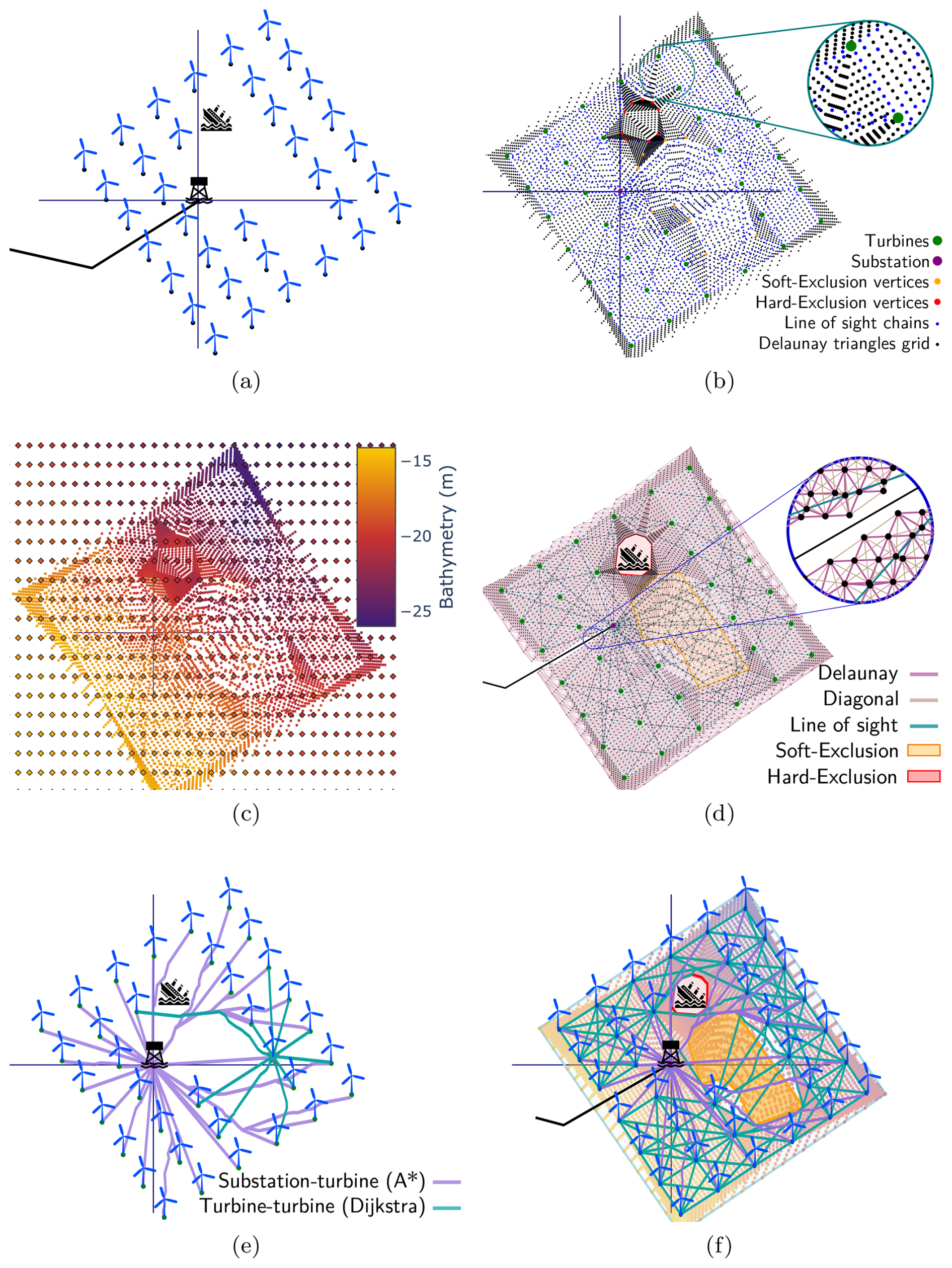
Figure 1Graph edge preparation procedure: (a) input layout, turbine group and substation; (b) grid densification, spatial grid for intermediate points; (c) terrain overlay, elevation or bathymetry data; (d) feasible graph, densified graph after spatial constraints; (e) shortest paths, feasible inter-turbine paths; (f) candidate graph, final graph used in the MILP optimisation.
The second stage of the array-optimisation process involves taking the undirected graph of feasible edges and selecting a configuration that minimises the total connection weight required to link all turbines to the substations. To achieve this, a MILP is formulated. The associated constraints are designed to enforce a radial array topology, limit the maximum number of turbines connected per string, and prevent edge crossings. As introduced above, a radial array is defined as a set of cable strings connecting turbines to substations without cycles. Each turbine lies on a simple path to a substation and may connect to at most two neighbouring nodes. The routing formulation uses the network sets, edge-flow variables, binary edge-activation variables, and routing parameters summarised in Appendix A and Sects. A1–A3.
3.1 Core formulation
The graph nodes (𝒩ac) are initially partitioned into two sets: turbine nodes 𝒩t⊆𝒩ac and substation nodes 𝒩s⊆𝒩ac, such that . To maintain power flow tracking within the system, each turbine node injects one unit of power, modelled as a fixed parameter such that pi=1 for all i∈𝒩t.
For substation nodes, the net injection is modelled as an integer decision variable representing power withdrawal, such that for all i∈𝒩s.
Power balance is enforced by requiring that the total substation withdrawal matches the total turbine injection:
Units of power are transferred through each edge and an integer variable fa∈ℤ is associated with each candidate edge a∈ℰ, representing the number of turbine units transmitted between nodes i and k. Although the graph is undirected, each edge is assigned an arbitrary reference orientation for flow accounting purposes. A negative value of fa therefore indicates flow opposite the chosen orientation. The following constraint ensures that the power generated by all turbines is transmitted through the grid and that no turbine remains unconnected:
To determine whether an edge is selected within the system, a binary variable is assigned to each candidate edge, indicating whether the corresponding edge is activated. To guide the optimisation towards selecting an appropriate number of edges, the following constraint is introduced:
This constraint states that the minimum number of edges required to interconnect all nodes in a single graph is one less than the number of nodes. Accordingly, the number of edges necessary to connect all turbines to a given number of disjoint substations can be determined, resulting in the formation of separate graphs within the wind farm structure.
Furthermore, the binary variable enables the restriction of crossing pair activations, ensuring that at most one edge from each crossing pair is active. Crossing pairs are defined by the set 𝒳 which denotes the set of unordered edge pairs (a,b) such that edges a and b geometrically intersect, as constrained by
To limit the maximum number of turbines connected via a single string, the power flow on each edge is constrained such that
Here, 𝔐 is a parameter that represents the maximum allowable integer power flow per edge, equivalent to the maximum number of turbines per string, and ξa ensures that no power is permitted through inactive edges. To regulate the number of permissible connections at each turbine node, the following constraint is imposed, limiting the number of active edges connected to each turbine node.
This is achieved by summing the binary activation values over the subset ℰi⊂ℰ of edges connected to node i. In radial arrays, this threshold is set to two for turbine nodes, ensuring that each turbine is connected to at most two active edges and thereby preventing bifurcations. Relaxing this constraint permits bifurcations and enables radial-star configurations when required.
A key consideration in the design of array systems is the number of permissible string connections to a substation. This is enforced by the following constraints:
Here, 𝔖s denotes the maximum number of string connections permitted at each substation node i∈𝒩s and is treated as a fixed integer within each MILP solve. To reduce the search space, the minimum number of string connections per substation, 𝔰s, determines the distribution according to the maximum number of turbines permitted in each string.
The objective of the optimisation is to minimise the total weight of all active edges, defined as
Here, 𝒲a denotes the pre-computed weight of edge a obtained during the graph preparation step (e).
3.2 Additional design constraints
To improve the practicality and balance of the solutions produced by the core MILP formulation, additional modelling strategies are introduced. These refinements aim to guide the optimisation process towards routings that are not only feasible but also well-structured in terms of string distribution and substation connectivity.
3.2.1 Minimum turbines per string
Another sub-strategy to balance strings involves enforcing a minimum number of turbines per string. To achieve this, we define the subset ℰs⊆ℰ, comprising edges that connect turbines to a substation, drawn from the set of all permissible graph edges. Certain considerations must be taken into account for any edge a∈ℰs. Firstly, for turbine–substation connections, the edge is treated as directed from the turbine to the substation, denoted as with i∈𝒩t and k∈𝒩s. This convention preserves the logic of Eq. (2), enabling the introduction of the following inequality constraint:
Here, 𝔪 denotes the minimum turbine unit flow per string. To balance the number of turbines per string based on 𝔐, the minimum number of connections to the substations is determined from Eq. (7). Following this logic, 𝔪 can be calculated as
For example, in an array group comprising 50 turbines, and assuming a maximum string capacity of seven, the minimum number of connections to the substation is eight, whereas the minimum number of turbines per string is six.
3.2.2 Determination of substation connections
Due to connectivity and crossing constraints, determining an appropriate value for the number of substation connections is not always straightforward. If the range between 𝔰s and 𝔖s is too large, the algorithm may produce numerous very short strings, resulting in an unbalanced electrical grid. To mitigate this, a simple iterative algorithm is employed. It determines the minimum feasible value of the maximum number of substation connections, 𝔖s, required to ensure full turbine connectivity.
The algorithm begins by computing the ceiling of the division of the number of turbines by the product of the number of substations and the maximum number of turbines per string, as shown in Eq. (7b), and setting 𝔖s=𝔰s. This estimate aims to distribute the strings evenly across substations. If the resulting routing is infeasible, the value of 𝔖s is incrementally increased by one until a feasible solution is found.
As the required connections to the substation increase at each iteration, if the determination of the number of substation connections is combined with the minimum number of turbines per string, Eq. (10) must be modified to use the maximum bound, such that
3.2.3 Unbalanced substation capacity
In certain projects, circumstances may necessitate the installation of substations with differing capacities, such as in spatially separated development areas. In such cases, constraint Eq. (1) must be further specified as follows:
Here, each substation is limited by a maximum per-unit capacity, denoted by . The inequality is formulated such that the flow is greater than or equal to the limit because pi represents the outgoing flow of the system and is assumed to take negative values. To accommodate differing capacities, it is required that the total installed capacity across all substations equals or exceeds the number of turbines, as specified in Eq. (12b), which acts as a consistency condition on the user-defined input parameters rather than a constraint involving optimisation variables, since substation capacities are fixed inputs and not subject to optimisation.
The conductor size selection (CSS) problem determines the appropriate diameter for each cable section from a restricted set of available park conductor types. For every connection between two nodes, a cable type ι must be selected from the mutually exclusive set ℐ, allowing only one conductor type per connection.
In this section, the CSS problem is formulated assuming that the network routing has already been determined. Let 𝒜⊆ℰ denote the subset of active edges selected during the routing stage, such that ξa=1 for all a∈𝒜. Under this formulation, the optimisation assigns a conductor type to each active connection such that the power flow requirements are satisfied while minimising the total conductor investment cost. Each conductor type ι∈ℐ is characterised by a conductor cost per unit of length ψι. Accordingly, the objective function is defined as
Here, ξa,ι is a binary variable indicating whether conductor type ι is assigned to edge a, and La denotes the pre-computed length of edge a obtained during the graph preparation step (e). The CSS formulations use the active-edge set, conductor-type set, conductor-selection variables, electrical quantities, and economic parameters summarised in Appendix A, Sects. A1, A2, A4, and A5.
4.1 Non-linear CSS
One possible formulation for cable size selection employs a non-linear model of AC power flow (ACOPF). This formulation considers the voltage magnitude V and angle θ at each node and calculates the active P and reactive Q power flowing in each branch based on the branch admittance representation derived from . The apparent power Sik from node i to node k is then defined as
Each node i∈𝒩ac is assumed to correspond to either a turbine or a substation, such that at most one of or is non-zero. Accordingly, the nodal power balance is given by
Here, variables and denote the active and reactive power generated at node i by a connected turbine, while and represent the corresponding substation consumption. The term represents curtailed generation, where .
This allows consideration of the trade-off between system losses and cable investment costs. Non-linear modelling captures the complete π model of cables, including inductance and, crucially for submarine cables, capacitance, which can increase reactive power and thereby lead to additional losses. The formulation of a non-linear CSS power flow is presented in Valerio et al. (2026a), where each array section a includes multiple Ybus-branch elements corresponding to the various conductor types that may connect the node pair, as illustrated in Fig. 2.
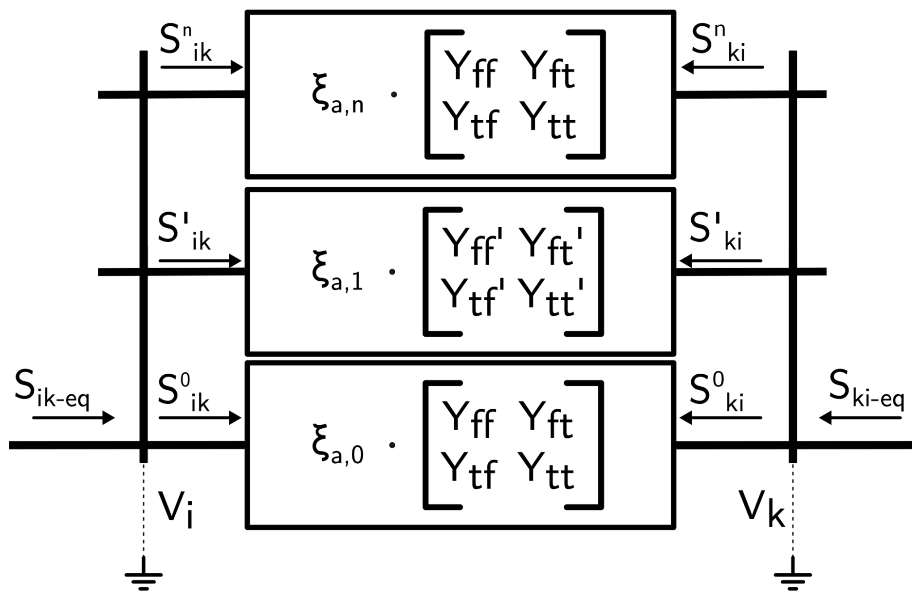
The use of equivalent bus admittance matrices establishes a relationship in which the power at each end of the equivalent branch is determined by multiple binary factors , which relate the apparent power flow associated with each conductor type, Sa,ι, to the equivalent branch flows and , such that
Here, denotes the apparent power flow associated with conductor type ι on branch , directed from node i to node k, where ξa,ι is indexed by both the branch position a and the conductor type ι∈ℐ. The referenced paper presents a non-linear approach that considers internal system losses, allowing for the intentional over-sizing of conductor sections to reduce losses. These losses are incorporated into the main CSS objective within a multi-objective framework as follows:
Here, the losses are calculated as the total available power to be injected by the turbines, , minus the total power extracted by the substations, , in the array system. The economic parameter Hy denotes the full-load hours of system operation over y years, while ρ denotes the electricity cost, for example based on an assumed LCoE. The discount rate r enables a net present value (NPV) comparison with conductor investment costs. Both individual objectives are combined into a multi-objective function using a weighting parameter , which determines the relative importance of the loss-related term,
4.2 Linear CSS
While non-linear modelling provides the most comprehensive representation of losses and power flow, it can be computationally intensive. If efficiency is a priority, a strategy based on a linear simplification of power flows, commonly referred to as the DCOPF approximation, can be adopted. This subsection presents the corresponding equality and inequality constraints associated with this formulation.
4.2.1 Equality constraints
The linear power flow approximation assumes that voltage magnitudes remain constant and close to one per unit at all nodes, while the voltage angle differences between connected nodes are small. Under these assumptions, the AC power flow equation simplifies to
Here, the active power flow is computed using the negative imaginary part of the corresponding Ybus entry for each conductor.
To establish the real power balance at each node, the equivalent formulation equates the net power injection from turbines (t) and substations (s) to the corresponding power flows within the system:
Following Eq. (16), the equivalent real power flow across each connection is described by Eq. (21a). However, to avoid introducing a quadratic constraint resulting from the product of binary and continuous variables, McCormick envelopes are applied using auxiliary variables za,ι:
To support this linearisation, a big-M parameter is introduced to relax specific constraints involving binary variables. In this study, it is defined in Eq. (22), where Ma represents the maximum allowable power for any conductor type in branch a, scaled by a security factor κ. The value of κ is set to 1.1. This parameter acts as an upper bound, effectively deactivating flow constraints when the corresponding binary variable indicates that the conductor is not selected:
Importantly, Ma is defined separately for each branch to keep the big-M value as tight as possible based on the available conductor capacities. A single global big-M value could also be used, but this may introduce unnecessarily large bounds for some branches, resulting in a weaker relaxation and reduced computational performance.
4.2.2 Inequality constraints
The McCormick envelopes are constructed such that Eq. (23a) and (23b) enforce an equality between z and P when ξ is active. When ξ is inactive, both constraints are relaxed by the maximum power Ma, ensuring feasibility regardless of flow. In addition, Eq. (23c) and (23d) define the bounds on z: when ξ is active, these bounds correspond to the maximum power permitted by the selected conductor; when inactive, z is constrained to zero.
Thermal limits for each branch are enforced by bounding the flow to comply with criterion C3. The following constraints implement this limitation, with activation governed by ξa,ι. When inactive, the constraints are relaxed using the big-M formulation:
For the CSS selection, one conductor must be chosen for each section, as enforced by the following constraint:
To track which conductor types are used in the overall system and comply with criteria C5, the binary indicator is introduced. This indicator identifies whether conductor type ι is active within the system. The following constraints ensure that νι is assigned consistently. In particular, Eq. (26a) enforces that if one or more ξa,ι values are active across any connection a, then νι must be set to one, whereas Eq. (26b) ensures that if no ξa,ι variables are active for a given ι, then νι must be zero.
Here, 𝔑 denotes the user-defined maximum number of conductor types permitted in the system. As the decoupled CSS setting does not rely on the assumption that the array system forms a tree, the exact number of active edges in the system is unknown, particularly in the case of looped arrays. For this reason, constraint (Eq. 26) allows greater flexibility in the selection of conductor types.
In Sect. 4, conductor size selection was formulated assuming that the routing of the array system was already determined. Under this formulation, cable diameters are assigned to a fixed network topology. However, the routing configuration and conductor sizing are inherently coupled, since limiting the set of conductor types also limits the maximum transferable power within the network. Importantly, this limit is determined not by the largest conductor type available overall but by the largest conductor type selected for use in the network.
To account for this interaction, conductor size selection can be coupled with the routing formulation. This allows routing decisions and conductor assignments to be evaluated within a coordinated optimisation framework. Two strategies are considered: an integrated formulation (Sect. 5.1) and a sequential algorithm (Sect. 5.2).
5.1 Integrated conductor size selection
In the integrated formulation, conductor size selection is incorporated directly into the routing optimisation. Each candidate edge may therefore be associated with multiple conductor types, and the optimisation determines both whether the edge is activated and which conductor type is assigned.
Each conductor type ι∈ℐ is characterised by a flow capacity 𝔐ι. To represent the assignment of conductor types to candidate edges, the binary edge-activation variable is extended with an additional dimension ξa,ι associated with each branch. This variable links the activation of an edge to the selection of a specific cable type, such that
Here, the sum of assigned conductor types equals one if the branch is active and zero otherwise. As the flow limit now depends on the selected conductor type, Eq. (5) is modified to reflect type-specific capacities:
In this formulation, the parameter 𝔐 used in Eq. (7) is defined as the maximum value over all conductor capacities, i.e. , ensuring that each branch satisfies criterion C3. To constrain the permissible number of active conductor types from the set and comply with criterion C5, the previously defined binary variable νι is employed. Leveraging Eq. (3), which defines the total number of active branches based on the number of turbines and substations, the term provides an upper bound on the number of branches. Accordingly, Eq. (26a) is reformulated as follows:
The objective of the optimisation is to minimise the total cost of all active edges as follows:
Here, ψι and ψa represent the cost per unit of length of each cable type and the installation cost per unit of length respectively. It is important to note that installation costs are based on the weighted length 𝒲a, which accounts for soft exclusions from graph preparation (d, e), while conductor costs are based on the actual length La of each segment. The objective thus captures a combined cost of installation and cable type selection.
However, the inclusion of cable size selection is mutually exclusive with the iterative determination of substation connections, as the computation of the initial connection set-point to the substation depends on the largest conductor used. If this is decided in advance, it constrains the space of possible solutions.
5.2 Sequential algorithm
To address this limitation, a sequential approach is proposed. This formulation allows the routing stage to incorporate more detailed constraints that would otherwise overly restrict the integrated optimisation problem. However, it also highlights a limitation of single-pass routing approaches. When routing is performed independently of CSS, the routing stage primarily minimises geometric length, while conductor costs are determined only subsequently during cable size selection. As illustrated in Fig. 3a, the relationship between conductor cross-sectional area and power capacity is sublinear, such that progressively larger increases in conductor cross-sectional area are required to accommodate additional power. Furthermore, Fig. 3b shows that higher-capacity conductors incur disproportionately greater costs. Therefore, the shortest trench or cable routing typically concentrates power into fewer, larger conductors and does not necessarily correspond to the minimum total investment cost, as the routing stage optimises geometric cable length independently of conductor costs.
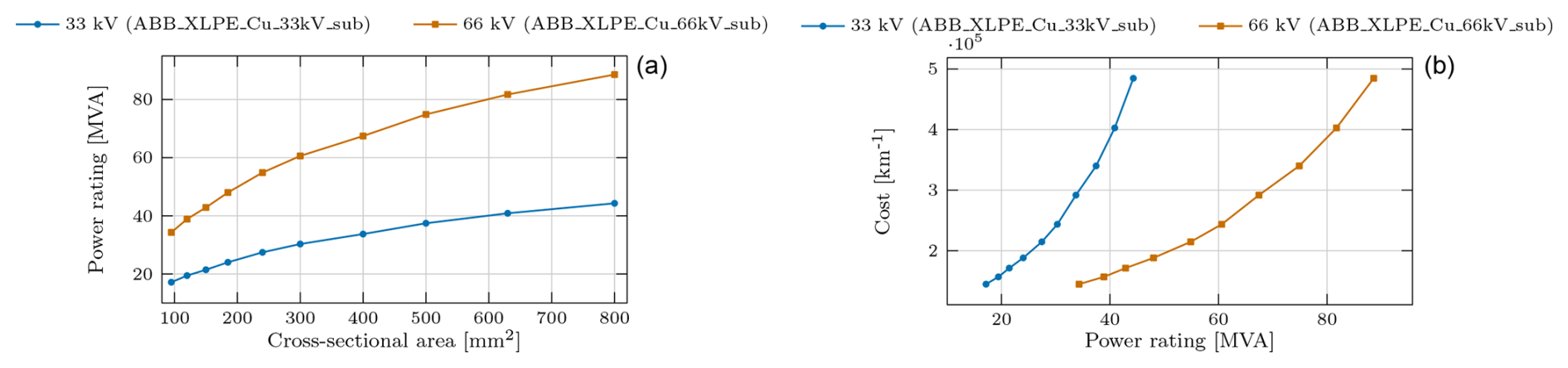
Figure 3Relationship between conductor cross-sectional area, power capacity, and cost: (a) cross-sectional area versus power rating; (b) power rating versus cost.
This mismatch is further influenced by the definition of the maximum number of turbines per string, 𝔐, which is based on the capacity of the largest available conductor. Consequently, routing solutions that minimise cable length tend to favour configurations with a larger number of turbines per feeder, implicitly encouraging the use of higher-capacity cables and potentially increasing the overall investment cost.
The sequential algorithm, illustrated in Fig. 4, addresses this issue by iterating between routing and conductor sizing decisions. The procedure begins with the graph prepared using the method described in Sect. 2 and considers a set of possible conductor types ℐ. In the first iteration, the minimum path connection problem (Sect. 3) is solved in conjunction with the substation connection strategy described in Sect. 3.2.2 to determine the trenching investment cost, denoted by ΨMP. The resulting subset of edges determined by the routing optimisation, 𝒜, is then evaluated using either a non-linear CSS approach (Sect. 4.1), which accounts for conductor losses and investment, or a linear CSS model (Sect. 4.2), which focuses solely on conductor investment and is computationally more efficient.
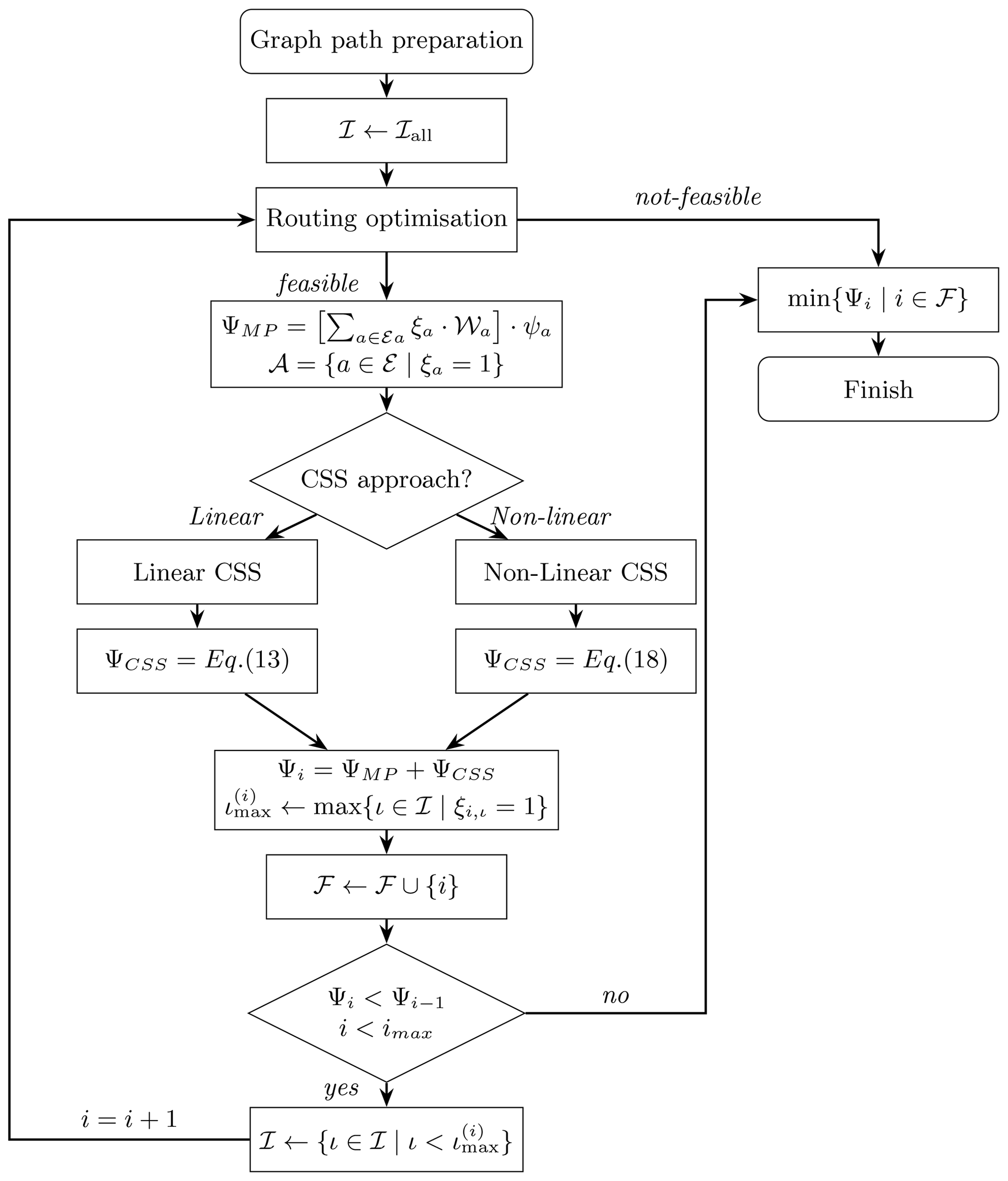
Figure 4Sequential routing–CSS algorithm: routing, determine the active edge set for the current conductor set; CSS, size the selected connections using the linear or non-linear formulation; evaluation, compute the total routing and conductor investment cost; update, restrict the conductor set and repeat until no further cost reduction is obtained.
Following the CSS assignment, the total cost Ψi for iteration i is calculated by summing the trenching and conductor investment costs. The largest conductor type used in that iteration, denoted , is then identified. The solution is subsequently added to the feasible solution set ℱ.
In the subsequent iteration, the candidate conductor set ℐ is restricted to conductor types with capacities strictly smaller than , and the procedure is repeated. This progressively limits the search to solutions relying on smaller conductor types. The algorithm terminates under three conditions: (i) if the routing problem becomes infeasible, for example due to path limitations, a restricted number of allowable substation connections, or an empty conductor set or (ii) if the user-defined iteration limit is reached, or (iii) if the reduction in conductor costs achieved by using smaller cable types is outweighed by the increase in trenching costs due to longer routing distances, resulting in a higher total cost than in the previous iteration.
The final array configuration is selected as the solution with the minimum total cost from the feasible solution set ℱ.
In this section, case studies are presented to illustrate the methodology. First, a set of case studies focuses solely on the routing MILP model and demonstrates how its adaptations result in different solutions. Second, offshore and onshore case studies are used to compare the multi-stage methodology when adopting either an integrated or a sequential approach. Finally, two wind parks are utilised to compare the use of linear and non-linear CSS within the sequential framework. The case studies presented in this paper are based on existing offshore and onshore wind parks in order to demonstrate the scope of the formulation. However, they cannot be directly compared with real projects, as the authors do not have access to internal cost data or to the specific technical details of the cables used in these developments. The data associated with the case studies, including array voltage, turbine rated power, and graph creation results from Sect. 2, such as the number of nodes, edges, crossings, and graph generation time, are presented in Appendix B, while the conductor type data are presented in Appendix C.
6.1 Collector-system routing modelling
To provide a visual example of the routing formulation and its refinements, the turbine distributions of Baltic Eagle [DE] and Moray East [GB-SCT] are used. Based on the turbine and substation locations, several tests are conducted. The evaluated formulations, summarised in Table 1, are identified using the following short descriptive handles.
-
Core: core formulation for determining minimum paths (Sect. 3.1)
-
Minimum turbines: inclusion of a constraint on the minimum number of turbines per string (Sect. 3.2.1)
-
Substation connections: refinement of the formulation to determine substation connections (Sect. 3.2.2)
-
Joint constraints: simultaneous inclusion of the minimum-turbine and substation-connection restrictions
-
Bifurcation: relaxation of constraint (Eq. 6) to allow bifurcations
-
Additional substation: for Baltic Eagle [DE], inclusion of a hypothetical additional substation limited to a maximum of 10 turbines, illustrating substations with different power limits (Sect. 3.2.3)
The corresponding cable routing solutions are shown in Fig. 5 for Baltic Eagle [DE] and Fig. 6 for Moray East [GB-SCT].

Figure 5Baltic Eagle [DE] array results: solutions from model parameters set to (a) core formulation, (b) minimum number of turbines per string, (c) allowing bifurcations, and (d) irregular substation capacities.
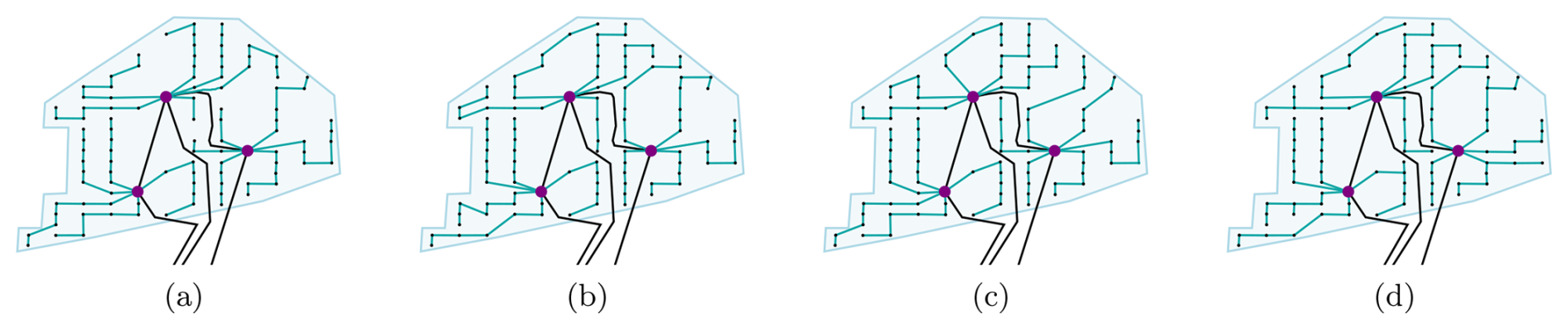
Figure 6Moray East [GB-SCT] array results: solutions from model parameters set to (a) core formulation, (b) determining substation connections, (c) minimum number of turbines per string and determining substation connection, and (d) allowing bifurcations.
Table 1Baltic Eagle [DE] and Moray East [GB-SCT] minimum path-finding solutions.
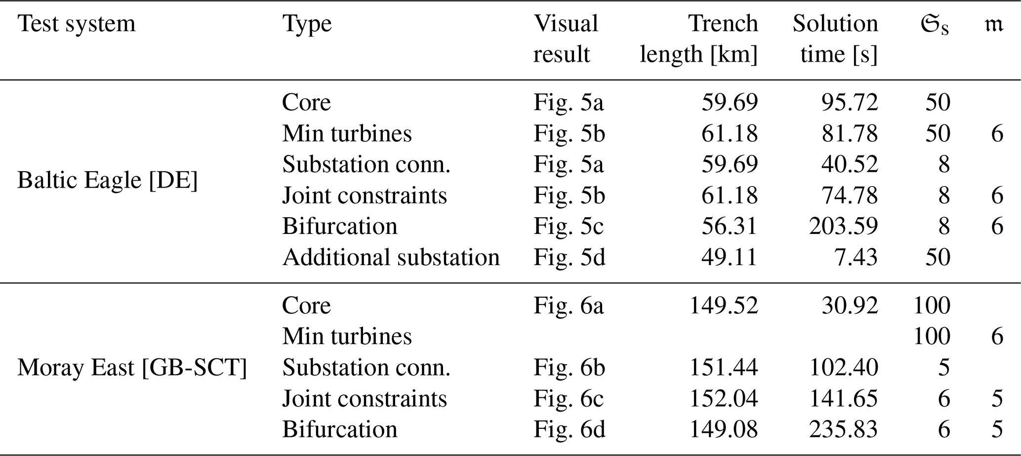
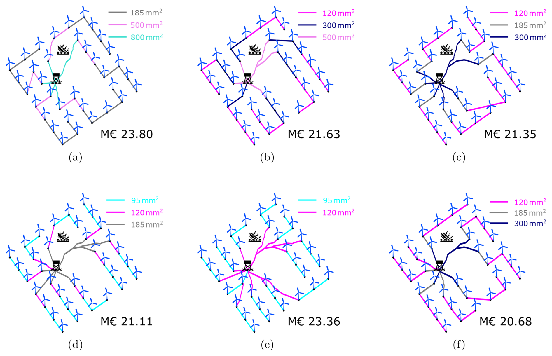
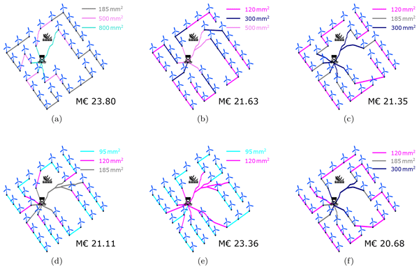
Figure 7Westermost Rough [GB-ENG] array results: iterative solutions from (a) iteration 1 to (e) iteration 5, and (f) the integrated MILP formulation.
As shown in Fig. 5, the core formulation yields short strings that are balanced according to the minimum turbines-per-string constraint. However, for the Moray East [GB-SCT] case, the algorithm fails to produce a feasible solution under the minimum turbines-per-string criterion within the specified parameters, owing to limitations on inter-substation connectivity. In the subsequent formulation, where the minimum number of substation connections is determined iteratively, the solution time is reduced in both cases.
As illustrated in Table 1, relaxing the constraint (Eq. 6) to allow radial-star configurations results in shorter trench lengths in both cases, although at higher computational cost. Since radial configurations are a subset of radial-star configurations, the resulting system routings cannot be shorter than those obtained with bifurcations; however, the reduced solution space can aid the solver in approaching optimality.
6.2 Test systems for joint optimisation
To enable broad application of the formulation, a cable database was created. For offshore cases, the database is based on copper cables from ABB (2010b) and includes 22, 33, and 66 kV voltage levels, covering 10 conductor cross-sectional areas ranging from 95 to 1000 mm2. For onshore cases, the database is based on copper cables from ABB (2010a) at the 33 kV voltage level, covering 15 cross-sectional areas from 95 to 2000 mm2, assuming buried cables under trefoil conditions.
In all simulations, the cost per metre of each conductor type is estimated using the procedure described in Dicorato et al. (2011), which relates cost to the conductors cross-sectional area. Based on the same reference, a trenching cost of 304 k EUR km−1 is used in offshore simulations. For onshore simulations, the trenching cost is assumed to be half this value, as no reliable public data were found.
In each case study, the number of conductor types is limited to 𝔑=3, meaning that at most three conductor types from the cable database may be selected in the optimisation. In addition, no explicit general constraint is imposed on substation connections. Both the cable database and the implementation of the methodology are available in the repository (Valerio et al., 2025). Simulations were performed on a desktop computer equipped with a 12th Gen Intel® Core™, i5-12400 processor (2.50 GHz) and 64 GB of RAM. The Gurobi solver (Gurobi Optimization, LLC, 2026) was used to solve the mixed-integer linear problems.
For the integrated approach, a time limit of 6 h (21 600 s) was imposed. In contrast, the sequential approach used a time limit of 1.5 h (5400 s) per sub-problem; therefore, the total runtime may exceed this limit depending on the number of iterations required. In the sequential approach, all CSS evaluations are performed using the linear formulation presented in Sect. 4.
To illustrate the joint routing and conductor optimisation, the case of Westermost Rough [GB-ENG] is first presented. This example uses the same graph shown in Fig. 1f. For the sequential approach, the intermediate results of the algorithm iterations are depicted in Fig. 7a–e.
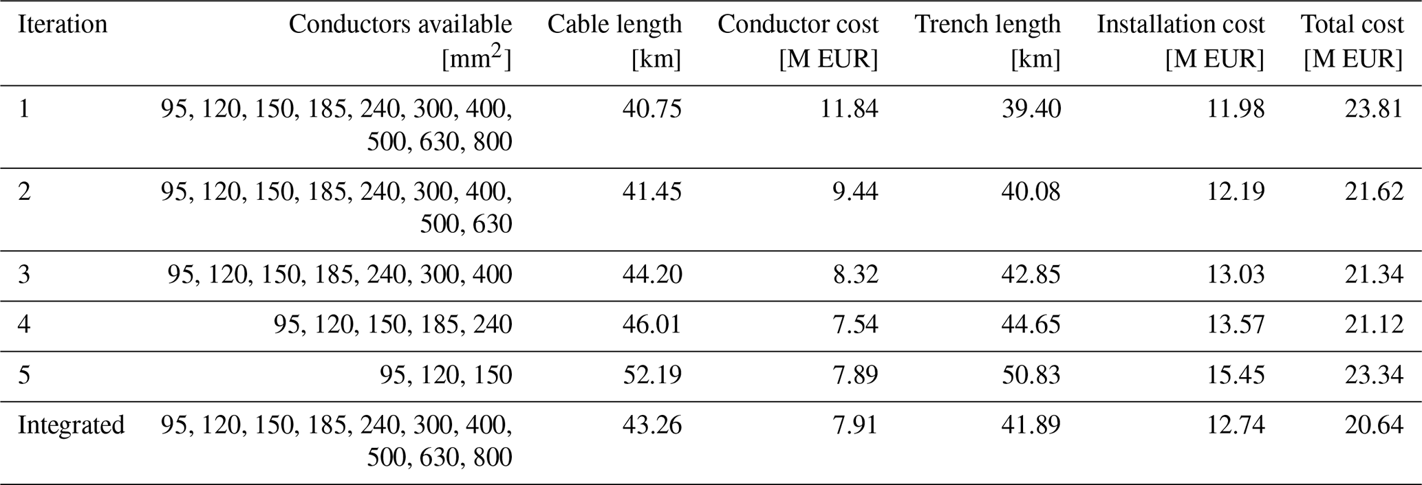
In the first iteration, with all 10 conductor capacities available, the minimum-route solution connects seven turbines per string, requiring a conductor size of 800 mm2. In the second iteration, the 800 and 1000 mm2 conductors are excluded from the available options. The process continues until iteration five, where the total investment exceeds that of iteration four. The resulting optimal configuration includes cable types of 95, 120, and 185 mm2.
For comparison, the integrated CSS result is shown in Fig. 7f. This result uses the same conductor selection as iteration three of the sequential algorithm (see Fig. 7c). In iteration three, the connections to the substation are determined within the optimisation. In contrast, the integrated CSS does not perform this evaluation, allowing the algorithm to generate shorter strings, assign the 300 mm2 conductor to only three strings, and increase the total number of strings, thereby reducing the overall cost. A detailed cost breakdown is provided in Table 2, where increases in cable length, trench length, and installation cost can be observed as the iterations progress; however, the total cost continues to decrease until the reduction in conductor costs no longer compensates for the additional trenching.
Table 2Westermost Rough [GB-ENG] sequential compared to result of integrated approach array costs.
Note: M EUR: million euros.
Further case studies were implemented, covering wind parks ranging from 12 to 174 turbines, with power capacities between 2 and 14 MW, and including arrays with one to three substations. Detailed information on the number of permissible edges, number of turbines, identified crossings, and turbine power and voltage is given in Table B1. The table also reports the graph preparation time for each case.
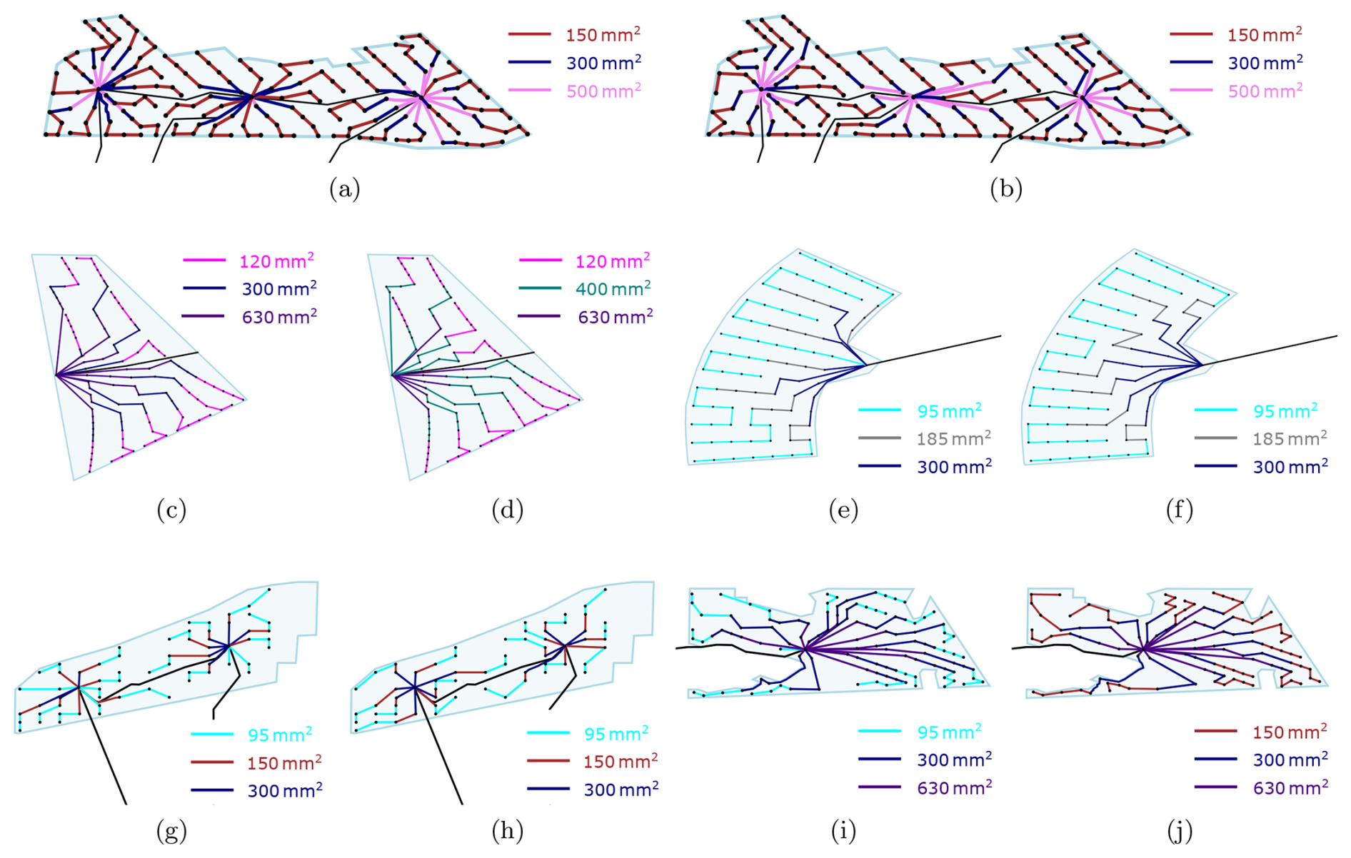
Figure 8Offshore array results showing integrated and sequential CSS solutions respectively for each case: (a, b) Hornsea I [GB-ENG], (c, d) Anholt [DK], (e, f) Horns Rev 2 [DK], (g, h) Moray West [GB-SCT], and (i, j) Seagreen [GB-SCT].
Hornsea I [GB-ENG] (Fig. 8a, b) serves as the largest test case, with 174 turbines and three substations. Anholt [DK] (Fig. 8c, d) highlights how inter-turbine edges are prevented from crossing export cables, in this case due to the connection from Anholt Island to Denmark. Horn Rev 2 [DK] (Fig. 8e, f) illustrates the effect of the sequential balancing constraints, which favour a more even distribution of turbines across strings than in the integrated solution. Moray West [GB-SCT] (Fig. 8g, h) exemplifies configurations with large-capacity turbines. Seagreen [GB-SCT] (Fig. 8i, j) demonstrates the use of irregular development areas, where densification of points generates non-standard edges that comply with spatial constraints.
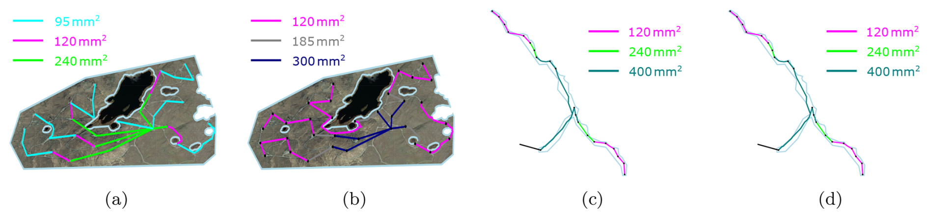
Figure 9Onshore array results showing integrated and sequential CSS solutions respectively for each case: (a, b) Bhlaraidh [GB-SCT] and (c, d) Coromuel [MX].
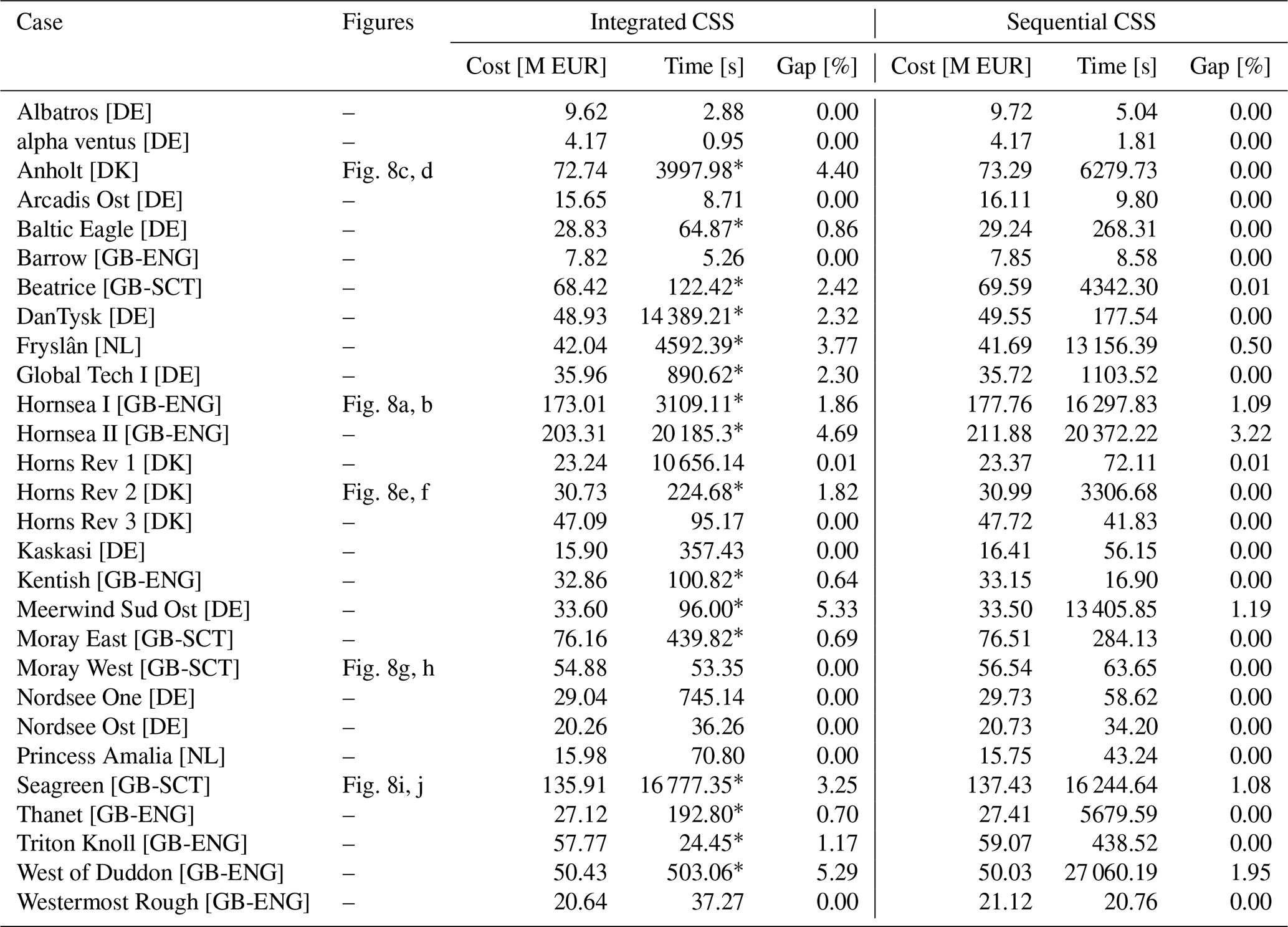
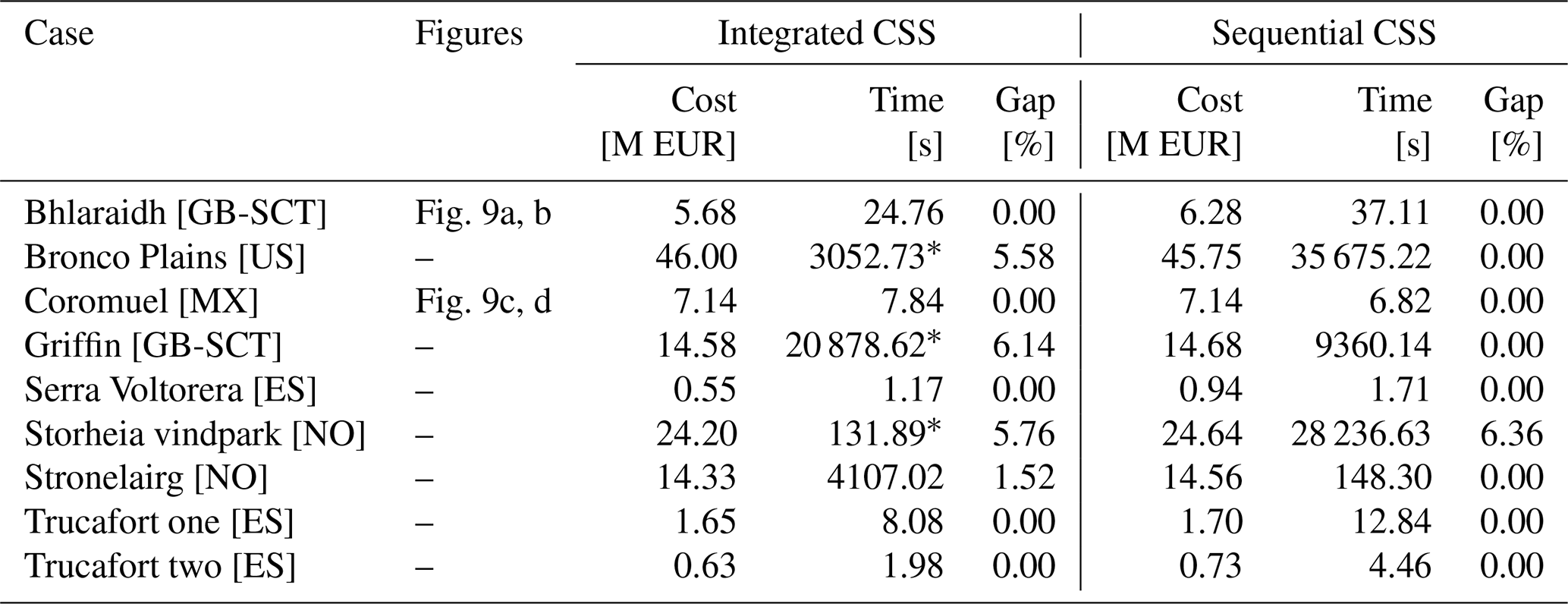
Table 3 summarises all offshore test cases, reporting the objective value, solution time, and the final optimality gap if the time limit was reached. The optimality gap measures the difference between the best feasible solution and the solver's lower bound, which comes from LP relaxations and represents a provable bound on the optimal objective (Gurobi Optimization, LLC, 2026). Simulation times marked with an asterisk (*) indicate when the last feasible solution was obtained. Detailed results are given in Tables D1 and D2 of the individual objective costs.
In the onshore cases, the z plane incorporates elevation, with inclination playing a more significant role in further limiting the connectivity of the densified points. The test cases cover wind parks ranging from 10 to 106 turbines, with power capacities between 225 kW and 3.6 MW. Detailed information on the number of permissible edges, number of turbines, identified crossings, and turbine power and voltage is given in Table B1.
For example, Bhlaraidh [GB-SCT] (Fig. 9a, b) illustrates the role of exclusion zones in routing around waterbodies such as lakes, while Coromuel [MX] (Fig. 9c, d) demonstrates that the algorithm can still achieve feasible solutions in highly constrained development areas. Finally, Table 4 summarises all onshore test cases, reporting the objective value, solution time, and the final optimality gap if the time limit is reached. Simulation times marked with an asterisk (*) indicate when the last feasible solution was obtained. The results are given in more detail in Tables D1 and D2 of the individual objective costs.
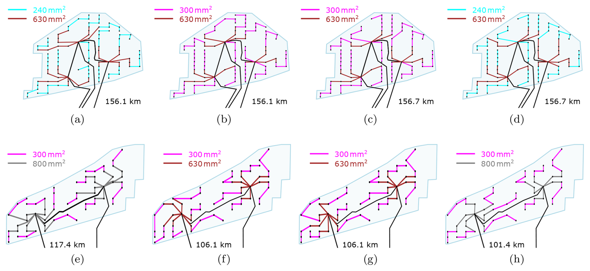
Figure 10Project comparison for Moray East (a–d) and Moray West (e–h) [GB-SCT]: actual reported collector-system routings and routings obtained using the integrated, linear sequential, and non-linear sequential methodologies.
6.3 Comparison with non-linear CSS approach
To bridge the difference to comparable project data, the inter-array documentation for Moray East [GB-SCT] (Marine Scotland, 2019) and Moray West [GB-SCT] (Marine Scotland, 2022) are used as a reference. In the simulations, cable selection is restricted to two aluminium types, with a maximum of eight and six strings per substation for Moray East [GB-SCT] and Moray West [GB-SCT] respectively.
The simulation utilises four aluminium conductors, defined based on the cable capacities reported in Marine Scotland (2019, 2022) for conductor sizes of 240, 300, 650, and 800 mm2, as well as technical data and cost approximations from ABB (2010b) and Dicorato et al. (2011). The project documentation specifies the cable length used for each conductor size, and for comparability, costs are calculated based on the same costs per length as those used in the simulations. The reported routing for Moray East [GB-SCT] is reproduced in Fig. 10a for comparison with Fig. 10b, c, and d, while the reported routing for Moray West [GB-SCT] is presented in Fig. 10e and compared with Fig. 10f, g, and h, which show the resulting routings from the integrated and sequential methodologies, which respectively show the simulation of the integrated, linear sequential, and non-linear sequential approaches.
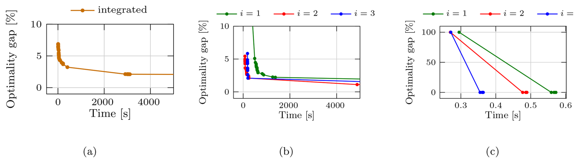
Figure 11Solver progress for the case Hornsea I [GB-ENG]: (a) integrated CSS-MILP, (b) sequential: minimum path connection with minimum turbines and determining substation connections, and (c) sequential: CSS.
To account for losses, a non-linear approach is applied. Assuming an LCoE of EUR 91 per MWh and 5170 full-load hours annually over a 25-year project lifetime (Kost et al., 2024), a net present value analysis of losses relative to investment is conducted. Electrical losses are obtained from the ACOPF solution at the equivalent full-load operating point and are converted to lifetime cost using the assumed full-load hours. To enable a direct comparison between losses and investment costs, the value of α in Eq. (18) is set to 1. For the non-linear simulation, the sequential algorithm is executed in a WSL environment, using OR-Tools (Perron and Furnon, 2025) for routing and Bonmin (Bonami et al., 2008) for the CSS.
In both cases, the non-linear CSS shown in Fig. 10d and h differs in conductor size selection from the linear solutions, while more closely resembling the reported project data. Comparing the linear and non-linear CSS for Moray East, the use of smaller conductor capacities is reduced, whereas higher-capacity conductors are utilised across a greater number of connections. In the case of Moray West, two strings connect six turbines instead of five, requiring a higher-capacity cable.
For a comparable assessment, losses are also calculated using a Newton–Raphson power flow applied to the grids obtained from the linear approaches. These results are presented in Table 5.
Marine Scotland (2019)Marine Scotland (2022)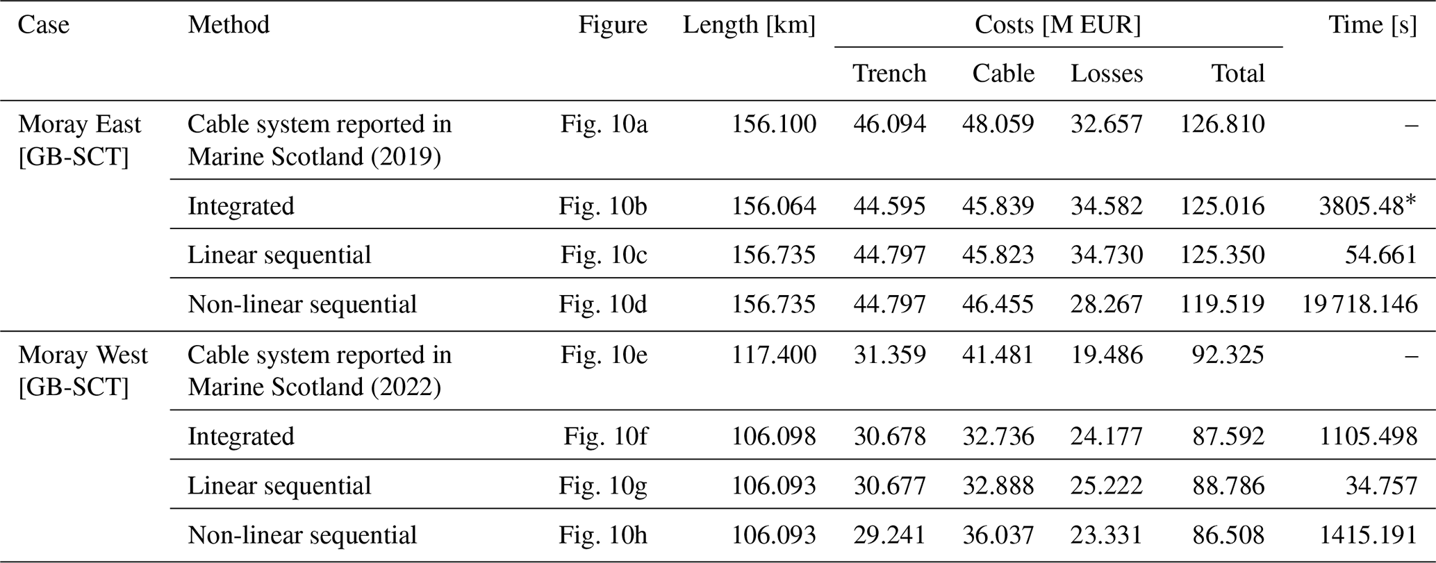
The test systems presented above demonstrate the application of the graph preparation methodology, followed either by an integrated formulation of a mixed-integer linear programming model to address the routing task and conductor size selection or by a sequential methodology that treats both problems separately. The iterative algorithm is designed to balance the allocation of turbines within strings and the distribution of strings across multiple substations. Where feasible, the algorithm favours equal string sizes. When this is not possible due to buildable-area constraints, the optimisation starts from the closest feasible configuration.
The routing algorithm presents a core formulation that can be adapted to user requirements, as illustrated in Sect. 3.2, with potential for broader application. In the examples provided, the turbine layouts of Baltic Eagle [DE] and Moray East [GB-SCT] are used to illustrate comparisons across various optimisation objectives, including minimising the number of turbines per string, reducing the number of strings per substation, comparing configurations with radial-star routing, and incorporating substations with limited power capacities.
Shifting focus to full-park optimisation with CSS, as presented in Sect. 6.2, the integrated results reveal that in most cases the optimisation reaches the imposed time limit. However, feasible solutions are typically identified within a relatively short time window, after which the optimisation primarily focuses on reducing the optimality gap. Although the gap generally decreases over time, convergence can be slow, making it difficult to prove optimality within practical computational limits. Consequently, selecting an appropriate cut-off time that balances computational effort and solution quality remains non-trivial. For example, in the case of Griffin [GB-SCT], the last feasible solution is found very close to the time limit.
By contrast, when using the sequential solution, even simple turbine layouts tend to result in longer computation times, as the routing algorithm is executed repeatedly. In more complex turbine arrangements and constrained areas, the time limit is still often reached; however, because the underlying optimisation problem is simpler, the optimality gap is generally closed more efficiently. In Tables 3 and 4, the gap presented in the sequential CSS column refers to the optimality gap of the resulting iteration of the routing algorithm, which in all cases is smaller than that of the integrated approach or is zero.
The case studies presented above illustrate the application of the strategies to both offshore and onshore systems. In these cases, the algorithm determines the optimal combination of conductor sizes and pathways to interconnect all turbines. The algorithm achieved this under 5 s for the smaller systems. However, for the larger and more complex cases, the routing algorithm reached the predefined time limit. In such instances, while the solution is feasible, optimality cannot be guaranteed.
The problem is solved using the Gurobi solver, which applies a branch-and-bound algorithm to identify feasible solutions. Through the use of callbacks, the solver records both the objective value and the time at which each feasible solution is found. Solver progress for the Hornsea I test cases is illustrated in Fig. 11a for the integrated formulation, and in Fig. 11b and c for the sequential iterations of the routing and CSS stages respectively.
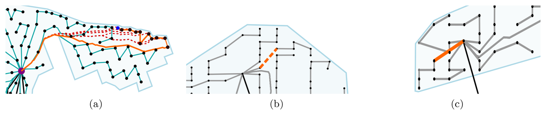
Figure 12Onshore array results showing integrated and sequential CSS solutions respectively for each case: (a) section of Hornsea II connectivity, (b) Moray East Delaunay and diagonals restriction, and (c) Moray West Static Crossings
Both Fig. 11a and b show rapid initial convergence, as reflected by the reduction in the optimality gap. The plots report the optimality gap at the moment each feasible solution is found. As the solver progresses, the lower bound may improve, meaning that the gap associated with earlier solutions would decrease if evaluated against the final bound. In Fig. 11c, the solver reaches optimality quickly, indicating that the CSS stage is not restrictive in terms of solution time. Consequently, the routing stage becomes the primary determinant of overall optimality, and simplifying this stage through sequential iterations proves beneficial.
An important extension of the sequential algorithm is the ability to employ a non-linear CSS formulation that accounts for electrical losses in the overall cost. In this paper, losses are evaluated using an equivalent full-load-hours analysis, in which each turbine operates at its rated power and the resulting network currents are obtained from the corresponding ACOPF. The non-linear formulation allows conductor cross-sectional areas to be increased to reduce resistive losses. However, excessive conductor sizing also increases cable capacitance and the associated charging losses. This trade-off is explicitly considered within the non-linear CSS optimisation.
7.1 Collector-system routing benchmarking
Several state-of-the-art cable-routing formulations represent each candidate connection through two directed arcs, allowing the optimiser to select the direction associated with power flow towards the substation (Fischetti and Pisinger, 2018a, b; Pérez-Rúa et al., 2020a). This provides a useful structural reference for the routing component of the proposed formulation. For the quantitative benchmark, however, OptiWindNet (Souza de Alencar et al., 2025) is selected because it is available as an open-source framework and directly addresses the spatial embedding of selected connections. Its search space is built from a sparsified candidate graph based on constrained Delaunay triangulation, diagonals, and feeder links. In particular, it goes beyond purely static crossing constraints by separating topology selection from route embedding, enabling non-straight cable routes and reducing the number of crossing constraints considered during optimisation. Gurobi was selected as the common solver for both approaches with a 6 h time limit. For cases reaching the imposed time limit, the reported value corresponds to the best incumbent solution.
The comparison is restricted to the routing component and uses total cable length and solution time as common metrics. Three test types were used to enable comparison across the case studies. The first was a non-restrictive test, in which no substation-connection limit was enforced and the maximum string length was set equal to the number of turbines in the wind park, . In the second test, the maximum number of turbines per string was set according to the highest-capacity conductor available for the corresponding voltage level, as reported in Sect. B. In the third test, substation connections were limited to obtain a more balanced string configuration. The resulting 𝔖s and 𝔐 values are shown in Table 7.
The first aspect evaluated is the problem size. Table 6 presents the number of variables and constraints considered by the solver. In the proposed formulation, the number of variables is reduced primarily because each candidate edge is represented by a single activation variable. However, the number of constraints increases substantially owing to the use of static crossing constraints.
Table 6Model size comparison between pyflow-acdc and OptiWindNet.
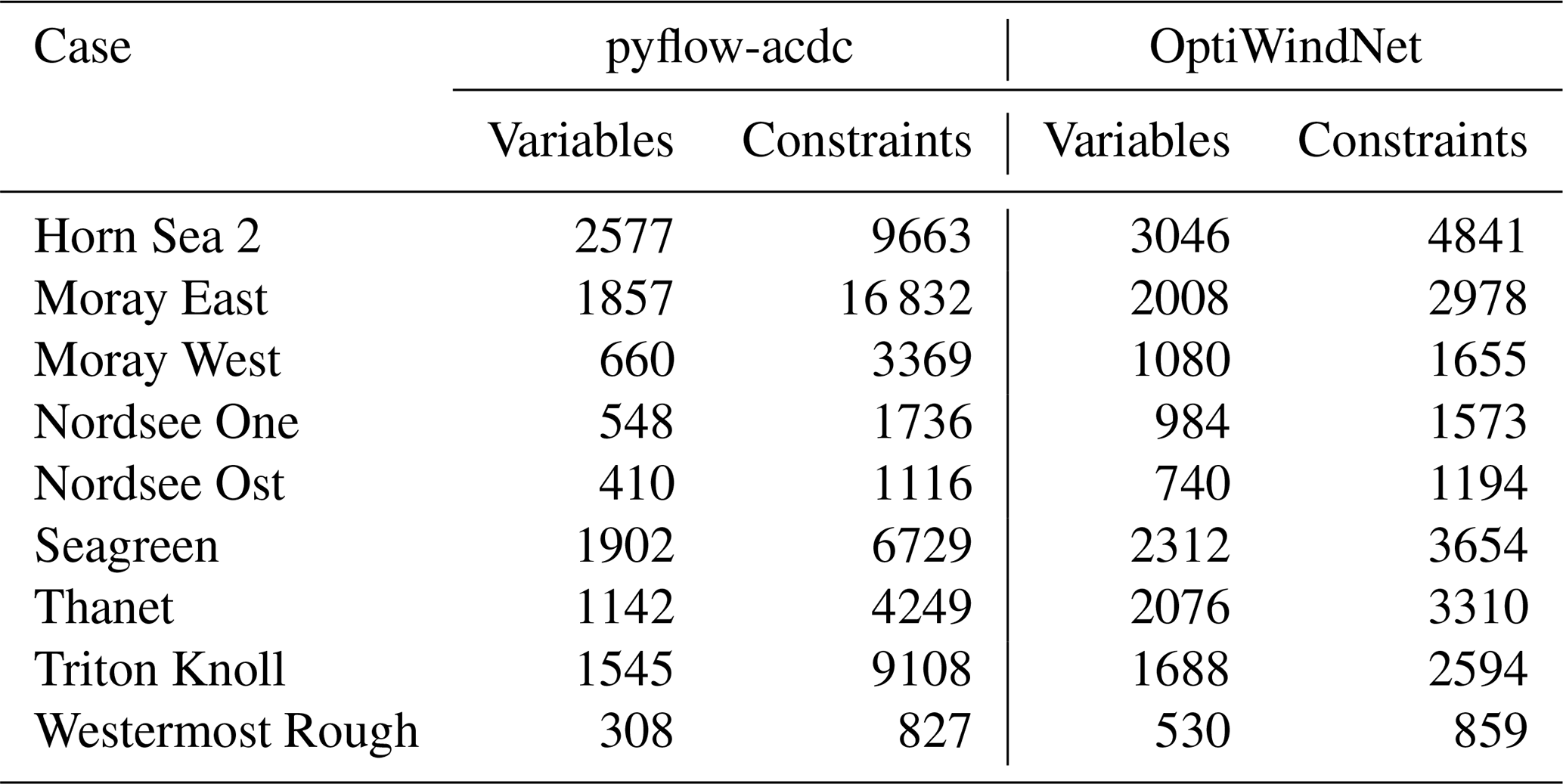
Table 7MILP formulation characteristics and optimisation results for the turbine location test systems.
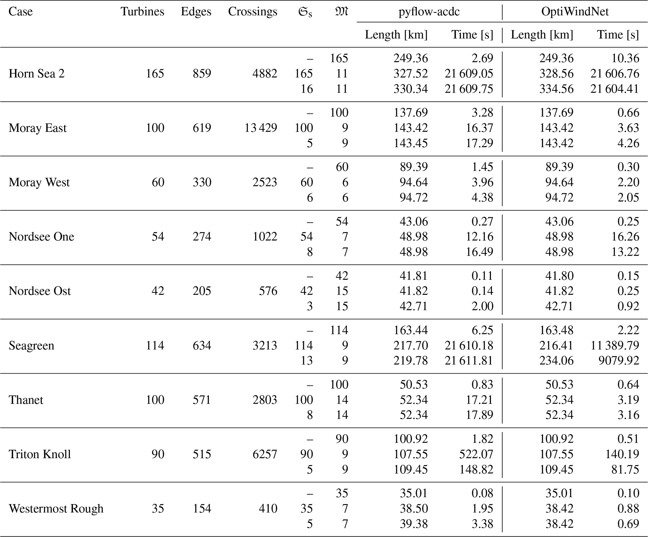
The second evaluation concerns computational performance, shown in Table 7. The proposed methodology is slower in most cases. The explicit modelling of cable crossing restrictions increases the number of constraints and introduces a combinatorial structure that is more difficult for the branch-and-bound algorithm to resolve. Although feasible solutions of comparable quality are identified early in the search, the LP relaxation bound is weaker than that of the planar-embedding approach, making the optimality gap more challenging to close within a given time limit. The advantage of the reduced variable representation is therefore not necessarily a reduction in solution time but a simpler representation of each candidate connection that facilitates the incorporation of additional routing and CSS constraints. This simplification is, however, counterbalanced by the static crossing constraints.
Both methodologies produce comparable routing lengths across the nine wind farms, with larger differences appearing mainly in the more constrained balanced cases. It is worth noting that OptiWindNet's topology-optimisation objective can differ from the final embedded route length when post-processing detours are required. For example, in the third Horn Sea 2 test, the topology-optimisation length before re-routing is 325.87 km; however, post-processing re-routing to avoid physical cable crossings introduces additional cable length, increasing the final embedded route length to 334.56 km.
In contrast, the proposed methodology enforces crossing avoidance directly within the MILP solution. While OptiWindNet resolves many crossing issues through topology-embedding separation and post-optimisation detours, the proposed methodology considers crossing candidate edges explicitly within the optimisation through static crossing constraints.
The case study information used for benchmarking is available in the Zenodo repository (Castro Valerio, 2026a).
7.2 Qualitative benchmarking
The comparison in Table 7 evaluates the routing formulation quantitatively, while several modelling aspects require qualitative positioning. Existing routing formulations already include many of the individual components used here: Delaunay-based pathfinding and GIS obstacle avoidance (Pillai et al., 2015), Steiner-node obstacle detours and practical routing variants (Fischetti and Pisinger, 2018a, b), penalty-based obstacle and boundary treatments (Taylor et al., 2023b), and topology-embedding separation with post-optimisation detours (Souza de Alencar et al., 2025). These approaches differ mainly in where spatial feasibility is imposed: during path generation, through additional graph nodes, as penalty terms, or after topology optimisation. The proposed formulation instead applies routing constraints to candidate routes generated by the graph-preparation stage, so hard exclusions, soft-exclusion weights, clearance constraints, and static crossing constraints are reflected before or within the MILP solve.
The core routing MILP follows standard network-design principles, including edge activation, flow conservation, capacity limits, and crossing constraints. Similar routing structures have been used in wind farm collection-system formulations based on directed arc-pairs representations (Fischetti and Pisinger, 2018a, b; Pérez-Rúa et al., 2020a; Souza de Alencar et al., 2025). As shown in the quantitative benchmark, the distinction of the present core routing formulation is the use of a single activation and flow variable per candidate edge, together with the enforcement of a strict radial topology. The formulation is further extended through constraints on the minimum number of turbines per string, the determination of substation connections under unfavourable GIS constraints, and the possibility of unbalanced substation capacities, thereby expanding the range of user-defined design requirements that can be represented.
For CSS and loss-aware design, Cerveira et al. (2016) and Fischetti and Pisinger (2018a) provide the closest comparison with precomputed loss treatments. Both approaches estimate loss-related costs from the cable type and the number of turbines carried by a segment, while Fischetti and Pisinger (2018a) further include wind-scenario probabilities in the expected loss contribution. This keeps the optimisation tractable, but the loss assigned to each segment is based on local loading assumptions rather than on the full electrical state of the selected network. Consequently, upstream voltage conditions, reactive power flows, cable capacitance effects, and cumulative losses along preceding segments are not explicitly represented. In this paper, the ACOPF-based CSS formulation captures losses within the optimisation by representing voltage magnitudes and angles, as well as the full π model of the cable sections. However, this formulation is computationally demanding. For this reason, the linear CSS formulation is used to enable joint routing–CSS optimisation in both the integrated and sequential approaches, although losses are not included in the linear CSS objective.
The strongest joint routing–CSS benchmark is Wędzik et al. (2016), which integrates network routing optimisation with CSS and includes restrictions on the number of cable cross-sections used. However, coupling CSS with balanced radial-routing constraints introduces an additional difficulty: the routing balance depends on the maximum number of turbines that can be carried by the largest conductor selected, but this conductor is itself an optimisation outcome. If this maximum capacity is fixed in advance, the routing problem can enforce balanced strings more easily, but the conductor-selection problem is partially predetermined. Conversely, if the conductor set is left fully open, the routing formulation cannot directly know which turbine-per-string limits should be imposed to obtain a balanced configuration. The sequential strategy is therefore used to explore this dependency step by step, restricting the available conductor set across iterations and re-solving the routing problem with the corresponding balance and substation-connection constraints. This allows the effect of conductor availability on routing, trenching cost, and CSS cost to be evaluated more explicitly than in a single integrated solution.
7.3 Limitations
In all cases, the routing algorithm is constrained by the graph preparation process. The inclination threshold determines the viability of candidate connections, while soft-exclusion penalties modify their weights and therefore influence their selection. The level of densification further determines the spatial resolution of the graph, where higher densification can provide better-informed candidate paths at the expense of increased computational cost. Connections that may appear feasible upon visual inspection can be excluded due to cable crossing constraints, an inherent limitation of using static constraints. As illustrated in Fig. 12a, a visually preferable routing might involve connecting the leftmost turbine (highlighted in blue) of the orange string directly to the substation, thereby reducing total cable length. However, this configuration is excluded by the algorithm because it intersects with other inter-turbine edges.
In another example, shown in Fig. 12c, the connection set in orange originates from the original project documentation but would be excluded under the current method, as it crosses other active connections. Another restriction concerns the connectivity of possible turbine-to-turbine links. In the methodology proposed in Sect. 2, such connections are defined using Delaunay and diagonal edges. In Fig. 12b, the orange link, also derived from the project documentation, would not be considered under a Delaunay-diagonal configuration. This could be extended, optionally, by incorporating k-nearest neighbours into the search; however, doing so increases the graph preparation time and complicates the routing problem.
Moreover, under the graph preparation procedure, connections originating from the substation and overlapping with other substation links are not classified as crossings by the algorithm. Consequently, multiple such connections are permitted. This is also visible in Fig. 12a, where area constraints result in parallel segments running from the substation to different turbines. These examples underscore the importance not only of careful graph preparation but also of incorporating human oversight to mitigate limitations inherent in automated routing strategies.
Some of the limitations discussed above could be alleviated by refining the candidate-edge construction. Additional Steiner points, as used in related routing studies, could be introduced to increase the number of feasible detours and reduce the restrictive effect of static crossing constraints. In the limiting case, the routing optimisation could be performed directly on the densified graph produced during graph preparation step (d), rather than on the reduced candidate graph. This would provide greater routing flexibility but would substantially increase the number of candidate edges and crossing constraints. A practical compromise is therefore to adjust the density of the graph-preparation stage according to the size and complexity of the test case. Higher densification improves the spatial resolution of the three-dimensional path assessment but also increases the computational cost of pathfinding and subsequent routing optimisation.
The MILP scalability is mainly limited by the explicit crossing constraints. These constraints increase with the number of intersecting candidate-edge pairs and can make it difficult for the solver to close the optimality gap, particularly in larger or more constrained cases. The optimality gap is the difference between the best feasible solution and the solver's lower bound, which is obtained from LP relaxations and provides a provable bound on the optimal objective (Gurobi Optimization, LLC, 2026).
In the linear CSS formulations, losses are not included in the objective in order to keep the routing–CSS problem linear and computationally tractable. Loss-related terms could be incorporated through precomputed coefficients, as in previous loss-aware routing formulations, but such an extension would require assumptions on segment loading and would not represent the full AC state of the selected network. For this reason, losses are instead evaluated through the separate non-linear CSS formulation.
The non-linear formulation is evaluated using an equivalent full-load-hours analysis, which represents the annual operation of the wind farm by a single operating point. Consequently, the optimisation does not capture the variation in active and reactive power flows under different operating conditions. In particular, it does not account for the increased relative contribution of cable charging losses at lower loading conditions, especially for oversized conductors with higher capacitance (Dakic et al., 2021). A more detailed representation could be obtained through a multi-scenario approach, as presented in Valerio et al. (2026a), in which the wind speed Weibull distribution and turbine power curve are used to generate representative operating scenarios, each associated with a probability. Similarly, time series data can be clustered into representative operating conditions to capture spatial and temporal variations in turbine production. The main limitation of these approaches is the substantially increased computational burden, as the optimisation must be solved simultaneously for multiple operating scenarios rather than a single equivalent operating point.
This paper presents a set of stages for the optimisation of inter-array grids in wind parks. Each stage may be applied independently to enhance existing workflows or combined into either an integrated or sequential algorithm, both of which are also introduced in this work. The first stage configures the graph representation of turbine and substation interconnections, taking into account bathymetry or elevation, inclination thresholds, export cables, and both soft- and hard-exclusion zones. The second stage introduces a core model to optimise a radial array, constraining bifurcations, crossings, and the number of turbines per string through the formulation of a mixed-integer problem. This model can be extended to accommodate a minimum number of turbines per string, determine the minimum number of substation connections required, or incorporate substations with different power capacities. The third stage addresses conductor size selection, limiting the number of selected conductors by employing a DC linear approximation of the power flow.
The second and third stages may be iterated within an integrated algorithm to solve the problem simultaneously or within a sequential algorithm to identify the optimal trade-off between the maximum number of turbines per string and conductor investment. These two approaches are compared across more than 30 case studies, in which the sequential approach further restricts the problem to enable the generation of routes that are both technically feasible and electrically balanced.
The case studies are based on existing turbine ratings and locations, encompassing both onshore and offshore scenarios. While they demonstrate the strategies' usability, they cannot be directly compared to real project deployments, as the input data used by the authors differ from those of the individual projects. In addition, the quantitative benchmarking is mainly focused on the routing stage, with the complete framework assessed through its application to the case studies. These aspects limit the extent to which its overall performance can be compared against existing approaches. In the case of the Moray developments, where a realistic representation of cable paths was publicly available, the optimisation predicted a very similar interconnection routing.
The benchmarking further shows that the proposed routing formulation provides comparable routing lengths to an open-source reference framework while reducing the number of routing variables through a single representation for each candidate edge. This comes at the cost of additional crossing constraints, which can make it more difficult to close the optimality gap in larger or more spatially constrained cases. The qualitative comparison further indicates that, although the individual modelling components are based on existing concepts, they have been adapted to address the requirements of the proposed workflow. The principal contribution of this work therefore lies in integrating these components into a joint graph-preparation, routing, and CSS framework that accounts simultaneously for realistic spatial constraints, user-defined routing requirements, and conductor type restrictions.
Although the use of mixed-integer linear programming for joint routing and conductor sizing, either in an integrated formulation or in a sequential approach with linear or non-linear CSS, increases computational complexity relative to greedy heuristics, it provides a structured framework capable of addressing increasingly complex constraints encountered in real-world wind farm developments that are often overlooked in simpler models. However, the quality of the final routing remains sensitive to the granularity and accuracy of the graph preparation stage. As such, the approach is conceived as a planning support tool that aids the human design process, particularly in navigating complex physical and operational constraints.
A1 Sets and indices
| 𝒩ac | Set of all nodes in the network |
| 𝒩t | Set of turbine nodes |
| 𝒩s | Set of substation nodes |
| ℰ | Set of candidate edges |
| ℰi | Set of edges connected to node i |
| 𝒜 | Set of active edges selected by the routing stage |
| ℐ | Set of available conductor types |
| i,k | Indices of network nodes |
| Edge-connecting nodes i and k | |
| ι | Index of conductor type |
| ℱ | Feasible solution set |
A2 Decision variables
| ξa | Binary variable indicating whether edge a is active |
| ξa,ι | Binary variable indicating assignment of conductor type ι to edge a |
| νι | Binary variable indicating whether conductor type ι is used |
| fa | Integer power flow on edge a |
| za,ι | Auxiliary variable for McCormick linearisation |
| Largest conductor type that was assigned |
A3 Routing design parameters
| pi | Net power injection at node i |
| 𝔐 | Maximum number of turbines per string |
| 𝔪 | Minimum number of turbines per string |
| 𝔰s | Minimum number of string connections per substation |
| 𝔖s | Maximum number of connections per substation |
| 𝔐ι | Flow capacity of conductor type ι |
| 𝔑 | Maximum number of conductor types allowed |
| 𝒲a | Weighted length of edge a |
| La | Geometric length of edge a |
| ψa | Installation cost per unit of weighted length |
| ψι | Cost per unit of length of conductor type ι |
A4 Electrical quantities
| Vi | Voltage magnitude at node i |
| θi | Voltage angle at node i |
| Pik,Qik | Active and reactive power flow from node i to node k |
| Sik | Apparent power flow from node i to node k |
| Apparent power flow on branch a using conductor type ι | |
| Active and reactive turbine power at node i | |
| Active and reactive substation power at node i | |
| Curtailment factor at turbine node i | |
| Ma | Big-M parameter for branch a |
| κ | Security factor for Ma |
A5 Economic parameters
| α | Weighting parameter in the multi-objective function |
| r | Discount rate |
| y | Project lifetime (years) |
| Hy | Full-load hours over y years |
| ρ | Electricity cost |
This appendix provides detailed information on the test cases and their corresponding results. Table B1 summarises the specific characteristics of each case.
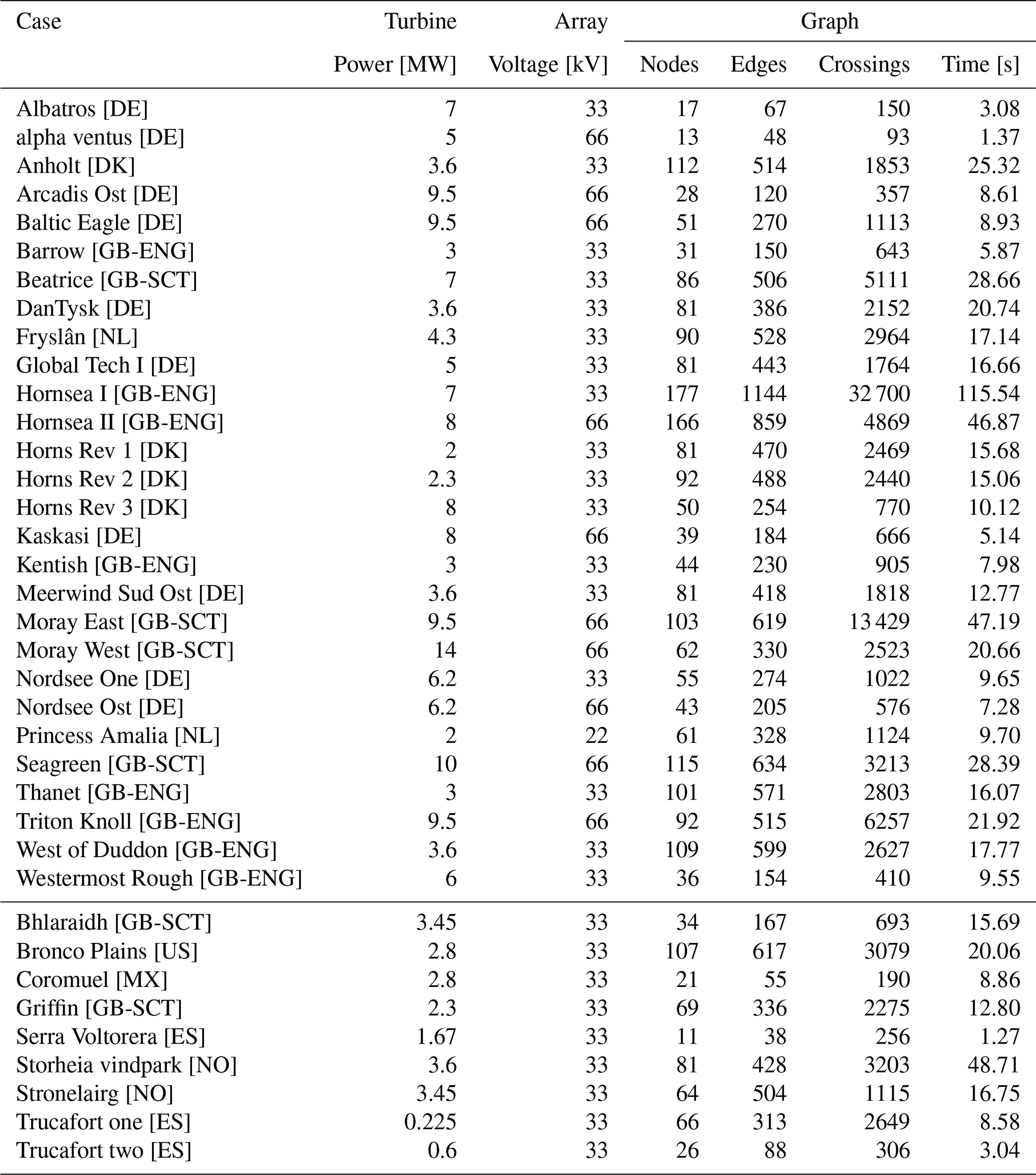
This appendix provides information on the conductor sets used in the test cases. The cable data are compiled from ABB (2010a) for onshore cables and ABB (2010b) for offshore submarine cables. In all simulations, the cost per metre of each conductor is estimated as
taken from Dicorato et al. (2011), where S denotes the conductor cross-sectional area. In this approximation, neither the voltage level nor the conductor material is explicitly considered. Consequently, the resulting cost values are employed solely for methodology validation within the presented case studies and should not be interpreted as industrial quotations, project-specific estimates, or commercially validated cable prices.
For onshore 33 kV cables in Table C1, reference ABB (2010a) does not provide data directly; therefore, the corresponding values were extrapolated from the available voltage levels. For the conductors used in the non-linear CSS in Table C6, the cable parameters are taken from the ABB dataset, whereas the cable capacities are taken from Marine Scotland (2019, 2022).
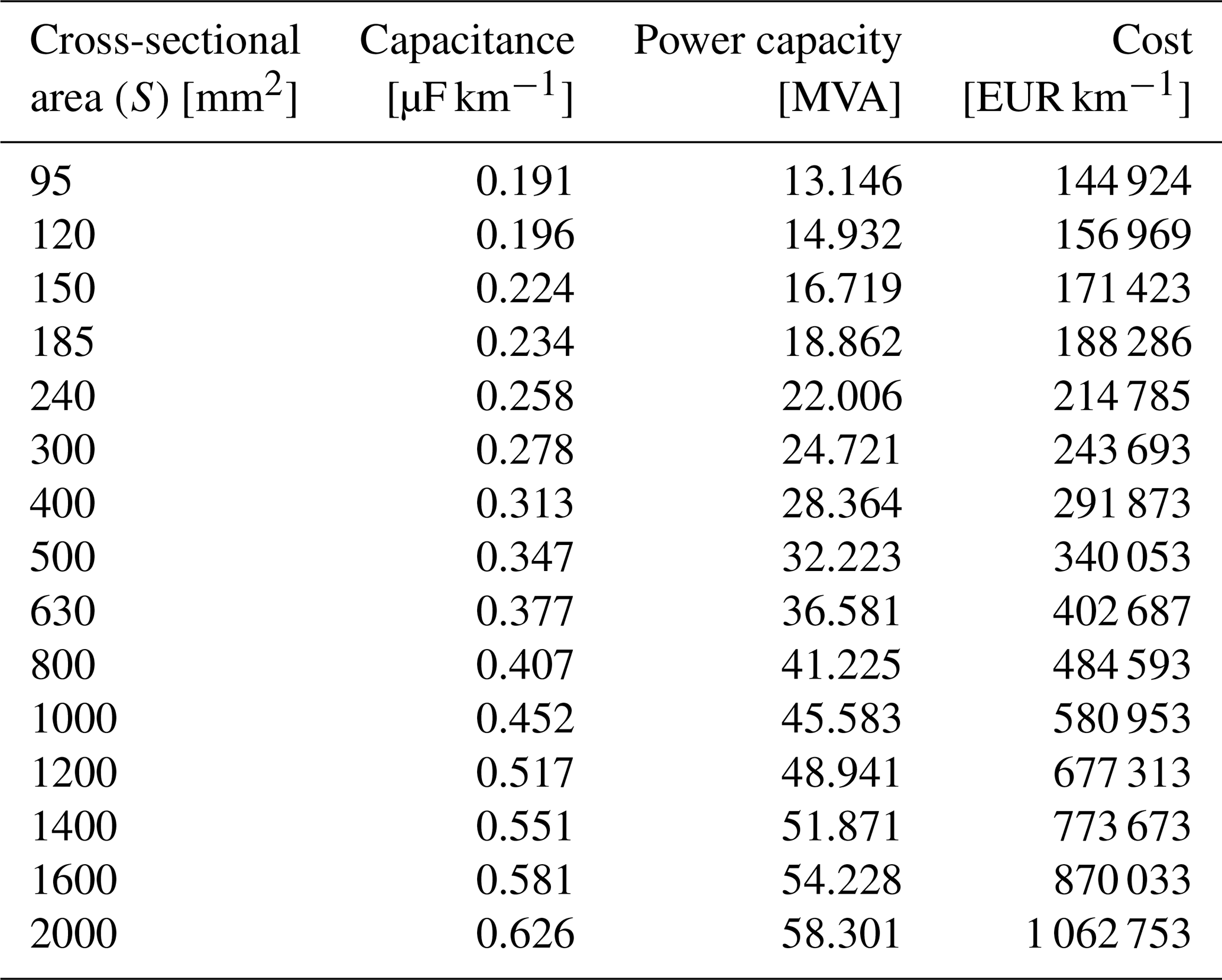
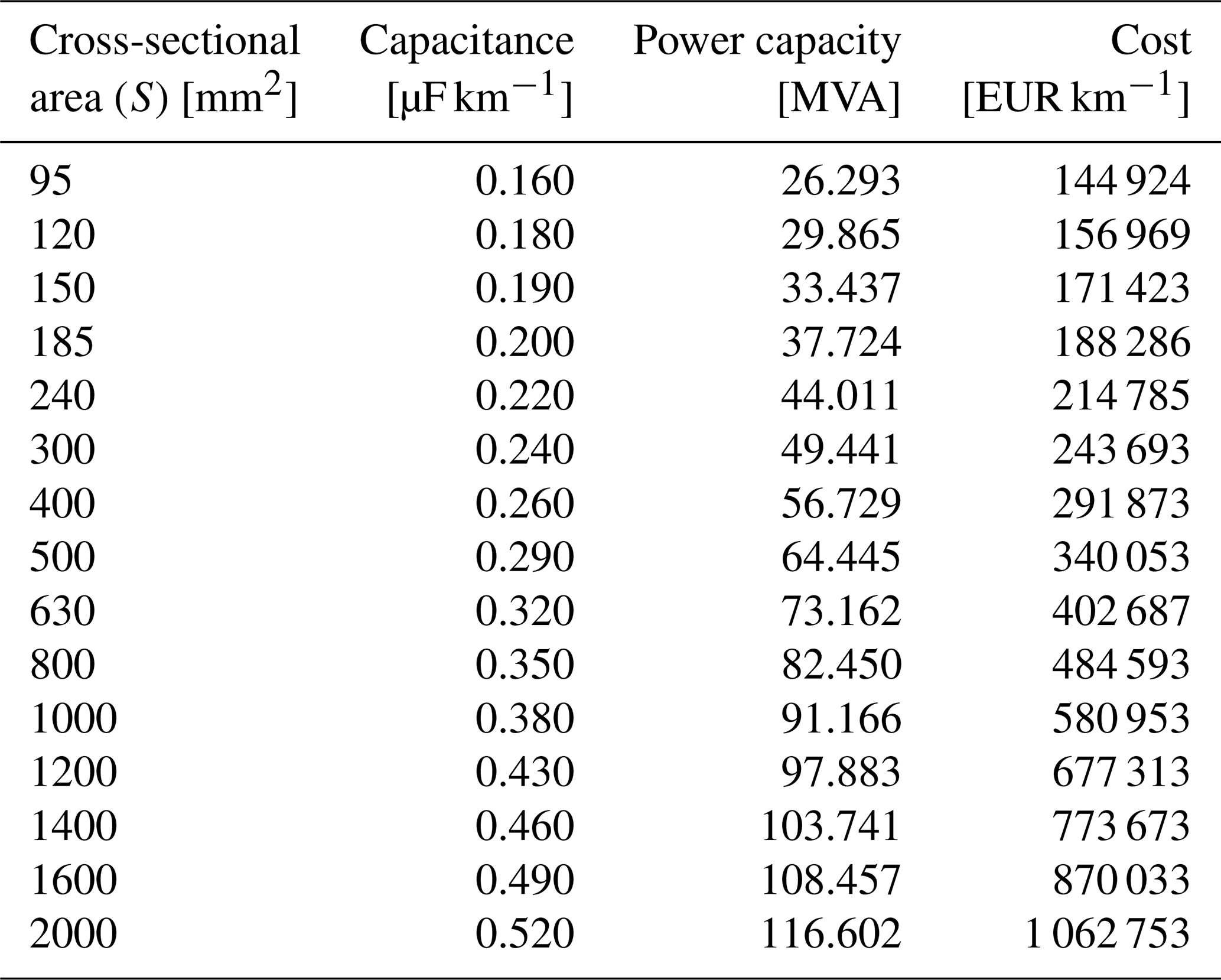
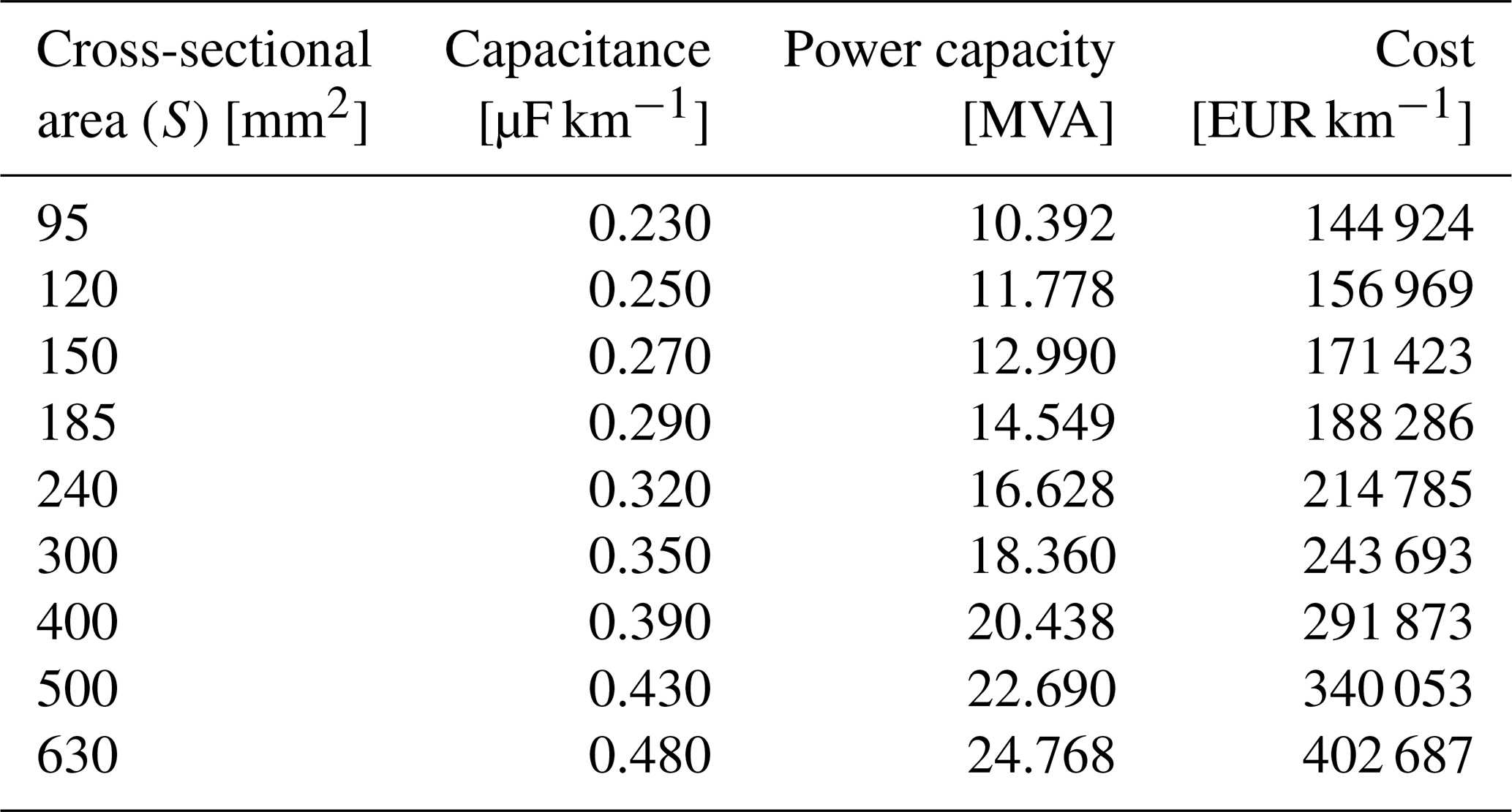
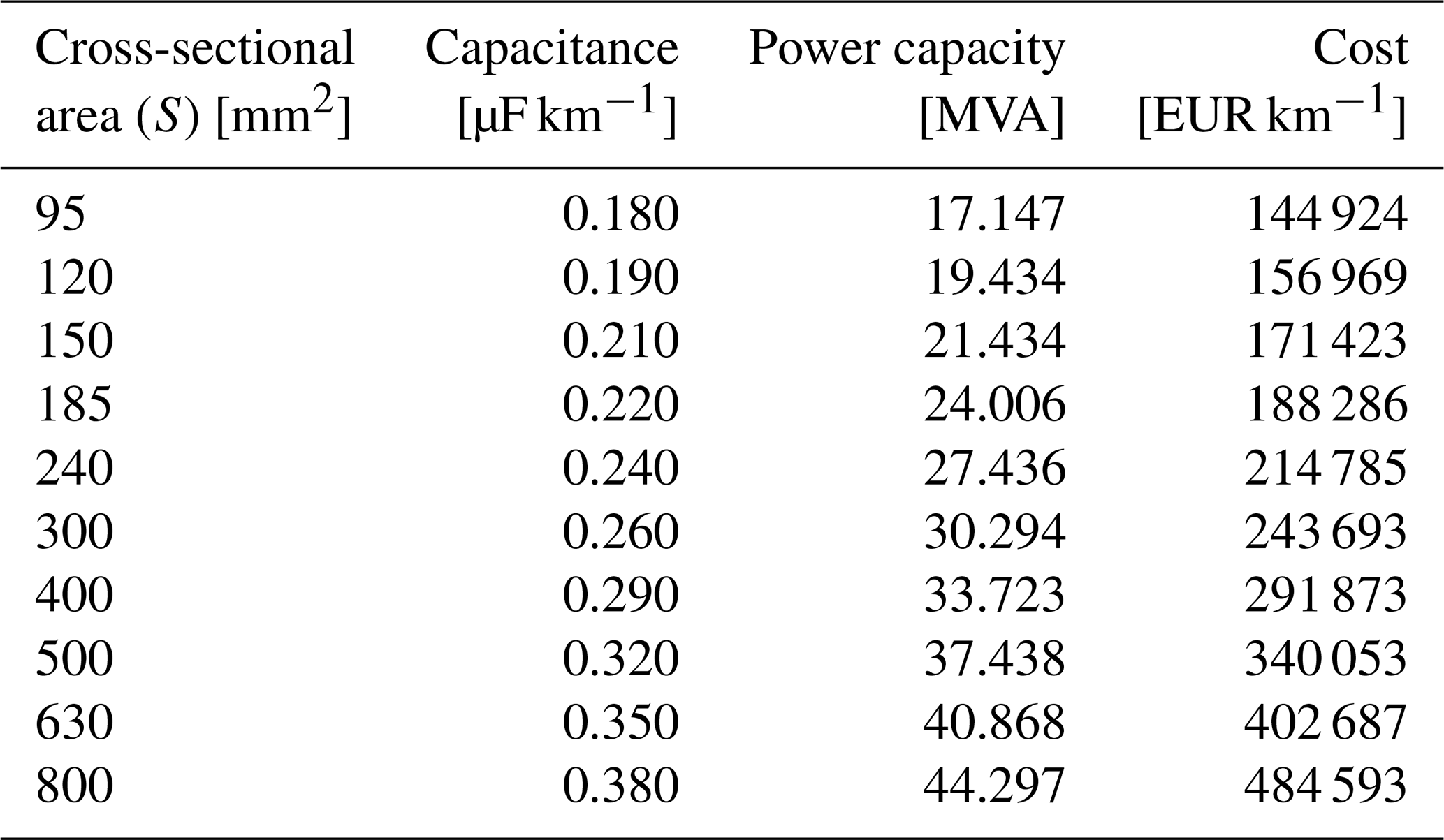
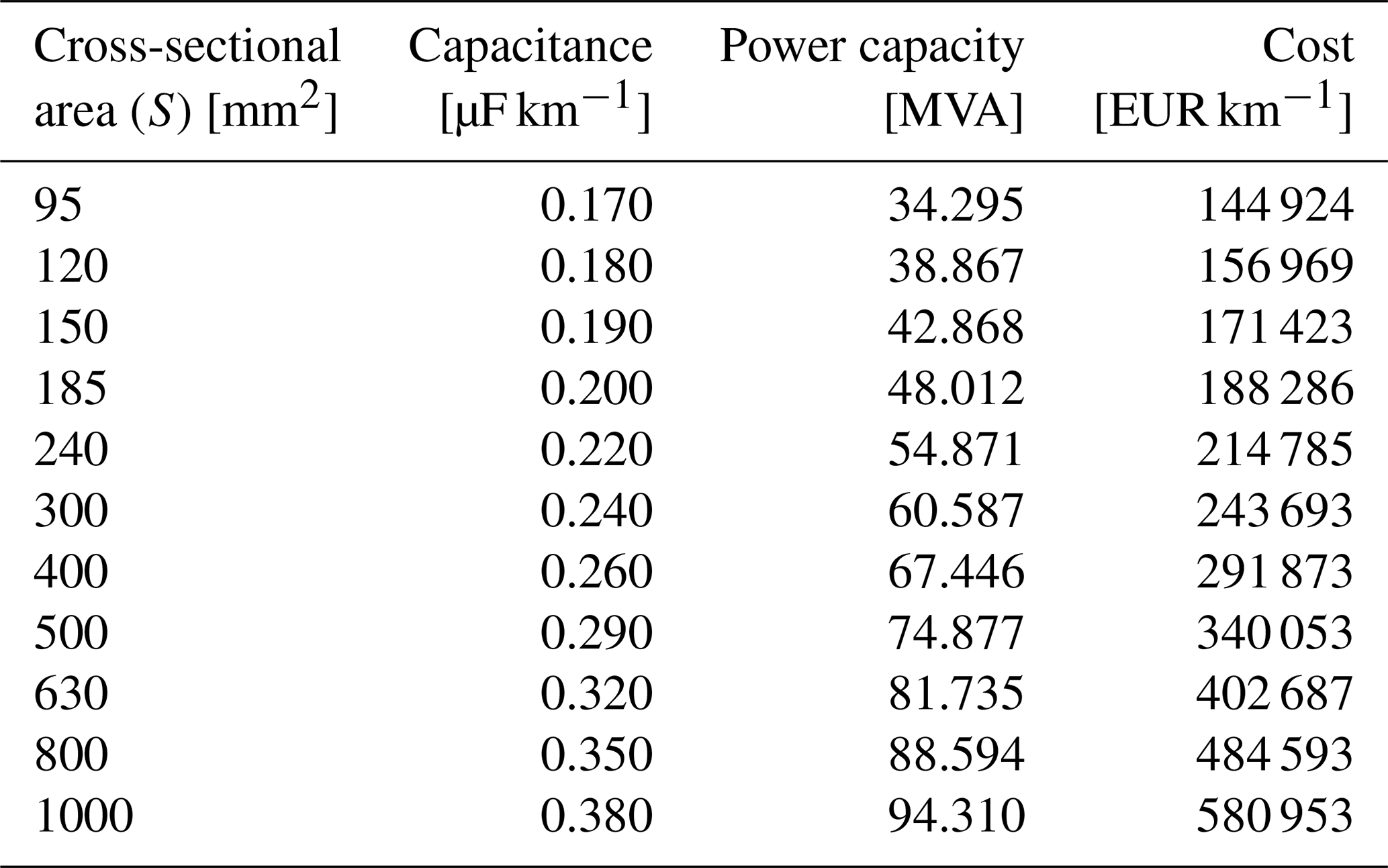
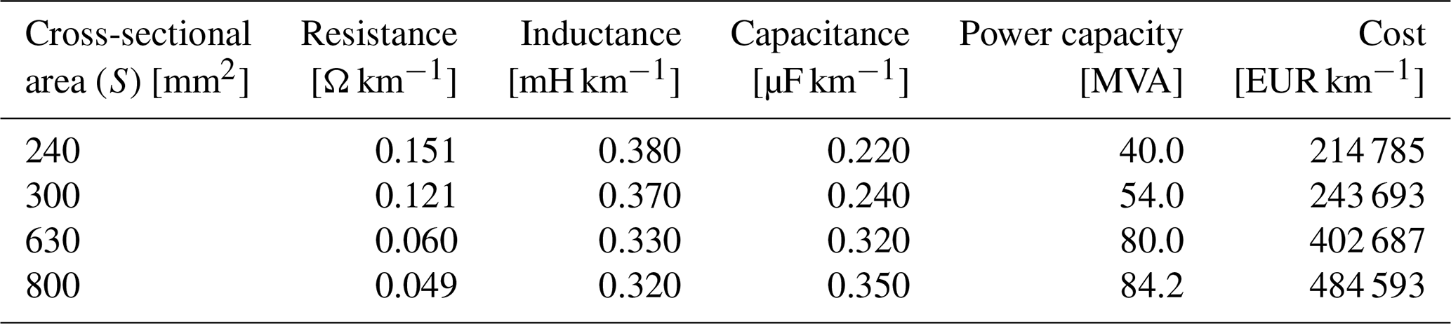
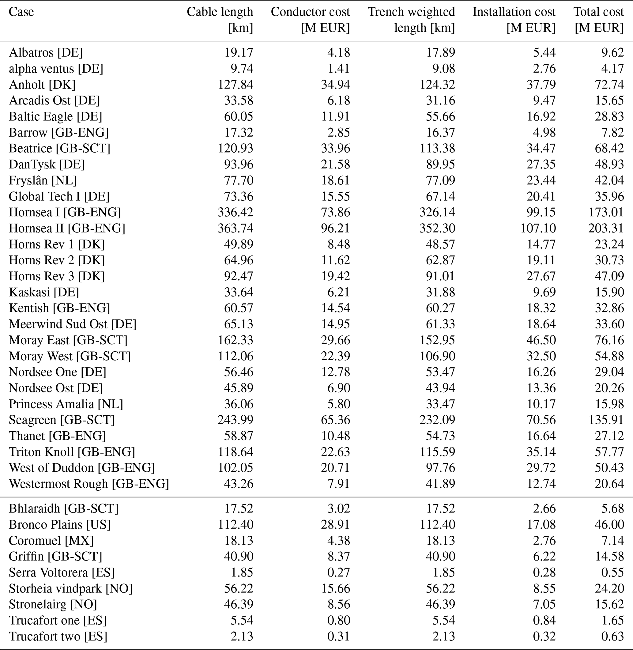
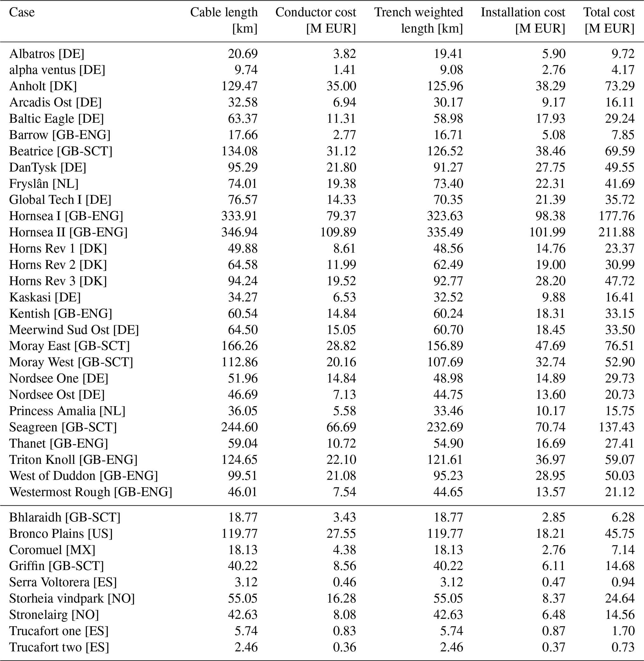
Code for the optimisation is available as part of the pyflow-acdc v0.5.1 (Valerio et al., 2025) Python package. The data and code used to run all case studies are presented in Castro Valerio (2026b).
Bernardo Castro Valerio: Writing – original draft and review and editing, Conceptualisation, Data curation, Formal analysis, Methodology, Software, Validation, Visualisation. Pieter Gebraad: Data curation, Writing review and editing, Funding acquisition, Supervision. Marc Cheah-Mane: Writing review and editing, Funding acquisition, Supervision. Vinicius Lacerda: Writing review and editing, Funding acquisition, Project administration, Supervision. Oriol Gomis-Bellmunt: Writing review and editing, Funding acquisition, Project administration, Supervision.
The contact author has declared that none of the authors has any competing interests.
Publisher's note: Copernicus Publications remains neutral with regard to jurisdictional claims made in the text, published maps, institutional affiliations, or any other geographical representation in this paper. The authors bear the ultimate responsibility for providing appropriate place names. Views expressed in the text are those of the authors and do not necessarily reflect the views of the publisher.
During the preparation of this work, the authors used GPT-4o and GPT-5 in order to improve grammar and language readability. After using this tool/service, the authors reviewed and edited the content as needed and take full responsibility for the content of the publication.
This work has received funding from the ADOreD project of the European Union’s Horizon Europe Research and Innovation programme under the Marie Skłodowska-Curie Actions (grant no. 101073554).
This paper was edited by Nicolaos A. Cutululis and reviewed by three anonymous referees.
ABB: XLPE Land Cable Systems: User's Guide, ABB, rev. 5 edn., 2010a. a, b, c
ABB: XLPE Submarine Cable Systems: Attachment to XLPE Land Cable Systems – User's Guide, ABB, rev. 5 edn., https://new.abb.com/docs/default-source/ewea-doc/xlpe-submarine-cable-systems-2gm5007.pdf (last access: 18 September 2026), 2010b. a, b, c
Bae, I.-S., Son, E.-T., Kim, S.-Y., and Kim, D.-M.: Optimum Cable Sizing for Offshore Wind Farms Using Binary Integer Programming, IEEE Access, 11, 132708–132717, https://doi.org/10.1109/ACCESS.2023.3336163, 2023. a
BGV Associates: Wind Farm Costs, https://guidetoanoffshorewindfarm.com/wind-farm-costs/ (last access: 18 September 2026), 2025. a
Bonami, P., Biegler, L. T., Conn, A. R., Cornuéjols, G., Grossmann, I. E., Laird, C. D., Lee, J., Lodi, A., Margot, F., Sawaya, N., and Wächter, A.: An algorithmic framework for convex mixed integer nonlinear programs, Discrete Optimization, 5, 186–204, https://doi.org/10.1016/j.disopt.2006.10.011, 2008. a
Castro Valerio, B.: Code and examples for running benchmarking inter-array models of wind farms, Zenodo, https://doi.org/10.5281/zenodo.18846347, 2026a. a
Castro Valerio, B.: Code and data for Case Studies of: A multi-stage methodology for wind park inter-array cabling: graph preparation, layout, and sizing, Zenodo [data set], https://doi.org/10.5281/zenodo.18937430, 2026b. a
Cazzaro, D. and Pisinger, D.: Balanced cable routing for offshore wind farms with obstacles, Networks, 80, 386–406, https://doi.org/10.1002/net.22100, 2022. a
Cazzaro, D., Fischetti, M., and Fischetti, M.: Heuristic algorithms for the Wind Farm Cable Routing problem, Appl. Energ., 278, 115617, https://doi.org/10.1016/j.apenergy.2020.115617, 2020. a
Cerveira, A., de Sousa, A., Pires, E. J. S., and Baptista, J.: Optimal Cable Design of Wind Farms: The Infrastructure and Losses Cost Minimization Case, IEEE T. Power Syst., 31, 4319–4329, https://doi.org/10.1109/TPWRS.2016.2521700, 2016. a, b
Chen, Y., Dong, Z. Y., Meng, K., Luo, F., Xu, Z., and Wong, K. P.: Collector System Layout Optimization Framework for Large-Scale Offshore Wind Farms, IEEE T. Sustain. Energ., 7, 1398–1407, https://doi.org/10.1109/TSTE.2016.2549602, 2016. a, b
Dakic, J., Cheah-Mane, M., Gomis-Bellmunt, O., and Prieto-Araujo, E.: HVAC Transmission System for Offshore Wind Power Plants Including Mid-Cable Reactive Power Compensation: Optimal Design and Comparison to VSC-HVDC Transmission, IEEE T. Power Deliver., 36, 2814–2824, https://doi.org/10.1109/TPWRD.2020.3027356, 2021. a
Dicorato, M., Forte, G., Pisani, M., and Trovato, M.: Guidelines for assessment of investment cost for offshore wind generation, Renew. Energ., 36, 2043–2051, https://doi.org/10.1016/j.renene.2011.01.003, 2011. a, b, c
Dutta, S. and Overbye, T. J.: Optimal Wind Farm Collector System Topology Design Considering Total Trenching Length, IEEE T. Sustain. Energ., 3, 339–348, https://doi.org/10.1109/TSTE.2012.2185817, 2012. a
El Mokhi, C. and Addaim, A.: Optimal Substation Location Of A Wind Farm Using Different Metaheuristic Algorithms, in: 2020 IEEE 6th International Conference on Optimization and Applications (ICOA), 1–6, https://doi.org/10.1109/ICOA49421.2020.9094469, 2020. a
Fischetti, M. and Pisinger, D.: Optimizing wind farm cable routing considering power losses, Eur. J. Oper. Res., 270, 917–930, https://doi.org/10.1016/j.ejor.2017.07.061, 2018a. a, b, c, d, e, f, g, h, i, j
Fischetti, M. and Pisinger, D.: Optimal wind farm cable routing: Modeling branches and offshore transformer modules, Networks, 72, 42–59, https://doi.org/10.1002/net.21804, 2018b. a, b, c, d, e, f, g
GEBCO Bathymetric Compilation Group: The GEBCO_2025 Grid – a continuous terrain model for oceans and land at 15 arc-second intervals, NERC EDS British Oceanographic Data Centre, NOC, https://doi.org/10.5285/37c52e96-24ea-67ce-e063-7086abc05f29, 2025. a
Gong, X., Kuenzel, S., and Pal, B. C.: Optimal Wind Farm Cabling, IEEE T. Sustain. Energ., 9, 1126–1136, https://doi.org/10.1109/TSTE.2017.2771147, 2018. a, b
Gurobi Optimization, LLC: Gurobi Optimizer Reference Manual, https://www.gurobi.com (last access: 18 September 2026), 2026. a, b, c
Hagberg, A. A., Schult, D. A., and Swart, P. J.: Exploring Network Structure, Dynamics, and Function using NetworkX, Python in Science Conference, https://doi.org/10.25080/TCWV9851, 2008. a, b
Hou, P., Hu, W., Chen, C., and Chen, Z.: Overall Optimization for Offshore Wind Farm Electrical System, Wind Energy, 20, https://doi.org/10.1002/we.2077, 2016. a
Hou, P., Zhu, J., Ma, K., Yang, G., Hu, W., and Chen, Z.: A review of offshore wind farm layout optimization and electrical system design methods, J. Mod. Power Syst. Cle., 7, 975–986, https://doi.org/10.1007/s40565-019-0550-5, 2019. a
Kallinger, M. D., Rapha, J. I., Trubat Casal, P., and Domínguez-García, J. L.: Offshore Electrical Grid Layout Optimization for Floating Wind – A Review, Clean Technologies, 5, 791–827, https://doi.org/10.3390/cleantechnol5030039, 2023. a
Kost, C., Müller, P., Sepulveda Schweiger, J., Fluri, V., and Thomsen, J.: Levelized Cost of Electricity of Renewable Energy Technologies, Tech. rep., Fraunhofer Institute for Solar Energy Systems ISE, https://www.ise.fraunhofer.de/en/publications/studies/cost-of-electricity.html (last access: 18 September 2026), 2024. a
Lumbreras, S. and Ramos, A.: Optimal Design of the Electrical Layout of an Offshore Wind Farm Applying Decomposition Strategies, IEEE T. Power Syst., 28, 1434–1441, https://doi.org/10.1109/TPWRS.2012.2204906, 2013. a
Marine Scotland: Moray East Offshore Windfarm – Cable Plan, Tech. rep., Marine Scotland, https://marine.gov.scot/?q=data/moray-east-offshore-windfarm-cable-plan (last access: 18 September 2026), 2019. a, b, c, d
Marine Scotland: Moray West Inter Array Cable Plan, Tech. rep., Marine Scotland, https://marine.gov.scot/?q=node/23687 (last access: 18 September 2026), 2022. a, b, c, d
Moon, W.-S., Kim, J.-C., Jo, A., and Won, J.-N.: Grid optimization for offshore wind farm layout and substation location, in: 2014 IEEE Conference and Expo Transportation Electrification Asia-Pacific (ITEC Asia-Pacific), 1–6, https://doi.org/10.1109/ITEC-AP.2014.6941124, 2014. a
Pérez-Rúa, J.-A. and Cutululis, N. A.: Electrical Cable Optimization in Offshore Wind Farms – A Review, IEEE Access, 7, 85796–85811, https://doi.org/10.1109/ACCESS.2019.2925873, 2019. a, b
Pérez-Rúa, J.-A., Stolpe, M., and Cutululis, N. A.: Integrated Global Optimization Model for Electrical Cables in Offshore Wind Farms, IEEE T. Sustain. Energ., 11, 1965–1974, https://doi.org/10.1109/TSTE.2019.2948118, 2020a. a, b, c, d, e, f, g
Pérez-Rúa, J.-A., Stolpe, M., Das, K., and Cutululis, N. A.: Global Optimization of Offshore Wind Farm Collection Systems, IEEE T. Power Syst., 35, 2256–2267, https://doi.org/10.1109/TPWRS.2019.2957312, 2020b. a
Perron, L. and Furnon, V.: OR-Tools, https://developers.google.com/optimization/ (last access: 18 September 2026), 2025. a
Pillai, A., Chick, J., Johanning, L., Khorasanchi, M., and de Laleu, V.: Offshore wind farm electrical cable layout optimization, Eng. Optimiz., 47, 1689–1708, https://doi.org/10.1080/0305215X.2014.992892, 2015. a, b, c, d
Qi, Y., Hou, P., Yang, L., and Yang, G.: Simultaneous Optimisation of Cable Connection Schemes and Capacity for Offshore Wind Farms via a Modified Bat Algorithm, Appl. Sci., 9, 265, https://doi.org/10.3390/app9020265, 2019. a
Rentschler, M. U., Adam, F., and Chainho, P.: Design optimization of dynamic inter-array cable systems for floating offshore wind turbines, Renew. Sust. Energ. Rev., 111, 622–635, https://doi.org/10.1016/j.rser.2019.05.024, 2019. a
Sedighi, M., Moradzadeh, M., Kukrer, O., and Fahrioglu, M.: Simultaneous optimization of electrical interconnection configuration and cable sizing in offshore wind farms, J. Mod. Power Syst. Cle., 6, 749–762, https://doi.org/10.1007/s40565-017-0366-0, 2018. a, b
Serrano González, J., Burgos Payán, M., Santos, J. M. R., and González-Longatt, F.: A review and recent developments in the optimal wind-turbine micro-siting problem, Renew. Sust. Energ. Rev., 30, 133–144, https://doi.org/10.1016/j.rser.2013.09.027, 2014. a
Smail, H., Alkama, R., and Medjdoub, A.: Optimal design of the electric connection of a wind farm, Energy, 165, 972–983, https://doi.org/10.1016/j.energy.2018.10.015, 2018. a, b
Souza de Alencar, M., Göçmen, T., and Cutululis, N. A.: Flexible cable routing framework for wind farm collection system optimization, Eur. J. Oper. Res., https://doi.org/10.1016/j.ejor.2025.07.069, 2025. a, b, c, d, e, f
Taylor, P., Yue, H., Campos-Gaona, D., Anaya-Lara, O., and Jia, C.: Wind farm array cable layout optimisation for complex offshore sites – A decomposition based heuristic approach, IET Renew. Power Gen., 17, 243–259, https://doi.org/10.1049/rpg2.12593, 2023a. a
Taylor, P., Yue, H., Campos-Gaona, D., Anaya-Lara, O., and Jia, C.: Wind farm array cable layout optimisation for complex offshore sites – A decomposition based heuristic approach, IET Renew. Power Gen., 17, 243–259, https://doi.org/10.1049/rpg2.12593, 2023b. a, b, c, d
Ulku, I. and Alabas-Uslu, C.: Optimization of cable layout designs for large offshore wind farms, International Journal of Energy Research, 44, 6297–6312, https://doi.org/10.1002/er.5336, 2020. a
Valerio, B. C., Lacerda, V. A., Cheah-Mane, M., Gebraad, P., and Gomis-Bellmunt, O.: An optimal power flow tool for AC/DC systems, applied to the analysis of the North Sea Grid for offshore wind integration, IEEE T. Power Syst. [code], 1–14, https://doi.org/10.1109/TPWRS.2025.3533889, 2025. a, b
Valerio, B. C., Cheah-Mane, M., Lacerda, V. A., Gebraad, P., and Gomis-Bellmunt, O.: Transmission expansion planning for hybrid AC/DC grids using a mixed-integer non-linear programming approach, Int. J. Elec. Power, 174, 111459, https://doi.org/10.1016/j.ijepes.2025.111459, 2026a. a, b
Valerio, B. C., Gebraad, P. M., Cheah-Mane, M., Lacerda, V., and Gomis-Bellmunt, O.: Strategies for wind park inter array optimisation through Mixed Integer Linear Programming, J. Phys. Conf. Ser., 3224, 052005, https://doi.org/10.1088/1742-6596/3224/5/052005, 2026b. a
Virtanen, P., Gommers, R., Oliphant, T. E., Haberland, M., Reddy, T., Cournapeau, D., Burovski, E., Peterson, P., Weckesser, W., Bright, J., van der Walt, S. J., Brett, M., Wilson, J., Millman, K. J., Mayorov, N., Nelson, A. R. J., Jones, E., Kern, R., Larson, E., Carey, C. J., Polat, İ., Feng, Y., Moore, E. W., VanderPlas, J., Laxalde, D., Perktold, J., Cimrman, R., Henriksen, I., Quintero, E. A., Harris, C. R., Archibald, A. M., Ribeiro, A. H., Pedregosa, F., van Mulbregt, P., and SciPy 1.0 Contributors: SciPy 1.0: Fundamental Algorithms for Scientific Computing in Python, Nat. Methods, 17, 261–272, https://doi.org/10.1038/s41592-019-0686-2, 2020. a
Wędzik, A., Siewierski, T., and Szypowski, M.: A new method for simultaneous optimizing of wind farm’s network layout and cable cross-sections by MILP optimization, Appl. Energ., 182, 525–538, https://doi.org/10.1016/j.apenergy.2016.08.094, 2016. a, b, c
Wei, S., Zhang, L., Xu, Y., Fu, Y., and Li, F.: Hierarchical Optimization for the Double-Sided Ring Structure of the Collector System Planning of Large Offshore Wind Farms, IEEE T. Sustain. Energ., 8, 1029–1039, https://doi.org/10.1109/TSTE.2016.2646061, 2017. a, b
- Abstract
- Introduction
- Graph preparation
- Collector-system routing
- Conductor size selection
- Joint routing and conductor size optimisation
- Case studies
- Discussion
- Conclusions
- Appendix A: List of symbols
- Appendix B: Case information
- Appendix C: Conductor dataset
- Appendix D: Detailed results
- Code and data availability
- Author contributions
- Competing interests
- Disclaimer
- Acknowledgements
- Financial support
- Review statement
- References
- Abstract
- Introduction
- Graph preparation
- Collector-system routing
- Conductor size selection
- Joint routing and conductor size optimisation
- Case studies
- Discussion
- Conclusions
- Appendix A: List of symbols
- Appendix B: Case information
- Appendix C: Conductor dataset
- Appendix D: Detailed results
- Code and data availability
- Author contributions
- Competing interests
- Disclaimer
- Acknowledgements
- Financial support
- Review statement
- References