Wind turbine wake dynamics subjected to atmospheric gravity waves: a measurement-driven large-eddy simulation study

Atmospheric gravity waves (AGWs) are large-scale wave-like flow structures commonly generated when atmospheric flows are vertically perturbed by topographical features or meteorological phenomena. These transient phenomena can significantly affect wind turbine outputs and loads; however, their influence on wake dynamics remains poorly understood, posing challenges for accurate wind farm modeling. In this study, we perform large-eddy simulation of wind turbines operating under an atmospheric condition reconstructed by assimilating lidar measurements of AGWs. Our results show that (i) low-frequency wake meandering becomes more pronounced owing to large-scale AGW flow structures and intensified smaller-scale turbulent structures. This enhanced meandering, combined with stronger turbulent mixing, accelerates mean wake recovery. (ii) The turbulence kinetic energy (TKE) spectrum in the wake region exhibits a peak Strouhal number of approximately 0.3, although the inflow spectrum peaks at significantly lower frequencies. This observation indicates that, under AGW conditions, wake turbulence generation follows a convective instability mechanism. Notably, faster wake recovery reduces wake shear, leading to lower amplification of TKE. Power analysis for two turbines arranged in a streamwise column further highlights the dominant role of convective instabilities. Large-amplitude, low-frequency power fluctuations observed at the most upstream turbine are significantly attenuated for downstream turbines as low-frequency velocity fluctuations are suppressed in the far-wake region. These findings add further insights into wake meandering and turbulence generation, offering guidance for modeling wind turbine and farm flows under non-stationary atmospheric conditions.

1 Introduction

Atmospheric gravity waves (AGWs) commonly occur when the atmosphere is vertically displaced by topographical features, such as mountains and coastlines, or meteorological phenomena, such as fronts and thunderstorms (Stull, 1988; Nappo, 2012). These waves are trapped by the stable capping inversion layer aloft and propagate horizontally within the lowest 1–5 km of the troposphere (Durran, 2003). This transient phenomenon can cause fluctuations in the wind speed experienced by wind farms, resulting in variations in power output and aerodynamic loading compared to conditions under mean synoptic forcing. On a wind farm, wind turbines can fully or partially operate in the wake regions of those upstream, depending on the wind direction. Therefore, understanding the response of turbine wakes to atmospheric phenomena, including AGWs, is critical for accurately modeling wind farm performance under realistic atmospheric conditions.

The influence of AGWs on wind farm performance has recently attracted considerable attention (Wilczak et al., 2019; Xia et al., 2021). Through time series analysis of WFIP2 measurement data, Draxl et al. (2021) observed that low-frequency oscillations in turbine power production correlate with wind speed fluctuations associated with AGWs. The turbines in WFIP2 are sparsely distributed, and the wake effects are insignificant. More recently, Ollier and Watson (2023) conducted a parametric study using Reynolds-averaged Navier–Stokes simulations to investigate factors influencing AGW effects. Their findings highlight the importance of the wind farm's location within the wave cycle: wake losses in power production are mitigated during AGW peaks and exacerbated during AGW troughs.

Large-eddy simulation (LES) provides a robust method for generating detailed data on wind farm flows and outputs. To account for large-scale meteorological effects, mesoscale simulations (e.g., the Weather Research and Forecasting (WRF) model; Skamarock et al., 2008) or field measurements (Allaerts et al., 2023; Quon, 2024) are often used to inform mesoscale forcing, which captures non-stationary atmospheric conditions such as diurnal thermal instability. Recently, Wise et al. (2025) combined LES with the WRF model to study interactions between AGWs and wind farms. Their results revealed that the passage of an AGW modulates the mesoscale environment, significantly impacting wind farm power production and structural loading.

Despite these advancements, several gaps remain. While prior studies have primarily focused on turbine outputs, the response of turbine wakes to AGWs remains poorly understood. Furthermore, it is unclear whether LES driven by field measurements can accurately capture transient atmospheric phenomena like AGWs. In this work, we use measurement-driven LES to explore the potential effects of AGWs on wake dynamics. Our analysis focuses on two key wake phenomena: (1) low-frequency meandering motions, which govern wake expansion and recovery, and (2) turbulence generation due to wake shear, which enhances turbulent kinetic energy (TKE) within the wake region.

We introduce the American WAKE experimeNt (AWAKEN) field campaign, which provides measurements of AGWs and the measurement-driven LES setup in Sect. 2. Then, we analyze the effects of AGWs on wake meandering, wake turbulence generation, mean wake recovery, and power fluctuations in Sect. 3. Finally, we present our conclusions in Sect. 4.

2 Methods

2.1 AWAKEN measurement

AWAKEN is a large-scale field campaign designed to obtain detailed observations of wind farm–atmosphere interactions, with the goal of advancing the understanding of wind farm physics and improving overall performance (Moriarty et al., 2024). The left panel in Fig. 1 shows the schematic of the measurement sites and terrain features in the AWAKEN campaign. Given the prevailing southerly wind direction, site A1 serves as the inflow condition for the King Plains wind farm, which is the most instrumented wind farm. Multiple AGW events have been identified from horizontal scanning by X-band radars and vertical profiling by scanning Doppler lidars. The high-resolution lidar measurements at site A1 are used in our data assimilation in order to capture transient features of AGWs.

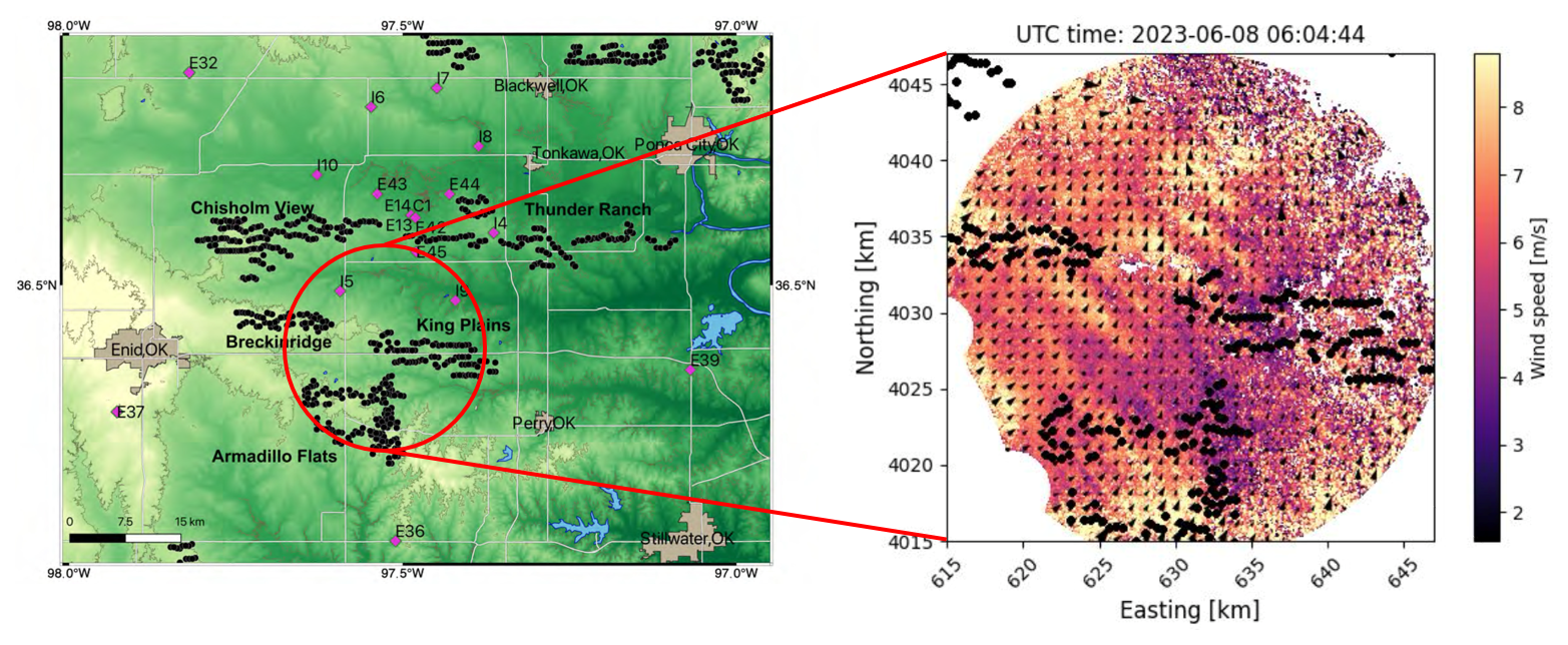
Figure 1 Left: map of AWAKEN measurement sites. The contour value is elevation over the sea level. The terrain is a fluviatile plain with a gradual west-to-east slope (Debnath et al., 2022). This figure is adapted from Moriarty et al. (2024). Right: radar measurement taken at approximately the hub height during the AGW event on 8 June 2023. The figure is provided by the US National Renewable Energy Laboratory (NREL). Solid black circles represent wind turbines.

For this study, we focus on the AGW event on 8 June 2023 because its vertical extent spans the rotor layer of a wind turbine. The right panel of Fig. 1 shows the radar observations of this AGW event. The wind speed peaks and troughs elongated in the northwest–southeast direction indicate large-scale wave-like structures flowing over multiple wind farms. These wave-like structures horizontally propagate from southwest to northeast with a wavelength of approximately 2.5 km.

In Fig. 2, the top-left panel shows lidar measurements of wind speed at site A1 during the selected AGW event. The horizontal axis represents a UTC time zone (local time + 5 h), while the vertical axis represents height above ground level. The duration of the AGW event is approximately 1200 s, and the wind speed exhibits low-frequency oscillations with a period of roughly 600 s. The missing observations near the ground will be filled using a natural-neighbor interpolation technique (Allaerts et al., 2023) in the following data assimilation.

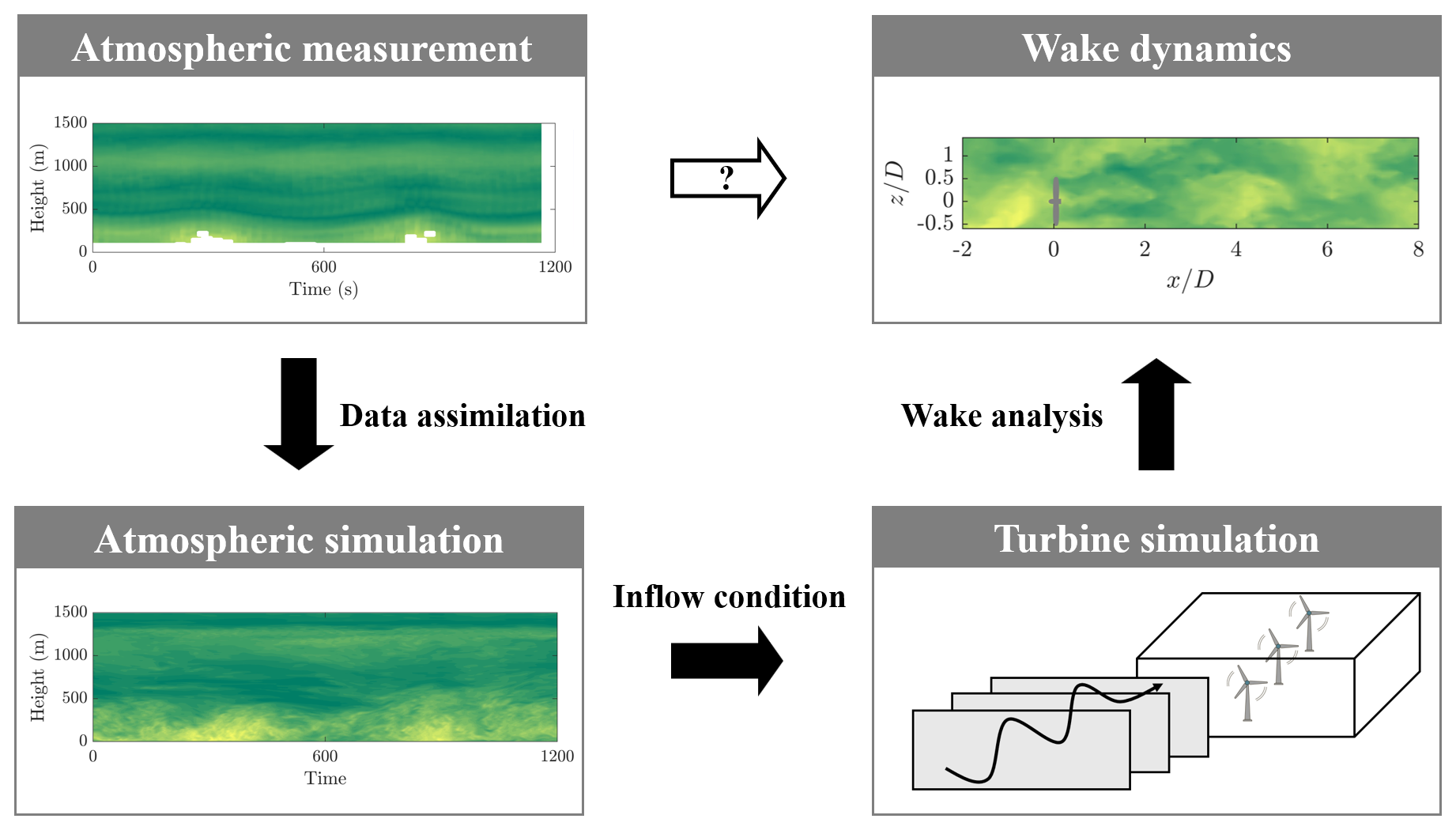
Figure 2 Flow chart of the present measurement-driven LES study. From green to yellow indicates wind speed from 0 to 8 m s⁻¹.

2.2 Measurement-driven LES

A measurement-driven large-eddy simulation (LES) model is developed to simulate turbine flow under AGW inflow conditions. This approach leverages the mesoscale–microscale coupling capability of SOWFA (Simulator for Wind Farm Applications) (Churchfield et al., 2012) and the high-spatio-temporal resolution measurements from the AWAKEN campaign. The simulation is carried out in two stages: (i) inflow simulation, which assimilates AGW measurements into the atmospheric simulation, and (ii) turbine simulation, which generates wind turbine wake flow under the measurement-assimilated inflow condition.

In the first stage, the inflow simulation solves the spatially filtered incompressible Navier–Stokes equations of mass and momentum and the transportation equation of potential temperature. The momentum equation includes two source terms. One source term accounts for mesoscale forcing computed through an indirect profile assimilation method (Allaerts et al., 2020). This method ensures that the LES solution reproduces the time–height wind speed profile shown in the top panel of the bottom-left contour in Fig. 2, thus capturing the key characteristics of the AGW inflow. The other source term in the momentum equation accounts for the Coriolis force induced by planetary rotation.

The potential temperature remains constant below the capping inversion layer and increases linearly in the above regions, which follows the potential temperature profile in conventionally neutral boundary layers. Such a simplification of the thermal stability condition is necessary due to a lack of temperature measurement data. Consequently, the atmospheric condition in our simulation is neutral, whereas, in reality, it could have been either neutral or thermally stable. The inversion layer height is set as 1250 m based on the vertical distribution of wind speed shown in the left column of Fig. 2. Subgrid-scale effects are modeled using a standard turbulent kinetic energy (TKE) equation (Deardorff, 1980).

The computational domain is configured as a straight channel with dimensions of $\mathrm{3000}\times \mathrm{3000}\times \mathrm{1500}$ m in the streamwise, spanwise, and vertical directions, respectively. The domain is discretized into $\mathrm{300}\times \mathrm{300}\times \mathrm{150}$ grid cells. A slip wall condition is applied at the upper boundary, with velocity gradients set to zero, while the bottom boundary uses a local-similarity-based logarithmic wall model (Moeng, 1984) to account for viscous and subgrid-scale stresses. The effective roughness height is set to 0.1 m, representing typical onshore terrain. Periodic conditions are applied at the lateral boundaries.

The inflow simulation runs for 2400 s, with the first 1200 s allocated for spin-up and the remaining 1200 s representing the AGW event. The LES solution for velocity and temperature at the upstream boundary is saved at a time step of 0.5 s during the last 1200 s, providing inflow conditions for the subsequent turbine simulation. For comparison, we also simulate a standard atmospheric boundary layer (non-AGW) as an inflow condition.

The left panel of Fig. 2 shows time–height histories from simulations (bottom) and measurements (top) for the AGW case. The simulation not only captures the low-frequency wind speed oscillations but also resolves turbulence structures with a higher spatio-temporal resolution. To further quantify this comparison, we show wind profiles in Fig. 3 and wind speed time series in Fig. 4. In Fig. 3, the profiles of AGW crest (panel a), AGW trough (panel b), and mean (panel c) wind speed from the simulation follow those from the measurements. The turbulent kinetic energy (panel d) from the simulation increases at lower heights, similarly to the trend in the measurement but with higher magnitudes. Such a difference is expected because the simulation resolves more turbulence motions. This explanation is supported by the wind speed time series in Fig. 4, which indicates that the simulation captures smaller-scale turbulent fluctuations in addition to large-scale AGW oscillations observed from the measurements.

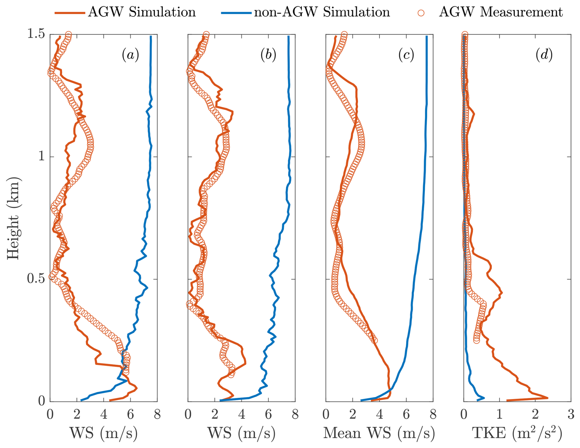
Figure 3 Vertical profiles of (a) instantaneous wind speed at AGW crest, (b) instantaneous wind speed at AGW trough, (c) mean wind speed, and (d) turbulent kinetic energy. Data are compared between the AGW simulation (red lines), non-AGW simulation (blue lines), and AGW measurement (red circles). The mean wind speed and turbulent kinetic energy at lower heights are not shown for the AGW measurement due to the lack of wind speed data over several time steps, as shown in the top-left contour in Fig. 2.

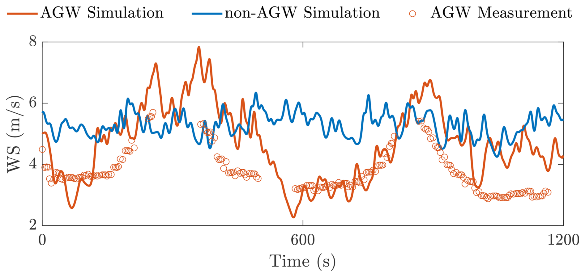
Figure 4 Time series of wind speed at hub height. Data are compared between the AGW simulation (red lines), non-AGW simulation (blue lines), and AGW measurement (red circles).

Figures 3 and 4 also show comparisons between the AGW (red lines) and non-AGW (blue lines) simulations. For the AGW case, both the instantaneous (see Fig. 3a and b) and mean (see Fig. 3c) wind speed profiles exhibit a high-speed zone at lower heights, indicating the presence of low-level jets. Such vertical profiling differs significantly from the non-AGW one, where mean wind speed typically increases monotonically with height above the ground (see Fig. 3c). Besides, the AGW case shows higher turbulence kinetic energy at lower heights (see Fig. 3d), which is also evident in the larger wind speed fluctuation magnitudes shown in Fig. 4.

In the second stage, the turbine simulation incorporates the effect of wind turbines as additional source terms in the Navier–Stokes momentum equations. The turbine is modeled using the NREL 5 MW reference turbine (Jonkman, 2009), a three-bladed horizontal-axis turbine with a rotor diameter of D=126 m and a hub height of 90 m. This open-source turbine model is used as a proxy for the 2.8 MW General Electric turbines deployed at the King Plains wind farm. Regarding the geometric features, the differences between the GE 2.8 MW turbine and the NREL 5 MW reference turbine are minor: rotor diameter of 127 m vs. 126 m and hub height of 88.5 m vs. 90 m, respectively. The turbine cut-in wind speed is 3 m s⁻¹.

The turbine is placed 5 D downstream of the inflow boundary, and its forcing is modeled using an actuator disk method with rotation (Wu and Porté-Agel, 2011). While the effects of the nacelle and tower are neglected, this method has been demonstrated to show good agreement with wind tunnel measurements and high-fidelity numerical simulations in the far-wake region (Wu and Porté-Agel, 2011; Stevens et al., 2018), which primarily influences wind farm flow characteristics. The turbine operates at a constant rotational speed of nine rotations per minute (9 RPM). This simplified operating condition is used because the present work serves as a preliminary investigation of a single turbine rather than as a detailed simulation of the exact AWAKEN wind farm.

The inflow simulation slices are imposed at the inflow boundary. A Rayleigh damping layer is applied at the outflow boundary to prevent unphysical wave reflections. The remaining boundary conditions (top, bottom, and lateral) are consistent with those used in the precursor inflow simulation. After convergence, the flow field and turbine power are saved. The flow data collection subdomain spans $-\mathrm{2}\le x/D\le \mathrm{8}$, $-\mathrm{2}\le y/D\le \mathrm{2}$, and $-\mathrm{0.7}\le z/D\le \mathrm{2}$, where x, y, and z represent the streamwise, spanwise, and vertical coordinates, respectively. The origin is located at the turbine hub center.

The turbine simulation provides wake flow data which can be used to analyze the wake dynamics under the AGW inflow condition, referred to as the AGW case. For comparison, we also perform a turbine simulation without AGWs, referred to as the non-AGW case. In this case, a conventionally neutral boundary layer is simulated as the inflow condition using a wall-modeled LES method designed to capture scaling laws for both mean velocity and velocity fluctuations (Feng et al., 2024b). Once the inflow simulation reaches a statistically steady state, the flow data are collected for an additional 1200 s, as in the AGW case. Both the mean wind speed at the hub height, U_hub=5 m s⁻¹ (consistent with the mean lidar measurements), and the vertical temperature profile remain identical for the AGW and non-AGW inflow conditions.

Throughout this paper, the instantaneous streamwise, spanwise, and vertical velocity components are denoted as u, v, and w, with their time-averaged counterparts denoted as U, V, and W. Time averaging is performed over the 1200 s duration of the AGW event, which corresponds to approximately two wave cycles.

3 Results and discussion

3.1 Wake meandering

Wake meandering refers to large-scale oscillations of the wake flow driven by low-frequency spanwise and vertical velocity fluctuations in the atmospheric flow (Ainslie, 1988). These velocity fluctuations intermittently change the wind direction, causing the wake flow to deflect as if it were a passive tracer. Figure 5 presents instantaneous velocity contours in the spanwise (top) and vertical (bottom) planes for both the AGW (left) and non-AGW (right) cases. The snapshot corresponds to the first peak in wind speed during the AGW event. In both planes, the AGW case causes larger-scale deflections of the wake center, indicative of stronger wake meandering, compared to the non-AGW case. As a result, the AGW case shows a greater range of wake excursions. Specifically, as shown in the left column of Fig. 5, both spanwise and vertical wake excursions extend beyond one rotor diameter for the AGW case, whereas, for the non-AGW case, they only slightly exceed 0.5 times the turbine diameter.

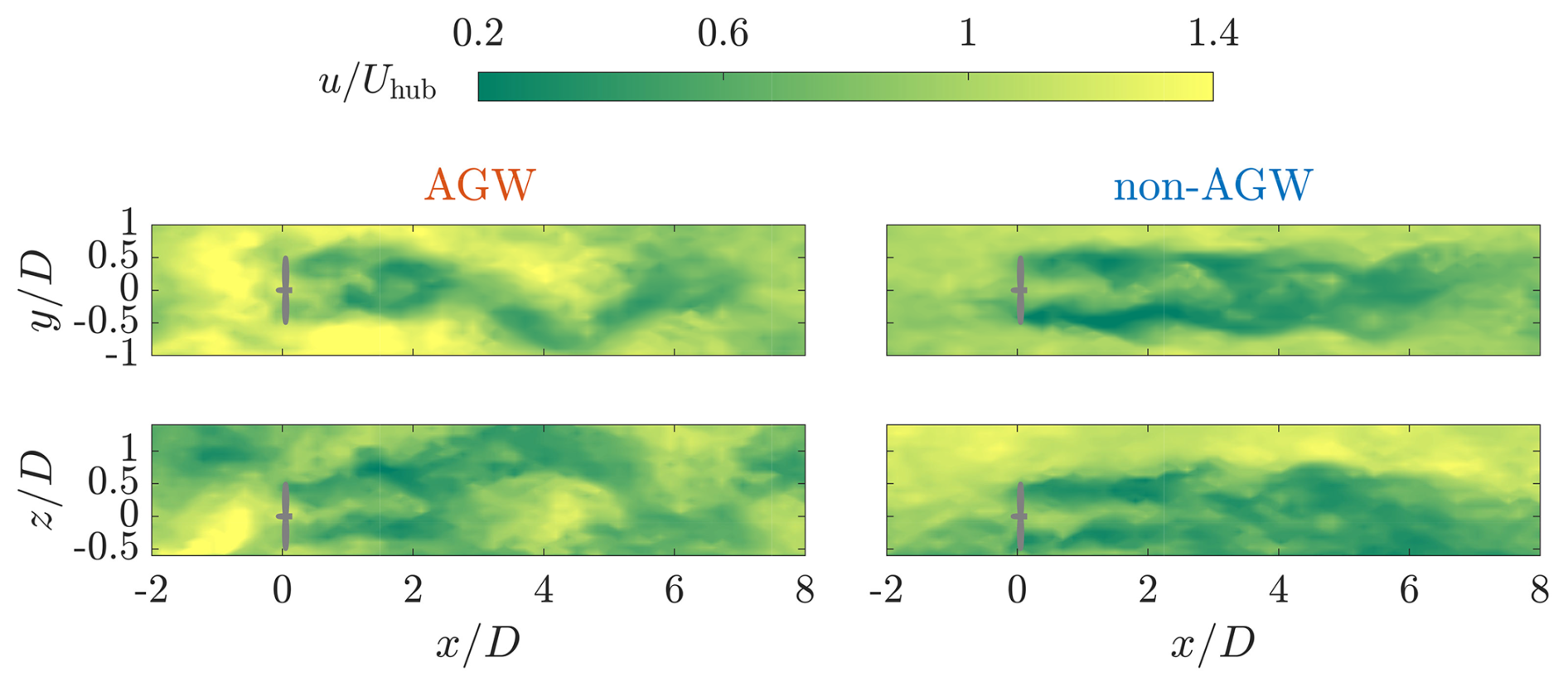
Figure 5 Instantaneous streamwise velocity normalized by U_hub in the spanwise (top) and (bottom) vertical planes passing through the turbine center. The data are compared between the AGW (left) and non-AGW (right) cases. The gray bar in each plot indicates the turbine location.

To quantify the mean amplitude of wake meandering, we use a metric, A_m, defined as the standard deviation of large-scale wake center deflections. The wake centers are determined by first filtering the instantaneous wake deficit flow field with a spatial filter spanning three rotor diameters to isolate meandering motions. The filtered wake deficit is then fitted to a two-dimensional Gaussian profile at each downstream location, following the method described by Trujillo et al. (2011). The location of the maximum wake deficit is taken as the wake center. In both spanwise and vertical directions, the magnitudes of wake center deflections are found to be larger for the AGW case, as evident in Fig. 5. Figure 6 shows A_m in the far-wake region ($\mathrm{4}\le x/D\le \mathrm{8}$). The meandering amplitude generally increases with downstream distance as the wake-center deflection at each downstream location is a cumulative effect of upstream deflections. In both the spanwise and vertical planes, the AGW case results in an A_m value that is nearly double that of the non-AGW case, consistently with the observations in Fig. 5.

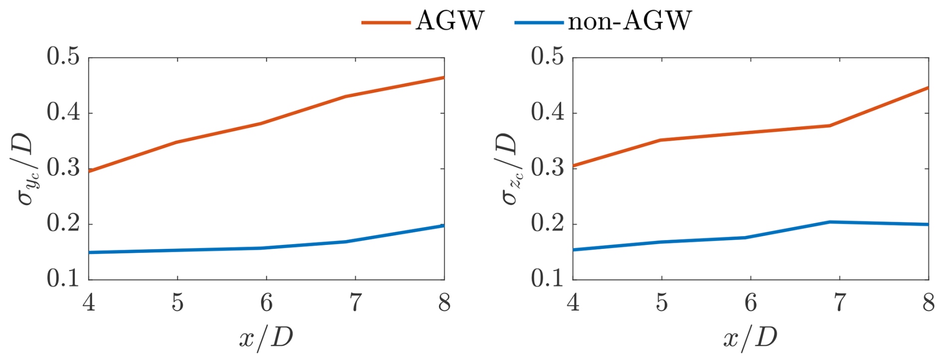
Figure 6 Mean magnitudes of wake meandering in the spanwise (left) and (right) vertical directions for distances of 4 D–8 D downstream of the turbine. The data are compared between the AGW (red line) and non-AGW (blue line) cases.

The stronger wake meandering observed in the AGW case can be attributed to the higher TKE at relatively low frequencies, as will be discussed below in relation to Fig. 9. Previous studies have shown that spanwise and vertical velocity fluctuations in such a frequency range directly drive wake meandering (Larsen et al., 2008; Feng et al., 2022, 2024a). This finding is consistent with the work of Wise et al. (2025), which reported that AGWs can increase overall turbulence levels and amplify horizontal wake meandering.

3.2 Wake turbulence generation

While wake meandering is driven by large-scale velocity fluctuations, wake turbulence is predominantly generated through convective instabilities associated with smaller-scale velocity fluctuations (Heisel et al., 2018; Feng et al., 2022). The convective instability mechanism suggests that TKE generation in the wake arises from the selective amplification of upstream velocity fluctuations by shear instabilities induced by wake shear (Heisel et al., 2018; Foti et al., 2018; Feng et al., 2024c; Li and Yang, 2024). The streamwise, spanwise, and vertical velocity fluctuations are $u^{\prime }=u-U$, $v^{\prime }=v-V$, and $w^{\prime }=w-W$, respectively. TKE is then calculated as $\stackrel{\mathrm{‾}}{{u^{\prime }}^{\mathrm{2}}}+\stackrel{\mathrm{‾}}{{v^{\prime }}^{\mathrm{2}}}+\stackrel{\mathrm{‾}}{{w^{\prime }}^{\mathrm{2}}}$, where the overlines indicate time averaging.

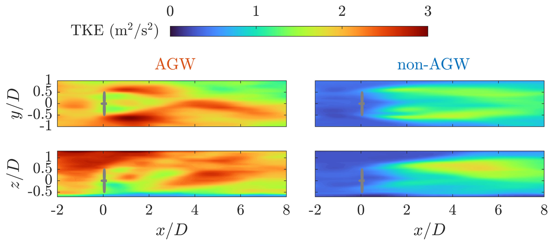
Figure 7 TKE in the spanwise (top) and vertical (bottom) planes passing through the turbine center. The data are compared between AGW (left) and non-AGW (right) cases.

Figure 7 shows the TKE in the spanwise (top) and vertical (bottom) planes for the AGW (left) and non-AGW (right) cases. Compared to the non-AGW case, the AGW case exhibits higher TKE levels in both the inflow and wake regions but lower TKE generated in the wake region when normalized by the inflow TKE. Herein, we define a measure for such inflow-normalized TKE generation as $\mathrm{\Delta }{\mathrm{TKE}}^{*}=(\mathrm{TKE}-{\mathrm{TKE}}_{\mathrm{in}})/{\mathrm{TKE}}_{\mathrm{in}}$, where TKE_in, where TKE_in is the TKE at $x/D=-\mathrm{2}$. The TKE field is spatially averaged over the rotor disk area at each streamwise location.

The left panel in Fig. 8 shows streamwise variation of ΔTKE^* for the AGW and non-AGW cases. For the AGW case, ΔTKE^* initially remains close to zero before decreasing slightly in the far-wake region. By contrast, in the non-AGW case, ΔTKE^* increases sharply to approximately 2 and maintains similar values in the far-wake region, indicating that the wake TKE is nearly 3 times the inflow TKE. The significantly lower ΔTKE^* in the AGW case can be attributed to reduced wake shear, which results from faster wake recovery, as we will discuss in Sect. 3.3.

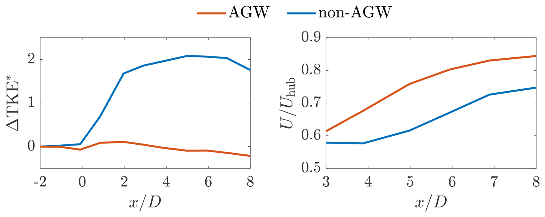
Figure 8 Left: inflow-normalized TKE generation, $\mathrm{\Delta }{\mathrm{TKE}}_{\mathrm{mean}}^{*}$, at each streamwise location. Right: mean streamwise wake deficit along the turbine centerline. The data are compared between the AGW (red line) and non-AGW (blue line) cases.

To investigate the time-varying characteristics of wake turbulence generation, we applied Fourier transforms to the time series of velocity fluctuations to compute the power spectral density of TKE, ${\mathit{\varphi }}_{\mathrm{TKE}}={\mathit{\varphi }}_u+{\mathit{\varphi }}_v+{\mathit{\varphi }}_w$ (where ϕ_u, ϕ_v, and ϕ_w represent the power spectral density of u^′, v^′, and w^′, respectively). Figure 9 shows TKE spectra multiplied by frequency, fϕ_TKE, at various Strouhal numbers, $St=fD/U_{\mathrm{hub}}$ (f is the frequency, D is the rotor diameter, and U_hub is the hub height mean inflow wind speed). Note that the inverse of the Strouhal number corresponds to the wavelength normalized by the rotor diameter, indicating the characteristic turbulence length scales. The area under the spectral curve corresponds to the TKE within a specific frequency range. The spectra are compared between the AGW (top) and non-AGW (bottom) cases for both inflow and wake regions and between the downstream 4 D (left) and 8 D (right) cases for the wake region.

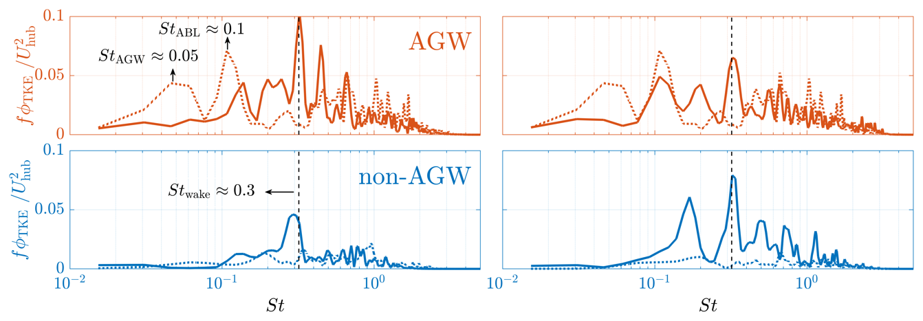
Figure 9 TKE spectra multiplied by the frequency f and non-dimensionalized by $U_{\mathrm{hub}}^{\mathrm{2}}$ as a function of Strouhal number $\mathit{St}=fD/U_{\mathrm{hub}}$. The data are compared between the AGW (top) and non-AGW (bottom) cases. The dotted and solid lines represent spectra calculated for the inflow ($(x/D,y/D,z/D)=(-\mathrm{2},\mathrm{0},\mathrm{0})$) and wake, respectively. The wake spectra in the left and right panels are 4 D and 8 D downstream, respectively.

The inflow spectrum for the AGW case reveals two distinct peaks: (i) a lower-frequency peak at St_AGW≈0.05, corresponding to the AGW wavelength of approximately 2.5 km, highlighting the capability of the precursor inflow simulation to capture the AGW event, and (ii) a higher-frequency peak at St_ABL≈0.1, associated with the atmospheric boundary layer thickness of approximately 1250 m, as indicated by the inversion capping layer height in the top-left contour of Fig. 2. For wall-bounded flows at high Reynolds numbers (e.g., atmospheric boundary layers), Smits et al. (2011) reported that the pre-multiplied TKE spectra in the logarithmic and outer regions exhibit a large-wavelength/low-frequency peak associated with the boundary layer thickness (i.e., the inversion layer height in the atmospheric boundary layer). This peak arises from the presence of large-scale, streamwise-elongated structures with characteristic length scales in the order of the boundary layer thickness (Hutchins et al., 2012).

Despite differences in the peak frequencies of inflow TKE, the wake TKE for both AGW and non-AGW cases is concentrated within a similar frequency range, $\mathrm{0.1}<\mathit{St}<\mathrm{1}$, with a peak at St_wake≈0.3. This frequency peak, which is independent of turbine design and operating conditions, serves as an indicator of convective shear instabilities in far-wake dynamics (Foti et al., 2018; Heisel et al., 2018). Therefore, we conclude that the presence of AGWs does not alter the dominant mechanism of wake turbulence generation. For both the AGW and non-AGW cases, such a frequency peak becomes less prominent in 8 D downstream, as seen in Fig. 9, because wake recovery has largely weakened shear instabilities in this region.

While the mechanism of turbulence generation remains consistent, the AGW and non-AGW cases exhibit differences in their spectral characteristics. For the AGW case, the inflow low-frequency peaks are suppressed by the wake flow and re-energized further downstream. For example, St_ABL is re-established in the wake spectra for the 8 D case. Additionally, there is a notable peak between St_ABL and St_Wake in the wake spectra. The origin of this peak is currently unclear. By comparison, for the non-AGW case, the inflow TKE magnitudes are significantly amplified in the wake TKE spectra. This provides spectral evidence supporting the observation in Fig. 7, which shows that fractional TKE generation is higher in the non-AGW case.

3.3 Mean wake recovery

The expansion of the mean wake flow is driven by a combined effect of wake meandering and turbulent mixing in the instantaneous wake flow. Consequently, larger meandering amplitudes can lead to greater wake expansion and faster recovery. In this section, we analyze the characteristics of the mean wake flow to support the findings in Sect. 3.1, which suggest that AGWs enhance wake meandering.

Figure 10 shows time-averaged streamwise velocity contours in the spanwise (top) and vertical (bottom) planes for the AGW (left) and non-AGW (right) cases. The velocity magnitudes are normalized by U_hub. For all plots, the wake region ($\mathrm{0}\le x/D\le \mathrm{8}$) exhibits a velocity deficit compared to the inflow region ($-\mathrm{2}\le x/D\le \mathrm{0}$), as might be expected. However, in both the spanwise and vertical directions, the wake velocity recovers more quickly towards the ambient velocity for the AGW case. Additionally, as shown in the bottom row of Fig. 10, the AGW and non-AGW cases exhibit distinctly different vertical profiles in the inflow region. While the non-AGW inflow follows a standard boundary layer profile, the AGW inflow shows a low-level jet with the jet nose located near hub height. These low-level jets are also evident in the time–height wind speed history depicted in the left column of Fig. 2.

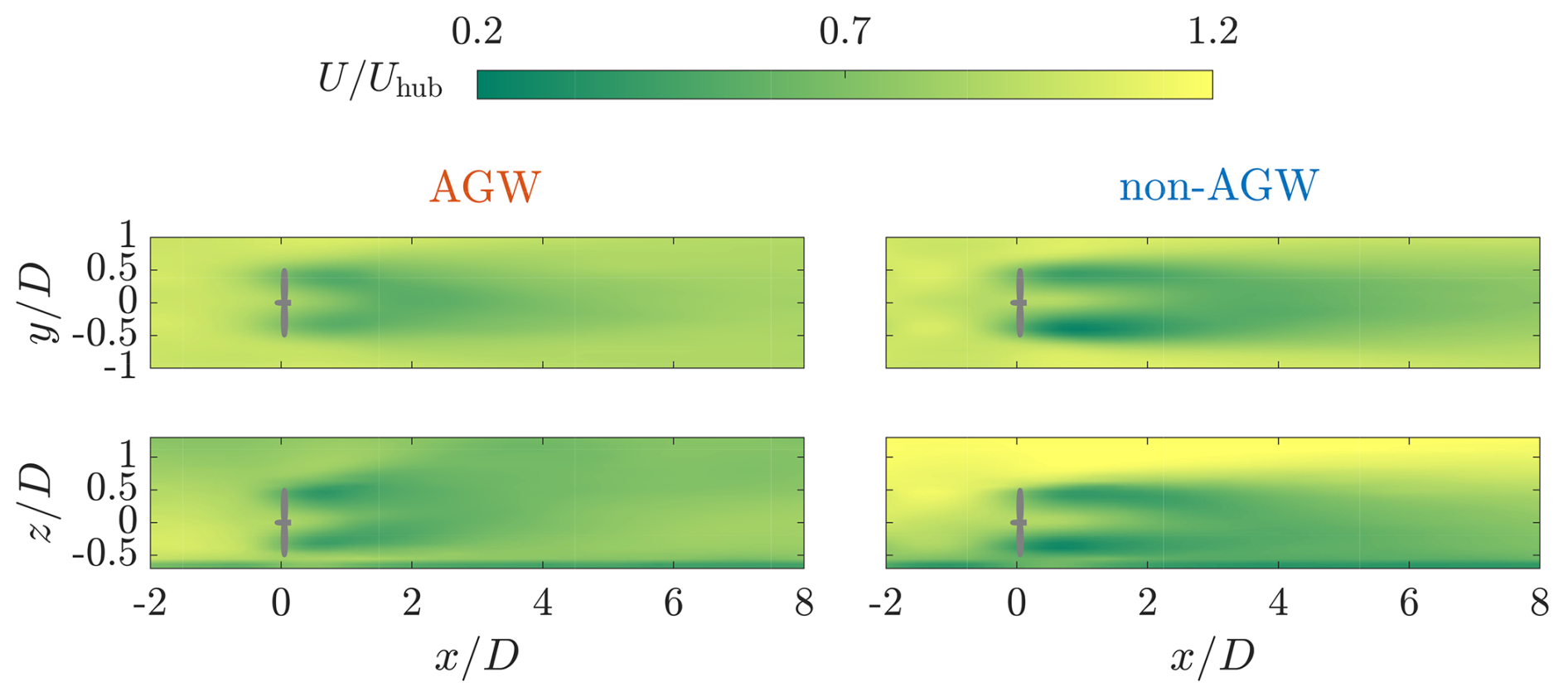
Figure 10 Mean streamwise velocity normalized by U_hub in the spanwise (top) and vertical (bottom) planes passing through the turbine center. The data are compared between AGW (left) and non-AGW (right) cases. The gray bar in each plot indicates the turbine location.

In order to provide a quantitative comparison, the right panel in Fig. 8 shows the U_hub-normalized mean streamwise velocity along the turbine centerline in the wake region. In both the AGW and non-AGW cases, the velocity initially decreases as a result of the pressure recovery immediately behind the rotor and due to the speed-up region near the turbine center gradually diffusing due to momentum exchange. The velocity then begins to recover from approximately $x/D=\mathrm{3}$, where the wake deficit becomes Gaussian-shaped. At $x/D=\mathrm{8}$, the velocity recovers to approximately 90 % of the ambient velocity for the AGW case compared to around 75 % for the non-AGW case.

The faster mean wake recovery in the AGW case can be attributed to two key factors: (i) stronger wake meandering, with the inflow spectra in Fig. 9 showing that the AGW inflow contains more intense large-scale turbulent structures, leading to greater meandering amplitudes and, consequently, larger mean wake expansion (Ainslie, 1988; Larsen et al., 2008), and (ii) higher turbulence levels, with the mean turbulent kinetic energy contours in Fig. 7 shoing significantly higher turbulence levels in the AGW case. The increase in TKE enhances turbulent mixing, making the velocity recovery faster in the wake region.

3.4 Power output of waked turbines

In this section, we analyze the power output of turbines operating in wake regions to validate the dominant role of convective instabilities in wake turbulence generation, as discussed in Sect. 3.2. We simulated two turbines – T1 and T2 – arranged in a streamwise column under AGW inflow conditions, as shown in Fig. 11. Two turbine spacing cases are set: 4 D and 8 D spacings, corresponding to the downstream 4 D and 8 D wake spectra in Fig. 9.

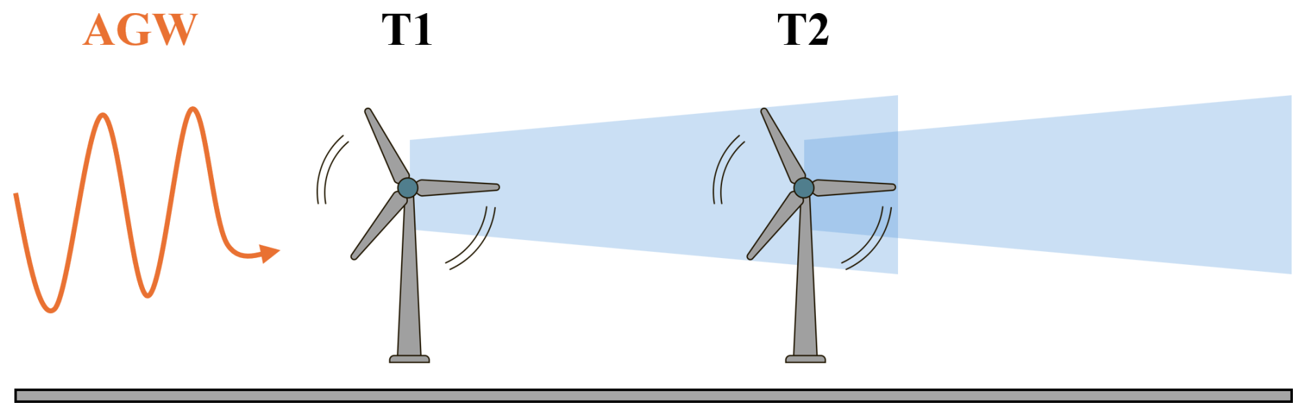
Figure 11 Schematic of the simulation of two turbines under the AGW inflow condition. From upstream to the downstream is subsequently T1 and T2.

Figure 12 shows the time series (left) and spectra (right) of turbine power for T1 and T2 with 4 D (top) and 8 D (bottom) spacings. For the 4 D spacing case, the presence of AGWs induces large-scale power oscillations at the first turbine (T1), which are strongly attenuated at the downstream turbines (T2). For the 8 D spacing case, the attenuation of power oscillations is weaker, and T2 still exhibits visible peaks with a time delay relative to T1. The difference in power attenuation between 4 D and 8 D spacing is also evident in the corresponding spectra. This behavior is because, as we showed in Fig. 9, the shear instability mechanism that damps low-frequency velocity fluctuations becomes weaker further downstream.

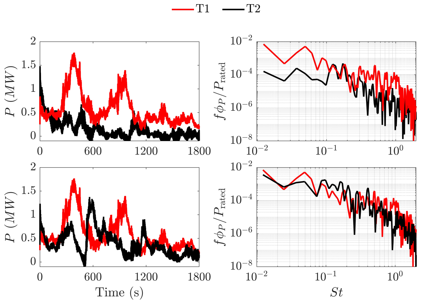
Figure 12 Time series (left) and spectra (right) of turbine power for the two-turbine simulations with 4 D (top) and 8 D (bottom) spacings during the AGW event.

For both 4 D and 8 D spacing, T2 exhibits low-frequency power peaks, although with lower magnitudes and a time delay of approximately 100 s compared to T1. Considering the advection velocity of the AGWs (U_hub=5 m s⁻¹) and the turbine spacing, these peaks could be caused by the AGW event: T2 occasionally operates in large-scale AGW flow structures when the wake behind T1 meanders away, temporarily exposing T2 to the undisturbed AGW inflow. Additionally, there are occasions of negative power. This is because we set in the simulation a constant rotational speed of 9 RPM. At low wind speeds, the aerodynamic torque is not enough to overcome generator and drivetrain losses. As a result, the reported power output can be negative, meaning the turbine is consuming electrical power to keep the generator running.

4 Conclusions

By simulating turbine flow under an AGW event and a standard atmospheric boundary layer (non-AGW), we investigate the impact of AGWs on two key phenomena in wind turbine wake dynamics: wake meandering and wake turbulence generation. Additionally, we analyze mean wake recovery and turbine power fluctuations to support our findings.

Firstly, AGWs result in stronger low-frequency, meandering motions in the wake region. This is attributed to two factors: (i) large-scale AGW flow structures generate low-frequency, large-magnitude velocity fluctuations in both the spanwise and vertical directions, amplifying wake meandering, and (ii) smaller-scale turbulent structures (with length scales greater than three rotor diameters) become more intense due to the elevated turbulence levels. The combination of stronger wake meandering and enhanced turbulent mixing in the instantaneous wake flow leads to faster mean wake recovery under AGW inflow conditions.

Secondly, TKE spectra in the wake region consistently peak at a Strouhal number of approximately 0.3 for both AGW and non-AGW cases, even though the dominant frequencies in the AGW inflow are significantly lower. This finding suggests that turbulence generation in the far-wake region adheres to the convective instability mechanism in both cases. Compared to the non-AGW case, the AGW case exhibits higher inflow TKE levels but a lower amplification factor via convective instabilities in the wake region, likely due to reduced wake shear resulting from faster wake recovery. To further support this conclusion, we examine the power production of two turbines arranged in a streamwise column under AGW inflow conditions. Large-scale AGW flow structures induce significant low-frequency power fluctuations at the most upstream turbine. However, these fluctuations are significantly attenuated at the two downstream turbines, which predominantly operate within the wake regions. This observation underscores the dominant role of convective instabilities in wake turbulence generation.

These findings offer insights for wake modeling under realistic atmospheric conditions, particularly in the presence of transient phenomena such as AGWs. Furthermore, the current measurement-driven LES method can serve as a robust tool for understanding and modeling the inter-scale coupling between mesoscale synoptic forcing and microscale wind farm flow dynamics.

The present work is intended as a case study focusing on a specific AGW event. Future studies should incorporate AGW events originating from various sources and with different wavelengths to comprehensively understand their roles in turbine wake and wind farm flows. Additionally, extending the measurement-driven LES method to other transient atmospheric phenomena, such as convective structures and low-level jets, would be a promising direction for further investigation.