The influence of flow-field representation on electrical power and fatigue-load surrogate modelling in offshore wind farms

High-fidelity aeroelastic simulations provide accurate predictions of electrical power and structural fatigue loads in wind farms but remain computationally expensive for optimisation, control, and digital-twin applications. Machine-learning surrogate models offer an efficient alternative, and recent studies have shown that both surrogate architecture and inflow representation influence predictive performance. However, it remains unclear how the amount and form of retained rotor-plane inflow information affect electrical power and fatigue-load prediction. This study evaluates four input configurations derived from temporally aggregated rotor-plane inflow data from the publicly available HAWC2Farm Lillgrund dataset. A minimal baseline representation retains only the spatial averages of the temporal-mean wind-speed and temporal-variance fields, while a flattened full-grid representation retains all rotor-plane measurements. Principal component analysis (PCA) provides a compact representation of the full input, and a two-dimensional representation preserves the original rotor-plane topology. The baseline, flattened, and PCA configurations are compared using the same SimpleMLP architecture under 5-fold GroupKFold cross-validation, while the two-dimensional spatial representation is evaluated separately using a convolutional neural network as a topology-aware modelling configuration. For electrical power prediction, the two-variable baseline already retained most of the predictive information, achieving an RMSE of approximately 2.2 % of rated power, while the distributed representations further reduced the absolute prediction error. For fatigue-load prediction, the effect of distributed inflow information was substantially more load-channel dependent, with only a marginal difference for tower-base fore–aft bending but much larger differences for blade-root edgewise and main-bearing bending. Within the fixed-architecture comparison, the PCA representation achieved the highest accuracy for electrical power prediction while reducing the input dimensionality from 1800 variables to 128 principal components. In contrast, the topology-aware CNN achieved the lowest prediction errors across all 12 fatigue-load components. These results show that the value of distributed rotor-plane information differs between the two prediction tasks and that the most effective representation–architecture configuration among those evaluated depends on the prediction objective.

1 Introduction

The increasing size and complexity of modern wind farms have intensified the need for computationally efficient tools capable of accurately predicting electrical power and structural fatigue loads. These quantities are fundamental to wind farm design, control, optimisation, and lifetime assessment, where large numbers of aeroelastic simulations are typically required to evaluate different operating conditions, control strategies, and environmental scenarios. Although high-fidelity aeroelastic tools provide accurate predictions of turbine response, their computational cost makes them impractical for many optimisation, control, and digital twin applications. Consequently, data-driven surrogate models have become an increasingly attractive alternative for approximating electrical power and structural loads at a fraction of the computational cost of conventional aeroelastic simulations (Gasparis et al., 2020; Haghi and Crawford, 2024; Singh et al., 2024).

A wide variety of surrogate modelling approaches have been proposed for wind energy applications. Early studies compared conventional regression techniques, artificial neural networks, and Gaussian process regression for predicting electrical power and fatigue loads under varying operating conditions (Gasparis et al., 2020). More recent work has explored probabilistic surrogate models capable of quantifying prediction uncertainty (Singh et al., 2024) and graph neural networks for jointly predicting local inflow conditions, electrical power, and fatigue loads across arbitrary wind farm layouts (Duthé et al., 2023). Together, these studies demonstrate the growing use of machine learning methods for approximating aeroelastic responses across a range of wind-energy applications.

Several recent studies have investigated how different representations of rotor-plane inflow influence surrogate model performance. Shaler et al. (2022) demonstrated that temporal-mean rotor-plane velocity measurements were sufficient for accurately predicting mean turbine quantities, whereas predicting fatigue loads and other higher-order statistics additionally required information describing the temporal variability in the inflow. Similarly, Liew et al. (2023a) demonstrated that a surrogate model combining proper orthogonal decomposition (POD) of rotor-plane inflow fields with an artificial neural network substantially improved fatigue-load prediction. Guilloré et al. (2024) proposed a surrogate model based on sector-averaged inflow quantities and demonstrated that this simplified representation remained sufficient to accurately predict damage equivalent loads under unwaked, waked, wake-steering, and induction-control operating conditions. More recently, Ramaswamy et al. (2026) compared a hierarchy of local inflow parameterisations ranging from rotor-averaged quantities to POD-based and rotor-resolved representations, showing that rotor-averaged parameterisations exhibited the largest prediction errors, whereas higher-fidelity representations more reliably captured wake-induced loading. Taken together, these studies demonstrate that the representation of rotor-plane inflow can influence surrogate model performance for fatigue-load prediction.

The rotor-plane inflow representation studies above all investigate structural fatigue-load prediction. In contrast, studies that jointly predict electrical power and structural loads have primarily focused on comparing surrogate modelling algorithms while employing a single inflow representation (Gasparis et al., 2020). Consequently, it remains unclear whether the representation that is most appropriate for fatigue-load estimation is also optimal for electrical power prediction when both prediction tasks are based on the same underlying rotor-plane inflow information.

The objective of this work is therefore to investigate how the amount and form of retained rotor-plane inflow information influence surrogate modelling performance for two fundamentally different prediction tasks: electrical power and fatigue-load estimation. Four input configurations are considered: a minimal spatially aggregated baseline, the full flattened rotor-plane field, a principal component representation, and a topology-preserving two-dimensional representation. The baseline, flattened, and principal component configurations are evaluated using the same SimpleMLP architecture to provide a fixed-architecture comparison, while the spatial representation is evaluated separately using a convolutional neural network as a topology-aware modelling configuration. All experiments are conducted on the publicly available HAWC2Farm Lillgrund dataset (Liew et al., 2023b). This framework enables the predictive value of retaining distributed rotor-plane information to be assessed while examining whether the most effective representation–architecture configuration differs between electrical power and fatigue-load prediction.

2 Dataset description

The dataset used in this study is derived from the large-scale HAWC2Farm simulations of the Lillgrund offshore wind farm introduced by Liew et al. (2023a) and is publicly available through the Technical University of Denmark Data Repository (Liew et al., 2023b). The wind farm consists of 48 wind turbines, each with a rated power of 2.3 MW.

The complete dataset comprises 1000 independent 1 h HAWC2Farm simulations generated under varying inflow conditions, of which 800 simulations are publicly available and used in this study. Each simulation is run at 100 Hz and is characterised by randomly generated atmospheric conditions, including wind direction, ambient wind speed (4–20 m s⁻¹), power-law shear exponent (0.1–0.3), and turbulence intensity (2.5 %–10 %). The wind fields immediately upstream of each turbine are recorded once per second on a uniform 30×30 Cartesian grid spanning an area of 1.1D×1.1D, where the rotor diameter is D=92.6 m.

The dataset is organised into six non-overlapping 10 min intervals for each 1 h simulation. For every turbine and interval, the rotor-plane wind field is temporally aggregated over the corresponding 10 min window to obtain two 30×30 profiles: a mean wind-speed field and a standard-deviation field describing the temporal variability in the inflow at each grid location. Each turbine–interval pair constitutes a single observation, resulting in $\mathrm{48}\times \mathrm{6}=\mathrm{288}$ observations per simulation and a total of 230 400 observations across the 800 publicly available simulations considered in this work.

Each observation comprises a single flattened 1800-dimensional input vector describing the temporally aggregated rotor-plane inflow over the corresponding 10 min interval. This representation is formed by concatenating two 900-dimensional vectors containing the mean and standard deviation of the inflow respectively. Since each 900-dimensional vector corresponds to a uniform 30×30 Cartesian sampling of the rotor plane, the original spatial fields can be recovered by reshaping the input into two 30×30 grids corresponding to the mean and standard deviation respectively. The corresponding outputs comprise the electrical power together with 12 fatigue-relevant damage-equivalent load (DEL) quantities evaluated over the same turbine and 10 min interval. The predicted fatigue load components are summarised in Table 1.

Table 1 Summary of predicted fatigue load components and the physical load directions specified in the released dataset documentation. All quantities are reported as 10 min damage-equivalent loads (DELs) in kNm.

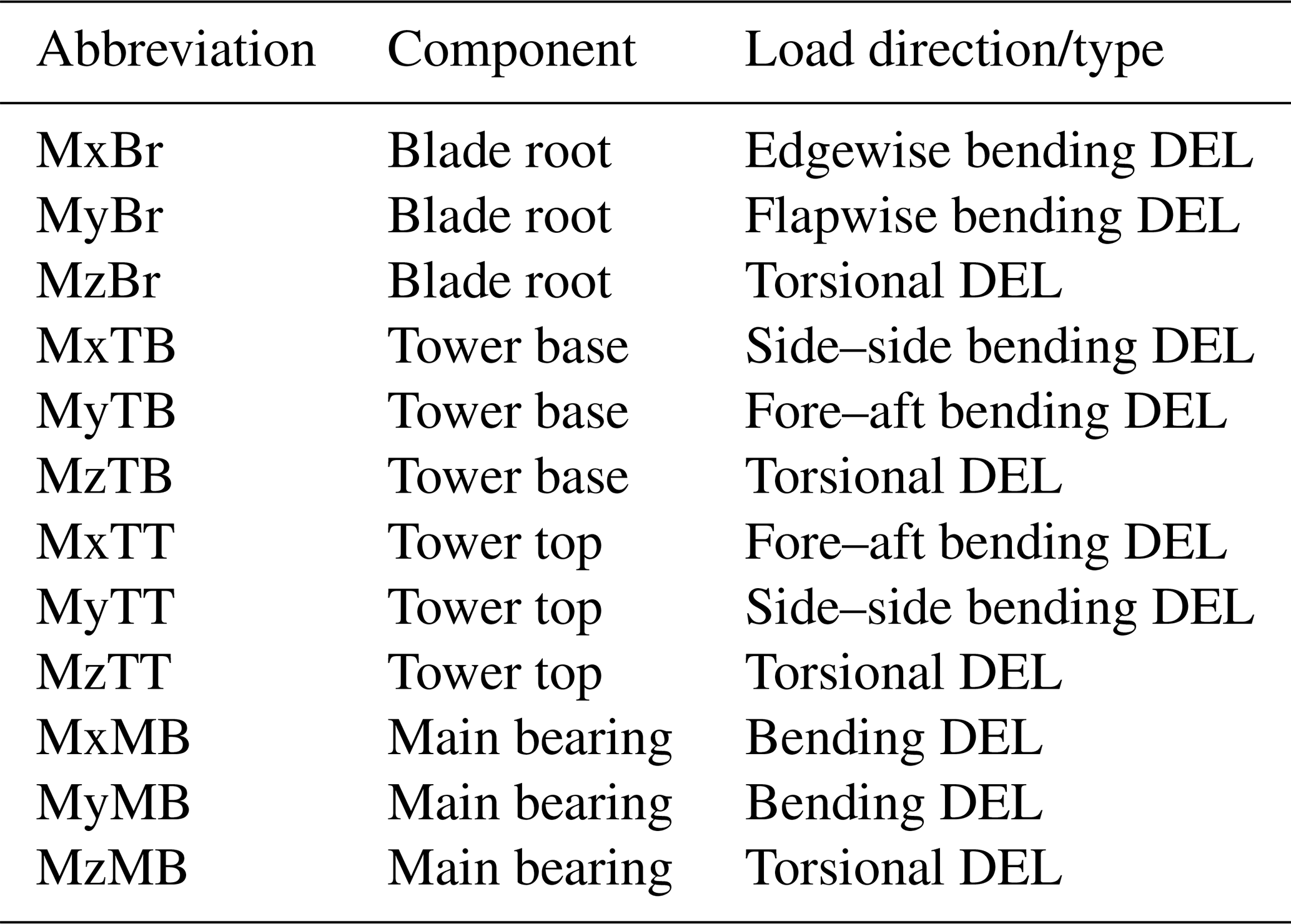
The load-channel abbreviations follow the naming convention used in the released HAWC2Farm dataset. The associated physical load directions are those specified in the dataset documentation. At the blade root, M_x, M_y, and M_z denote edgewise bending, flapwise bending, and torsion respectively. At the tower base, they denote side–side bending, fore–aft bending, and torsion, while at the tower top they denote fore–aft bending, side–side bending, and torsion. For the main bearing, M_x and M_y are reported as bending components and M_z as torsion. The x, y, and z labels should therefore be interpreted as channel-specific HAWC2 output axes rather than as a single common turbine-fixed coordinate convention. HAWC2 permits structural moment outputs to be expressed in user-selected main-body, global, or local beam coordinate systems, whose orientations may differ between structural components. The generation input files specifying the exact output frame for each released channel are not included with the public dataset; therefore, the physical direction labels provided with the dataset are used here without inferring an unreported common coordinate transformation.

Figure 1 shows an example observation from the dataset after reshaping the flattened input vectors into their original 30×30 spatial representation. The left panel shows the temporally averaged rotor-plane inflow velocity over a representative 10 min interval, while the right panel shows the corresponding temporal standard deviation.

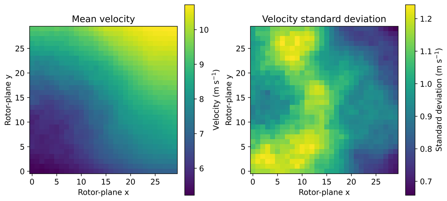
Figure 1 Example rotor-plane wind-field observation reconstructed from the released dataset. The left and right panels respectively show the temporally aggregated mean and standard deviation of the inflow velocity over a representative 10 min interval.

The distribution of the electrical power output is shown in Fig. 2. The observations span the complete operating range of the turbine, from low-power operating conditions to values approaching the rated power of 2.3 MW. This provides a diverse regression target across a wide range of inflow conditions.

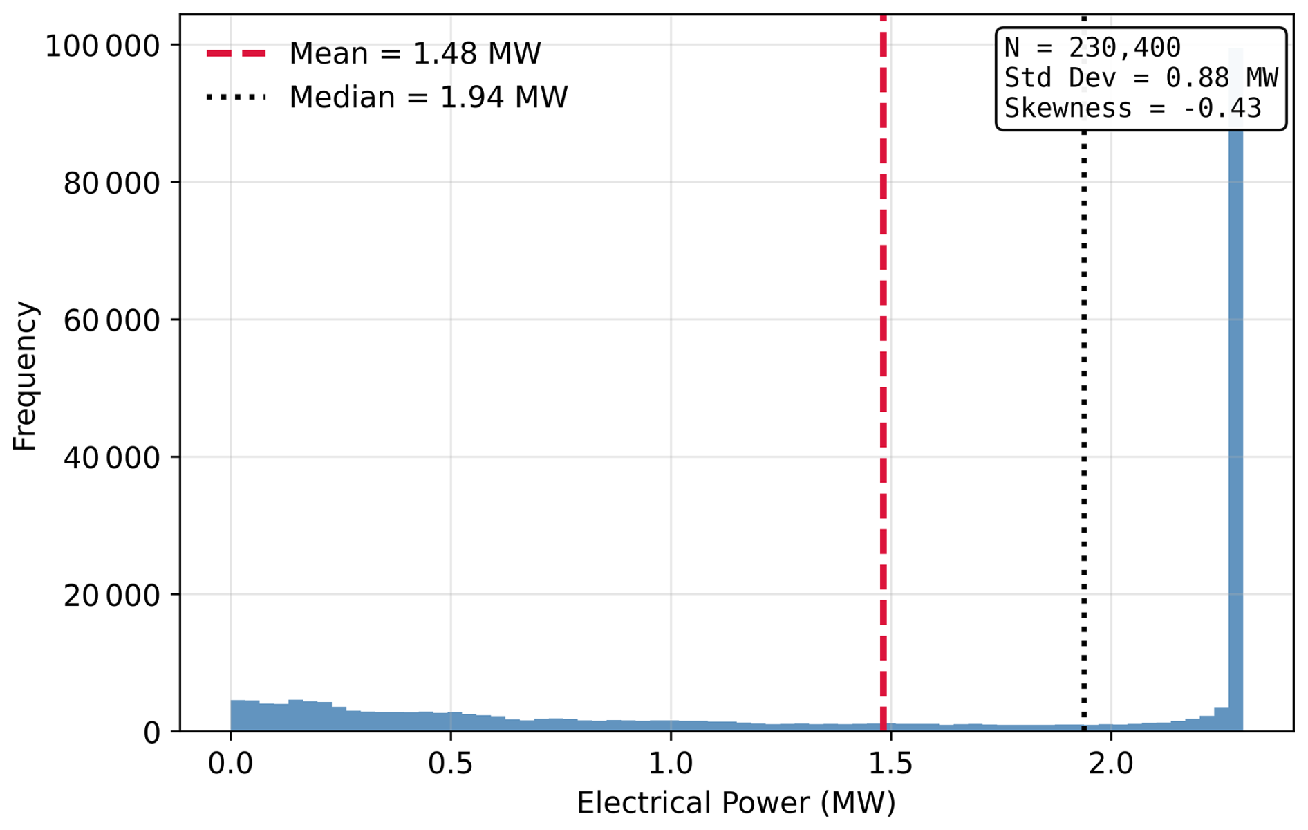
Figure 2 Distribution of electrical power across all observations in the dataset. The dashed red and dotted black lines denote the mean and median electrical power respectively.

Figure 3 summarises the distribution of the 12 fatigue damage-equivalent load (DEL) targets. The different structural components exhibit substantial differences in both their characteristic magnitudes and variability, with load values spanning more than 3 orders of magnitude. A logarithmic vertical axis is therefore used to facilitate comparison across all load components while preserving their physical units.

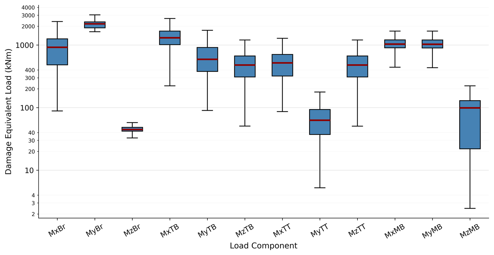
Figure 3 Distribution of the 12 fatigue damage-equivalent load (DEL) targets shown on a logarithmic scale. Boxes represent the interquartile range (IQR), the horizontal red line indicates the median, and whiskers extend to the most extreme observations within 1.5 times the IQR. Outliers beyond the whiskers are omitted for clarity.

3 Input representations

The dataset provides the inflow conditions as two wind-field variables corresponding to the spatial distributions of the mean wind speed and the standard deviation over a 30×30 sampling grid. Although these fields are inherently two-dimensional, the released dataset stores them as two flattened vectors, resulting in an input dimensionality of 1800 features per observation.

This work considers four input configurations derived from the same underlying rotor-plane inflow data. First, a minimal baseline representation is constructed from the spatial averages of the temporal-mean wind-speed and temporal-variance fields, intentionally discarding the distributed rotor-plane information. Second, the released flattened representation is used directly, retaining all 1800 grid-based input variables without explicitly preserving their two-dimensional arrangement. Third, principal component analysis (PCA) is employed to obtain a compact lower-dimensional representation of the full flattened input. Finally, the original spatial structure is restored by reshaping the two wind-field vectors into two 30×30 fields for use with a topology-aware convolutional model.

The baseline, flattened, and PCA configurations are evaluated using the same SimpleMLP architecture to provide a fixed-architecture comparison of input representations. The spatial representation is evaluated separately using a convolutional neural network designed to exploit the two-dimensional topology of the rotor-plane inflow.

3.1 Baseline representation

To provide a minimal-information reference configuration, the rotor-plane inflow was reduced to two spatially aggregated scalar quantities. Let μ_i and σ_i denote the temporal-mean wind speed and temporal standard deviation respectively at grid point i of the 30×30 rotor-plane grid. The baseline mean-wind-speed input is defined as

$$\begin{array}{}\text{(1)}& \overline{\mathit{\mu }}={\displaystyle \frac{\mathrm{1}}{\mathrm{900}}}\sum _{i=\mathrm{1}}^{\mathrm{900}}{\mathit{\mu }}_i,\end{array}$$

while the baseline variance input is defined as

$$\begin{array}{}\text{(2)}& \stackrel{\mathrm{‾}}{{\mathit{\sigma }}^{\mathrm{2}}}={\displaystyle \frac{\mathrm{1}}{\mathrm{900}}}\sum _{i=\mathrm{1}}^{\mathrm{900}}{\mathit{\sigma }}_i^{\mathrm{2}}.\end{array}$$

The released dataset provides the temporal standard-deviation field σ_i at each grid point. Each value is therefore squared first to obtain the corresponding temporal variance ${\mathit{\sigma }}_i^{\mathrm{2}}$, after which the variance field is spatially averaged over the rotor plane. Each observation is consequently represented by the two-dimensional input vector

$$\begin{array}{}\text{(3)}& {\mathit{x}}_{\mathrm{baseline}}=\left[\overline{\mathit{\mu }},\stackrel{\mathrm{‾}}{{\mathit{\sigma }}^{\mathrm{2}}}\right].\end{array}$$

This representation intentionally removes the distributed rotor-plane information retained by the other configurations and provides a minimal-information reference against which the predictive value of spatially distributed inflow information can be assessed.

3.2 Flattened representation

The flattened representation is used directly as provided by the dataset, resulting in an input vector of length 1800 for each observation. No reshaping or dimensionality reduction is applied to the wind field.

Representing the wind field as a one-dimensional feature vector removes the explicit spatial relationships between neighbouring grid locations. Consequently, the representation no longer preserves the geometric arrangement of the wind field, and the learning algorithm receives only an ordered collection of feature values. Any influence of the spatial organisation of the inflow on the prediction of electrical power or fatigue loads must therefore be learned implicitly, rather than being explicitly encoded within the input representation.

Because the input is represented as a feature vector rather than a two-dimensional field, fully connected neural networks provide a natural modelling framework. Unlike convolutional neural networks, which employ local receptive fields and shared kernels to learn hierarchical representations from structured inputs (Lecun et al., 1998), fully connected neural networks learn dense interactions between input features without explicitly encoding spatial locality. The flattened representation therefore provides the full-grid vector configuration used in the fixed-architecture comparison with the baseline and PCA-reduced representations.

3.3 Spatial representation

The spatial representation is obtained by reshaping the two flattened wind-field vectors into two 30×30 grids corresponding to the mean wind speed and the standard deviation. This transformation preserves all original measurements while recovering the original spatial arrangement of the sampling grid. Consequently, each observation is represented as a two-channel tensor with dimensions $\mathrm{2}\times \mathrm{30}\times \mathrm{30}$.

Unlike the flattened representation, the spatial representation explicitly preserves the neighbourhood relationships between adjacent sampling locations. As a result, the geometric organisation of the wind field remains explicitly encoded within the input, making local neighbourhood information directly available to the learning algorithm when predicting electrical power and fatigue loads.

Because the input is represented as a structured two-dimensional field, convolutional neural networks provide a natural modelling framework. Convolutional neural networks apply shared convolutional kernels over local receptive fields to learn hierarchical representations from structured inputs (Lecun et al., 1998). In the present study, the spatial representation is therefore evaluated separately using a CNN as a topology-aware modelling configuration. Its performance is reported as the result of the combined spatial representation and convolutional architecture rather than as an isolated test of representation alone.

3.4 Principal component representation

Principal component analysis (PCA) provides a compact representation of the wind field by projecting the original high-dimensional input onto a lower-dimensional set of orthogonal components ordered according to the amount of variance explained (Jolliffe, 2002; Jolliffe and Cadima, 2016). Unlike the flattened and spatial representations, which preserve all original measurements, the principal component representation expresses the wind field using a reduced set of variables that retain the dominant modes of variation present in the original wind field representation.

By concentrating the majority of the variability into a smaller number of orthogonal components, PCA reduces the redundancy arising from the strong correlations between neighbouring wind-field measurements while retaining the dominant directions of variation in the input data (Jolliffe, 2002). However, because each principal component is formed as a linear combination of all original variables, the explicit spatial arrangement of the sampling grid is no longer preserved.

The principal component representation therefore provides a compact vector-based alternative to the full flattened input. Because both configurations are evaluated using the same SimpleMLP architecture, their comparison allows the effect of dimensionality reduction to be assessed without simultaneously changing the model class.

The subsequent sections introduce the surrogate models and experimental framework used to compare the baseline, flattened, and PCA representations under a fixed fully connected architecture, while evaluating the topology-preserving spatial configuration separately using a convolutional neural network.

4 Experimental setup

4.1 Implementation environment

All experiments were conducted using Python 3.12.10 on a laptop equipped with an Intel(R) Core(TM) i7-14650HX processor (16 cores, 24 logical processors) and 32 GB of RAM. This hardware configuration was sufficient to train all surrogate models on the available dataset without the need for specialised accelerators.

4.2 Training protocol

To obtain robust estimates of predictive performance, all surrogate models were evaluated using 5-fold GroupKFold cross-validation (Hastie et al., 2009). Unlike conventional K-fold cross-validation, GroupKFold partitions the dataset according to predefined groups rather than individual samples. In the present work, each group corresponds to a single simulation realisation, with all 288 turbine–interval observations generated from that simulation assigned exclusively to either the training or validation set within a given fold. This prevents information leakage arising from correlated samples and provides a more realistic assessment of model generalisation to previously unseen inflow conditions.

Within each fold, the input and output normalisation statistics were computed exclusively from the training partition and subsequently applied to both the training and corresponding validation partitions. This ensures that no information from the validation data influenced the preprocessing stage.

The use of GroupKFold also reduces the likelihood that the reported performance results arise from a favourable partitioning of the data. Each surrogate model and input representation was therefore evaluated using the same five data partitions, ensuring that comparisons between configurations are not confounded by differences in the train–validation partitions.

The available dataset 𝒟 of size N is partitioned into K non-overlapping folds $\mathit{\{}{\mathcal{D}}_{\mathrm{1}},{\mathcal{D}}_{\mathrm{2}},\mathrm{\dots },{\mathcal{D}}_K\mathit{\}}$, where each fold contains complete simulation groups. For each fold k, the surrogate model is trained on the union of the remaining K−1 folds and evaluated on the held-out fold 𝒟_k, yielding K independent estimates of predictive performance.

For a generic performance metric M (e.g. RMSE, MAE, or R²), the cross-validated estimate is computed as

$$\begin{array}{}\text{(4)}& \overline{M}={\displaystyle \frac{\mathrm{1}}{K}}\sum _{k=\mathrm{1}}^K{M}_k,\end{array}$$

where M_k denotes the metric evaluated on fold k. The variability in model performance across folds can be quantified using the corresponding standard deviation,

$$\begin{array}{}\text{(5)}& {\mathit{\sigma }}_M=\sqrt{{\displaystyle \frac{\mathrm{1}}{K-\mathrm{1}}}\sum _{k=\mathrm{1}}^K{\left(M_k-\overline{M}\right)}^{\mathrm{2}}}.\end{array}$$

Low variability across folds indicates that surrogate model performance is robust with respect to the particular train–validation partition and is therefore unlikely to result from a favourable split. Throughout this work, the reported performance corresponds to the mean and standard deviation across the five validation folds.

4.3 Evaluation metrics

Surrogate model performance was evaluated using the root-mean-squared error (RMSE), mean absolute error (MAE), and coefficient of determination (R²). RMSE and MAE quantify prediction error in the original physical units of the target variables, while R² measures the proportion of variance in the reference data explained by the surrogate model.

The RMSE is defined as

$$\begin{array}{}\text{(6)}& \mathrm{RMSE}=\sqrt{{\displaystyle \frac{\mathrm{1}}{N}}\sum _{i=\mathrm{1}}^N{\left(y_i-{\widehat{y}}_i\right)}^{\mathrm{2}}},\end{array}$$

where y_i and ${\widehat{y}}_i$ denote the reference and predicted values respectively, and N is the total number of samples.

The MAE is defined as

$$\begin{array}{}\text{(7)}& \mathrm{MAE}={\displaystyle \frac{\mathrm{1}}{N}}\sum _{i=\mathrm{1}}^N\left|y_i-{\widehat{y}}_i\right|,\end{array}$$

which measures the average magnitude of the prediction error without placing greater emphasis on larger deviations.

The coefficient of determination is given by

$$\begin{array}{}\text{(8)}& R^{\mathrm{2}}=\mathrm{1}-{\displaystyle \frac{{\sum }_{i=\mathrm{1}}^N{\left(y_i-{\widehat{y}}_i\right)}^{\mathrm{2}}}{{\sum }_{i=\mathrm{1}}^N{\left(y_i-\overline{y}\right)}^{\mathrm{2}}}},\end{array}$$

where $\overline{y}$ is the mean of the reference values. Values of R² closer to 1 indicate better predictive performance, whereas negative values indicate performance worse than predicting the mean reference value.

For all surrogate models, the reported performance metrics correspond to the mean and standard deviation across the five validation folds.

5 Surrogate models

5.1 Common training configuration

All surrogate models were implemented in Python using the PyTorch deep learning framework (Paszke et al., 2019). Data preprocessing, principal component analysis, and cross-validation were performed using scikit-learn (Pedregosa et al., 2012), with NumPy (Harris et al., 2020) and Pandas (McKinney, 2010) used for numerical computation and data manipulation.

To ensure a fair comparison between surrogate architectures and input representations, all neural networks were trained using a common optimisation strategy. Within each cross-validation fold, the input and output variables were standardised using statistics computed exclusively from the training partition. Specifically, each input and output feature x_j was transformed according to

$$\begin{array}{}\text{(9)}& x_j^{\prime }={\displaystyle \frac{x_j-{\mathit{\mu }}_j}{{\mathit{\sigma }}_j}},\end{array}$$

where x_j denotes the jth input or output feature, and μ_j and σ_j are the corresponding mean and standard deviation computed exclusively from the training partition. The resulting transformations were subsequently applied to both the training and validation data.

Models were trained using mini-batches of 256 samples, while validation employed a batch size of 512. Model parameters were optimised using the AdamW optimiser with an initial learning rate of 10⁻³ and a weight decay coefficient of 10⁻⁴ (Loshchilov and Hutter, 2017). The learning rate was updated after each training epoch using the CosineAnnealingLR scheduler with $T_{max}=\mathrm{50}$ epochs (Loshchilov and Hutter, 2016). The optimisation objective was the mean squared error (MSE) loss, implemented using the MSELoss criterion.

To reduce unnecessary computation and mitigate overfitting, early stopping with a patience of 20 epochs was employed based on the validation loss. Training was performed for a maximum of 200 epochs, with optimisation terminated if the validation loss did not improve for 20 consecutive epochs. The model parameters corresponding to the lowest validation loss were retained for subsequent evaluation.

5.2 Simple multilayer perceptron

The simple multilayer perceptron (SimpleMLP) is used as the common fully connected architecture for the vector-based input representations. As the baseline, flattened, and principal component representations are all expressed as one-dimensional feature vectors, a fully connected network provides a consistent modelling framework without assuming any underlying spatial structure. Using the same architecture across these representations enables their predictive performance to be compared without simultaneously changing the model class.

The network consists of an input layer followed by two fully connected hidden layers containing 256 neurons each, with rectified linear unit (ReLU) activation functions applied after each hidden layer. The resulting network architecture is given by

$$\begin{array}{rl}& \mathrm{Linear}(d_{\mathrm{in}},\mathrm{256})\to \mathrm{ReLU}\\ & \to \mathrm{Linear}(\mathrm{256},\mathrm{256})\to \mathrm{ReLU}\to \mathrm{Linear}(\mathrm{256},d_{\mathrm{out}}),\end{array}$$

where d_in denotes the input dimensionality and d_out the number of prediction targets. For the baseline representation, d_in=2, while for the flattened representation, d_in=1800. For the principal component representation, d_in corresponds to the number of retained principal components determined in the PCA analysis presented subsequently. The output dimensionality is d_out=1 for electrical power prediction and d_out=12 for fatigue-load prediction.

A relatively shallow architecture was deliberately adopted to provide a consistent and computationally efficient modelling framework while avoiding unnecessary model complexity. The use of two hidden layers allows nonlinear relationships between the input features and target variables to be learned while maintaining a relatively simple network architecture. Consequently, differences among the baseline, flattened, and PCA configurations can be interpreted primarily in terms of the input representation rather than differences in architectural complexity.

5.3 Residual multilayer perceptron

The residual multilayer perceptron (ResMLP) extends the SimpleMLP architecture by incorporating residual learning, facilitating the training of deeper fully connected networks while alleviating optimisation difficulties associated with increasing network depth (He et al., 2015; Touvron et al., 2021). Similar to the SimpleMLP, the ResMLP operates directly on one-dimensional feature vectors and is therefore compatible with vector-based input representations.

The network first projects the input feature vector into a 512-dimensional latent feature space through a fully connected layer followed by the SiLU activation function. This latent representation is subsequently processed by a sequence of 12 residual blocks before being mapped to the prediction targets using a final linear output layer. The resulting network architecture is given by

$$\begin{array}{rl}& \mathrm{Linear}(d_{\mathrm{in}},\mathrm{512})\to \mathrm{SiLU}\to \mathrm{12}\times \mathrm{Residual}\mathrm{Block}\\ & \to \mathrm{LayerNorm}\to \mathrm{Linear}(\mathrm{512},d_{\mathrm{out}}),\end{array}$$

where d_in denotes the input dimensionality and d_out the number of prediction targets. As with the SimpleMLP, d_in=2 for the baseline representation and d_in=1800 for the flattened representation. The output dimensionality is d_out=1 for electrical power prediction and d_out=12 for fatigue-load prediction.

Each residual block employs layer normalisation followed by a two-layer feed-forward network using the SwiGLU activation function (Shazeer, 2020). The transformed features are combined with the block input through a residual skip connection of the form

$$\begin{array}{}\text{(10)}& \mathbf{y}=\mathbf{x}+\mathcal{F}\left(\mathbf{x}\right),\end{array}$$

where x denotes the block input and ℱ(⋅) denotes the nonlinear transformation comprising layer normalisation, linear transformations, and the SwiGLU activation function within the residual block. Additionally, dropout and stochastic depth (DropPath) regularisation are incorporated within each block to improve generalisation, while learnable layer-scaling parameters are employed to stabilise optimisation during training (Huang et al., 2016; Touvron et al., 2021).

Compared with the SimpleMLP, the ResMLP substantially increases the representational capacity of the fully connected architecture while preserving the same vector-based input representation.

5.4 Convolutional neural network

The convolutional neural network (CNN) is employed exclusively with the spatial representation of the wind field, where each observation is represented as a two-channel tensor containing the mean wind speed and standard deviation over the original 30×30 sampling grid. By preserving the spatial topology of the inflow conditions, convolutional neural networks are able to exploit local neighbourhood information through shared convolutional kernels, making them well suited to learning spatial patterns from structured two-dimensional inputs (Lecun et al., 1998).

The network consists of three convolutional stages with progressively increasing numbers of feature maps. Each stage comprises two convolutional layers with 3×3 kernels followed by batch normalisation and rectified linear unit (ReLU) activation functions. Spatial downsampling is performed using max-pooling after the first and second convolutional stages, while an adaptive average pooling layer aggregates the final feature maps into a compact latent representation. The resulting network architecture is given by

$$\begin{array}{rl}& \mathrm{Conv}(\mathrm{2},\mathrm{32})\to \mathrm{BN}\to \mathrm{ReLU}\to \mathrm{Conv}(\mathrm{32},\mathrm{32})\to \mathrm{BN}\\ & \to \mathrm{ReLU}\to \mathrm{MaxPool}\\ & \to \mathrm{Conv}(\mathrm{32},\mathrm{64})\to \mathrm{BN}\to \mathrm{ReLU}\to \mathrm{Conv}(\mathrm{64},\mathrm{64})\to \mathrm{BN}\\ & \to \mathrm{ReLU}\to \mathrm{MaxPool}\\ & \to \mathrm{Conv}(\mathrm{64},\mathrm{128})\to \mathrm{BN}\to \mathrm{ReLU}\to \mathrm{Conv}(\mathrm{128},\mathrm{128})\\ & \to \mathrm{BN}\to \mathrm{ReLU}\to \mathrm{AdaptiveAvgPool}\\ & \to \mathrm{Linear}(\mathrm{128},\mathrm{256})\to \mathrm{ReLU}\to \mathrm{Dropout}\left(\mathrm{0.2}\right)\\ & \to \mathrm{Linear}(\mathrm{256},d_{\mathrm{out}}),\end{array}$$

where d_out=1 for electrical power prediction and d_out=12 for fatigue-load prediction.

The convolutional layers learn hierarchical spatial features from the two-channel wind field by combining information from neighbouring sampling locations using shared convolutional kernels. This weight-sharing mechanism substantially reduces the number of trainable parameters compared with fully connected architectures operating on the same spatial input while maintaining translation-equivariant feature extraction (Lecun et al., 1998). Batch normalisation is employed to improve optimisation stability, while max-pooling progressively reduces the spatial resolution and increases the receptive field. Adaptive average pooling produces a fixed-length latent representation that is subsequently processed by a fully connected prediction head.

Relative to the full flattened-grid configuration, the CNN operates on the same underlying grid-point measurements while explicitly restoring and exploiting their two-dimensional spatial organisation. The CNN is therefore treated as a separate topology-aware modelling configuration rather than as part of the fixed-architecture representation comparison. Its performance reflects the combined effect of preserving the two-dimensional input structure and employing an architecture specifically designed to exploit that structure.

6 Principal component analysis and dimensionality selection

Principal component analysis (PCA) was applied as a preprocessing step to obtain a lower-dimensional representation of the flattened rotor-plane inflow vectors. Within each cross-validation fold, the input features were first standardised using statistics computed exclusively from the training partition. PCA was then fitted to the standardised training data, and the resulting PCA transformation was applied to both the training and validation partitions. This ensured that neither the standardisation parameters nor the PCA basis were influenced by the validation data.

To determine an appropriate principal component dimensionality for the subsequent comparative evaluation, a sensitivity analysis was performed using the SimpleMLP architecture. The purpose of this experiment was not to establish final benchmark performance but to examine how the number of retained principal components affects predictive accuracy under a fixed network architecture. To reduce computational cost, the analysis was conducted using only the first GroupKFold validation split, providing a consistent basis for comparing PCA configurations.

The number of retained principal components was varied from 2 to 256 using powers of two. Figure 4 shows the corresponding prediction error together with the cumulative explained variance of the retained components.

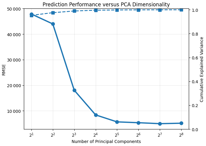
Figure 4 Sensitivity analysis of the retained PCA dimensionality for electrical power prediction using the SimpleMLP architecture. The solid line with circular markers shows the root-mean-squared error (RMSE in Watts; left axis), while the dashed line with square markers shows the cumulative explained variance (right axis) as a function of the number of retained principal components. Results are reported for the first GroupKFold validation split.

Prediction error decreases rapidly as additional principal components are retained, particularly between 4 and 32 components. Although the cumulative explained variance already exceeds 95 % with only two principal components, the corresponding prediction error remains comparatively high. This indicates that a high proportion of explained input variance does not necessarily correspond to sufficient predictive information for the target variable.

Beyond approximately 64 principal components, further reductions in RMSE become progressively smaller as the cumulative explained variance approaches 100 %. The lowest RMSE was obtained using 128 principal components, while increasing the dimensionality to 256 components provided no further improvement. This suggests that the information most relevant to electrical power prediction is captured within a comparatively compact subset of the PCA representation.

To complement the quantitative sensitivity analysis, Figs. 5 and 6 show representative reconstructions of the rotor-plane inflow fields using increasing numbers of retained principal components. Each reconstruction was obtained by projecting the original 1800-dimensional input onto the PCA basis, retaining the first n principal components, and applying the inverse PCA transformation.

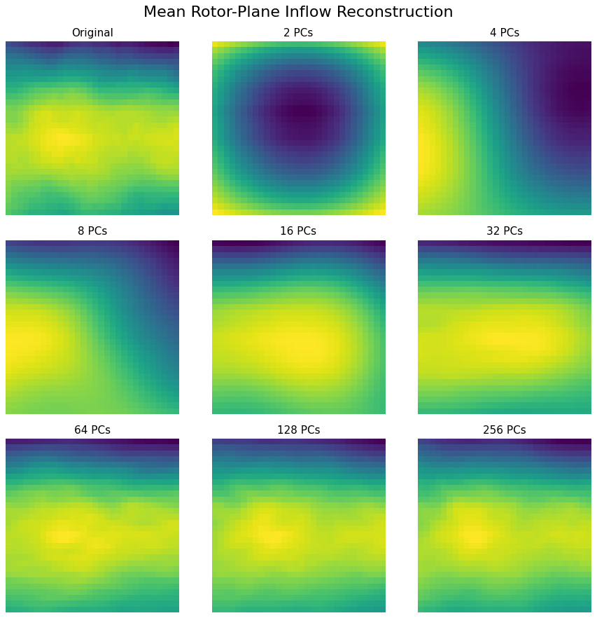
Figure 5 Reconstruction of a representative temporally aggregated mean rotor-plane inflow field using increasing numbers of retained principal components.

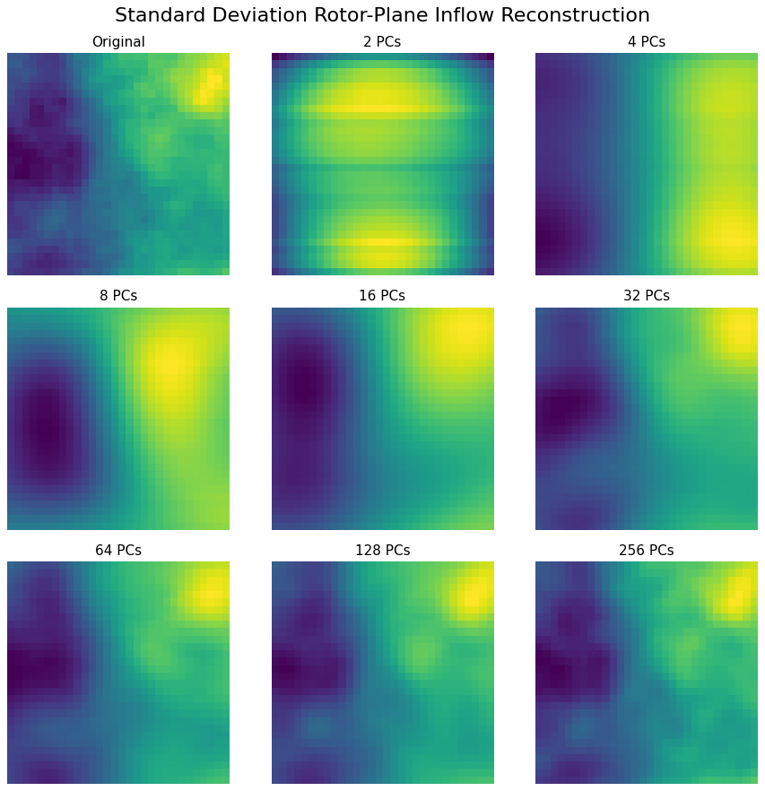
Figure 6 Reconstruction of a representative temporally aggregated standard-deviation rotor-plane inflow field using increasing numbers of retained principal components.

As the number of retained principal components increases, the reconstructed fields progressively recover the dominant characteristics of the original inflow. The large-scale structure of both the mean and standard-deviation fields is recovered using relatively few components, while additional components progressively restore finer spatial variation. Reconstructions obtained using 128 principal components are visually close to the original sample, whereas retaining 256 components results in only minor additional qualitative changes.

This behaviour is consistent with the prediction results in Fig. 4, where performance improves rapidly with increasing dimensionality before approaching a plateau near 128 components. The reconstruction therefore provides a qualitative illustration of the diminishing returns obtained by retaining additional principal components beyond this point.

Based on these results, a 128-component PCA representation was selected for the subsequent comparative evaluation. Although the detailed sensitivity analysis presented here focuses on electrical power prediction, an equivalent analysis was also performed for fatigue-load prediction. Similar saturation behaviour was observed. When comparing 128 and 256 retained components, six of the 12 fatigue-load channels achieved slightly lower prediction errors with 128 components, while the remaining six performed slightly better with 256 components. As neither dimensionality showed a consistent advantage across the fatigue-load targets, 128 components were adopted for both prediction tasks to maintain a common experimental configuration.

The resulting 128-component PCA representation was subsequently supplied to the same SimpleMLP architecture used for the full flattened-grid and baseline configurations, allowing the vector-based input representations to be compared without changing the model class.

7 Results for electrical power prediction

This section presents the predictive performance of the evaluated surrogate models for electrical power prediction. Performance is reported using the root-mean-squared error (RMSE), mean absolute error (MAE), and coefficient of determination (R²), averaged across the five GroupKFold validation folds. The corresponding mean and standard deviation values are summarised in Table 2, while Fig. 7 provides a visual comparison of the prediction errors for the principal non-baseline configurations.

Table 2 Performance comparison for electrical power prediction. Reported values correspond to the mean and standard deviation across the five GroupKFold validation folds. RMSE and MAE are reported in kW and additionally as a percentage of the turbine's rated power of 2.3 MW. The baseline, full flattened-grid, and PCA configurations are evaluated using the same SimpleMLP architecture, providing the principal fixed-architecture comparison of input representations. The ResMLP provides an additional architectural comparison using the baseline and full-grid inputs, while the CNN is reported separately as a topology-aware modelling configuration. Lower RMSE and MAE indicate better predictive performance, whereas higher R² values are preferred. Bold font indicates the configuration achieving the lowest RMSE.

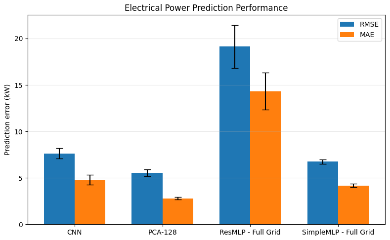
Figure 7 Comparison of electrical power prediction performance for the principal surrogate configurations. RMSE and MAE are reported in kW. Error bars denote 1 standard deviation across the five GroupKFold validation folds.

The minimal-information baseline representation produced larger prediction errors than the corresponding distributed-input configurations, but the absolute error remained small relative to the turbine's rated power. For the SimpleMLP, reducing the rotor-plane inflow to the two-variable baseline increased RMSE from 6.756 to 51.184 kW. Although this corresponds to a large relative increase with respect to the full-grid error, the baseline RMSE represents only approximately 2.225 % of the turbine's 2.3 MW rated power, and the corresponding R² remained high at 0.9966. A similar pattern was observed with the ResMLP, for which the baseline RMSE was 51.697 kW, or approximately 2.248 % of rated power. These results indicate that the two spatially aggregated quantities already capture most of the information required for electrical power prediction, while retaining distributed rotor-plane information allows the remaining prediction error to be reduced further.

Within the fixed-architecture comparison using the SimpleMLP, the PCA representation achieved the lowest prediction error. Relative to the full flattened-grid input, reducing the input dimensionality from 1800 variables to 128 principal components decreased RMSE from 6.756 to 5.534 kW, corresponding to an improvement of approximately 18.1 %. MAE was similarly reduced from 4.176 to 2.791 kW. Relative to rated power, the PCA configuration achieved an RMSE of approximately 0.241 % and an MAE of approximately 0.121 %. Because both configurations employ the same SimpleMLP architecture, this improvement is primarily associated with the change in input representation rather than to a difference in model class. The result indicates that substantial dimensionality reduction can retain the information most relevant to electrical power prediction while removing redundant or less useful variations from the original high-dimensional input.

The ResMLP produced substantially larger prediction errors than the SimpleMLP when both architectures were supplied with the same full flattened-grid representation. The full-grid ResMLP achieved an RMSE of 19.146 kW, compared with 6.756 kW for the SimpleMLP. Increasing the depth and representational capacity of the fully connected architecture therefore did not improve electrical power prediction for the full flattened input, indicating that the performance of the SimpleMLP is not simply a consequence of insufficient architectural capacity.

The topology-aware CNN achieved an RMSE of 7.636 kW and an MAE of 4.796 kW, corresponding to approximately 0.332 % and 0.209 % of rated power respectively. Its prediction error was higher than that of both the full-grid SimpleMLP and the PCA-SimpleMLP configuration, while remaining substantially lower than that of the full-grid ResMLP. Because the CNN differs from the fully connected models in both the structure of its input and its architectural inductive bias, this comparison is not interpreted as an isolated effect of input representation. Rather, the result shows that the evaluated topology-aware spatial configuration did not provide the lowest prediction error for electrical power prediction.

The richer distributed-input configurations all achieved coefficients of determination exceeding R²=0.9995, indicating that they accurately captured the overall variability in the electrical power target. The baseline configurations also retained high R² values of approximately 0.9965–0.9966 because the overall dynamic range of electrical power is large; however, their larger RMSE and MAE demonstrate that R² alone provides limited discrimination between the configurations considered here. The error-based metrics therefore provide a more informative basis for comparing predictive accuracy in the present analysis.

8 Results for fatigue prediction

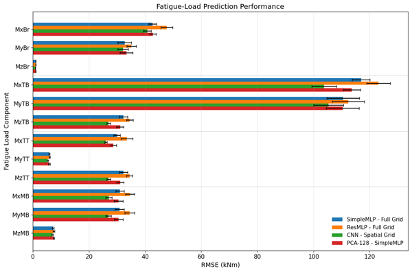
This section presents the predictive performance of the evaluated surrogate configurations for the 12 fatigue-load components. Performance is primarily assessed using the root-mean-squared error (RMSE), averaged across the five GroupKFold validation folds. The corresponding mean and standard deviation values are summarised in Table 3, while Fig. 8 provides a visual comparison of the RMSE obtained for the non-baseline configurations.

Table 3 Comparison of RMSE for the 12 fatigue-load components. Reported values correspond to the mean and standard deviation across the five GroupKFold validation folds. All RMSE values are reported in kNm. The baseline, full flattened-grid, and PCA configurations are evaluated using the same SimpleMLP architecture, permitting a fixed-architecture comparison of input representations. The ResMLP uses the full flattened-grid input, while the CNN is reported separately as a topology-aware spatial configuration. The ResMLP baseline is omitted because the baseline serves only as a minimal-information reference and its substantially poorer performance is already established under the SimpleMLP comparison. The lowest RMSE for each component is highlighted in bold.

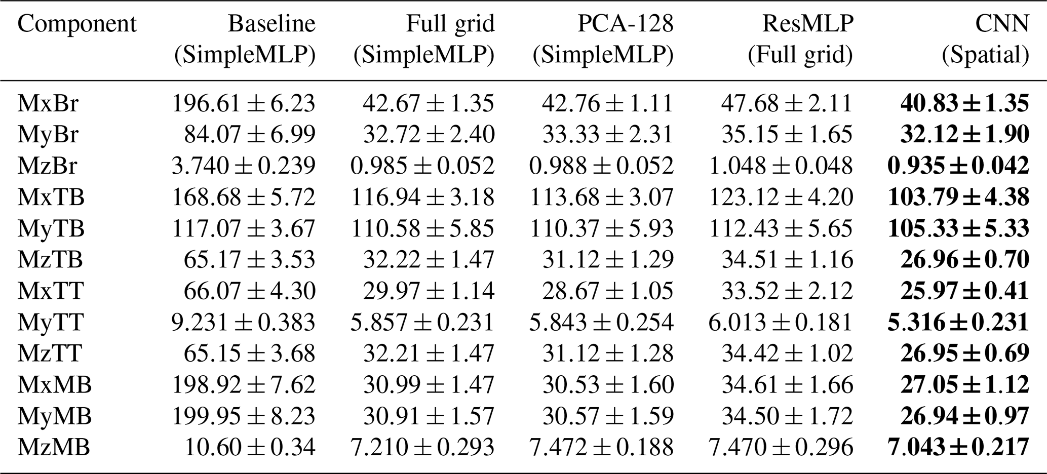
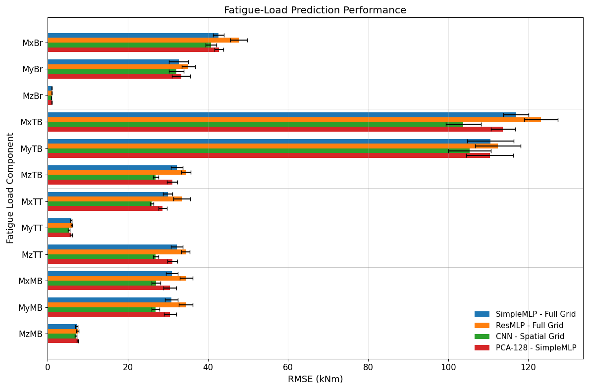
Figure 8 Comparison of RMSE across the 12 fatigue-load components for the principal non-baseline surrogate configurations. RMSE is reported in kNm. Error bars denote 1 standard deviation across the five GroupKFold validation folds. Horizontal separators distinguish blade-root, tower-base, tower-top, and main-bearing load components.

The effect of reducing the distributed rotor-plane inflow to the two-variable baseline was strongly dependent on the fatigue-load channel. For blade-root edgewise bending (MxBr), the SimpleMLP RMSE increased from 42.67 kNm with the full-grid representation to 196.61 kNm with the baseline, corresponding to degradation of a factor of approximately 4.6. An even larger effect was observed for the main-bearing bending components: MxMB increased from 30.99 to 198.92 kNm and MyMB from 30.91 to 199.95 kNm, corresponding to factors of approximately 6.4 and 6.5 respectively. By contrast, tower-base fore–aft bending (MyTB) showed only a marginal improvement when distributed inflow information was retained, with RMSE decreasing from 117.07 kNm for the baseline to 110.58 kNm for the full-grid representation.

This strong channel dependence is physically consistent with the different loading mechanisms represented by the fatigue targets. Load components dominated primarily by rotor-integrated thrust are largely captured by rotor-averaged inflow quantities, whereas components that are more sensitive to asymmetric rotor loading depend more strongly on the distributed structure of the inflow across the rotor plane. Accordingly, tower-base fore–aft bending (MyTB) improved only marginally when the distributed input was retained, whereas blade-root edgewise bending and the main-bearing bending channels improved by approximately factors of 5 and 6 respectively. This pattern is consistent with the expected dependence of fatigue-load prediction on spatial inflow information reported by Liew et al. (2023a). The baseline results therefore show that the value of distributed inflow information is strongly load-channel dependent rather than uniform across the 12 fatigue targets.

Within the fixed SimpleMLP architecture, the PCA and full flattened-grid representations produced broadly similar fatigue-load prediction errors. PCA achieved slightly lower RMSE for several tower and main-bearing components, whereas the full flattened representation performed slightly better for the blade-root components and MzMB. The differences between the two representations were generally modest, indicating that the pronounced benefit of PCA observed for electrical power prediction does not extend uniformly to the fatigue-load targets.

The topology-aware CNN achieved the lowest RMSE for all 12 fatigue-load components. However, because the CNN differs from the fully connected configurations in both its spatial input structure and its architectural inductive bias, this result is not interpreted as an isolated effect of preserving spatial topology. Rather, it demonstrates that, among the evaluated representation–architecture configurations, the spatial CNN provided the most accurate fatigue-load predictions across all 12 channels.

The full-grid ResMLP produced larger prediction errors than the corresponding full-grid SimpleMLP for all 12 fatigue-load components. Increasing the depth and representational capacity of the fully connected architecture therefore did not improve fatigue-load prediction when the same flattened input representation was retained.

Taken together with the electrical-power results, the fatigue-load results demonstrate a task-dependent pattern in the relative performance of the evaluated configurations. PCA provided a clear advantage over the full flattened input for electrical power prediction under the fixed SimpleMLP architecture, whereas the same two representations performed similarly for fatigue-load prediction. In contrast, the topology-aware CNN produced the lowest errors across all fatigue-load components but did not provide the lowest error for electrical power. The preferred representation–architecture configuration among those evaluated therefore depends on the prediction objective.

9 Discussion

This study investigated how the amount and form of retained rotor-plane inflow information influence surrogate modelling performance for electrical power and fatigue-load estimation. The baseline comparison revealed a clear distinction between the two prediction tasks. For electrical power, the two spatially aggregated quantities were already close to sufficient, with the baseline SimpleMLP achieving an RMSE of only 2.225 % of rated power. Fatigue-load prediction showed a stronger and highly channel-dependent sensitivity to distributed inflow structure: thrust-dominated channels benefited comparatively little, whereas channels associated more strongly with asymmetric rotor loading benefited substantially. This pattern is consistent with the expected dependence on spatial inflow information reported by Liew et al. (2023a).

For electrical power prediction, the fixed-architecture comparison between the full flattened-grid and PCA representations showed a clear advantage for dimensionality reduction. The PCA representation achieved the lowest prediction error while reducing the input dimensionality from 1800 variables to 128 principal components. Because both configurations were evaluated using the same SimpleMLP architecture, the difference can be interpreted primarily in terms of the input representation rather than a change in model class. The accompanying PCA sensitivity analysis further showed that explained input variance alone is not a sufficient criterion for selecting the retained dimensionality: although a very small number of components already captured most of the variance in the inflow data, substantially more components were required to achieve the lowest prediction error.

Fatigue-load prediction exhibited a different pattern. Under the same SimpleMLP architecture, the full flattened-grid and PCA representations produced broadly similar errors, with neither representation showing a consistent advantage across all 12 load components. In contrast, the topology-aware CNN achieved the lowest RMSE for every fatigue-load component. Because this configuration differs from the fully connected models in both the spatial organisation of the input and the architectural inductive bias used to process that input, its superior performance cannot be attributed to spatial representation alone. Instead, the result indicates that the evaluated combination of topology-preserving input and convolutional architecture is particularly effective for fatigue-load prediction.

The comparison between the SimpleMLP and ResMLP further shows that increased architectural complexity alone did not improve predictive performance. When supplied with the same full flattened-grid representation, the deeper ResMLP produced larger errors than the SimpleMLP for both electrical power and fatigue-load prediction. This suggests that the performance differences observed among the evaluated configurations are not simply explained by model capacity.

Taken together, the results do not identify a single universally optimal input representation or model class. Rather, they show that the preferred representation–architecture configuration among those evaluated depends on the prediction objective. For electrical power prediction, the PCA-SimpleMLP configuration provided the highest accuracy among the evaluated approaches, whereas for fatigue-load prediction the topology-aware CNN achieved the lowest errors across all load components. At the same time, the baseline comparison shows that the value of distributed rotor-plane information differs substantially between the two prediction tasks and, for fatigue prediction, between individual load channels. These findings therefore support selecting the input representation and surrogate architecture jointly according to the target quantity, rather than assuming that a single representation or model class will be equally effective for both electrical power and structural-load prediction.

Limitations and practical relevance

Several limitations should be considered when interpreting the results of this study. First, the rotor-plane inflow fields used here are temporally aggregated over 10 min intervals and are represented only by the corresponding mean and standard-deviation fields. The conclusions therefore apply specifically to surrogate modelling from temporally aggregated inflow information and may not extend directly to models operating on time-resolved flow fields or representations containing additional temporal or higher-order flow statistics.

Second, the surrogate architectures considered in this study are not exhaustive. The SimpleMLP, ResMLP, and CNN provide representative fully connected and convolutional modelling approaches, but alternative architectures, including transformer-based, graph-based, or other spatial learning methods, may yield different absolute performance or alter the detailed ranking between individual models. The present results should therefore not be interpreted as establishing a universally optimal architecture or representation for either electrical power or fatigue-load prediction. Rather, they demonstrate that the relative effectiveness of the evaluated representation–architecture combinations differs between the two prediction targets considered here.

For the principal representation comparison, the baseline, flattened full-grid, and PCA-reduced inputs are evaluated using the same SimpleMLP architecture. This allows differences among these configurations to be interpreted primarily in terms of the information retained by the input representation. The CNN is considered separately as a topology-aware model that explicitly exploits the two-dimensional neighbourhood structure of the rotor-plane fields through convolutional kernels. Consequently, differences between the CNN and fully connected models should not be interpreted as the isolated effect of input representation alone but as the combined effect of spatial representation and architectural inductive bias (Lecun et al., 1998; Bronstein et al., 2021; Battaglia et al., 2018).

The intended role of the surrogate framework is not to eliminate the high-fidelity simulations required to construct its training database but to provide a computationally inexpensive response approximation once such a database has been generated. The approach therefore primarily targets simulation-based applications that require repeated evaluation of turbine power or structural loads over many inflow or operating conditions, such as wind-farm layout optimisation, flow-control studies, fatigue-aware optimisation, and large-scale parametric investigations. Previous work has demonstrated the use of surrogate models for rapid prediction of both short-term fatigue loads and electrical power in wind-farm control and optimisation studies (Gasparis et al., 2020). Simulation-trained surrogates have also been applied to rapid site-specific lifetime fatigue-load assessment (Dimitrov et al., 2018), while more recent work has demonstrated fatigue-load surrogate modelling based on simulated inflow slices for fatigue-aware wind-farm layout and flow-control optimisation (Guilloré et al., 2026).

For these simulation-based applications, the rotor-plane inflow required by the present framework would be supplied by wake or flow-field simulations evaluated at the turbine location before the corresponding aeroelastic turbine response is computed. This is consistent with recent fatigue-surrogate approaches in which libraries of simulated inflow slices are generated from wake simulations and subsequently used to drive aero-servo-elastic turbine models (Guilloré et al., 2026). In such settings, the trained surrogate can replace repeated high-fidelity turbine-response calculations while retaining inflow information supplied by a lower-cost flow model.

Operational or measurement-informed use would require an estimate of the incoming rotor-scale inflow from measurements. Nacelle-mounted lidar provides one possible source of such information: lidar measurements have been used to estimate rotor-effective wind speed and to provide information on the approaching inflow relevant to wind-turbine control (Held and Mann, 2019). Rotor-effective wind speed can also be inferred from standard turbine measurements using state-estimation approaches (Lio et al., 2023). These operational estimates are substantially less complete than the idealised full rotor-plane fields available in the present simulation dataset. In particular, measurement sparsity, spatial filtering, reconstruction assumptions, line-of-sight limitations, noise, missing observations, and wake-contaminated measurements would need to be addressed before the present framework could be transferred directly to field applications. Accordingly, the current results should be interpreted primarily as demonstrating the influence of inflow representation under controlled simulation conditions rather than as validating a deployment-ready operational surrogate.

Finally, the analysis is based on the publicly available HAWC2Farm Lillgrund simulation dataset. Although the dataset contains a large number of observations covering a broad range of simulated inflow conditions, it represents a single wind-farm configuration and does not include many sources of uncertainty encountered in field measurements, such as measurement noise, missing data, or unmodelled atmospheric variability. Previous surrogate-modelling studies have therefore highlighted the importance of evaluating simulation-derived models against operational or field measurements when assessing their applicability beyond controlled numerical datasets (Kottakat et al., 2026). Further evaluation on other turbine designs, wind-farm layouts, inflow conditions, and operational measurements would therefore be required to assess the generality of the observed trends.

10 Conclusions

This work shows that the predictive value of rotor-plane inflow information depends strongly on the target quantity. Electrical power could already be predicted relatively accurately from the two spatially aggregated baseline quantities, with distributed representations mainly serving to reduce the remaining prediction error. Fatigue-load prediction was more sensitive to the retained spatial information and, importantly, this sensitivity varied substantially between load channels. The marginal change observed for tower-base fore–aft bending contrasts with the much larger improvements for blade-root edgewise and main-bearing bending, highlighting the different information requirements of thrust-dominated and asymmetry-sensitive structural responses.

Among the richer representations, dimensionality reduction through PCA was particularly effective for electrical power prediction, providing the lowest error under the fixed SimpleMLP architecture while reducing the input dimensionality from 1800 variables to 128 principal components. For fatigue-load prediction, the full-grid and PCA representations performed similarly under the same architecture, whereas the topology-aware CNN achieved the lowest errors across all 12 load components. These results reinforce that neither a single inflow representation nor a single surrogate architecture should be assumed to be optimal across prediction objectives.

The present findings are specific to the evaluated HAWC2Farm dataset, temporally aggregated inflow representation, and surrogate architectures. Future work should therefore examine whether the same task- and channel-dependent behaviour persists across other turbine designs, wind-farm layouts, inflow conditions, and alternative spatial modelling approaches.