A novel analytical tool to capture wind profile variability for wind energy assessment: fast, simple, and beyond state-of-the-art in complex terrain

Standardized wind turbine power-performance evaluation commonly represents the vertically varying rotor inflow by a single reference wind speed, such as hub-height wind speed or rotor-equivalent wind speed. Here, we present a computationally simple analytical rotor-integration model for turbine power that evaluates the vertical variation in horizontal wind speed using a Taylor expansion of the inflow velocity over the rotor disk. We assess idealized wind profiles to understand the isolated effects of typical shear, veer profiles, and turbulence on the power production of the turbine. This analytical model is then evaluated against power measurements from five Enercon E92 turbines at Gotthard Pass, a complex-terrain wind park in the Swiss Alps, across 10 distinct wind events. The model consistently improves upon the hub-height-based reference approach and reaches an accuracy comparable to OpenFAST simulations while requiring no specialized modeling expertise to operate. It thereby provides smoother and more accurate power estimates, reducing RMSE by 8.8 % and achieving a mean reduction in absolute case-wise bias of 27.2 % relative to the hub-height-based reference approach across the evaluated wake-free cases. These improvements apply to the investigated events. Additionally, it enables effective filtering of wake-affected lidar measurements, demonstrating flexibility, robustness, and applicability for pre-construction assessment and wind park expansion in complex terrain.

1 Introduction

Accurate modeling of wind turbine power generation requires more than the direct application of hub-height power curves. Standard power curves, as defined in IEC 61400-12-1, provide a well-established framework based on mean wind speed at hub height, but they only partly represent the atmospheric complexity that can influence power production (IEC, 2022; Sakagami et al., 2015). Remaining uncertainties are closely linked to wind variability, turbulence, and boundary-layer processes, whose effects become increasingly important as turbine size increases (Belu and Koracin, 2012).

Although multi-height wind measurements from meteorological masts and Doppler-wind lidar are widely used and included in international standards, power performance assessments typically reduce the vertically varying inflow across the rotor-swept area to a single representative wind speed. This value is usually derived from a nacelle-mounted anemometer calibrated against the kinetic energy flux measured across the rotor plane approximately 2.5 rotor diameters upstream (IEC, 2022). While appropriate for standardized test sites with flat or mildly complex terrain, this approach assumes quasi-uniform inflow across the rotor disk. In complex terrain, however, strong vertical and lateral gradients caused by wind shear, directional veer, turbulence, yaw misalignment, and wake effects violate this assumption, leading to increased uncertainty in power-curve application.

Turbulence intensity strongly influences measured power curves, as standard 10 min averaging obscures short-term variability and complicates comparisons with guaranteed performance (Albers, 2010). Wind shear and directional veer further modify the effective inflow, such that alignment with hub-height wind may lead to sub- or super-optimal power production depending on the vertical profile (Murphy et al., 2020). These effects are amplified in complex terrain, where non-homogeneous upstream flow alters wake development and induction compared to flat, homogeneous conditions (Troldborg et al., 2022; Gasser et al., 2026). Despite these limitations, the reduction in spatially varying inflow to a single-point wind speed remains the prevailing standard for consistency in power assessment (IEC, 2022).

In recent years, simulations and analytical approaches that explicitly account for spatial wind velocity distributions have gained attention for their ability to capture key processes influencing turbine power output. Modified power-curve and induction models incorporating wind shear, veer, turbulence intensity, and yaw misalignment improve power prediction accuracy by up to 51 % (Vahidzadeh and Markfort, 2019, 2020). Similarly, coupling actuator disk theory with blade-element models to resolve vertical shear and directional changes improves agreement with observed turbine power and reduces prediction errors (Mata et al., 2024). At the wind farm scale, Gaussian process and random forest approaches further highlight the importance of accounting for wake-induced turbulence and vertical profile variability, showing good agreement with large-eddy simulations and observations (Niayifar and Porté-Agel, 2015; Clifton and Wagner, 2014).

Early power-performance studies showed that the sensitivity of measured power curves to atmospheric conditions partly reflects limitations in the reference wind speed definition. Using multi-level measurements across the rotor layer, Elliott and Cadogan (1990) demonstrated that stratifying power curves by turbulence intensity yields substantially different outputs at identical hub-height wind speeds, largely due to systematic deviations between hub-height and disk-averaged wind speeds under low-turbulence, strongly sheared conditions. In such regimes, hub-height wind speed frequently overestimates disk-averaged velocity, indicating that single-point measurements can bias the inferred kinetic input and distort interpretations of power-curve scatter and apparent underperformance (Elliott and Cadogan, 1990).

Motivated by these findings, several studies proposed replacing hub-height wind speed with an equivalent or rotor-averaged wind speed that better represents rotor-integrated inflow. Simulation studies over flat terrain showed that electrical power correlates more strongly with rotor-equivalent wind speed (REWS), derived from measurements across the swept area, than with hub-height wind speed, highlighting that identical hub-height values can correspond to substantially different rotor-layer kinetic energy (Wagner et al., 2009). A widely adopted formulation defines REWS by matching the kinetic energy flux through the rotor, resulting in a cubic (energy-based) rotor-area weighting:

$$\begin{array}{}\text{(1)}& U_{\mathrm{eq}}={\left(\sum _i{u}_i^{\mathrm{3}}{\displaystyle \frac{A_i}{A}}\right)}^{\mathrm{1}/\mathrm{3}},\end{array}$$

where u_i represents the wind speed measured within rotor-area segment i, A_i is the area of that segment, and A is the total rotor-swept area. In lidar-based applications, this energy-equivalent definition reduces power-curve scatter and yields a power coefficient consistent with the profile-integrated kinetic energy flux, rather than the hub-height approximation (Wagner et al., 2011).

As rotor-equivalent wind speed methods gained wider adoption, their practical implementation became an important topic. The IEA Wind Annex 32 comparative exercise showed that applying the IEC-draft REWS procedure requires explicit choices in assigning rotor-area weights to discrete measurement heights, including the definition of segment areas and the treatment of measurements not located at rotor-tip elevations. Even for identical wind profiles, small but systematic differences in REWS were found across institutions due solely to variations in the segmentation and weighting approach, highlighting that REWS is not only a concept but also a method affecting reproducibility. The same study further showed that REWS-based power curves can differ substantially from hub-height-based curves, particularly under strong shear and low-turbulence conditions, where inflow non-uniformity is most pronounced (Wagner et al., 2014).

Beyond shear-only corrections, several studies proposed veer- and turbulence-aware rotor-equivalent formulations to better represent the wind component normal to the rotor plane and its variability. In industry practice, “veer-aware” equivalent wind speeds apply a cosine projection of directional differences across the rotor, effectively down-weighting misaligned inflow (Antoniou et al., 2013). Choukulkar et al. (2016) developed an equivalent wind speed that combines rotor-area weighting with wind speed and direction variability, accounting for turbulence intensity, directional shear, and flow misalignment. Similarly, Redfern et al. (2019) introduced a momentum-based rotor-equivalent wind speed with a veer correction by projecting wind vectors onto the turbine axis.

Field measurements confirm that intra-rotor flow variability can lead to substantial deviations from standard power curves. Combinations of wind shear and directional veer can induce power changes ranging from −19 % to +34 % relative to the nominal curve at a given hub-height wind speed (Mata et al., 2024). Differences between hub-height wind speed and REWS can exceed 70 kW, corresponding to up to 5 % of rated power for a single turbine (Murphy et al., 2020). These discrepancies can propagate to the wind farm scale and may lead to significant instantaneous and cumulative power prediction errors, although their aggregate effect depends on how errors vary across turbines.

Ground-based Doppler wind lidar enables retrieval of wind speed and direction profiles across the rotor-swept area, allowing equivalent wind speeds to be derived based on kinetic energy flux rather than single-point measurements (Wagner et al., 2011). Although IEC 61400-12-1 acknowledges that non-uniform inflow, including shear and turbulence across the rotor, can bias power-performance measurements, standardized procedures primarily express these effects through weighted or equivalent reference wind speeds for power-curve evaluation (IEC, 2022). This provides a reproducible basis for certification and comparison but leaves room for complementary analytical formulations that explicitly decompose how shear, veer, turbulence, and yaw misalignment affect the rotor-integrated power input, especially in complex terrain.

The benefit of adopting REWS over hub-height wind speed is not universal, as both can differ by less than 1 % under homogeneous conditions with weak shear, implying limited added value in such cases. However, larger deviations occur in complex terrain and atypical shear regimes, supporting the view that REWS-based normalization is most relevant where strong, non-linear shear and veer are frequent conditions typical of mountainous wind parks and central to this study (Van Sark et al., 2019).

Building on this established body of work, the present study does not aim to introduce rotor-equivalent wind speed or rotor-integrated inflow concepts as new. Instead, we develop a computationally simple analytical formulation that evaluates wind turbine power generation directly as an integral over the rotor-swept area. The formulation retains the physical interpretation of rotor-integrated kinetic energy while allowing the separate and combined effects of vertical shear, directional veer, turbulence intensity, and yaw misalignment to be evaluated explicitly. The contribution of the study therefore lies in the specific analytical implementation, its comparison against numerical simulations under controlled inflow conditions, and its application to lidar-derived wind profiles from a mountainous site.

To evaluate the proposed analytical approach, we use numerical simulations from OpenFAST, an open-source wind turbine model developed by the National Laboratory of the Rockies (NRL), formerly known as the National Renewable Energy Laboratory (NREL) (Jonkman, 2013), which resolves turbine dynamics under spatially and temporally varying inflow and captures the intra-rotor flow structure considered here. The observational analysis focuses on the complex-terrain Gotthard Pass in the Swiss Alps. During a field campaign, wind profiles were measured using lidar, providing observations of vertically variable flow conditions relevant for wind turbine power estimation in complex terrain.

This article is structured as follows. Section 2 summarizes the established theoretical and experimental background needed for the study, including rotor-equivalent wind speed concepts, the turbine power equation, turbulence notation, the Gotthard field site, and the OpenFAST/TurbSim framework. Section 3 then describes the specific implementation developed here: the Taylor-series rotor integration, the power-curve and power-coefficient retrieval, the idealized profile experiments, the OpenFAST simulations, and the application to lidar-derived Gotthard inflow profiles. The results in Sect. 4 then compare the analytical estimates with the numerical simulations and measured turbine power to assess when vertical profile information improves power prediction in complex terrain.

2 Background and theoretical framework

This section summarizes the established concepts and data sources on which the present method is built. The material is separated from the implementation of the proposed method so that the analytical assumptions, site information, and numerical modeling framework are introduced before the workflow used in this study.

2.1 Rotor-equivalent wind speed, turbine power, and vertical inflow variability

The standard wind turbine power equation can be written as

$$\begin{array}{}\text{(2)}& P\left(U_{\mathrm{eq}}\right)={\displaystyle \frac{\mathrm{1}}{\mathrm{2}}}{C}_{\mathrm{p}}\left(U_{\mathrm{eq}}\right)\mathit{\rho }A{U}_{\mathrm{eq}}^{\mathrm{3}},\end{array}$$

where P is the turbine power output, U_eq is a representative rotor-equivalent wind speed, C_p is the power coefficient, ρ is air density, and A=πR² is the rotor-swept area with rotor radius R. In the simplest interpretation, U_eq is represented by the hub-height wind speed. In rotor-equivalent wind speed approaches, however, U_eq is instead derived from the kinetic-energy flux through the rotor-swept area, for example using Eq. (1).

Equation (2) is therefore not introduced here as a new model, but as the basis from which rotor-integrated approaches follow. The contribution of this study is to retain the rotor-integrated interpretation while expressing the vertical inflow profile as an analytical function. This makes it possible to decompose the effects of shear, veer, and turbulence without reducing all inflow variability to a single scalar wind speed at the start of the calculation.

Figure 1 Vertical integration over the rotor-swept area of a wind turbine.

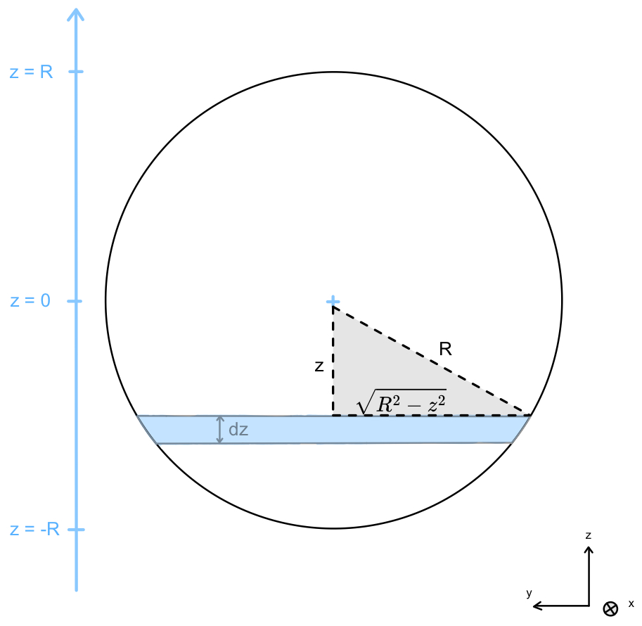
As shown in Fig. 1, the coordinate z is defined relative to the turbine hub, with z=0 at hub height and $z=-R$ and z=R at the lower and upper rotor tips. A vertical profile v(z) therefore describes the horizontal wind speed magnitude sampled through the rotor layer. Directional veer is treated by projecting the wind vector onto the rotor-normal direction before applying the same vertical integration.

In complex terrain, wind velocity varies across the rotor-swept area due to terrain-induced acceleration, directional channeling, vertical shear, turbulence, and wake effects. In undisturbed boundary-layer flow, vertical variations are generally more important than horizontal variations across the rotor disk because vertical gradients in wind speed and direction are a dominant feature of the surface layer and lower boundary layer (Stull, 1988; Wagner et al., 2014; IEC, 2022). This assumption does not necessarily hold inside turbine wakes or in strongly heterogeneous terrain-induced flow; wake-contaminated profiles are therefore treated separately in Sect. 4.3.

2.2 Turbulence notation

For the analytical turbulence treatment, turbulence is represented by the second-order statistics of the wind speed at each measurement height. For each height z, the 10 min wind speed distribution is described by a mean $\stackrel{\mathrm{‾}}{v}\left(z\right)$ and standard deviation σ_v(z). These are not rotor-equivalent quantities; they are height-dependent statistics derived from the measured or prescribed wind speed time series. The latter is derived directly from the WindCube lidar wind speed dispersion parameter as described in VAISALA (2023).

In the analytical implementation, the probability density function modeling the distribution of instantaneous wind speed values at height z is approximated by a Gaussian distribution,

$$\begin{array}{}\text{(3)}& f_z\left(V\right)={\displaystyle \frac{\mathrm{1}}{\sqrt{\mathrm{2}\mathit{\pi }{\mathit{\sigma }}_v(z{)}^{\mathrm{2}}}}}\exp \left[-{\displaystyle \frac{{\left(V-\stackrel{\mathrm{‾}}{v}\left(z\right)\right)}^{\mathrm{2}}}{\mathrm{2}{\mathit{\sigma }}_v(z{)}^{\mathrm{2}}}}\right],\end{array}$$

where V denotes the instantaneous wind speed used as the integration variable. The Gaussian assumption is used here as a controlled second-order representation of turbulent wind speed variability. Rather than attempting to reproduce all higher-order or non-Gaussian features of atmospheric turbulence, it provides a reproducible and analytically tractable formulation that can be directly combined with the turbine power curve.

It has been shown by van Schaik et al. (2025b) that heavier-tailed wind speed distributions, such as Student's t distribution, are commonly observed at Gotthard Pass. In the present formulation, however, turbulence is represented through a single standard-deviation measure. Within this second-order framework, the effect of heavier tails can be incorporated through a simple scaling of the wind speed standard deviation by a factor of 1.81, which effectively captures their influence on turbine power output (van Schaik et al., 2025b).

2.3 Gotthard field site and observations

The observational evaluation uses the Gotthard Wind Park in the central Swiss Alps. The wind farm is located at 2106 m a.m.s.l. on the north–south-oriented Gotthard Pass and consists of five Enercon E92 wind turbines with a rated power of 2.35 MW, a hub height of 98 m, and a rotor diameter of 92 m. Real-condition wind power output and nacelle wind speed data at 10 min resolution were taken from van Schaik et al. (2025b).

During the Gotthard transect campaign, Doppler wind lidar measurements were collected at several locations around the wind farm. The lidar measured vertical profiles of wind speed, wind direction, and wind speed variability at 10 min resolution, with measurement heights of 40–150 m in 10 m increments and 160–300 m in 20 m increments. For the Enercon E92 rotor layer, this typically provides six to nine measurement gates within the rotor-swept area, depending on the lidar location and local elevation difference relative to the turbine base.

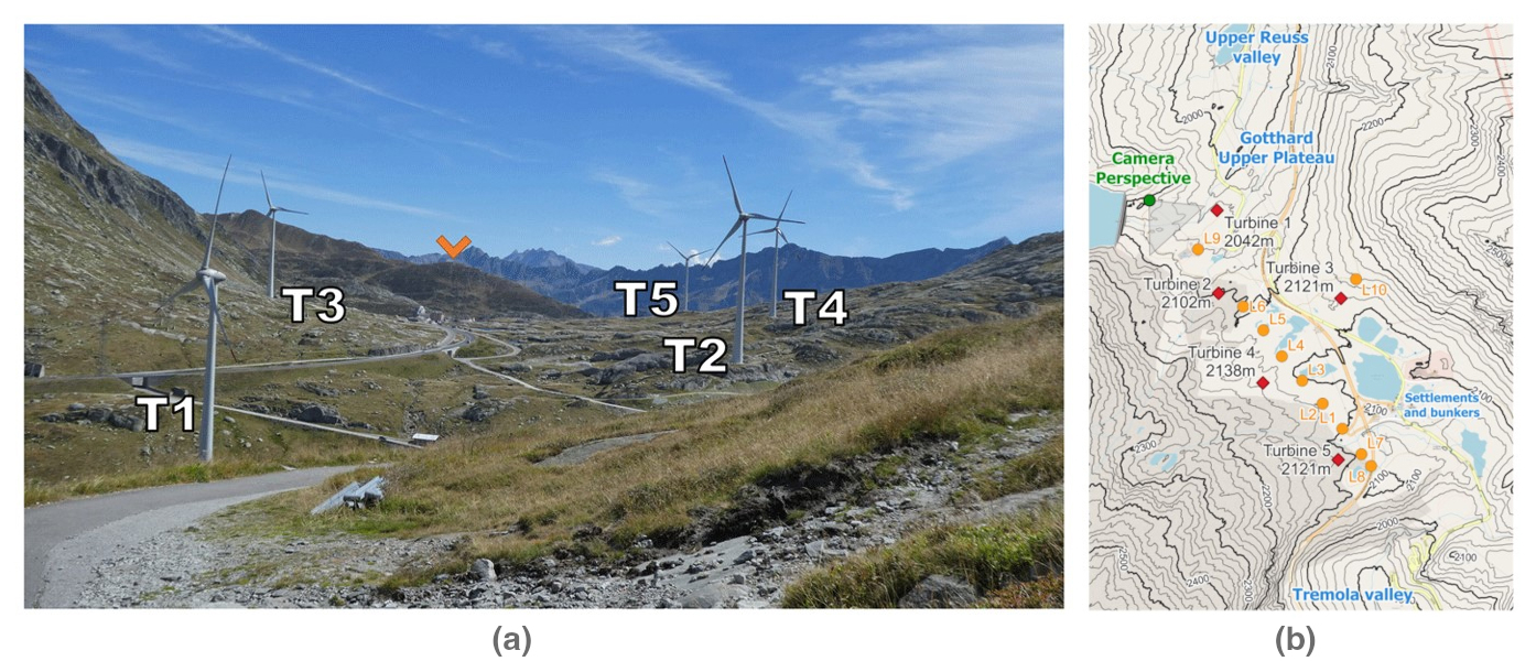
Figure 2 Turbine and lidar locations from the Gotthard Doppler wind lidar campaign in summer 2023, adapted from van Schaik et al. (2025b).

2.4 OpenFAST and TurbSim background

OpenFAST is used as a numerical reference framework to test the analytical formulation under controlled inflow conditions. Because the detailed blade geometry and controller configuration of the Enercon E92 are proprietary, the simulations use the open-source WindPACT 3.0 MW reference turbine. This introduces a known limitation: differences between the Enercon E92 and WindPACT power curves can affect the comparison independently of the inflow-integration method.

TurbSim is used to generate the turbulent inflow fields required by OpenFAST. Non-turbulent simulations use deterministic, user-defined vertical wind profiles without turbulent fluctuations. For the turbulent Gotthard comparison, the user-defined von Kármán option (USRVKM) is used because it allows the measured height-dependent mean wind speed, wind direction, and wind speed standard-deviation profiles to be retained directly in the numerical inflow. USRVKM additionally requires an integral length-scale profile and component scaling, which are specified as described in Sect. 3.5.

3 Methodology

This section describes the implementation used in this study. Section 3.1 introduces the analytical rotor integration, Sect. 3.2 describes power-curve fitting and power-coefficient retrieval, Sect. 3.3 presents the analytical turbulence treatment, Sect. 3.4 defines the idealized profile experiments, Sect. 3.5 describes the OpenFAST simulations, and Sects. 3.6 and 3.7 explain the Gotthard application and model evaluation.

3.1 Analytical rotor integration

To account for vertical variations in horizontal wind speed, the power input is integrated over horizontal rotor slices, as shown in Fig. 1. The width of a slice at height z is $\mathrm{2}\sqrt{R^{\mathrm{2}}-z^{\mathrm{2}}}$, giving

$$\begin{array}{}\text{(4)}& P_{\mathrm{an}}={\displaystyle \frac{\mathrm{1}}{\mathrm{2}}}{C}_{\mathrm{p}}\left(U_{\mathrm{eq}}\right)\mathit{\rho }\underset{-R}{\overset{R}{\int }}\mathrm{2}\sqrt{R^{\mathrm{2}}-z^{\mathrm{2}}}v(z{)}^{\mathrm{3}}\mathrm{d}z.\end{array}$$

Here, v(z) is the vertical profile of horizontal wind speed after any required vector projection onto the rotor-normal direction. The power coefficient is evaluated at the rotor-equivalent wind speed corresponding to the same profile, not independently at each height.

The measured or idealized profile is represented by a Taylor polynomial of order N,

$$\begin{array}{}\text{(5)}& v\left(z\right)=\sum _{i=\mathrm{0}}^N{c}_{v,i}{z}^i=c_{v,\mathrm{0}}+c_{v,\mathrm{1}}z+c_{v,\mathrm{2}}{z}^{\mathrm{2}}+\mathrm{\dots }+c_{v,N}{z}^N.\end{array}$$

The notation c_v,i is used to distinguish the Taylor coefficients of the mean wind speed profile from the turbulence-profile coefficients introduced in Sect. 3.3. In the present study, N=3 is used as a compromise between flexibility and overfitting. The same order is used for all measured and idealized profiles unless stated otherwise.

Substituting Eq. (5) into Eq. (4) gives an analytical expression for the rotor-integrated power,

$$\begin{array}{}\text{(6)}& \begin{array}{rl}{P}_{\mathrm{an}}& ={\displaystyle \frac{\mathrm{1}}{\mathrm{2}}}{C}_{\mathrm{p}}\left(U_{\mathrm{eq}}\right)\mathit{\rho }A\sum _{i,j,k=\mathrm{0}}^N{c}_{v,i}{c}_{v,j}{c}_{v,k}{R}^m{K}_m,\\ & m=i+j+k,m\mathrm{even},\end{array}\end{array}$$

with

$$\begin{array}{}\text{(7)}& K_m={\displaystyle \frac{m\mathrm{!}}{{\mathrm{2}}^m{\left[(m/\mathrm{2})\mathrm{!}\right]}^{\mathrm{2}}(m/\mathrm{2}+\mathrm{1})}}.\end{array}$$

Odd values of m do not contribute because the corresponding terms integrate to zero over the symmetric rotor interval. The full derivation is provided in Appendix A. In the code implementation, the workflow first fits c_v,i from the available height levels and then evaluates Eq. (6) exactly through the triple summation.

3.2 Power-curve fitting and power-coefficient retrieval

The analytical model requires both a continuous turbine power curve and the corresponding power coefficient. The turbine power curve is represented by

$$\begin{array}{}\text{(8)}& P_{\mathrm{pc}}\left(U\right)=P_{\mathrm{r}}\left[\mathrm{1}-\exp \left(-{\left({\displaystyle \frac{U-v_{\mathrm{in}}}{C}}\right)}^B\right)\right],\end{array}$$

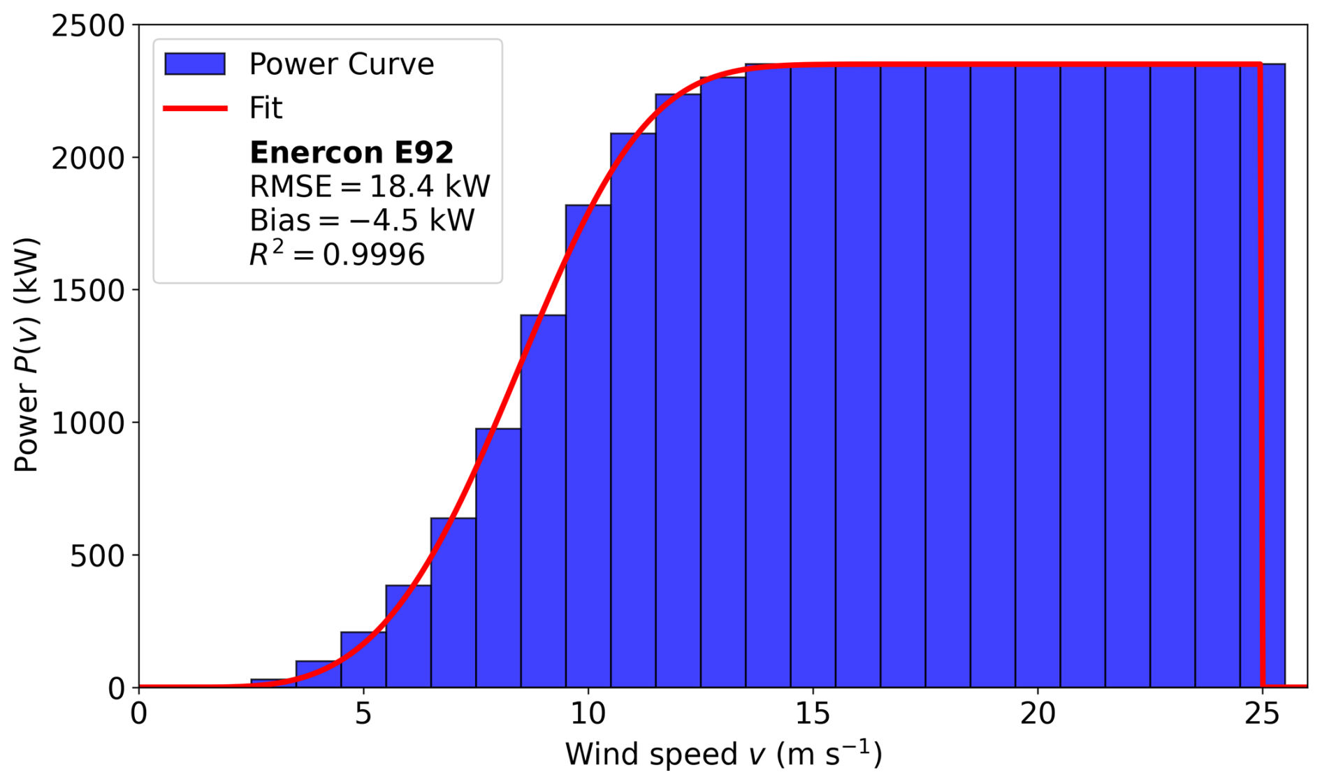
where U denotes the scalar reference wind speed at which the turbine power curve is evaluated; in the rotor-integrated analytical calculations, it is set to U_eq. For $v_{\mathrm{in}}\le U\le v_{\mathrm{out}}$, P_pc is given by Eq. (8), with P_pc=0 below cut-in and above cut-out and P_pc=P_r in the rated-power region where applicable. The fixed parameters v_in, v_out, and P_r are taken from the turbine technical specifications (wind-turbine-models.com, 2026). The shape parameters B and C are fitted to the published power-curve table, which results in the fit of Fig. 3, which gives excellent agreement with the tabulated manufacturer power curve.

Figure 3 Fitting of Eq. (8) to the Enercon E92 2.35 MW turbine.

After fitting P_pc(U), the corresponding power coefficient is computed as

$$\begin{array}{}\text{(9)}& C_{\mathrm{p}}\left(U\right)={\displaystyle \frac{\mathrm{2}{P}_{\mathrm{pc}}\left(U\right)}{\mathit{\rho }A{U}^{\mathrm{3}}}}.\end{array}$$

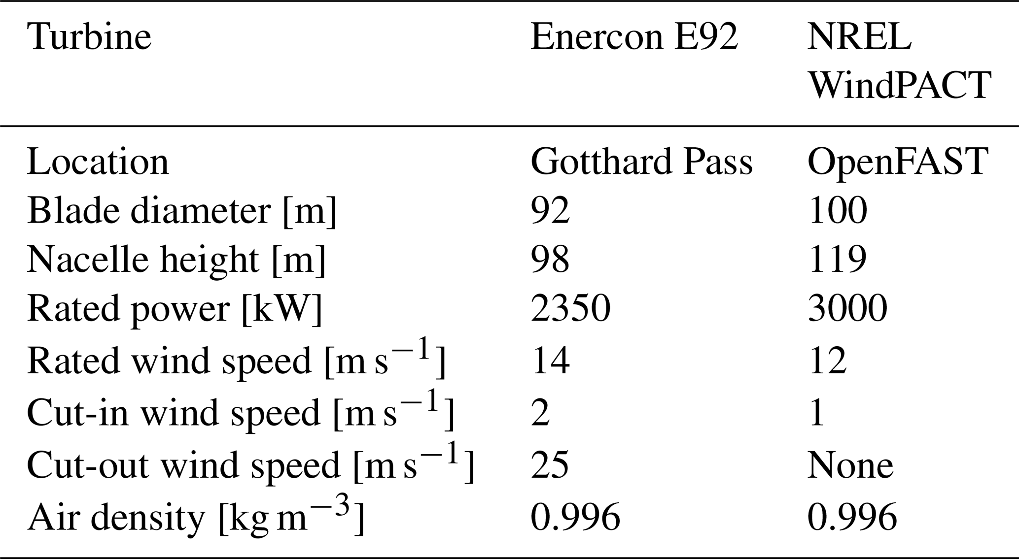
This makes the output of the power-curve-fitting step explicit: the fitted power curve P_pc(U) and the derived power coefficient C_p(U) are both passed to the analytical rotor-integration workflow. For the Gotthard application, the Enercon E92 2.35 MW power curve is used. For the OpenFAST comparison, the WindPACT 3.0 MW reference-turbine power curve is kept separate so that differences in turbine design are not confused with differences in inflow treatment. The exact specifications of both turbines can be found in Table 1.

Table 1 Specifications of the Enercon E92 and NREL WindPACT turbines in this study.

3.3 Analytical treatment of turbulence

For turbulent inflow, the mean wind speed profile is represented by the Taylor expansion in Eq. (5). The wind speed standard-deviation profile is represented by an analogous Taylor expansion over the rotor layer, using coefficients $c_{{\mathit{\sigma }}_v,i}$ instead of c_v,i:

$$\begin{array}{}\text{(10)}& {\mathit{\sigma }}_v\left(z\right)=\sum _{i=\mathrm{0}}^N{c}_{{\mathit{\sigma }}_v,i}{z}^i,\end{array}$$

where $c_{{\mathit{\sigma }}_v,i}$ represents the Taylor coefficients of the wind speed standard-deviation profile.

At each height, the expected power under turbulent wind speed fluctuations is computed by integrating the fitted turbine power curve over the local Gaussian wind speed distribution given by Eq. (3),

$$\begin{array}{}\text{(11)}& \langle P{\rangle }_z=\underset{v_{\mathrm{in}}}{\overset{v_{\mathrm{out}}}{\int }}{P}_{\mathrm{pc}}\left(V\right)f_z\left(V\right)\mathrm{d}V.\end{array}$$

The rotor-area-averaged turbulent-power estimate is then

$$\begin{array}{}\text{(12)}& P_{\mathrm{turb}}={\displaystyle \frac{\mathrm{1}}{A}}\underset{-R}{\overset{R}{\int }}\mathrm{2}\sqrt{R^{\mathrm{2}}-z^{\mathrm{2}}}\langle P{\rangle }_z\mathrm{d}z,\end{array}$$

where A=πR². The factor $\mathrm{1}/A$ is required because P_pc represents whole-turbine power. Since both $\stackrel{\mathrm{‾}}{v}\left(z\right)$ and σ_v(z) are represented by continuous Taylor expansions, 〈P〉_z is defined continuously across the rotor layer, and Eq. (12) does not require discretization into height bins.

We then refer to the contribution of turbulence to the power output of the wind turbine as the difference between this estimate and its zero-turbulence counterpart based on the same mean profile,

$$\begin{array}{}\text{(13)}& \mathrm{\Delta }{P}_{\mathrm{turb}}=P_{\mathrm{turb}}-{\displaystyle \frac{\mathrm{1}}{A}}\underset{-R}{\overset{R}{\int }}\mathrm{2}\sqrt{R^{\mathrm{2}}-z^{\mathrm{2}}}{P}_{\mathrm{pc}}\left(\stackrel{\mathrm{‾}}{v}\right(z\left)\right)\mathrm{d}z.\end{array}$$

As σ_v(z) tends to zero, 〈P〉_z tends to $P_{\mathrm{pc}}\left(\stackrel{\mathrm{‾}}{v}\right(z\left)\right)$ wherever the power curve is continuous. Consequently, ΔP_turb tends to zero, including for a nonuniform mean wind speed profile. At exactly zero turbulence, 〈P〉_z is evaluated directly as $P_{\mathrm{pc}}\left(\stackrel{\mathrm{‾}}{v}\right(z\left)\right)$.

The turbulence correction is added to the analytical mean-profile estimate to obtain $P_{\mathrm{an},\mathrm{turb}}=P_{\mathrm{an}}\left(\stackrel{\mathrm{‾}}{v}\right)+\mathrm{\Delta }{P}_{\mathrm{turb}}$. This distinction avoids ambiguity between the absolute expected power in turbulent conditions and the deviation caused by turbulence. Positive values of ΔP_turb occur mainly in the convex part of the power curve, while negative values occur where the power curve is concave.

3.4 Idealized wind profile experiments

Idealized profiles are used to isolate the effects of vertical shear, veer, turbulence, and logarithmic wind speed structure. For each experiment, both the mean wind speed profile and the turbulence profile are specified explicitly. In Fig. 4, the three different wind profiles are shown: linear-shear, linear-veer, and logarithmic profiles are first evaluated without turbulence, i.e., with σ_v(z)=0 at all heights. The logarithmic wind speed profile is written as

$$\begin{array}{}\text{(14)}& v\left(z\right)={\displaystyle \frac{u_{*}}{\mathit{\kappa }}}\ln \left({\displaystyle \frac{z_{\mathrm{h}}+z}{z_{\mathrm{0}}}}\right),\end{array}$$

where u_* is friction velocity, κ is the von Kármán constant, z_h is hub height, and z₀ is aerodynamic roughness length. This profile is used as an idealized boundary-layer case and not as a fitted site-specific roughness estimate.

The linear-shear profile is defined as $v\left(z\right)=v_{\mathrm{0}}+az$, where a=0.01, 0.025, or 0.05 s⁻¹ is the shear coefficient, and z=0 is located at turbine hub height. Relative to the uniform reference profile, the analytical power deviation is

$$\begin{array}{}\text{(15)}& \mathrm{\Delta }{P}_{\mathrm{shear}}={\displaystyle \frac{\mathrm{3}}{\mathrm{4}}}{\displaystyle \frac{R^{\mathrm{2}}{a}^{\mathrm{2}}}{v_{\mathrm{0}}^{\mathrm{2}}}}{P}_{\mathrm{ref}}.\end{array}$$

The linear-veer profile is defined by a direction that changes linearly with height, giving a rotor-normal wind speed component $v\left(z\right)=v_{\mathrm{0}}\cos ({\mathit{\alpha }}_{\max }z/R)$. Here, ${\mathit{\alpha }}_{\max }=\mathit{\alpha }R=\mathrm{5}\mathit{°}$, 10°, or 22.5° is the maximum angular deviation at the upper and lower rotor tips. Its second-order analytical power deviation is

$$\begin{array}{}\text{(16)}& \mathrm{\Delta }{P}_{\mathrm{veer}}=-{\displaystyle \frac{\mathrm{3}}{\mathrm{8}}}{\mathit{\alpha }}_{\max }^{\mathrm{2}}{P}_{\mathrm{ref}}.\end{array}$$

The homogeneous-turbulence experiment is evaluated using a uniform mean wind speed profile and constant turbulence intensity over the rotor layer. All of these wind profiles are compared to a uniform wind profile where v(z) is constant with height and σ_v(z)=0.

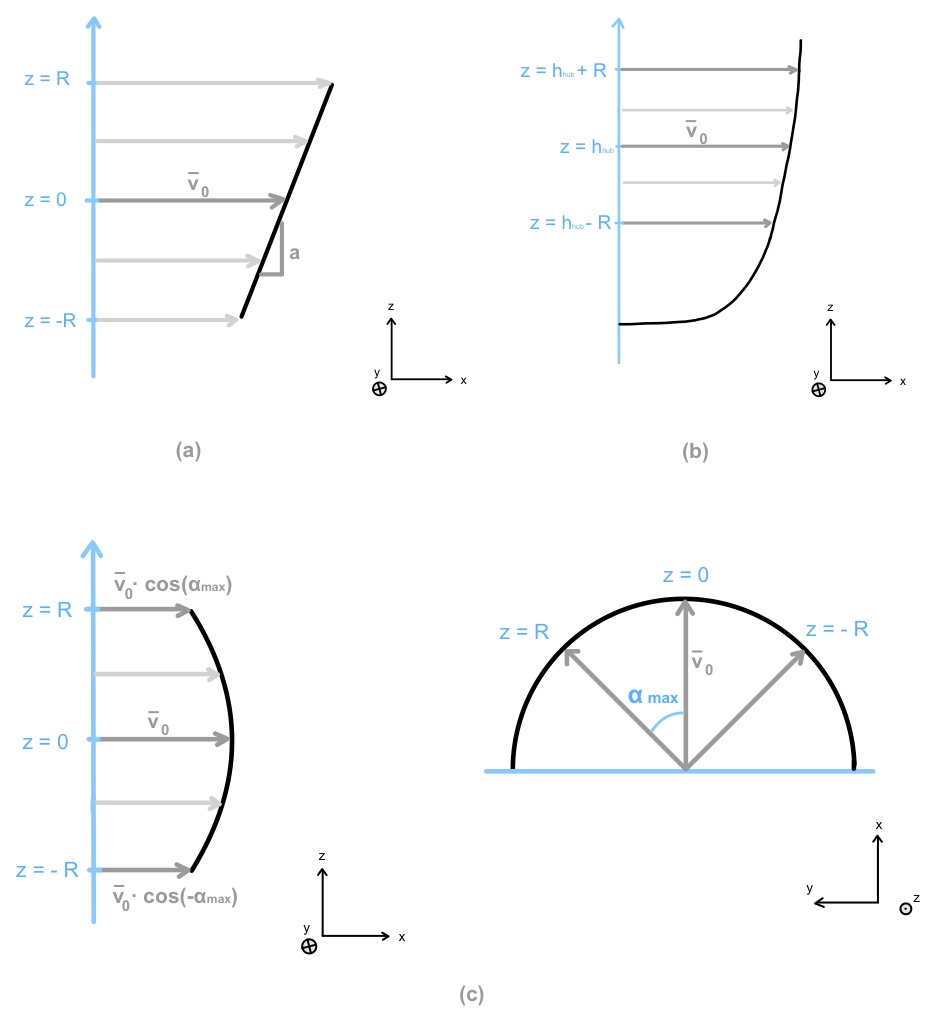
Figure 4 Examples of the idealized vertical wind profiles (a) linear shear, (b) logarithmic wind profile, and (c) linear veer.

For a given idealized profile, the analytical power deviation is computed relative to a uniform reference profile with the same hub-height wind speed,

$$\begin{array}{}\text{(17)}& \mathrm{\Delta }P=P_{\mathrm{profile}}-P_{\mathrm{ref}}.\end{array}$$

3.5 OpenFAST simulations and turbulence-model choice

OpenFAST simulations are used as a numerical reference to test whether the analytical response to prescribed vertical profiles is consistent with a higher-fidelity aeroelastic turbine model. They are not used to define the analytical formulation itself. All simulations use the WindPACT 3.0 MW reference turbine because a complete open aeroelastic model of the Enercon E92 is not available. Simulations are run for 12 min, with the first 2 min discarded as spin-up and the final 10 min used for comparison with the standard averaging interval of the lidar and turbine data.

For non-turbulent simulations, deterministic user-defined profiles are supplied without turbulent fluctuations. The idealized homogeneous-turbulence experiment uses the standard von Kármán model with prescribed constant turbulence intensity and internally determined length scales. The turbulent Gotthard simulations use the TurbSim USRVKM option, which permits the measured height-dependent profiles $\stackrel{\mathrm{‾}}{v}\left(z\right)$ and σ_v(z) to be retained directly. This is useful because the analytical turbulence treatment is evaluated using the same observed vertical variance structure. USRVKM also requires an integral length-scale profile and component scaling. The length-scale profile is prescribed using the Eurocode formulation in EN 1991-1-4:2005+A1:2010, Annex B, Eq. (B.1) (CEN, 2010). For heights below 200 m, this formulation gives $L\left(z\right)=L_t(z/z_t{)}^{\mathit{\alpha }}$, where L_t=300 m, z_t=200 m, and $\mathit{\alpha }=\mathrm{0.67}+\mathrm{0.05}\ln (z_{\mathrm{0}}/(\mathrm{1}\mathrm{m}\left)\right)$, with z₀=0.1 m denoting the terrain roughness length. Here, the height entering the Eurocode formulation is measured above ground rather than relative to hub height. Below the terrain-dependent minimum height z_min, the length scale is held constant at L(z_min). This provides a standard-based atmospheric length-scale profile for the von Kármán spectrum while allowing the measured mean wind speed and standard-deviation profiles to be retained.

3.6 Application to Gotthard lidar profiles

The measured lidar profiles are processed in the same way as the idealized profiles. For each 10 min time step, the measured mean wind speed profile $\stackrel{\mathrm{‾}}{v}\left(z\right)$ and, where used, the measured wind speed standard-deviation profile σ_v(z) are fitted with Taylor polynomials on the order of N=3. The resulting coefficients are passed to the analytical rotor-integration model. Although third-order fits are used in this study, the formulation also supports lower polynomial orders when fewer measurement levels are available. A third-order fit requires at least four distinct measurement heights; with only two measurement heights, a linear fit (N=1) must be used unless additional constraints are imposed.

For the OpenFAST comparison, the same lidar profiles are transformed from the Enercon E92 rotor geometry to the WindPACT 3.0 MW rotor geometry. The height transformation is

$$\begin{array}{}\text{(18)}& z_{\mathrm{new}}={\displaystyle \frac{R_{\mathrm{WP}\mathrm{3.0}}}{R_{\mathrm{E}\mathrm{92}}}}\left(z_{\mathrm{old}}+\mathrm{\Delta }{z}_{\mathrm{lidar}}-h_{\mathrm{E}\mathrm{92}}\right)+h_{\mathrm{WP}\mathrm{3.0}},\end{array}$$

where h_E92 and h_WP3.0 are the hub heights, and R_E92 and R_WP3.0 are the rotor radii of the Enercon E92 and WindPACT 3.0 MW turbines, respectively; the corresponding turbine dimensions are given in Table 1. Here, z_old is the original lidar measurement height relative to the lidar base, Δz_lidar is the elevation difference between the lidar and turbine base, and z_new is the corresponding height in the WindPACT coordinate system. This form avoids introducing an unexplained fitted constant and can be adapted directly to other turbine geometries.

For each turbine and each prevailing wind direction, a nearby upwind lidar deployment is selected. Where data availability allows, 4 h windows are used, yielding 10 min profile–power pairs for comparison with the corresponding turbine production data. The OpenFAST power output is scaled by the rated-power ratio $\mathrm{2.35}/\mathrm{3.0}$ only for comparison with the Enercon E92 measurements; this scaling is stated explicitly as a pragmatic comparison step rather than as a claim of aerodynamic equivalence between the turbines. A summary of the complete methodology pipeline is shown in Fig. 5.

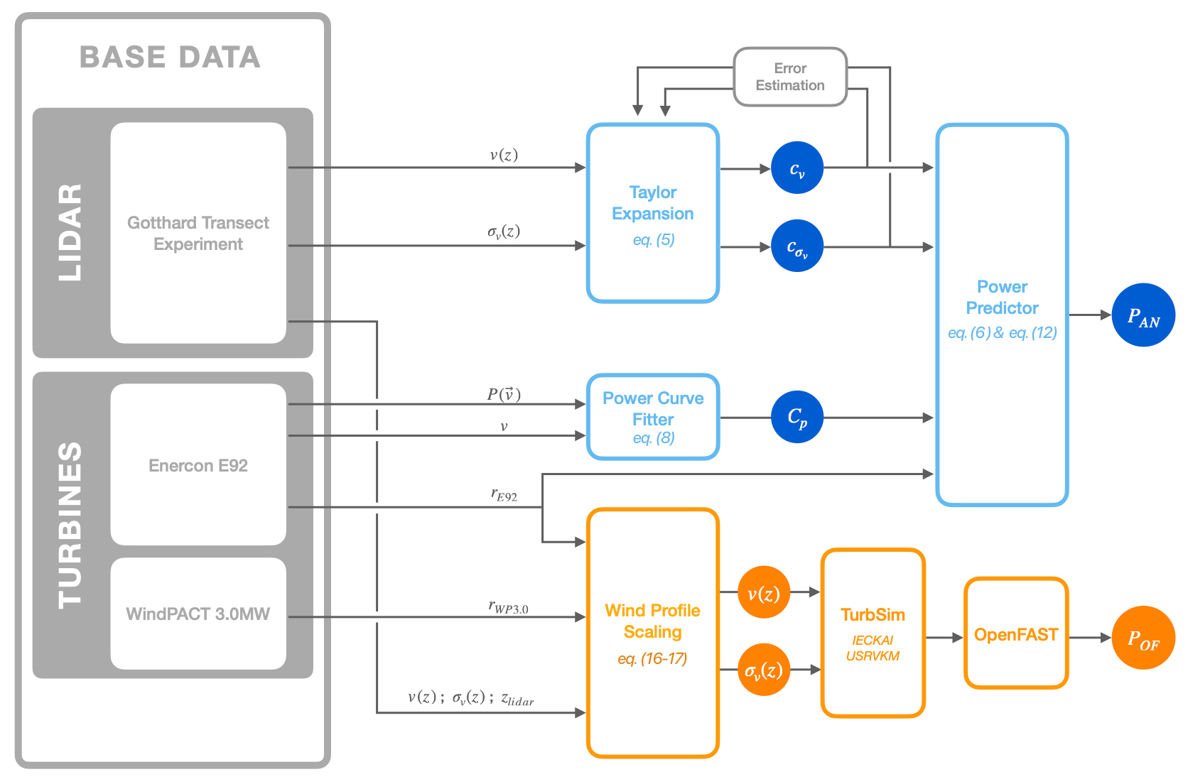
Figure 5 Schematic of the analytical and OpenFAST model workflow. The power-curve fitter returns both P_pc(U) and C_p(U); the Taylor expansion step returns coefficients for both the mean wind speed profile, c_v, and the wind speed standard-deviation profile, $c_{{\mathit{\sigma }}_v}$, when turbulence is included.

3.7 Model evaluation and wake filtering

Model predictions are evaluated against the measured 10 min power production of the five Enercon E92 turbines. Each turbine is considered separately for northerly and southerly flow, giving 10 reference cases. The primary case-wise metric is bias. Across the wake-free cases, RMSE, MAE, and the coefficient of determination are computed from the original unbinned 10 min data. Binned curves are used only for visualization and not as the basis for goodness-of-fit statistics.

Wake-contaminated profiles are treated separately. When a lidar range gate is clearly affected by a turbine wake but adjacent measurements remain representative of the undisturbed profile, the affected gates can be removed before fitting the Taylor polynomial. The analytical model is then applied to the reconstructed profile. This filtering, demonstrated in Sect. 4.3, is used only as a diagnostic test of the method's flexibility and is not included in the main wake-free model-performance statistics.

4 Results and discussion

The following results assess the performance of the newly derived analytical model against both the hub-height-based reference methods and high-fidelity OpenFAST simulations. Traditionally, the hub-height reference method relies on a single-point wind speed measurement, either taken at nacelle height or scaled from two-thirds of nacelle height, which neglects vertical wind profile variations. Our analytical model aims to overcome this limitation by explicitly accounting for vertical wind structure while remaining computationally efficient.

We begin by isolating the effects of typical features of vertical wind profiles, which includes shear, veer, and logarithmic wind profiles, as well as homogeneous turbulence intensity, through the idealized wind profile test cases. We then apply the model to 10 real-world cases applied to the 5 turbines at Gotthard Pass, distinguishing between northerly and southerly flow conditions. Finally, we highlight one case strongly affected by wake interactions and demonstrate how wake filtering can be applied to recover the undisturbed power signal and improve power prediction significantly.

4.1 Idealized wind profiles

The comparison between the power expectation from OpenFAST and the analytical model is summarized in Fig. 6. For linear shear (Fig. 6a), we find that shear effects contribute positively to the power production of the turbine in comparison to the homogeneous wind profile. The power estimated by the OpenFAST model consistently increases with shear, reflecting the cubic dependence of power on wind speed (P∝v³), where higher wind speed contributes more significantly to the overall output. Above the rated wind speed, ΔP tends to 0 as the turbine saturates at its maximum capacity, and the extra wind speed is not able to positively contribute to the power production. This is particularly well illustrated by the sudden drop of the OpenFAST curve at v=12 m s⁻¹. For the analytical model, the rated power is reached more smoothly at v=14 m s⁻¹, which can be directly attributed to the smoother curvature of the power curve as reported in Sect. 4.1.1. With increasing shear coefficient a, we see similar increases in the magnitude of ΔP for both models, and the peak values scale as expected with ∝a² as described in Eq. (15).

Concerning the differences in the two models, we can observe two elements: the apparent overestimation of the analytical model and the linear behavior of the OpenFAST curve for low velocities. The overestimation of the power difference in the analytical model is most likely caused by the several reducing factors not taken into account in the analytical model. For example, OpenFast considers the reduced efficiency of energy transfer from the wind to the turbine blade due to non-ideal angle of attack, additional shearing forces, and vibrations that will inevitably cause additional friction and reduced power production in reality.

In the case of linear veer, shown in Fig. 6b, the observations are analogous to the shear but lead to a reduction in power output instead of an increase. This reduction arises from the diminished effective wind velocity component normal to the rotor plane, which is caused by the veer angle. The shapes of both power difference curves are similarly more abrupt for the OpenFAST model due to the less refined and realistic power curve, and the analytical model reports higher differences due to a lack of dampening factors that are present in OpenFAST. As we vary the maximum veer angle α_max, the analytical model follows the expected square dependence ($\mathrm{\Delta }P\propto {\mathit{\alpha }}_{\max }^{\mathrm{2}}$) as described in Eq. (16).

The OpenFAST simulations, however, show slightly different magnitudes, with relatively larger power losses at smaller angles (α_max=5°) and smaller losses at larger angles (α_max=22.5°). This deviation is most likely due to the more detailed modeling of airflow over the blades, but it remains of secondary importance compared to the dominant quadratic dependence on α_max in determining the overall turbine power output.

The ΔP curves of homogeneous turbulence are shown in Fig. 6c. The analytical response follows directly from the curvature of the turbine power curve, as previously described by Gasser et al. (2026): turbulence increases expected power where the curve is locally convex and reduces it where the response becomes concave as rated power is approached. Increasing TI therefore increases the magnitude of the analytical turbulence contribution. The OpenFAST curve shows the same broad sign change but differs in magnitude and near-rated power. Because this stochastic OpenFAST comparison additionally depends on a prescribed turbulence spectrum and length-scale setting that are not constrained as site-specific quantities in this study, it is used here only as a qualitative aeroelastic reference; the analytical turbulence result itself does not depend on those TurbSim settings.

The final idealized profile we discuss is the logarithmic profile shown in Fig. 6d, a common profile that is used to describe the standard wind shear of the earth's surface. The curvature effects previously described for the linear shear still hold in this simulation. A noticeable observation is the relatively low impact of the logarithmic profile, with the maximum deviation from the uniform inflow amounting to only about 15 and 20 kW for the analytical and OpenFAST models, respectively. The logarithmic profile resembles the linear shear profile in shape; however the increase in wind speed is more strongly limited than the decrease. So instead of a net positive effect, as might be expected from the convexity of the power curve, it results in a small negative effect. As discussed earlier in this section, OpenFAST predicts this behavior more abruptly, while the analytical model responds more smoothly. Interestingly, in this case the analytical model predicts a smaller magnitude of change. This is likely because, in the analytical formulation, the positive contributions more strongly compensate for the negative ones, whereas OpenFAST simulations have additional sources of power loss due to friction and control dynamics of the turbine, compared to the baseline OpenFAST simulation.

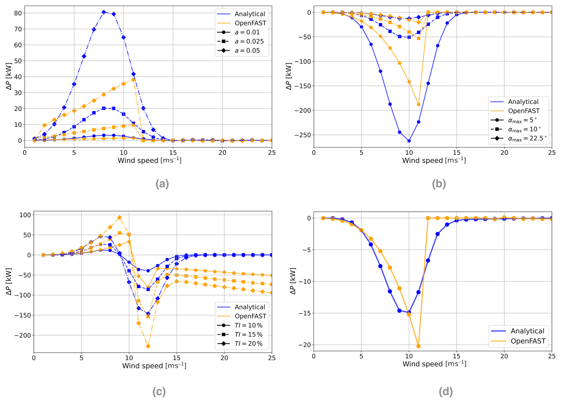
Figure 6 The difference in power production from a uniform wind profile for the four idealized vertical wind profiles. (a) Linear shear, (b) linear veer, (c) homogeneous turbulence intensity (TI), and (d) logarithmic wind profile (z₀=0.1 m).

4.1.1 Differences in power curves

The analytical model is parameterized using the power curve of the Enercon E92 2.35 MW turbines installed at the Gotthard Wind Park. The tabulated manufacturer power-curve data are fitted with the analytical expression introduced in Eq. (8), resulting in a smooth representation of P(v) and its associated power coefficient C_p(v), as shown in Fig. 7a.

The OpenFAST simulations, however, cannot be performed with the Enercon E92 directly because a complete open aeroelastic model of this turbine is not available. The numerical simulations therefore use the open-source WindPACT 3.0 MW reference turbine. This difference in turbine representation affects all comparisons between the analytical model and OpenFAST because the two turbines do not share the same power curve, controller behavior, or aerodynamic response. In particular, the WindPACT power curve exhibits features that are not representative of a modern commercial turbine power curve. Its C_p(v) reaches unrealistically high values before remaining nearly constant until rated power is reached, and the model does not include clearly defined cut-in and cut-out wind speeds. As a result, the WindPACT turbine can produce power under wind conditions for which a real turbine would normally be curtailed or shut down, which may lead to an overestimation of energy production at low and high wind speeds.

A further distinction that can be seen in Fig. 7 is that the two power curves represent different physical and methodological assumptions. The Enercon E92 power curve is based on long-term field measurements and therefore implicitly averages over a wide range of real atmospheric inflow conditions. By contrast, the WindPACT reference-turbine curve is derived for an idealized uniform inflow, where the wind speed is constant across the rotor plane. In reality, even a standard power-curve measurement includes some degree of vertical shear, veer, and turbulence and could therefore be more closely represented by a logarithmic or power-law profile than by a perfectly uniform profile. Introducing such a correction would require an additional shear parameter, such as z₀ or α, but this information is not reported for the Enercon E92 power-curve calibration. Although it would be possible to estimate such a parameter from the test-site topography, the resulting value would remain uncertain because wind shear depends strongly on atmospheric stability, surface conditions, and wind direction (Bot, 2016; Emeis, 2005).

This distinction is also relevant for the interpretation of standardized power-curve measurements. The IEC 61400-12-1:2022 standard describes power-performance testing using nacelle-mounted measurements, including nacelle-mounted lidar systems that estimate the incoming wind field upstream of the turbine (IEC, 2022; Wagner et al., 2011). Commercial nacelle-mounted lidars often scan a conical pattern, so their measurements can include information from a finite region of the rotor-swept area rather than from a single point (Letizia et al., 2023; Rettenmeier et al., 2013). The resulting nacelle wind speed signal is then calibrated against the turbine response and effectively converts a non-uniform, spatially variable inflow into a single representative wind speed value. In this sense, the manufacturer power curve already contains an implicit averaging over realistic inflow variability, whereas the OpenFAST reference curve is tied more directly to the idealized uniform-inflow assumption.

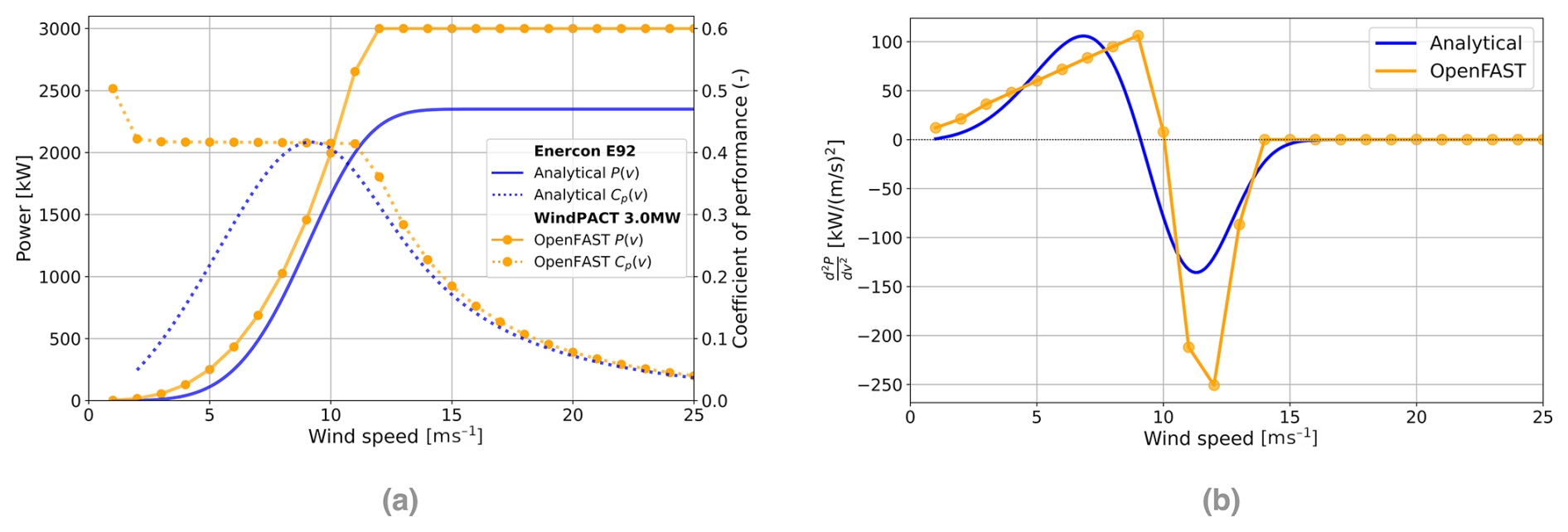
Figure 7 Comparison of the Enercon E92 2.35 MW and WindPACT 3.0 MW power curves, power coefficients, and curvature. (a) Power curves P(v) and coefficients of performance C_p(v), (b) curvature of the power curves.

The second derivative of the power curve is shown in Fig. 7b. This curvature is central to the analytical framework because it determines how wind speed variations across the rotor-swept area affect mean power production. When different parts of the rotor experience different wind speed regimes, the local curvature of P(v) controls whether these variations increase or decrease the rotor-integrated power relative to a uniform inflow. The fitted Enercon E92 curve has a smooth curvature, whereas the WindPACT curve shows a nearly linear increase followed by an abrupt transition near rated power. These differences explain several of the features observed in the idealized-profile comparisons, including the more abrupt OpenFAST response and the smoother analytical response throughout the following results.

4.2 Gotthard wind profiles

We continue by evaluating the models under real-world conditions. For this purpose we have selected 10 distinct wind events at each of the 5 turbines in the Gotthard Wind Park. Each case spans several hours and is classified by southerly or northerly flow (Table 2), which are the prevailing wind regimes for this mountain pass. For each event, we make use of the Gotthard Transect Experiment dataset (van Schaik et al., 2024), which includes 10 Doppler wind lidar deployments along the pass, providing upwind vertical wind profiles from all 5 turbines and prevailing winds.

In Fig. 8, nine of the 10 cases are shown; the case of Turbine 1 with lidar location 9 under southerly flow is omitted. The wake effects from Turbine 2 contaminating the lidar wind profiles before reaching Turbine 1 require a separate case. This special case is discussed in Sect. 4.3.

The first sub-figure (Fig. 8a) compares the predicted and observed power output, with the turbulence module enabled for both models. As observed before in Fig. 6c, the turbulence improves power output until about v=10 m s⁻¹, after which power production is decreased, reducing deviation from the true power in all cases. Compared to the turbulence-free case (Fig. 8b), this model version achieves slightly better agreement with the measured power production, which only becomes clear when considering the bias values in Table 2. Here, the analytical model clearly outperforms OpenFAST, which often overestimates power once the rated power of the turbine is reached. This behavior can also be observed from the idealized wind profiles of Fig. 6.

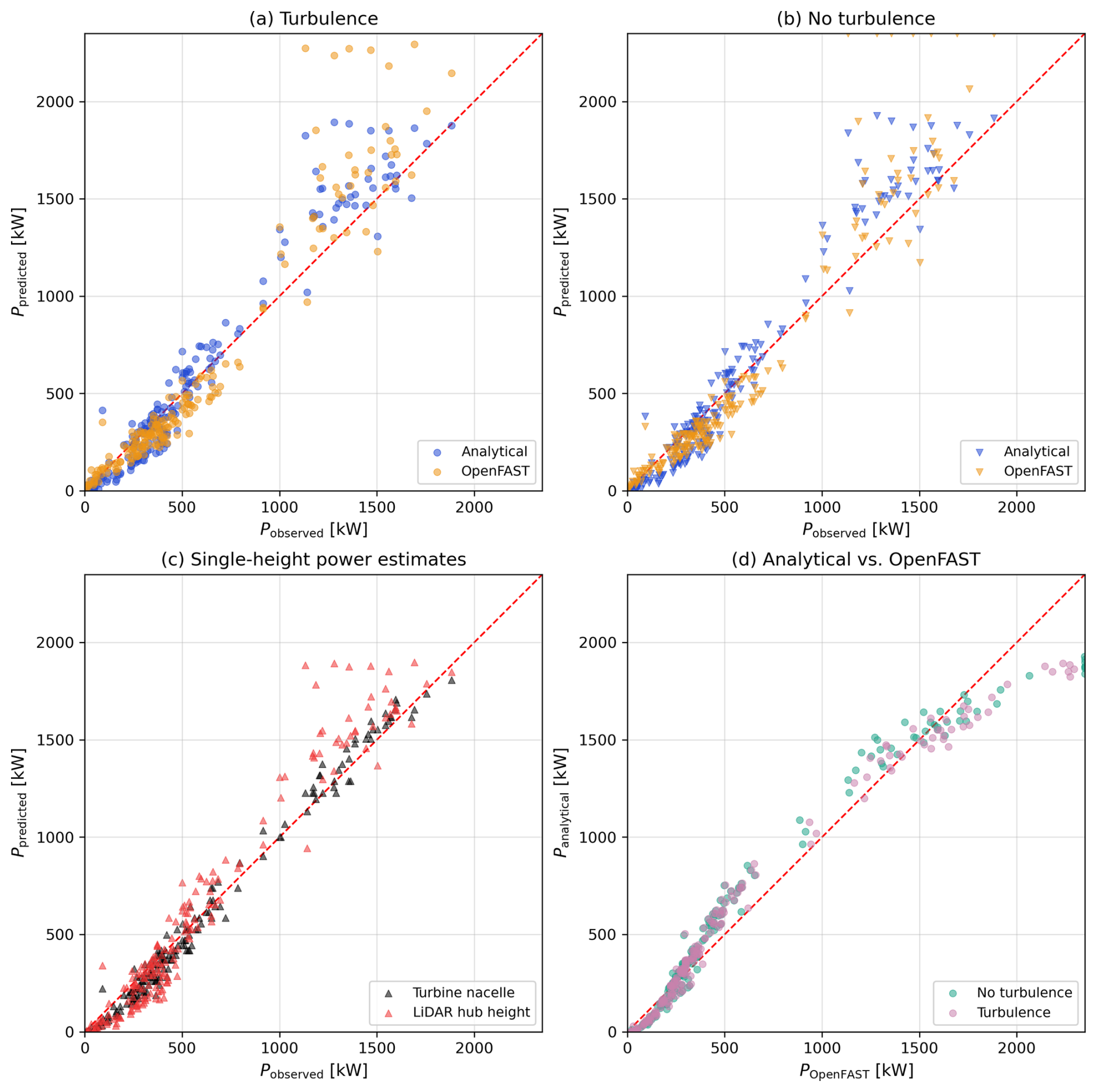
Figure 8 The differences in power production from the analytical and OpenFAST models, compared to standard approaches. Comparison of the two models (a) including turbulence and (b) excluding turbulence. (c) Standard nacelle power estimates from turbine anemometer and lidar and (d) model cross-correlations.

In Fig. 8d, the cross-correlation between the analytical and OpenFAST models is shown. A systematic pattern can be observed here. Firstly, at low wind speeds, OpenFAST generates power earlier because it lacks a defined cut-in wind speed – a known unrealistic feature of the software. This should however not affect the results in a measurable way as the selected cases do not include the trivial case where v<v_in and P=0 kW. Secondly, in the intermediate region, the analytical model produces more power due to the stronger curvature of the power curve (Fig. 7b). Finally, at higher wind speeds, OpenFAST diverges again to greater power predictions, reflecting its unrealistic post-rated behavior. Notably, the inclusion of turbulence only has a significant impact near rated power as the power curve flattens afterwards.

To connect these findings of the power prediction models to the hub-height reference methods, the third sub-figure (Fig. 8c) shows predictions based on nacelle-height wind speed alone. The trivial case is the turbine nacelle measurement itself (black), which unsurprisingly correlates well with true power since it is effectively calibrated against it. Still, small deviations indicate the importance of vertical variations in the inflow. More striking is the performance of the lidar-based nacelle-height estimations (red), which effectively serve as the hub-height-based extrapolation method. When considering the variety of the wind profiles measured by the lidar on Gotthard Pass, it becomes immediately evident that there is no single surface roughness that can be assigned to this site to perform such an extrapolation. We therefore remain at the best possible case for the hub-height reference by taking the lidar range gate closest to the elevation of the nacelle. Relative to the hub-height-based reference approach, the analytical model reports several improvements with the inclusion of the vertical wind profiles.

Table 2 Specification and error statistics of the 10 Gotthard case study sites.

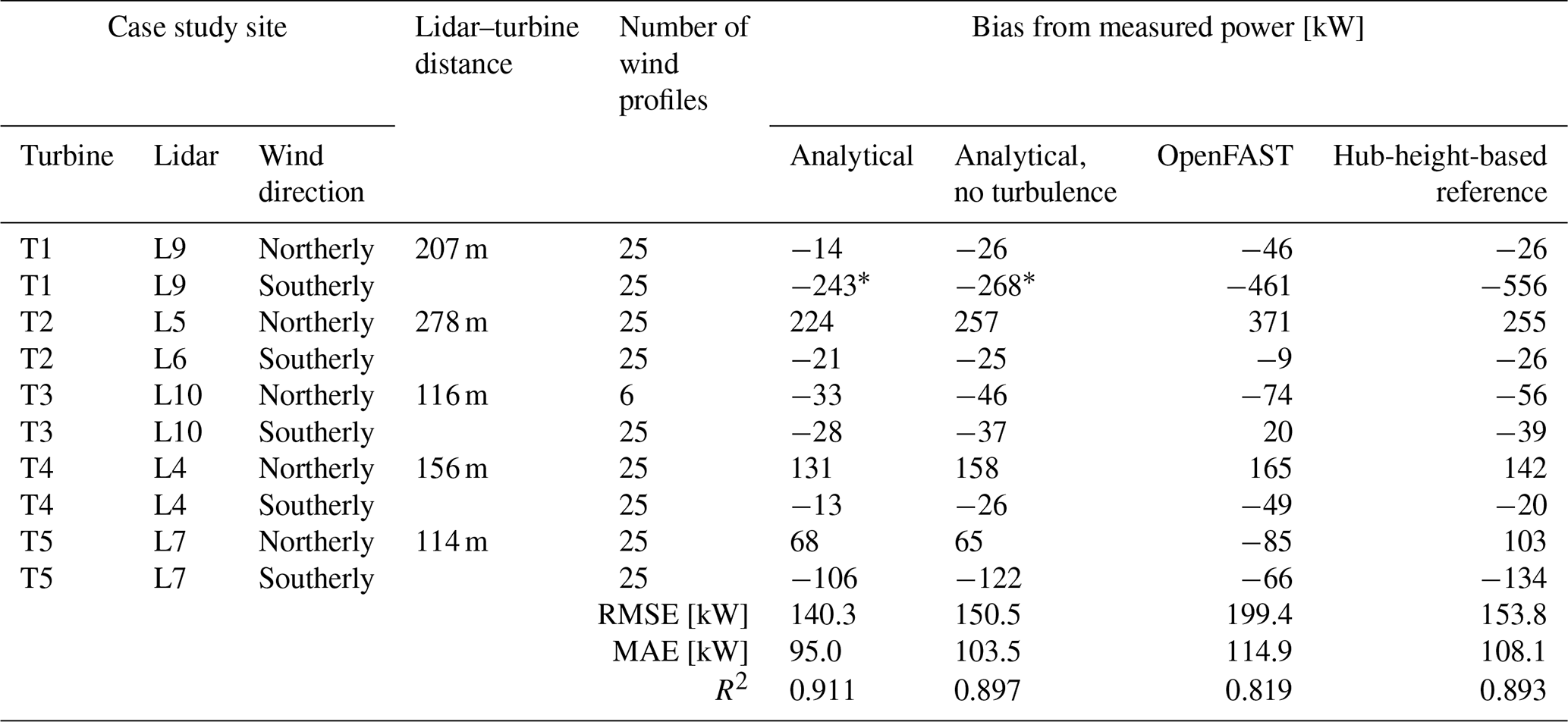
^* Corrected for wake effects.

As shown in Table 2, the reduction in absolute wind power bias relative to the hub-height-based reference approach ranges from 7.8 % to 46.4 % across the evaluated cases, with a mean reduction of 27.2±12.3 %. For each case, this reduction is calculated by subtracting the magnitude of the analytical model's bias from the magnitude of the reference approach's bias, dividing by the latter, and multiplying by 100. Positive values therefore indicate a reduction in absolute bias. The calculation uses the first and last columns of the bias section of Table 2, excluding the wake-affected T1-L9-Southerly case. The reported mean and standard deviation describe the case-wise percentage reductions. Across the evaluated wake-free cases, the analytical model also reduces RMSE by 8.8 % and MAE by 12.2 % relative to the hub-height-based reference approach. These improvements demonstrate more accurate power estimates for the investigated events; the limited selection of events does not establish a corresponding improvement in annual energy production estimates. The OpenFAST predictions, however, exhibit higher aggregate RMSE and MAE than the hub-height-based reference approach. Differences in turbine representation likely contribute to this discrepancy: the proprietary aerodynamic specifications of the Enercon E92 prevent its direct implementation in the present OpenFAST simulations. Instead, the open-source WindPACT 3.0 MW reference turbine was used, and its power output was scaled by the rated-power ratio. This scaling does not account for differences in power-curve shape or aerodynamic response, thereby limiting the comparability of the results.

For the turbulent Gotthard OpenFAST cases, USRVKM is retained specifically because it preserves the measured height-dependent σ_v(z) profile. As discussed in Sect. 3.5, the associated example length-scale settings are not interpreted physically. A representative rerun with the IEC Kaimal NTM for the highest-turbulence case produced essentially the same case-wise bias and did not improve the scatter. The turbulent OpenFAST results are therefore treated as a secondary numerical consistency check rather than as a site-specific turbulence-spectrum validation.

Overall, the results show that while nacelle-height extrapolation can provide reasonable fits, the analytical model generalizes significantly better for complex-terrain site assessments. Including turbulence further sharpens its predictive skill, particularly at high wind speeds, while retaining negligible computational cost compared to OpenFAST.

4.3 Wake filtering

In Fig. 9a, the original lidar wind measurements from lidar location 9 for southerly wind conditions, relative to Turbine 1, are shown in orange, together with a subset of points selected outside the wake-contaminated region. From the analysis of wake direction and extent, this case was identified as the only instance where either the lidar or the turbine is affected by a wake. Specifically, for Turbine 1 and lidar location 9 under southerly wind conditions, the wake from Turbine 2 intersects the lidar beam but consistently bypasses Turbine 1. This becomes evident when considering the turbine position angle of Turbine 2: extending a line downstream on the lee side of the turbine while accounting for the swept area of the rotor shows that the wake passes over lidar location 9 but does not intersect Turbine 1. As a result, the lidar profile misrepresents the true inflow conditions of the turbine.

The error bars of both the orange and green profiles, as well as the shaded blue region, represent the standard deviation of the wind speed during the 10 min time window, in which complete wind profiles are measured every 5 s. After wake filtering, the resulting profile (blue) behaves much more consistently as if no wake were present, which is also observed by the reduced turbulence intensity, also interpolated by the Taylor expansion.

The effect on power predictions due to the filtering of the wake is shown in Fig. 9b. The unfiltered case, with analytical and OpenFAST predictions in blue and orange, respectively, substantially underestimates the measured turbine power. After applying the wake filter, the analytical results align much more closely with the actual turbine production. Quantitatively, the RMSE decreases from 515.8 to 242.9 kW, which is a reduction of 53 %, while the bias is reduced by 58 % to −215.3 kW. The only trade-off is a slight decrease in correlation, from 0.55 to 0.50, indicating that the effectiveness of the wake correction varies between individual profiles. This is to be expected as the procedure simply removes a standard range of wind measurements where the wake is expected based on the height of the swept area of Turbine 2 with respect to the elevation of the lidar. In some cases, particularly when the wind field contains a vertical component, wake remnants may still contaminate the higher points, or the correction may overcompensate, as visible in one outlier above the 1:1 line.

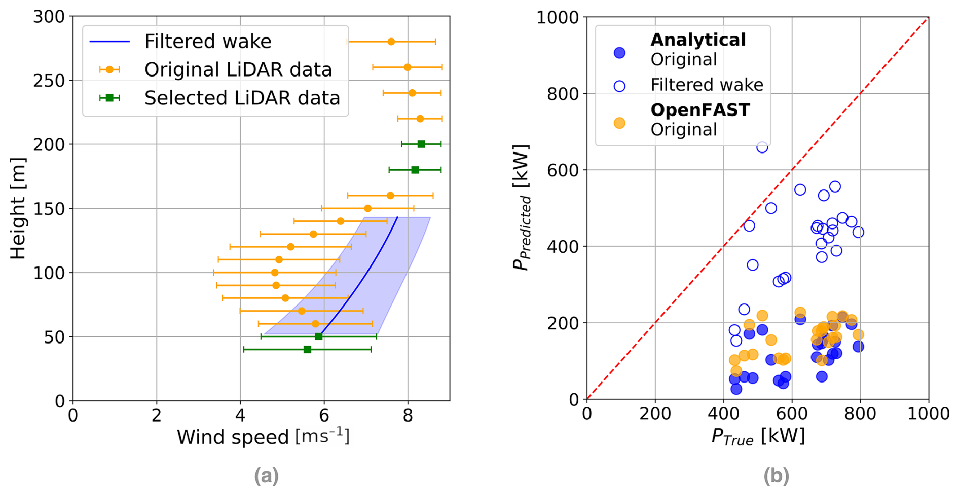
Figure 9 Wake filtering of lidar location 9 with Turbine 1 under southerly winds: (a) wind profile and (b) power production comparison.

Despite these limitations, the approach works remarkably well and highlights a key advantage of the analytical model: it can be applied flexibly to almost any kind of input data. Whether only two measurement levels are available or a densely resolved lidar profile, the Taylor expansion method adapts naturally. This stands in stark contrast to the OpenFAST method, which cannot directly accommodate such filtering. Importantly, the method is also turbine-independent: even before a specific turbine type is selected, a single lidar deployment can provide accurate wind energy assessments for any size turbine. Furthermore, wake-filtered profiles can be particularly valuable in cases such as wind farm expansions, where wake contamination is unavoidable, yet filtering offers a practical way to recover representative inflow profiles such as in off-shore applications where one can expect the unaffected wind profile to be similar within a few kilometers from the lidar site.

4.4 Robustness and sensitivity tests

In addition to the core results, several supplementary tests were conducted to evaluate the robustness of the analytical model. First, the shaft tilt was tested. In the main numerical simulations, the shaft tilt is set to 0° to remain consistent with the analytical formulation. A more realistic value of 5°, as reported in the Enercon E92 technical specifications, introduces a small bias of approximately 8 kW for the 2.35 MW turbine. However, since the wind profile is based on a lidar measurement located roughly 100 m from the turbine, any slight decrease in horizontal inflow or inclusion of vertical wind components caused by shaft tilt would not necessarily improve the accuracy of the comparison. The simpler 0° configuration is therefore retained, as it is more directly comparable to the idealized wind profile experiments.

Secondly, the sensitivity to air density was investigated using OpenFAST simulations across a range of values representative of wind parks at different elevations. The analytical model remains well behaved across the full range, with no need to adjust the shape of the C_p(v) curve. This confirms that the formulation can be transferred to sites at different elevations, provided that the air-density dependence of available wind power is treated consistently.

Thirdly, we tested the impact of using alternative turbine power curves. When replacing the Enercon E92 curve with the WindPACT 3.0 MW reference-turbine curve, the agreement between the analytical model and OpenFAST becomes closer, although this improvement is primarily due to a degradation of the analytical model rather than an enhancement of OpenFAST. This illustrates that the framework can be applied to arbitrary power curves, as the analytical approximation in Eq. (8) is flexible and well behaved.

Finally, we assessed the impact of temporal averaging on estimates of $\stackrel{\mathrm{‾}}{v^{\mathrm{3}}}$ by aggregating the 1 s lidar wind speed data over a range of averaging intervals: 1, 2, 5, 10, 20, and 30 min and 1 h. Changing the averaging window slightly modifies the resulting wind profiles, which in turn affects the analytically derived power production. These differences remain relatively small, on the order of 4 % (on the order of 3 kW for the 3 MW turbine at TI=15 %). While this effect is not explored further, it is noted as a minor source of uncertainty. In line with standard wind energy practice, 10 min averages are adopted throughout this study.

Together, these tests demonstrate that the analytical model is robust to variations in shaft tilt, air density, turbine power curve, and temporal averaging. The separate choice of turbulence spectrum used to generate the secondary turbulent OpenFAST comparison is discussed in Sect. 3.5 and is not used to draw conclusions about Gotthard turbulence physics.

5 Conclusions

In this study, we introduced and validated a new analytical framework for predicting wind turbine power production that explicitly accounts for vertical wind profile variability through an integral formulation. By combining Taylor expansions of the inflow with an analytical representation of the turbine power curve, the model provides a clearly improved alternative to the hub-height-based reference for wind energy assessment based on a single nacelle-height wind measurement. Furthermore, it provides a flexible alternative to costly numerical simulation of wind turbine aerodynamics.

The results show that the primary discrepancies between the analytical model and OpenFAST can be attributed to differences in the turbine power curves. While the analytical model was configured for the Enercon E-92 turbine, reflecting the real-world lidar measurements at Gotthard Pass, OpenFAST required the use of the WindPACT 3.0 MW reference turbine. The unusual C_p(v) curve of the latter, including the absence of realistic cut-in and cut-out wind speeds, amplified differences in the response to vertical wind profile variations. This effect is best represented by considering the curvature ($\frac{d^{\mathrm{2}}P}{d{v}^{\mathrm{2}}}$) of the power curve, which confirms the mechanism and provides an explanation for the observed discrepancies in the predicted power of the turbines.

When applying the analytical model to idealized wind profiles, such as linear shear, linear veer, logarithmic wind profiles, and homogeneous turbulence intensities, we demonstrated that the analytical formulation produces smoother and more physically consistent power predictions compared to OpenFAST. These differences are likely driven by the different power curves.

This same effect is also visible in the real Gotthard lidar profiles, which provided a direct validation against real-world inflow conditions. The vertical wind profiles at this alpine site are strongly shaped by shear, veer, and turbulence and represent a complex but highly relevant test case for wind energy production. Compared to OpenFAST, the analytical model showed smoother and more consistent responses to these profiles, reflecting the more regular curvature of the Enercon E-92 power curve used in its formulation. Across the evaluated wake-free cases, the analytical model achieved a coefficient of determination of R²=0.911 and a mean reduction in absolute case-wise bias of 27.2±12.3 % relative to the hub-height-based reference approach. These results demonstrate improved power estimates for the investigated events.

The wake filtering analysis further illustrated the strength of the analytical approach by means of its flexibility: by excluding the portion of the lidar profile affected by a turbine wake, the analytical model predictions were brought significantly closer to the measured power, reducing the RMSE and bias by more than 50 %, significantly closer to the typical skill of the other cases, although the slight decrease in correlation suggests that this method does not work as effectively on the wind profile due to leaking over wake effects. Further work should consult the plethora of literature available on wake detection, which will likely be the remedy to this rather straightforward problem, which is outside of the scope of this work.

Further robustness and sensitivity tests confirmed that the analytical framework performs consistently across a range of air densities representative of all elevations and that the method can be applied to arbitrary power curves thanks to the analytical approximation of Eq. (8). The OpenFAST turbulence-spectrum choice is treated only as a secondary numerical consideration and is not used to infer site-specific turbulence length scales. We also tested the sensitivity to the 10 min averaging window used throughout wind energy practice and found a small additional uncertainty of up to approximately 4 % in the analytical power prediction. This effect is minor relative to the main model differences considered here.

In summary, the analytical model developed here applies a simple physical interpretation of vertical variations in the wind in a computationally efficient and highly flexible tool for assessing turbine power production under vertically varying wind conditions. It captures the essential mechanisms behind power output variations; explains discrepancies with simulation-based models through power-curve curvature; and can be robustly applied across sites, turbines, and measurement configurations. Beyond its application in the Swiss Alps with the Gotthard Pass case study, the model offers a new pathway to bridge measurements that we think should be considered as an amendment to today's wind energy assessment standards, as it is low-impact due to our open-source code for the tool and the trend of using lidar in site selection for wind parks, which already include this additional information of vertical wind profiles. We particularly want to highlight the value in the practicality of use in the majority of cases where wind turbine aerodynamic specifications are proprietary, something that more sophisticated simulations and other state-of-the-art tools require, which is completely avoidable by this method.

Appendix A: Analytical power equation derivation

From Taylor series theory, a continuous function such as the wind speed profile can be approximated by a polynomial:

$$\begin{array}{}\text{(A1)}& v\left(z\right)=\sum _{i=\mathrm{0}}^N{c}_i{z}^i.\end{array}$$

The standard turbine power equation is

$$\begin{array}{}\text{(A2)}& P\left(z\right)={\displaystyle \frac{\mathrm{1}}{\mathrm{2}}}{C}_{\mathrm{p}}\left(v\right)\mathit{\rho }Av(z{)}^{\mathrm{3}}.\end{array}$$

We integrate over the circular swept area by converting the surface integral to a 1D integral in height:

$$\begin{array}{}\text{(A3)}& P={\displaystyle \frac{\mathrm{1}}{\mathrm{2}}}{C}_{\mathrm{p}}\left(v\right)\mathit{\rho }\underset{-R}{\overset{R}{\int }}\mathrm{2}\sqrt{R^{\mathrm{2}}-z^{\mathrm{2}}}v(z{)}^{\mathrm{3}}\text{d}z.\end{array}$$

To integrate over the height z, we must define the cube of the wind speed that is parallel to the normal vector of the swept area:

$$\begin{array}{}\text{(A4)}& \begin{array}{rl}{\left(v\left(z\right)\right)}^{\mathrm{3}}& =\sum _{i,j,k=\mathrm{0}}^N{c}_i{c}_j{c}_k{z}^{i+j+k}\\ & =\sum _{i=\mathrm{0}}^N\left(c_i\sum _{j=\mathrm{0}}^N\left(c_j\sum _{k=\mathrm{0}}^N\left(c_k{z}^{i+j+k}\right)\right)\right)\end{array}.\end{array}$$

We solve this analytically by the following substitution:

$$\begin{array}{}\text{(A5)}& z=R\sin \left(u\right),u=\arcsin \left({\displaystyle \frac{z}{R}}\right),\text{d}z=R\cos \left(u\right)\text{d}u,\end{array}$$

such that the power equation becomes

$$\begin{array}{}\text{(A6)}& \begin{array}{rl}P(v,u)& ={\displaystyle \frac{\mathrm{1}}{\mathrm{2}}}{C}_{\mathrm{p}}\left(v\right)\mathit{\rho }\underset{\frac{-\mathit{\pi }}{\mathrm{2}}}{\overset{\frac{\mathit{\pi }}{\mathrm{2}}}{\int }}\mathrm{2}R\cos \left(u\right)\sqrt{R^{\mathrm{2}}-R^{\mathrm{2}}{\sin }^{\mathrm{2}}\left(u\right)}\\ & \times \sum _{i,j,k=\mathrm{0}}^N{c}_i{c}_j{c}_k{R}^{i+j+k}{\sin }^{i+j+k}\left(u\right)\text{d}u.\end{array}\end{array}$$

This is simplified by removing the factor 2 out of the integral and by rearranging the square root:

$$\begin{array}{}\text{(A7)}& \begin{array}{rl}P(v,u)& =C_{\mathrm{p}}\left(v\right)\mathit{\rho }\underset{\frac{-\mathit{\pi }}{\mathrm{2}}}{\overset{\frac{\mathit{\pi }}{\mathrm{2}}}{\int }}R\cos \left(u\right)\sqrt{R^{\mathrm{2}}(\mathrm{1}-{\sin }^{\mathrm{2}}(u\left)\right)}\\ & \times \sum _{i,j,k=\mathrm{0}}^N{c}_i{c}_j{c}_k{R}^{i+j+k}{\sin }^{i+j+k}\left(u\right)\text{d}u.\end{array}\end{array}$$

The square root can be resolved by a trigonometric substitution to find

$$\begin{array}{}\text{(A8)}& \begin{array}{rl}P(v,u)& =C_{\mathrm{p}}\left(v\right)\mathit{\rho }\underset{\frac{-\mathit{\pi }}{\mathrm{2}}}{\overset{\frac{\mathit{\pi }}{\mathrm{2}}}{\int }}{R}^{\mathrm{2}}{\cos }^{\mathrm{2}}\left(u\right)\\ & \times \sum _{i,j,k=\mathrm{0}}^N{c}_i{c}_j{c}_k{R}^{i+j+k}{\sin }^{i+j+k}\left(u\right)\text{d}u.\end{array}\end{array}$$

We can move the triple summation, including several constants, out of the integral to simplify the integral to a purely trigonometric problem:

$$\begin{array}{}\text{(A9)}& \begin{array}{rl}P(v,u)& =C_{\mathrm{p}}\left(v\right)\mathit{\rho }{R}^{\mathrm{2}}\sum _{i,j,k=\mathrm{0}}^N{c}_i{c}_j{c}_k{R}^{i+j+k}\\ & \times \underset{\frac{-\mathit{\pi }}{\mathrm{2}}}{\overset{\frac{\mathit{\pi }}{\mathrm{2}}}{\int }}{\cos }^{\mathrm{2}}\left(u\right){\sin }^{i+j+k}\left(u\right)\text{d}u.\end{array}\end{array}$$

We now focus on the integral only, by defining it as Q_m:

$$\begin{array}{}\text{(A10)}& P(v,u)=C_{\mathrm{p}}\left(v\right)\mathit{\rho }{R}^{\mathrm{2}}\sum _{i,j,k=\mathrm{0}}^N{c}_i{c}_j{c}_k{R}^{i+j+k}{Q}_m\left(u\right),\end{array}$$

where the substitution Q(z) also replaces $i+j+k$ by a new integer m,

$$\begin{array}{}\text{(A11)}& Q_m\left(u\right)=\underset{\frac{-\mathit{\pi }}{\mathrm{2}}}{\overset{\frac{\mathit{\pi }}{\mathrm{2}}}{\int }}{\cos }^{\mathrm{2}}\left(u\right){\sin }^m\left(u\right)\text{d}u,m=i+j+k.\end{array}$$

For odd values of m, the integrand cos ²(u)sin ^m(u) is an odd function, and the integral over the symmetric interval $[-\mathit{\pi }/\mathrm{2},\mathit{\pi }/\mathrm{2}]$ evaluates to 0:

$$\begin{array}{}\text{(A12)}& Q_m\left(u\right)=\mathrm{0},\text{if }m\text{ is odd}.\end{array}$$

For even values of m, let m=2s, where s is an integer. The integrand cos ²(u)sin ^2s(u) is an even function, and by symmetry, the integral can be simplified by doubling the range from $[\mathrm{0},\mathit{\pi }/\mathrm{2}]$:

$$\begin{array}{}\text{(A13)}& Q_m\left(u\right)=\mathrm{2}\underset{\mathrm{0}}{\overset{\frac{\mathit{\pi }}{\mathrm{2}}}{\int }}{\cos }^{\mathrm{2}}\left(u\right){\sin }^{\mathrm{2}s}\left(u\right)\text{d}u,\text{if }m=\mathrm{2}s.\end{array}$$

We once again apply the trigonometric identity to eliminate the cosine from the integrand.

$$\begin{array}{}\text{(A14)}& Q_m\left(u\right)=\mathrm{2}\underset{\mathrm{0}}{\overset{\frac{\mathit{\pi }}{\mathrm{2}}}{\int }}\left(\mathrm{1}-{\sin }^{\mathrm{2}}\left(u\right)\right){\sin }^{\mathrm{2}s}\left(u\right)\text{d}u,\text{if }m=\mathrm{2}s\end{array}$$

Using $\mathrm{1}-{\sin }^{\mathrm{2}}\left(u\right)={\cos }^{\mathrm{2}}\left(u\right)$, this becomes

$$\begin{array}{}\text{(A15)}& Q_m\left(u\right)=\mathrm{2}\underset{\mathrm{0}}{\overset{\frac{\mathit{\pi }}{\mathrm{2}}}{\int }}{\sin }^{\mathrm{2}s}\left(u\right){\cos }^{\mathrm{2}}\left(u\right)\mathrm{d}u.\end{array}$$

This integral directly corresponds to the Beta function, yielding

$$\begin{array}{}\text{(A16)}& Q_m\left(u\right)=B\left(s+{\displaystyle \frac{\mathrm{1}}{\mathrm{2}}},{\displaystyle \frac{\mathrm{3}}{\mathrm{2}}}\right),\end{array}$$

where B(x,y) is the Beta function, defined as $B(x,y)=\frac{\mathrm{\Gamma }\left(x\right)\mathrm{\Gamma }\left(y\right)}{\mathrm{\Gamma }(x+y)}$, such that Q_m(u), for even values of m=2s, is given by

$$\begin{array}{}\text{(A17)}& Q_m\left(u\right)=\sqrt{\mathit{\pi }}\left({\displaystyle \frac{\mathrm{\Gamma }\left(s+\frac{\mathrm{1}}{\mathrm{2}}\right)}{\mathrm{\Gamma }(s+\mathrm{1})}}-{\displaystyle \frac{\mathrm{\Gamma }\left(s+\frac{\mathrm{3}}{\mathrm{2}}\right)}{\mathrm{\Gamma }(s+\mathrm{2})}}\right),\end{array}$$

and the turbine power equation is given by

$$\begin{array}{}\text{(A18)}& \begin{array}{rl}P\left(v\right)& =C_{\mathrm{p}}\left(v\right)\mathit{\rho }{R}^{\mathrm{2}}\sum _{i,j,k=\mathrm{0}}^N{c}_i{c}_j{c}_k{R}^m\sqrt{\mathit{\pi }}\\ & \times \left({\displaystyle \frac{\mathrm{\Gamma }\left(s+\frac{\mathrm{1}}{\mathrm{2}}\right)}{\mathrm{\Gamma }(s+\mathrm{1})}}-{\displaystyle \frac{\mathrm{\Gamma }\left(s+\frac{\mathrm{3}}{\mathrm{2}}\right)}{\mathrm{\Gamma }(s+\mathrm{2})}}\right),\\ & m=\mathrm{2}s=i+j+k|m\text{ is even},\end{array}\end{array}$$

which is only a function of wind speed v again.

The Gamma function Γ(x) is defined by

$$\begin{array}{}\text{(A19)}& \mathrm{\Gamma }\left(x\right)=\underset{\mathrm{0}}{\overset{\mathrm{\infty }}{\int }}{t}^{z-\mathrm{1}}{e}^{-t}\text{d}t.\end{array}$$

For positive integers, where $x=s=m/\mathrm{2}=(i+j+k)/\mathrm{2}$ (with m the sum of the three positive integers), the Gamma function simplifies as

$$\begin{array}{}\text{(A20)}& \mathrm{\Gamma }\left(m\right)=(m-\mathrm{1})\mathrm{!}\end{array}$$

To evaluate the Gamma function at half-integer values, consider $z=m+\frac{\mathrm{1}}{\mathrm{2}}$, where m is a non-negative integer. The key idea comes from using the recursive property of the Gamma function and its relationship with the factorial for half-integer arguments.

Using the reflection formula and the recurrence relation

$$\begin{array}{}\text{(A21)}& \mathrm{\Gamma }\left({\displaystyle \frac{\mathrm{1}}{\mathrm{2}}}\right)=\sqrt{\mathit{\pi }}\end{array}$$

and for higher half-integer values, you apply the recurrence relation $\mathrm{\Gamma }(z+\mathrm{1})=z\mathrm{\Gamma }\left(z\right)$ repeatedly. The general result for half-integer values of $\mathrm{\Gamma }\left(n+\frac{\mathrm{1}}{\mathrm{2}}\right)$ (where n is a non-negative integer) is

$$\begin{array}{}\text{(A22)}& \mathrm{\Gamma }\left(s+{\displaystyle \frac{\mathrm{1}}{\mathrm{2}}}\right)={\displaystyle \frac{\left(\mathrm{2}s\right)\mathrm{!}}{{\mathrm{4}}^{s}s\mathrm{!}}}\sqrt{\mathit{\pi }}.\end{array}$$

Thus, the Gamma function evaluated at half-integers $s+\frac{\mathrm{1}}{\mathrm{2}}$ is a product of a factorial expression, $\sqrt{\mathit{\pi }}$, and powers of 4.

Finally we can replace the full integer Gamma functions:

$$\begin{array}{}\text{(A23)}& \begin{array}{rl}P\left(v\right)& =C_{\mathrm{p}}\left(v\right)\mathit{\rho }\sqrt{\mathit{\pi }}{R}^{\mathrm{2}}\sum _{i,j,k=\mathrm{0}}^N{c}_i{c}_j{c}_k{R}^m\\ & \times \left({\displaystyle \frac{\mathrm{\Gamma }(s+\frac{\mathrm{1}}{\mathrm{2}})}{s\mathrm{!}}}-{\displaystyle \frac{\mathrm{\Gamma }(s+\frac{\mathrm{3}}{\mathrm{2}})}{(s+\mathrm{1})\mathrm{!}}}\right),\\ & m=\mathrm{2}s=i+j+k|m\text{ is even}.\end{array}\end{array}$$

We apply the recurrence relation to the $\mathrm{\Gamma }(s+\frac{\mathrm{3}}{\mathrm{2}})$:

$$\begin{array}{}\text{(A24)}& \begin{array}{rl}P\left(v\right)& =C_{\mathrm{p}}\left(v\right)\mathit{\rho }\sqrt{\mathit{\pi }}{R}^{\mathrm{2}}\sum _{i,j,k=\mathrm{0}}^N{c}_i{c}_j{c}_k{R}^m\\ & \times \left({\displaystyle \frac{\mathrm{\Gamma }(s+\frac{\mathrm{1}}{\mathrm{2}})}{s\mathrm{!}}}-{\displaystyle \frac{\left(s+\frac{\mathrm{1}}{\mathrm{2}}\right)\mathrm{\Gamma }(s+\frac{\mathrm{1}}{\mathrm{2}})}{(s+\mathrm{1})\mathrm{!}}}\right),\\ & m=\mathrm{2}s=i+j+k|m\text{ is even}.\end{array}\end{array}$$

We rearrange to a single Gamma function:

$$\begin{array}{}\text{(A25)}& \begin{array}{rl}P\left(v\right)& =C_{\mathrm{p}}\left(v\right)\mathit{\rho }\sqrt{\mathit{\pi }}{R}^{\mathrm{2}}\sum _{i,j,k=\mathrm{0}}^N{c}_i{c}_j{c}_k{R}^m\\ & \times \left({\displaystyle \frac{(s+\mathrm{1})\mathrm{!}-s\mathrm{!}(s+\frac{\mathrm{1}}{\mathrm{2}})}{s\mathrm{!}(s+\mathrm{1})\mathrm{!}}}\mathrm{\Gamma }\left(s+{\displaystyle \frac{\mathrm{1}}{\mathrm{2}}}\right)\right),\\ & m=\mathrm{2}s=i+j+k|m\text{ is even}.\end{array}\end{array}$$

We reduce the (s+1)! to s!(s+1):

$$\begin{array}{}\text{(A26)}& \begin{array}{rl}P\left(v\right)& =C_{\mathrm{p}}\left(v\right)\mathit{\rho }\sqrt{\mathit{\pi }}{R}^{\mathrm{2}}\sum _{i,j,k=\mathrm{0}}^N{c}_i{c}_j{c}_k{R}^m\\ & \times \left({\displaystyle \frac{s\mathrm{!}(s+\mathrm{1})-s\mathrm{!}(s+\frac{\mathrm{1}}{\mathrm{2}})}{s\mathrm{!}(s+\mathrm{1})\mathrm{!}}}\mathrm{\Gamma }\left(s+{\displaystyle \frac{\mathrm{1}}{\mathrm{2}}}\right)\right),\\ & m=\mathrm{2}s=i+j+k|m\text{ is even},\end{array}\end{array}$$

which cancels out the s!:

$$\begin{array}{}\text{(A27)}& \begin{array}{rl}P\left(v\right)& =C_{\mathrm{p}}\left(v\right)\mathit{\rho }\sqrt{\mathit{\pi }}{R}^{\mathrm{2}}\sum _{i,j,k=\mathrm{0}}^N{c}_i{c}_j{c}_k{R}^m\\ & \times \left({\displaystyle \frac{\mathrm{1}}{\mathrm{2}}}{\displaystyle \frac{\mathrm{1}}{(s+\mathrm{1})\mathrm{!}}}\mathrm{\Gamma }\left(s+{\displaystyle \frac{\mathrm{1}}{\mathrm{2}}}\right)\right),\\ & m=\mathrm{2}s=i+j+k|m\text{ is even}.\end{array}\end{array}$$

We finally use the general result for half-integer values of the Gamma function to find

$$\begin{array}{}\text{(A28)}& \begin{array}{rl}P\left(v\right)& =C_{\mathrm{p}}\left(v\right)\mathit{\rho }\mathit{\pi }{R}^{\mathrm{2}}\sum _{i,j,k=\mathrm{0}}^N{c}_i{c}_j{c}_k{R}^m{\displaystyle \frac{\mathrm{1}}{\mathrm{2}}}{\displaystyle \frac{\mathrm{1}}{(s+\mathrm{1})\mathrm{!}}}{\displaystyle \frac{\left(\mathrm{2}s\right)\mathrm{!}}{{\mathrm{4}}^{s}s\mathrm{!}}},\\ & m=\mathrm{2}s=i+j+k|m\text{ is even},\end{array}\end{array}$$

where the $\sqrt{\mathit{\pi }}$ reunites with the other $\sqrt{\mathit{\pi }}$ to arrange A=πR², which obviously refers to the swept area of the blade A. We also replace s with $m/\mathrm{2}$:

$$\begin{array}{}\text{(A29)}& \begin{array}{rl}P\left(v\right)& =C_{\mathrm{p}}\left(v\right)\mathit{\rho }\mathit{\pi }{R}^{\mathrm{2}}\sum _{i,j,k=\mathrm{0}}^N{c}_i{c}_j{c}_k{R}^m{\displaystyle \frac{\mathrm{1}}{\mathrm{2}}}{\displaystyle \frac{\mathrm{1}}{(\frac{m}{\mathrm{2}}+\mathrm{1})\mathrm{!}}}{\displaystyle \frac{m\mathrm{!}}{{\mathrm{2}}^m\frac{m}{\mathrm{2}}\mathrm{!}}},\\ & m=i+j+k|m\text{ is even}.\end{array}\end{array}$$

Some final mathematical bookkeeping where the half is moved to the front and πR² is combined to reflect the regular expression of the power equation, as well as by rearranging the factorials and exponents of 2, results in

$$\begin{array}{}\text{(A30)}& \begin{array}{rl}P\left(v\right)& ={\displaystyle \frac{\mathrm{1}}{\mathrm{2}}}{C}_{\mathrm{p}}\left(v\right)\mathit{\rho }A\sum _{i,j,k=\mathrm{0}}^N{c}_i{c}_j{c}_k{R}^m{\displaystyle \frac{m\mathrm{!}}{{\mathrm{2}}^m\left(\frac{m}{\mathrm{2}}\mathrm{!}{)}^{\mathrm{2}}\right(\frac{m}{\mathrm{2}}+\mathrm{1})}},\\ & m=i+j+k|m\text{ is even},\end{array}\end{array}$$

which brings us back to the familiar structure of the turbine power Eq. (2).

This demonstrates that a general analytical solution exists for the turbine power output for any continuous inflow wind profile (v(h)).

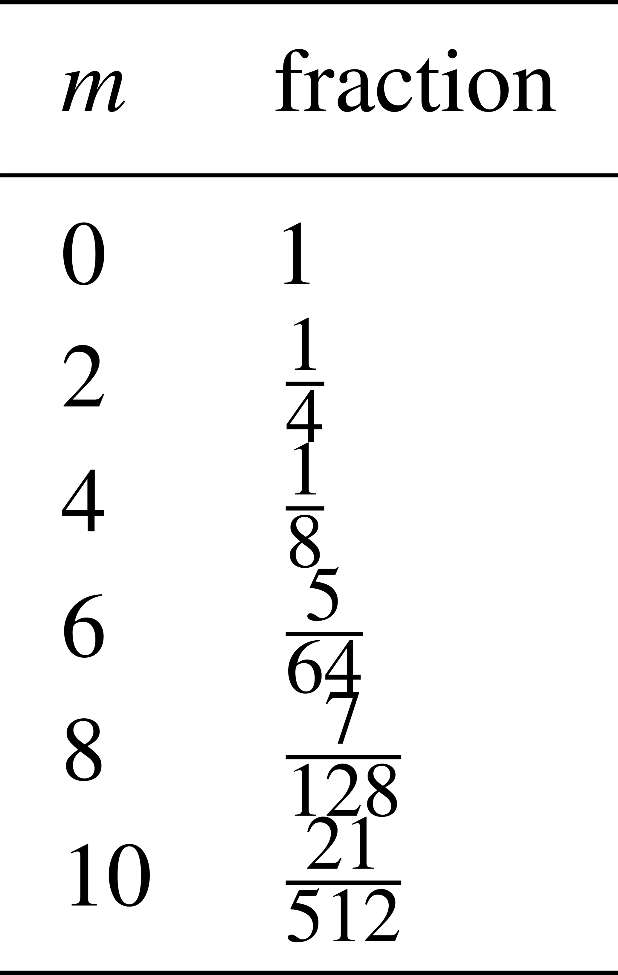
This large fraction of factorials is separated for readability and defined as K_m. It only has to be calculated for even values of m and can be found for m≤10 in Table A1:

$$\begin{array}{}\text{(A31)}& K_m={\displaystyle \frac{m\mathrm{!}}{{\mathrm{2}}^m{\left(\frac{m}{\mathrm{2}}\mathrm{!}\right)}^{\mathrm{2}}\left(\frac{m}{\mathrm{2}}+\mathrm{1}\right)}},m=i+j+k|m\text{ is even}.\end{array}$$

Table A1 Look-up table for values of m for the large factorial fraction K_m.

A1 Verification: units

As verification of this derivation, we can check the units of this equation:

$$\begin{array}{}\text{(A32)}& {\displaystyle }P& {\displaystyle }\to \left[\mathrm{W}=\mathrm{N}\mathrm{m}{\mathrm{s}}^{-\mathrm{1}}=\mathrm{kg}{\mathrm{m}}^{\mathrm{2}}{\mathrm{s}}^{-\mathrm{3}}\right],\text{(A33)}& {\displaystyle }{C}_{\mathrm{p}}& {\displaystyle }\to \left[\mathrm{1}\right],\text{(A34)}& {\displaystyle }\mathit{\rho }& {\displaystyle }\to \left[\mathrm{kg}{\mathrm{m}}^{-\mathrm{3}}\right],\text{(A35)}& {\displaystyle }{R}^{\mathrm{2}}& {\displaystyle }\to \left[{\mathrm{m}}^{\mathrm{2}}\right],\text{(A36)}& {\displaystyle }{c}_i,c_j,c_k& {\displaystyle }\to \left[{\mathrm{m}}^{\mathrm{1}-i}{\mathrm{s}}^{-\mathrm{1}}\right],\left[{\mathrm{m}}^{\mathrm{1}-j}{\mathrm{s}}^{-\mathrm{1}}\right],\left[{\mathrm{m}}^{\mathrm{1}-k}{\mathrm{s}}^{-\mathrm{1}}\right],\text{(A37)}& {\displaystyle }{R}^{i+j+k}& {\displaystyle }\to \left[{\mathrm{m}}^{i+j+k}\right],\end{array}$$

such that

$$\begin{array}{}\text{(A38)}& \begin{array}{rl}\left[\mathrm{kg}{\mathrm{m}}^{\mathrm{2}}{\mathrm{s}}^{-\mathrm{3}}\right]& =\left[\mathrm{1}\right]\cdot \left[\mathrm{kg}{\mathrm{m}}^{-\mathrm{3}}\right]\cdot \left[{\mathrm{m}}^{\mathrm{2}}\right]\cdot \left[{\mathrm{m}}^{\mathrm{1}-i}{\mathrm{s}}^{-\mathrm{1}}\right]\\ & \cdot \left[{\mathrm{m}}^{\mathrm{1}-j}{\mathrm{s}}^{-\mathrm{1}}\right]\cdot \left[{\mathrm{m}}^{\mathrm{1}-k}{\mathrm{s}}^{-\mathrm{1}}\right]\cdot \left[{\mathrm{m}}^{i+j+k}\right],\end{array}\end{array}$$

which indeed agrees.

A2 Verification: linear shear

Additionally, we can verify whether this is correct by taking a linear equation for $v\left(z\right)=v_{\mathrm{0}}+az=c_{\mathrm{0}}+c_{\mathrm{1}}z$, such that N=1. Starting from Eq. (4), we insert $v(z{)}^{\mathrm{3}}=(c_{\mathrm{0}}+c_{\mathrm{1}}z{)}^{\mathrm{3}}$ and expand

$$\begin{array}{}\text{(A39)}& v(z{)}^{\mathrm{3}}=c_{\mathrm{0}}^{\mathrm{3}}+\mathrm{3}{c}_{\mathrm{0}}^{\mathrm{2}}{c}_{\mathrm{1}}z+\mathrm{3}{c}_{\mathrm{0}}{c}_{\mathrm{1}}^{\mathrm{2}}{z}^{\mathrm{2}}+c_{\mathrm{1}}^{\mathrm{3}}{z}^{\mathrm{3}}.\end{array}$$

Due to symmetry of the integral over $[-R,R]$, the odd terms vanish, such that only the z⁰ and z² terms remain. Using the standard integrals over the rotor disk then yields

$$\begin{array}{}\text{(A40)}& \begin{array}{rl}P\left(v\right)& ={\displaystyle \frac{\mathrm{1}}{\mathrm{2}}}{C}_{\mathrm{p}}\left(v\right)\mathit{\rho }A\left(c_{\mathrm{0}}^{\mathrm{3}}+\mathrm{3}{c}_{\mathrm{0}}{c}_{\mathrm{1}}^{\mathrm{2}}{R}^{\mathrm{2}}\cdot {\displaystyle \frac{\mathrm{1}}{\mathrm{4}}}\right)\\ & ={\displaystyle \frac{\mathrm{1}}{\mathrm{2}}}{C}_{\mathrm{p}}\left(v\right)\mathit{\rho }A\left(v_{\mathrm{0}}^{\mathrm{3}}+{\displaystyle \frac{\mathrm{3}}{\mathrm{4}}}{R}^{\mathrm{2}}{a}^{\mathrm{2}}{v}_{\mathrm{0}}\right),\end{array}\end{array}$$

which agrees with regular integration of this function.

A3 Verification: linear veer

Similarly, let us verify the veer equation $v\left(z\right)=\stackrel{\mathrm{‾}}{v}\cos \left({\mathit{\alpha }}_{\max }\frac{z}{R}\right)$ by Taylor expansion to the second order:

$$\begin{array}{}\text{(A41)}& v\left(z\right)\approx \stackrel{\mathrm{‾}}{v}-{\displaystyle \frac{\stackrel{\mathrm{‾}}{v}{\mathit{\alpha }}_{\text{max}}^{\mathrm{2}}}{\mathrm{2}{R}^{\mathrm{2}}}}{z}^{\mathrm{2}}=c_{\mathrm{0}}+c_{\mathrm{2}}{z}^{\mathrm{2}},\end{array}$$

with $c_{\mathrm{0}}=\stackrel{\mathrm{‾}}{v}$, c₁=0, and $c_{\mathrm{2}}=-\stackrel{\mathrm{‾}}{v}\frac{{\mathit{\alpha }}_{\text{max}}^{\mathrm{2}}}{\mathrm{2}{R}^{\mathrm{2}}}$, where the z⁴ and higher terms are discarded. Expanding v(z)³ gives

$$\begin{array}{}\text{(A42)}& v(z{)}^{\mathrm{3}}=c_{\mathrm{0}}^{\mathrm{3}}+\mathrm{3}{c}_{\mathrm{0}}^{\mathrm{2}}{c}_{\mathrm{2}}{z}^{\mathrm{2}}+\mathrm{3}{c}_{\mathrm{0}}{c}_{\mathrm{2}}^{\mathrm{2}}{z}^{\mathrm{4}}+c_{\mathrm{2}}^{\mathrm{3}}{z}^{\mathrm{6}}.\end{array}$$

Substituting into Eq. (4) and using the known integrals for $z^m\sqrt{R^{\mathrm{2}}-z^{\mathrm{2}}}$ leads to

$$\begin{array}{}\text{(A43)}& \begin{array}{rl}P\left(v\right)& ={\displaystyle \frac{\mathrm{1}}{\mathrm{2}}}{C}_{\mathrm{p}}\left(v\right)\mathit{\rho }A\left(c_{\mathrm{0}}^{\mathrm{3}}+\mathrm{3}{c}_{\mathrm{0}}^{\mathrm{2}}{c}_{\mathrm{2}}{R}^{\mathrm{2}}\right.\\ & \left.\cdot {\displaystyle \frac{\mathrm{1}}{\mathrm{4}}}\cancel{+\mathrm{3}{c}_{\mathrm{0}}{c}_{\mathrm{2}}^{\mathrm{2}}{R}^{\mathrm{4}}\cdot {\displaystyle \frac{\mathrm{1}}{\mathrm{8}}}+c_{\mathrm{2}}^{\mathrm{3}}{R}^{\mathrm{6}}\cdot {\displaystyle \frac{\mathrm{5}}{\mathrm{64}}}}\right)\\ & \approx {\displaystyle \frac{\mathrm{1}}{\mathrm{2}}}{C}_{\mathrm{p}}\left(v\right)\mathit{\rho }A{\stackrel{\mathrm{‾}}{v}}^{\mathrm{3}}\left(\mathrm{1}-{\displaystyle \frac{\mathrm{3}}{\mathrm{8}}}{\mathit{\alpha }}_{\text{max}}^{\mathrm{2}}\right),\end{array}\end{array}$$

where we also discarded the R⁴ and R⁶ terms, which agrees again with the regular integration method.