Emerging mobile lidar technology to study boundary layer winds influenced by operating turbines

The development of a microjoule-class pulsed Doppler lidar and deployment of this compact system on mobile platforms such as aircraft, ships, or trucks have opened a new opportunity to characterize the dynamics of complex mesoscale wind flows. The PickUp-based Mobile Atmospheric Sounder (PUMAS) truck-based lidar system was recently used during the American Wake Experiment (AWAKEN) to assess the general structure of boundary layer (BL) wind and turbulence around wind turbines in central Oklahoma.

Wind speed profiles averaged over PUMAS transects influenced by the operating turbines (waked flow) show a 1–2 m s⁻¹ reduction compared to mean undisturbed (free flow) wind speed profiles. Spatial variability in wind speed was observed in time–height cross-sections at different distances from turbines. The wind speeds were about 9–12 m s⁻¹ at 6 km distance compared to 5–7 m s⁻¹ at the transects near the turbines.

The PUMAS dataset from AWAKEN demonstrated the capability of the mobile Doppler lidar system to document spatial variability in wind flows at different distances from wind turbines and obtain quantitative estimates of wind speed reduction in the waked flow. The high-frequency, simultaneous measurements of the horizontal and vertical winds provide a new approach for characterizing dynamic processes critical for wind farm wake analyses.

1 Introduction

Stationary scanning Doppler lidars are powerful remote sensing instruments that provide high-quality measurements of wind and turbulence profiles from the surface up to several hundred meters in the boundary layer (BL). The Atmospheric Remote Sensing (ARS) group at the Chemical Sciences Laboratory (CSL) of the National Oceanic and Atmospheric Administration (NOAA) uses both commercial Doppler lidars and lidars developed within the group (Brewer and Hardesty, 1995). Lidar development at CSL goes back decades (Post and Cupp, 1990; Grund et al., 2001), with continuous engineering updates and the design of new versions to meet research objectives. Research studies on land using stationary scanning Doppler lidar have demonstrated the ability of this instrument to reveal the structure and evolution of meteorological processes at a high vertical, horizontal, and temporal resolution. Doppler lidar data are used to provide insight into boundary layer behavior during nocturnal stable and low-level jet (LLJ) conditions, among the most difficult to characterize, understand, and model (Banta et al., 2003, 2006; Pichugina and Banta, 2010; Pichugina et al., 2023; Sun et al., 2012). The lidar's three-dimensional (3D) scanning capability has been used to characterize wind turbine wake properties and their downwind evolution, which is an important task for optimizing wind farm layouts and power output. (Aitken et al., 2014; Banta et al., 2015; Bingöl et al., 2010; Smalikho et al., 2013).

During the second Wind Forecast Improvement Project experiment, three scanning Doppler lidars were deployed to the Columbia River Gorge to support the evaluation of the High-Resolution Rapid Refresh (HRRR) model, to improve its prediction of winds in complex terrain (Olson et al., 2019; Banta et al., 2023; Pichugina et al., 2019, 2020, 2022), and to study wakes from the wind farm located in the area (Wilczak et al., 2019). These studies used data from stationary Doppler lidars.

Motion-compensated Doppler lidar measurements from a mobile platform were obtained from a NOAA research vessel in the Gulf of Maine. During these marine operations, the lidar was deployed in a large seatainer with a GPS-based inertial navigation unit capable of determining platform motion and orientation (Pichugina et al., 2012). A hemispheric scanner, mounted to the roof of the seatainer, was controlled to compensate for pointing errors introduced by platform motion, including those induced by ocean waves. The unique information obtained from this experiment provided an opportunity for the first time to analyze the horizontal and vertical variability in marine winds, offshore wind flow dynamics, and diurnal evolution of LLJ properties and also to evaluate model skill in an offshore setting, where high-quality wind measurements aloft are rare (Banta et al., 2018; Djalalova et al., 2016; Pichugina et al., 2017a, b).

Growing requirements for compact lidar configurations deployed on a moving platform led to the development of a new capability: a compact and robust microjoule-class pulsed Doppler lidar system. Since 2018, the ARS/CSL group has focused on the development of such systems and continuously updated design, measurement characteristics, and data acquisition techniques to achieve the specific goals of each experiment.

The quantitative characteristics of wind and turbulence in the atmospheric layers occupied by the wind turbine rotor blades (rotor layer) are crucial to wind energy, as is the information above this layer to provide a meteorological context when considering profiles up to several hundreds of meters above ground level (a.g.l.). Furthermore, the region extending from the tops of the turbines to the atmospheric boundary layer height plays a crucial role in the vertical entrainment of momentum, which is an important driver of wind power capture (Meneveau, 2012; Krishnamurthy et al., 2025).

Understanding the variability in winds across wind farms and under different conditions is a critical factor in the planning and operation of wind projects. This goal can be achieved by deploying a network of Doppler lidars over the wind farm or by taking measurements from a truck-based mobile lidar (see also McAuliffe et al., 2021). The accurate, motion-compensated measurements open an opportunity to compare winds influenced by operational turbines (waked flow) with winds far from turbines (free flow) along the driving path or to compare wind flows at different distances from turbine rows to estimate the overall impact of the wind farm.

Profile measurements from a moving platform document the horizontal variability in the flow, which could (for example) be due to turbine wakes or terrain-related flows, within a curtain of data along the track, but also included is variability due to temporal changes during the transect (Pichugina et al., 2012). For instance, a frontal passage halfway through a sampling leg will appear as a difference between the first and second half of the leg. Lacking additional information, one cannot determine whether these measurements show a genuine, persistent difference in the flow between the two regions. Other small-scale phenomena over the sampling track at timescales smaller than the sampling time interval of the leg may similarly appear to be horizontal variations. One approach for clarification is to retrace the path, as in the offshore LLJ example of Pichugina et al. (2012; see their Fig. 15 and accompanying text), to look for persistence of flow structures, indicating stationarity. Another is to use a mix of mobile and fixed-platform sensors to sort out the spatial and temporal variabilities, as proposed by Banta et al. (2013b). In the following we use both approaches.

This paper aims to demonstrate the ability of truck-based Doppler lidar to provide high-quality motion-compensated measurements in the boundary layer while driving around wind turbines and to present examples of analysis products obtained in August–September 2023 during the multi-year American Wake Experiment (AWAKEN) campaign. Section 2 provides an overview of ARS-developed mobile lidars; briefly describes technical parameters, motion compensation systems, and beam stabilization systems; and discusses the lidar dataset. Section 3 presents the truck-based mobile lidar and discusses data obtained during an intensive operational period in Oklahoma. Section 4 describes two case studies and provides analyses of the vertical, horizontal, and time-evolving structures of wind flow in the presence of operating wind turbines for 2 selected days characterized by differences in observed winds and boundary layer stability. Section 5 provides a detailed analysis of the spatially and temporally varying structures of wind flow in the presence of operating wind turbines for the two selected cases, showing wind speed and direction profiles at various distances from turbines and comparing spatially distributed data from the mobile lidar with data from nearby stationary Doppler lidars deployed in the research area. Section 6 contains conclusions and recommendations.

2 Development of the mobile micro-Doppler lidar system

The compact micro-Doppler (MD) system deployment was achieved by a unique design of a master oscillator power amplifier microjoule-class pulsed coherent Doppler lidar system in two physically separated modules: the transceiver and the data acquisition system connected by an umbilical cable (Schroeder et al., 2020). One module hosts the transceiver, which includes the telescope, transmit/receive switch, and high-gain optical amplifier. The second module contains the data acquisition system and several electro-optical components. This design, along with significant decreases in the weight and size of both modules, enables deployments of these systems on small aircraft and pickup truck platforms that are otherwise inaccessible by commercial and research instruments of similar capability. The continuous updates and improvements of MD lidars during the last several years led from version 1 (MD1) to version 3 (MD3). A detailed description of versions MD1 and MD2, along with a short history of the development of stationary Doppler scanning lidars in the NOAA/CSL ARS group, can be found in Schroeder et al. (2020).

Operation from a mobile platform faces many challenges, such as a constantly accelerating reference frame and vibration while in motion. A significant obstacle to obtaining accurate wind profiles from the high-precision lidar measurements using these techniques is compensating for the pointing error and along-beam platform velocity due to platform motions. To address these issues, the lidar is deployed with a motion compensation system that corrects the lidar velocity measurement by estimating and removing the platform motion projected into the line-of-sight velocity measurement in real time and a pointing stabilization system that determines the platform orientation and then actively stabilizes the orientation of the lidar beam in the world frame.

The development of the MD lidars and deployment of these compact systems on airborne, shipborne, and truck-borne platforms (Fig. 1) provided a new opportunity to study dynamic processes in the atmospheric boundary layer in varied regions, from urban areas to remote locations in complex terrain, and offshore. The flexible combination of temporal, vertical, and spatial coverage of the study area provides a significant advantage over stationary profiling observations.

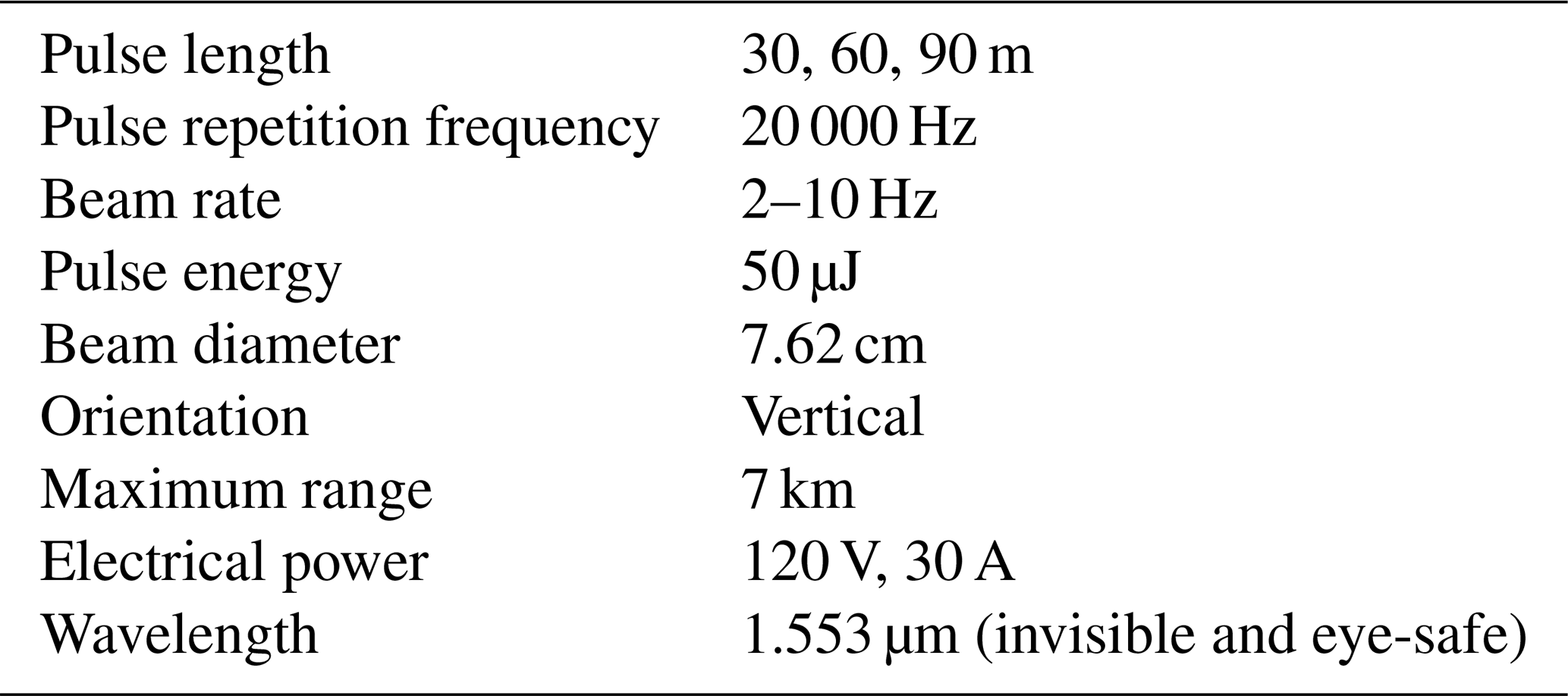
The MD3 design was optimized for operation from pickup trucks and ships. The small modular footprint and weight of all subsystems allow their positioning in various compact spaces and enable easy stabilization. The MD3 lidar system features two laser transmitters and two channels to provide both continuous vertical-stare profiles of the vertical velocity w and, simultaneously, azimuth scans at 15° off-zenith to give profiles of the horizontal wind speed and direction using the velocity-azimuth display (VAD) technique (Browning and Wexler, 1968; Banta et al., 2002). The ability to do azimuthal scans at lower elevation angles, which can enhance accuracy in the horizontal VAD wind estimate (see Banta et al., 2023), is currently under development. The technical specifications of the MD3 lidar are given in Table 1.

Table 1 Typical specifications of the MD3 lidar.

Many portable configurations of remote sensing instruments currently used for various applications, including weather and atmospheric research, such as the Collaborative Lower Atmospheric Mobile Profiling System (https://www.nssl.noaa.gov/tools/clamps, last access: 12 November 2024), are considered “mobile” systems. However, these systems must be delivered to the location of interest to provide a stationary measurement or be used in a “go-and-stop-for-measurements” pattern. In contrast, the mobile MD lidars developed at CSL/NOAA (Fig. 1a–c) provide continuous measurements of w and horizontal winds while the platform is moving, which is a significant advantage compared to the constraint of stationary Doppler lidars to obtain vertical and horizontal wind profiles at one location.

The truck-based measurements provide profiles of wind speed, wind direction, w, and aerosol backscatter intensity, showing the wind flow variability in time, with height, and along the moving path.

Figure 1 NOAA/CSL mobile Doppler lidar systems: (a) ship-based; (b) aircraft-based; (c) truck-based.

The mobile lidar measurements have been used for various environmental studies. The multi-platform (aircraft and ground-based) setup was successfully used during recent wildfire and air-quality experiments, providing a unique opportunity to characterize atmospheric processes, including studies of fire plume transport dynamics, in better detail (Carroll et al., 2024; Strobach et al., 2023, 2024). The combination of spatial and temporal coverage of the aircraft-based mobile lidar measurements provides an advantage over traditional in situ or stationary profiling observations offshore and inland, for example, to study the air quality of large urban areas (https://csl.noaa.gov/projects/aeromma/cupids/, last access: 6 March 2024). In the summer of 2024, the aircraft and truck-based modifications were involved in multi-institutional projects to estimate emissions of methane, greenhouse gases, and other significant air pollutants from oil and gas production facilities located in urban and agricultural areas of Colorado (https://csl.noaa.gov/projects/airmaps/, last access: 22 May 2025). Table A1 in Appendix A shows a list of the CSL/NOAA field projects using mobile MD lidar on various platforms. The results obtained from these experiments use the high precision and excellent pointing accuracy of measurements from the ground-based, airborne, and shipborne deployments and demonstrate success in developing a fully capable mobile Doppler lidar for environmental studies.

Truck-based mobile lidar system

The latest version of the truck-based lidar system (Fig. 2), the PickUp-based Mobile Atmospheric Sounder (PUMAS), was recently used to study the spatial structure of horizontal wind and turbulence near wind farms in Colorado and northern central Oklahoma.

Figure 2 (a) Picture of PUMAS with indicated subsystems: motion-stabilization frame, lidar head, all-sky camera, and the sensor for in situ measurements of temperature (T^o) and wind speed; (b) the electronics rack located in the back of a cabin; (c) real-time display located in the front of the cabin.

The PUMAS system (Fig. 2a) included a motion-stabilization frame, the MD3 lidar head, an all-sky camera, and sensors for in situ temperature (T) and wind speed measurements. The electronics rack is located in the back of the cabin (Fig. 2b), and the real-time display is in the front of the cabin (Fig. 2c). PUMAS provided continuous motion-compensated measurements of wind flow and turbulence profiles driving on highways and dirt roads within wind farms. The two motion-stabilized lidar beams – vertically pointed and conically scanning with ±15° of zenith – provided simultaneous profiles of horizontal wind vectors, aerosol backscatter intensity, and w statistics from 60 m a.g.l. to the top of the atmospheric boundary layer under normal atmospheric conditions and absence of precipitation. Data were obtained with a temporal resolution of 1–4 Hz and an along-beam resolution of 30 m. Wind speed profiles were obtained with an along-path resolution of 300–600 m, and w profiles were obtained every 10–30 m. Along-path resolution depends on the driving speed and the road conditions but can be modified by changing accumulation time or scan settings in the real-time display software.

During several pilot studies, PUMAS was tested around wind farms in Colorado (Appendix B, Fig. B1) to obtain information on system performance, measurement errors, and driving strategies. The analysis of data from these test drives helped to set the science goals and a measurement strategy for the participation of PUMAS in the AWAKEN campaign.

3 American Wake Experiment

The AWAKEN campaign is a US Department of Energy (DOE) project led by the National Renewable Energy Laboratory (NREL). It is a multi-institutional, long-term (2021–2025) study in the US Great Plains aiming to understand the interaction between wind farms and their surrounding environment and to improve the performance of wake models. Wind farms in the northern central Oklahoma study area are located over relatively flat terrain (Fig. 3a). More information on the AWAKEN goals can be found here: https://openei.org/wiki/AWAKEN (last access: 18 January 2024). Participating organizations deployed various in situ and remote sensing instruments to the study area, including 14 stationary scanning Doppler lidars and 7 wind-profiling lidars. The full description, measurement objectives, and locations of the AWAKEN instrumentation can be found in the overview paper (Moriarty et al., 2024). The first benchmark study within the International Energy Agency Wind Task 57 framework focused on wind plant wakes (Bodini et al., 2024). Detailed information on the coordinated measurements from in situ and remote sensing instruments, including turbine nacelle-mounted lidars, is provided in AWAKEN-related papers (Bodini et al., 2024; Debnath et al., 2022, 2023; Krishnamurthy et al., 2021, 2025; Letizia et al., 2023; Moriarty et al., 2024). The long-term measurements from scanning lidars (Newsom and Krishnamurthy, 2020) at the Atmospheric Radiation Measurement (ARM) Southern Great Plains (SGP) and AWAKEN sites provide additional information on wind and turbulence in the surrounding area (Moriarty et al., 2024).

To support the AWAKEN science objectives, the CSL/ARS team operated PUMAS to provide motion-compensated measurements of 3D wind flow and turbulence profiles from 15 August to 12 September 2023. The measurements were mainly taken within and around the King Plains wind farm (Fig. 3), which comprised 88 General Electric wind turbines with a rated capacity of 2.82 MW, a hub height of 89 m, and a rotor diameter of 127 m.

Figure 3 Wind farms in northern central Oklahoma are shown on the terrain elevation map (Debnath et al., 2022) by black dots. Turbine symbols show King Plains wind farm to underline the research focus on this area. Red circles indicate the ARM SGP highly instrumented Central Facility C1 and the extended facility E37 (https://www.arm.gov/capabilities/observatories/sgp, last access: 12 November 2024). Pink and cyan pins indicate AWAKEN lidar and ASSIST sites used in this paper. The roads (transects), covered by PUMAS during AWAKEN, are shown by dark-red circles where each circle represents a profile measurement from 64 m up to several kilometers a.g.l. The white triangle indicates the Woodring Regional Airport in Oklahoma, located about 8 km southeast of the central business district of Enid, Oklahoma. This figure is created using map data © Google Earth 2023.

By considering the predominant wind direction estimated from various model forecasts at the Enid Woodring Regional Airport in Oklahoma, a driving plan for each day was designed to sample waked and free flows at various distances from the wind turbines (Fig. 3). Transects were repeated several times during 5–6 h of measurements each day. At the beginning and end of each transect, 5 min measurements were taken in a stationary position, and these data were used to evaluate the system performance, as shown in Sect. 3.3.

In addition to PUMAS measurements, data from stationary Doppler lidars deployed at various AWAKEN sites (Fig. 3) were used for this paper. Data from the PNLL flux station were used to estimate near-surface stability. Temperature and water vapor mixing ratios were estimated through the TROPoe retrieval (Turner and Blumberg, 2018; Turner and Loehnert, 2014) based on observations from the NREL ASSIST-II spectroradiometer (Michaud-Belleau et al., 2025) measurements at Site B (Fig. 3). A list of instruments used in the paper is given in Table 2.

Table 2 Coordinates of sites and types of instruments used in the paper.

3.1 Meteorological conditions during PUMAS measurements in northern Oklahoma

According to the Oklahoma Climatological Survey (https://www.ou.edu/ocs/oklahoma-climate, last access: 5 December 2024), the AWAKEN study area is in the North Central climate division. This northern section of the state is less influenced by the warm, moist air moving northward from the Gulf and experiences less cloudiness and precipitation compared to the southern and eastern portions of the state. Still, summers there are long and usually quite hot.

The surface wind statistics at the Enid Woodring Regional Airport, located 6.4 km southeast of downtown Enid, show predominant south-southeast wind directions in August and September 2023 and 5 m s⁻¹ mean winds with occasional gusts up to 10 m s⁻¹. The frequency of weak (1–4 m s⁻¹) winds is high for both months (71 % in August and 63 % in September), whereas stronger winds (4–11 m s⁻¹) were less common (17 % in August and 25 % in September). The August–September 2023 average temperature in Enid was 86–93 °F (30–34 °C) for the daytime and 68–73 °F (20–23 °C) for nighttime, with 20–22 sunny days each month and 2 rainy days on 13–14 September (http://www.windfinder.com/windstatistics/enid_woodring_regional_airport, last access: 5 December 2024).

The ARM SGP atmospheric observatory with various in situ and remote sensing instrument clusters is located in northern central Oklahoma and southern Kansas near the AWAKEN study area (Fig. 3). The scanning Doppler HALO Photonics lidars provide long-term wind and turbulence measurements (Newsom and Krishnamurthy, 2020) at the SGP central facility, C1, and four extended sites (E32, E37, E39, E41) and are used in many studies and experiments such as the Plains Elevated Convection at Night field campaign (Geerts et al., 2017) or the Land–Atmosphere Feedback Experiment (Wulfmeyer et al., 2018; Pichugina et al., 2023, 2024).

A 6-year analysis of (2013–2019) Doppler lidar data at C1 located north of the King Plains wind farm (Fig. 3) confirms predominant southeast and south-southeast wind directions at 91 m a.g.l. in August and September (Krishnamurthy et al., 2021). Another detailed study of winds from Doppler lidars at the five SGP sites revealed that the interannual (2016–2022) variability in monthly mean summer nighttime winds in the layer of 700 m a.g.l. was more significant (4 m s⁻¹) compared to the wind variability (1–3 m s⁻¹) between sites, which are separated by 56–77 km, characterized by different vegetation types, and have elevations that vary between 279 and 379 m above sea level (a.s.l.) (Pichugina et al., 2023). They also reported predominant south-southeast nighttime winds at all sites and frequent wind maxima at ∼300 m.

Figure 4 Wind roses of 91 m winds from Doppler lidars at the ARM SGP sites (a) C1 and (b) E37 for all hours of measurements during 15 August–12 September 2023. (c, d) Time–height cross-sections of period-mean wind speed (colors) and wind direction (arrows) from each Doppler lidar. Local time = UTC−5.

Wind roses of 91 m winds from stationary Doppler lidar measurements from 15 August–12 September 2023 at two ARM SGP sites (C1 and E37) closest to the King Plains wind farm show wind directions from north to southwest with predominant southeasterly winds (Fig. 4a, b). Time–height cross-sections of winds averaged over 15 August–12 September 2023 (Fig. 4c, d) were moderate (8–12 m s⁻¹) at night and weaker (4–6 m s⁻¹) during the daytime. At both sites, wind directions below 300 m were primarily southeasterly, with some episodes of southerly winds at higher elevations. At C1 (Fig. 5c), LLJ development is evident within 200–700 m a.g.l. around ∼05:00–12:00 UTC, whereas at the western E37 site, located 51 km to the southwest of C1 (Fig. 3), the LLJ developed earlier in the 100–700 m layer.

Figure 5 (a) Diurnal distribution of the PUMAS hours of operation during AWAKEN; (b) wind rose of turbine-level (64–160 m) winds from the PUMAS measurements.

3.2 Statistics of PUMAS measurements

As mentioned, PUMAS participated in the AWAKEN experiment from 15 August to 12 September 2023. Only 20 d of good measurements were available due to poor weather conditions (heavy rain) and technical issues such as flat tires or lidar system component issues. In total, 4 d were spent on a round trip between Boulder, Colorado, and Enid, Oklahoma. During each 982 km one-way commute, PUMAS provided continuous measurements of wind speed, wind direction, and w. The system performance was monitored and corrected as needed in real time, including motion-compensation parameters such as transceiver pitch, roll, and heading; platform velocity and coordinates; and estimates of the lidar beam azimuth and elevation in a world reference frame.

Overall, during the 20 driving days, PUMAS was on the road 81 h, covering 3930 km (2443 mi) and providing 16 955 profiles of horizontal winds and w excluding data obtained during Denver–Oklahoma commutes.

The distribution of PUMAS operation hours (Fig. 5a) shows that the most intense measurement period was in the late morning to midday (15:00–20:00 UTC). Nighttime measurements during stable conditions, when turbine wakes could be better observed due to the more substantial wind speeds and lower turbulence, were limited by the country road conditions and poor visibility of the upcoming crossroads traffic. It was expected that some events, such as the nocturnal LLJ, a frequent Great Plains phenomenon (Banta et al., 2002), would not be captured in the late mornings. However, the dissipation times of the LLJ often depend on synoptic conditions, and in some cases, LLJ can be observed after sunrise hours (Carroll et al., 2019; Squitieri and Gallus, 2016; Pichugina et al., 2023).

The wind rose of the 64–160 m layer wind speeds (Fig. 5b) shows the dominance of southeasterly winds during PUMAS measurements. Strong (>15 m s⁻¹) winds were observed in 13 % of the southerly cases, followed by 10 % in southeasterly and 7 % in southwesterly directions. Based on the $d\mathit{\theta }/\mathrm{d}z$ data from the ASSIST at Site B, the majority of PUMAS measurements were taken under unstable conditions (88.3 %) as estimated from the ASSIST measurements at Site B. Stable conditions were observed in 7.8 % of cases, and near-neutral conditions were observed in 3.9 % of cases.

3.3 Platform stabilization and motion correction

Active stabilization and pointing correction, implemented in the mobile lidar system, compensate for truck motions such as pitch and roll (Fig. 6a, b) removing the effect of bumps on w while PUMAS is moving. In other words, the stabilization and motion-corrected system allow measurements of the w to be obtained without contamination from the projection of the horizontal wind speeds and their variation. Correction of the pitch and roll motions keeps the lidar beam elevation angle in a world frame at 89.21° on average with a standard deviation of ±0.96 (Fig. 6c) to obtain corrected line-of-sight velocity with an accuracy of $-\mathrm{0.04}\pm \mathrm{0.31}$ m s⁻¹. An example of the motion-corrected vertical velocity from PUMAS measurements on 7 September (Fig. 6e) shows significant turbulence in the first 1 km a.s.l. and illustrates the 287–415 m variability in the terrain covered by PUMAS on this day. The mean difference between measured and motion-corrected w at 105 m (Fig. 6f) is 0.08±0.32 m s⁻¹.

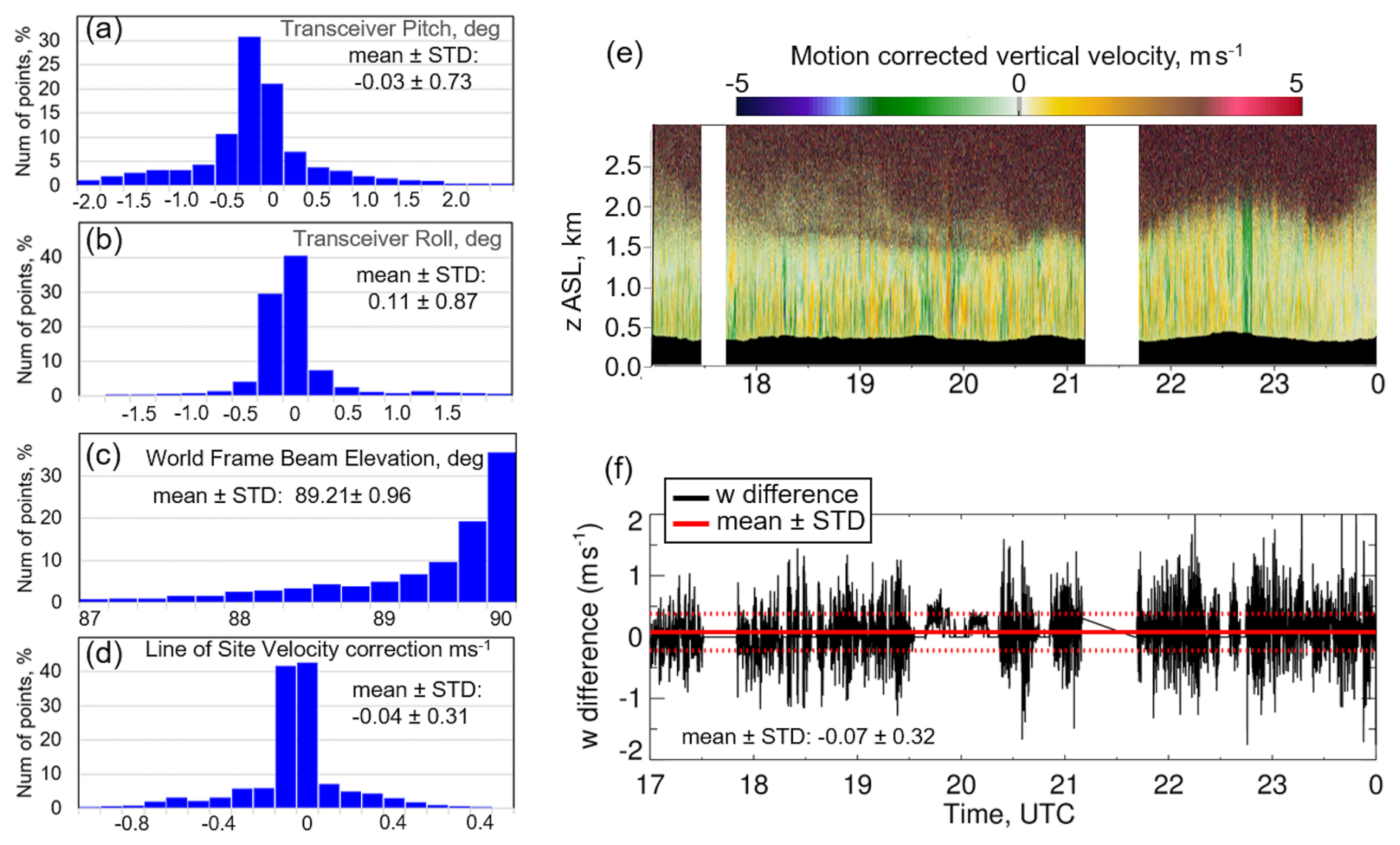
Figure 6 (a–d) Distributions (%) of the truck motion correction from PUMAS vertical velocity measurements from 15 August–12 September 2023, during AWAKEN. Mean ± standard deviation (STD) is shown on the panel for each parameter. (e) A sample of motion-corrected vertical velocity measurements from 17:00 to 24:07 UTC on 7 September 2023. Terrain elevation above sea level (a.s.l.) covered by PUMAS on this day is shown in black. The white areas indicate missing data. (f) Time series of a (black) difference between measured and motion-corrected vertical velocity on 7 September 2023 at 105 m above ground level (a.g.l.). The solid red line shows a period-mean difference. Dotted red lines show STD from the mean.

As mentioned, PUMAS provided 5–7 min of measurements in a stationary position at the beginning and end of each transect. Measurements collected by PUMAS in a stationary position or while driving within a 2 km radius of a DOE stationary lidar at Site A1 or H are used to estimate the accuracy of PUMAS's horizontal wind speed and direction by comparing the PUMAS and DOE lidar measurements as shown in Fig. 7 and summarized in Table 3. The different number of wind speed and direction points (count) for each case is because the 3σ outlier rejection (see Pichugina et al., 2019, 2020) to the 1:1 fit was applied for speed and direction separately, leading to a different number of outlier points removed for speed and for direction. High correlation coefficients were obtained for wind speed (0.83–0.96) and wind direction (0.93–0.99) from PUMAS measurements in a stationary position and while moving, except two cases when correlation coefficients were 0.65 between wind speed from the stationary PUMAS and Doppler lidar at Site A1 and 0.62 between wind direction from the moving PUMAS and Doppler lidar at Site H. A larger offset in wind direction histograms was observed between PUMAS and Doppler lidar at Site H. Detailed analysis of these results is beyond the scope of this paper.

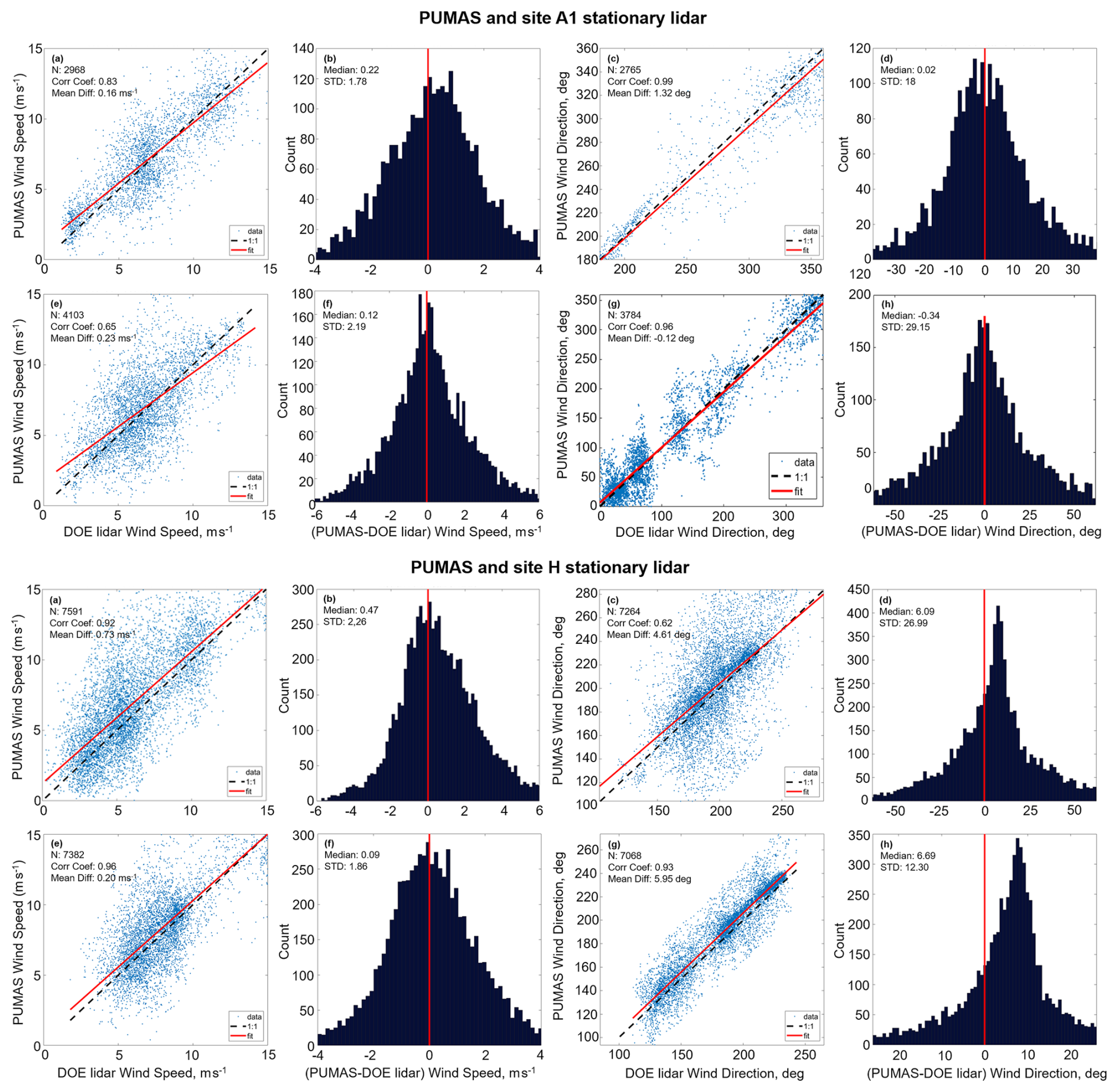
Figure 7 Comparison of horizontal wind and direction between PUMAS and DOE stationary Doppler lidar at sites A1 and H: (a–d) from PUMAS measurements in stationary position collected within 2 km radius from DOE stationary Doppler lidar; (e–h) from moving PUMAS measurements collected within 2 km radius from DOE stationary Doppler lidar.

Table 3 Statistics from the comparison of wind speed and direction measurements from PUMAS and stationary Doppler lidars.

Overall, Figs. 6 and 7 and Table 3 clearly illustrate success in developing a fully capable mobile Doppler lidar that compensated for the truck's motions to provide accurate wind measurements. The uncertainty of the horizontal wind speed and direction estimated by the VAD technique (Banta et al., 2013a) from PUMAS line-of-sight velocity measurements during AWAKEN was found to be very small with mean and standard deviations of 0.014±0.008 m s⁻¹ for wind speed and 0.12±0.18° for wind direction. The accuracy of motion-compensated measurements from mobile lidars was tested against stationary Doppler lidar measurements during several field campaigns. Examples of active stabilization and the accuracy of diurnal measurements from ship-based lidar during the offshore VOCALS campaign (Table A1) are provided in the Supplement (S1a, b). Examples (S2a, b) illustrate a high correlation for wind speed (0.89, 0.90) and direction (0.93, 0.99) obtained from two experiments while PUMAS was driving within a 2.5 km radius from the stationary lidar (S2c) and when PUMAS provided measurements in a stationary position for several months (S2d).

4 5 and 7 September case studies: fixed-site context measurements

Two days, 5 and 7 September, were selected to illustrate the PUMAS measurements and analysis techniques. The data on these days were obtained during morning transition (5 September) and day–evening transition (7 September) periods, characterized by some difference in wind conditions and BL stability. In this section we characterize the boundary layer evolution on these days based on fixed-location sensor measurements. Figure 8 shows wind speed (Fig. 8a, c) and direction (Fig. 8b, d) on these days from stationary Doppler lidars at SGP Site C1 (left) and SGP Site E37 (right).

Figure 8 Time–height cross-sections of wind speed and wind direction from stationary lidar measurements at the SGP sites C1 (left) and E37 (right) on (a–d) 5 September and (e–h) 7 September 2023. Black lines indicate periods of PUMAS measurements on these days. The temporal resolution of lidar data at C1 is 15 min, and that at E37 is 10 min. Lidar data at SGP sites can be found in the DOE ARM archive (Shippert et al., 2010, 2016).

4.1 Wind speed and direction from stationary Doppler lidars

On 5 September (Fig. 8a, b), during a period of PUMAS operations in the early morning hours (11:43–16:45 UTC, 05:43–10:45 LST), both SGP lidars show strong (15–25 m s⁻¹) wind speeds and the development of the LLJ at 02:00–15:00 UTC (LST = UTC−5 h) with the LLJ maximum at 600 m. Wind directions (Fig. 8c, d) in the first 200–300 m a.g.l. changed from southeasterly at nighttime, veering to southwesterly from late morning to afternoon and becoming northerly in the evening hours (after 18:00 UTC). The wind speed ramp-down event observed at ∼09:00–11:00 UTC below 400 m is most likely another example of an atmospheric bore, as analyzed in this region by Pichugina et al. (2024). It corresponds to a transient shift to a more southwesterly wind direction. Such significant increases or decreases in wind speed lasting for 30 min or more are difficult to forecast but may significantly affect turbine operations.

On 7 September (Fig. 8e–h), both SGP lidars showed weak (<4 m s⁻¹) nighttime winds that increased to 8–12 m s⁻¹ by 09:00–10:00 UTC (Fig. 8c). The LLJ of ≥15 m s⁻¹ developed at Site C1 at 14:00–15:00 UTC below 400 m, while stronger (15–20 m s⁻¹) LLJ developed at Site E37 around 13:00–15:00 UTC below 300 m. Wind directions (Fig. 8g, h) were primarily east-southeasterly (100–150°) at both sites.

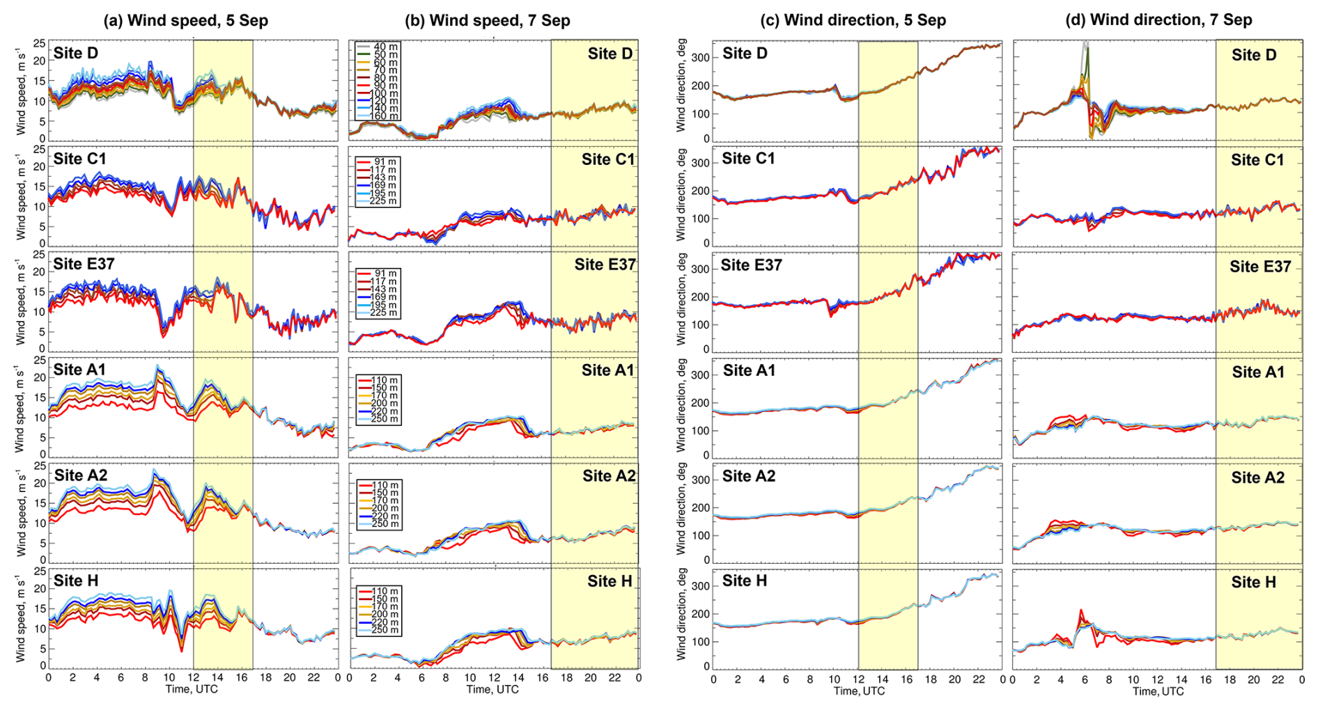
Figure 9 Time series of (a, b) wind speed and (c, d) wind direction from six stationary Doppler lidars at lowest heights on 5 and 7 September. Locations of lidar sites (Site D, Site C1, Site E37, Site A1, Site A2, and Site H) are shown in Fig. 4. The heights of measurements are indicated in the legend for each lidar. Periods of PUMAS operations on 5 and 7 September are highlighted in yellow.

Time series of wind speed and direction (Fig. 9) at the six lowest heights from all stationary lidars depicted in Fig. 4 also show similar trends in the evolution of wind flows, despite a significant distance between these instruments and locations at different terrain over the AWAKEN research area (Fig. 4). In Fig. 9, all lidars show highly variable wind speeds on 5 September, with indications of the ramp event (bore) around 09:00–12:00 UTC and weaker, less variable winds on 7 September.

Interestingly, this pattern changed little between lidar measurements of inflow at Site A2 and waked flow at Site H during the period of PUMAS measurements highlighted in yellow (Fig. 9). On 5 September, the mean wind speed at Site A2 was 0.8 m s⁻¹ larger, and on 7 September, mean winds were 0.46 m s⁻¹ weaker compared to Site H. The difference in wind direction between sites was 6.39° on 5 September and 7.83° on 7 September.

4.2 Stability on 5 and 7 September 2023

The virtual potential temperature (θ_v) computed from the TROPoe retrievals (Turner and Loehnert, 2014) of temperature and water vapor mixing ratio from thermodynamic profiler (ASSIST) data at Site B is shown (Fig. 10a, b) for 5 and 7 September. The time–height cross-sections show cooler temperatures near the surface prior to 16:00 UTC and warmer daytime surface temperatures after 17:00 UTC, as well as the growth of the convective layer (black line) after 15:00 UTC, on both days. Stability estimates based on the virtual potential temperature gradient ($\mathrm{d}{\mathit{\theta }}_{\mathrm{v}}/\mathrm{d}z$) show stable conditions at the beginning of PUMAS measurements on 5 September that changed to unstable by the end of the period (Fig. 10c), whereas on 7 September, the unstable conditions were observed during all hours of PUMAS operations (Fig. 10d).

Figure 10 (a) Virtual potential temperature (θ_v) from ASSIST data at Site B on (a) 5 September and (b) 7 September. Black lines show planetary boundary layer height (m) derived from the retrieved fields. Virtual potential temperature gradient ($\mathrm{d}{\mathit{\theta }}_{\mathrm{v}}/\mathrm{d}z$) on (c) 5 September and (d) 7 September at 10 m a.g.l. and three heights within the limits of turbine blades. Shaded gray areas indicate periods of PUMAS measurement on each day.

5 PUMAS measurements on 5 and 7 September 2023

The PUMAS data, obtained with high temporal resolution and a significant spatial distribution over driving transects (see the following subsections), show a similar evolution of wind speed and direction to the stationary SGP lidars (Fig. 8) for the period of PUMAS operations.

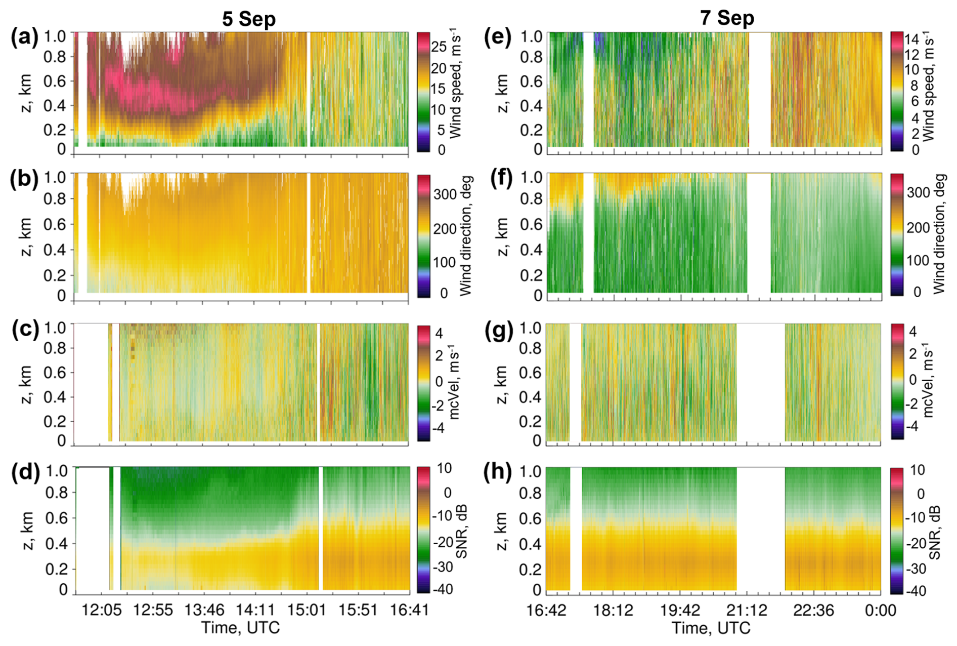
Figure 11 PUMAS-measured time–height cross-sections of (a, e) wind speed, (b, f) direction, (c, g) motion-corrected vertical velocity, and (d, h) SNR (signal-to-noise ratio) intensity from simultaneous (a, b, e, f) scanning and (c, d, g, h) vertically pointing data on 5 September (left column) and 7 September (right column). White areas indicate missing data.

On 5 September (Fig. 11a–d), PUMAS measurements in the morning hours (11:43–16:45 UTC) show an LLJ mixing out after 15:00 UTC. The data captured strong (≥15 m s⁻¹) morning (∼12:00–15:00 UTC) wind speeds at higher elevations and the LLJ of ∼25 m s⁻¹ at 500–600 m (Fig. 11a). The wind directions were predominantly south-southwesterly (∼200°) with short periods of southerly winds below 200 m (Fig. 11b). Stronger convective mixing was observed after 15:00 UTC (Fig. 11c) as BL depth increased from 400 to 600 m a.g.l. (Fig. 11d) and stability within rotor heights changed from stable to unstable (Fig. 10c).

On 7 September (Fig. 11e–h), PUMAS operated in the field for about 7 h from late morning to the evening (16:42–00:07 UTC). Similarly to 5 September, the agreement in trend (wind speeds increasing through the period) between data from stationary SGP lidars and PUMAS measurements was evident, although PUMAS sampled somewhat weaker winds. The daytime (16:42–21:00 UTC) southeasterly (120–140°) winds of 5–8 m s⁻¹ increased by the evening to 10–12 m s⁻¹ (Fig. 11e) and veered to south-southeasterly (160–170°) below 600 m (Fig. 11f). The steady mixing with the BL height to >600 m was observed during most of the period (Fig. 11g, h) characterized by the unstable BL conditions (Fig. 10d).

The next sections will provide a closer look at PUMAS measurements during selected days starting with 7 September, the longest period of measurements characterized by moderate (6–12 m s⁻¹) wind speed and unstable BL conditions, which were common for most days during PUMAS operations.

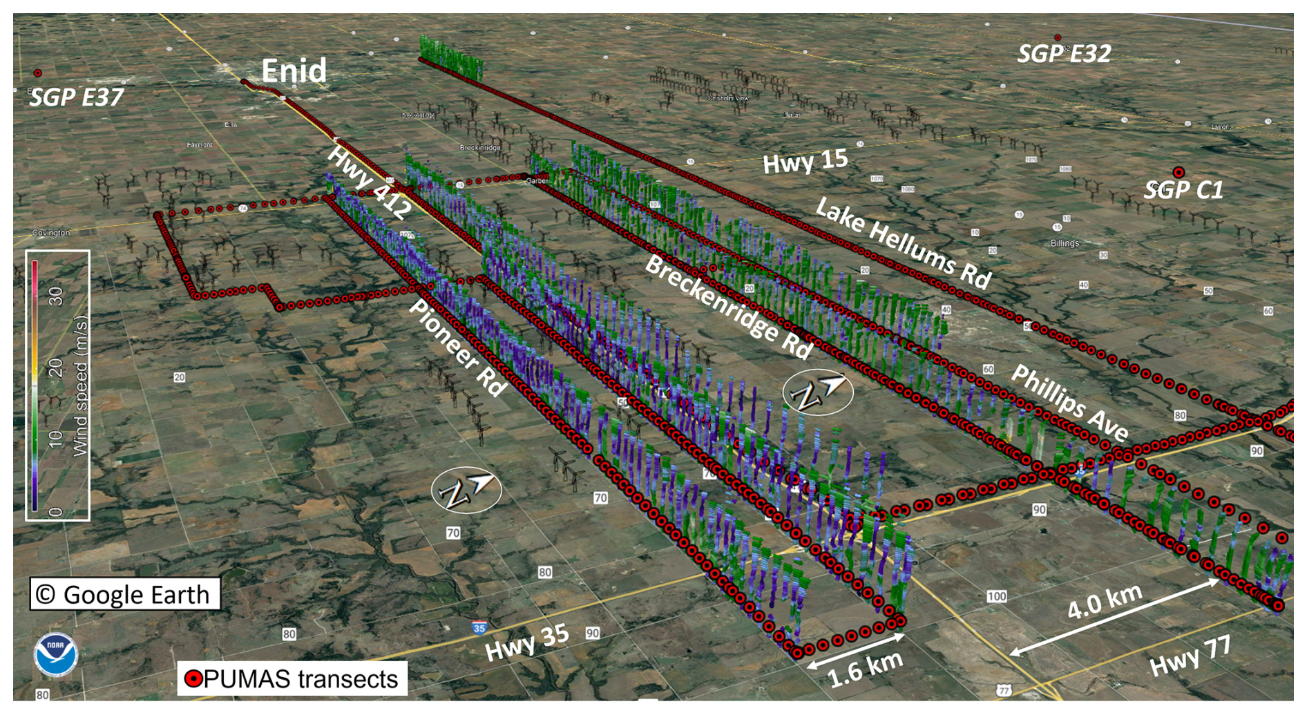
Figure 12 Samples of wind profiles along some transects on 5 September 2023, embedded on Google Earth, are rotated clockwise ∼45° for a better view. Profiles are shown up to 1.5 km a.g.l., and wind speed is scaled from 0 to 30 m s⁻¹ according to the color scale on the left side of this figure. The horizontal distance between profiles is about 300 m. White arrows indicate distances between illustrated transects along the named roads. Gray circles indicate the ARM SGP sites (C1, E37, and E32). Figure 12 is created using map data © Google Earth 2023.

5.1 7 September case study, southeasterly winds

Throughout the previous sections, 5 September was discussed first, then 7 September. Here, we change the order and start with the case study on 7 September, as it was the longest period of PUMAS measurements, and these data were taken during the most frequently sampled (Fig. 5a) late-morning (16:00–20:00 UTC) hours. Relatively calm wind speeds and southeasterly directions on this day are more typical of many other AWAKEN days (in contrast to the 5 September case of strong southwesterly winds). On 7 September, PUMAS operated in the field for 7 h and 25 min (16:42–00:07 UTC), covering more than 422 km. A 3D visualization of wind profiles (Fig. 12) measured on 7 September along several transects, out of 34 total for the day, illustrates stronger (≥10 m s⁻¹) winds in green compared to weaker (≤5 m s⁻¹) winds in purple.

5.2 Technique to estimate free and waked flows

A technique to estimate wind speed for sections of a transect that are in the shadow of wind turbines (waked flow) or free from the turbine influence (free flow) is based on the density of upstream wind turbines that may impact wind measurements, computed within 10 km from the road (Fig. 13b, e) including all Breckinridge wind farm turbines located within 2–4.7 km from this road (note a slight spelling difference in the road and wind farm names). This example did not consider some of the King Plains and all Armadillo Flats turbines located more than 10 km from the road. The influence of turbines on wind speed measurements (turbine shadow) was estimated within a 20° arc (±10° turbine shadow) upwind of each point of a PUMAS measurement of wind direction. Sections of a transect indicated by red in the wind time series (Fig. 13a, d) are considered waked, whereas those considered not influenced by wind turbines (free flow) are blue.

Figure 13a, d show time series of the rotor layer (64–150 m) mean wind speed measured during the east-to-west (EW; 59.2 km) and west-to-east (WE; 55.4 km) transects on Lake Hellums Rd. (Fig. 12). Mean rotor layer winds in the free flow sectors along the EW transect increased from 9.1 to 9.9 m s⁻¹, whereas on the return WE transect, the winds decreased from 8.9 to 8.2 m s⁻¹. The free flow wind speeds were thus stronger for the western sector by 0.7–0.8 m s⁻¹, most likely due to terrain differences, and the winds slowed by ∼1 m s⁻¹ in the time between the two sampling legs. Significant spatial variation in the wind speed within both the waked flow and the free flow sectors reflects the significant natural atmospheric variability characteristic of this midday convective period. These natural variations are thus larger than the mean-speed differences between waked and free flow regions, making the waked region hard to identify.

Figure 13 Time series of wind speed averaged over the rotor layer (64–159 m) height from PUMAS measurements on Lake Hellums Rd. during (a) east–west (49.3 min) and (b) west–east (54 min) transects. Blue indicates free wind flow that is not influenced by wind turbines, and red indicates waked wind flow. The density of Breckinridge and King Plains wind turbines is computed within 10 km from the PUMAS transects. (c, f) Mean wind speed and direction profiles at each transect for parts of (blue) free and (red) waked flows.

The mean profiles of free flow and waked winds are shown in Fig. 13c, f. Within the turbine layer, mean waked speeds were slightly (<1 m s⁻¹) larger than the mean free-wind values for the EW transect (Fig. 13c), contrary to expectation, but comprehensible in light of the variable nature of the convective boundary layer, as discussed in the previous paragraph. Within 200–400 m, these profiles are the same, deviating again at higher levels. During the WE transect (Fig. 13f), both free and waked profiles were very similar. Mean profiles of wind direction for waked and free winds are close for both EW and WE transects, turning from 140° within the rotor layer to 175° at 1 km a.g.l. The statistically insignificant difference between mean waked and free wind speed profiles in this example resulted from the temporal evolution of winds over 55 min drive one way.

Calculated from the data in Fig. 13a, the rotor-layer-mean waked flow from the Breckinridge wind farm was 8.8 m s⁻¹ compared to 10 m s⁻¹ of waked flow downwind of the King Plains wind farm (Fig. 13b). The difference in waked flow between the Breckinridge (8.7 m s⁻¹) and King Plains (8.3 m s⁻¹) wind farms is much smaller on the way back (Fig. 13d). As stated previously, these differences are primarily due to the temporal variability in wind speed and the slope of the terrain along Lake Hellums Rd., which descends from 400 m on the west to 280 m on the east.

Figure 14 Top row: mean profiles of (blue) free and (red) waked wind speed and direction from PUMAS measurements on (a) Hwy 412, (b) Breckenridge Rd., and (c) Phillips Ave. Yellow indicates inflow wind profiles from stationary Doppler lidar at Site A2 averaged for the corresponding time interval. Bottom row: mean wind speed and direction profiles (d–f) from stationary Doppler lidar measurements at sites (black) H, (blue) A1, and (yellow) A2.

The developed technique allows waked and free flows from measurements at different distances from turbines to be estimated as illustrated in Fig. 14 for the following transects: (Fig. 14a) within King Plains wind farm on Hwy 412; (Fig. 14b) on the Breckenridge Rd. located 0.9 km of the wind farm; and (Fig. 14c) on Lake Hellums Rd. located 5 km north of the turbines (Fig. 4). Profiles show free-stream winds at locations within the wind farm 1–1.5 m s⁻¹ stronger than waked winds there, as expected, and the difference decreases with distance from the farm, until, at 5 km (Fig. 14c), the waked and free flow profiles are equal within the standard deviation error, indicating that the wake has mixed out. Wind directions of waked and free flows at each transect (Fig. 14a–c) remain southeast below 500 m a.g.l. and turn to southwest at higher levels.

Fixed sites A2, A1, and H form a south–north line through the King's Plains wind farm. The lower panels of Fig. 14 show wind profiles at these three sites averaged for three time periods from late morning to late afternoon. For the first two time periods, the mean wind speeds at downwind Site H were larger compared to other sites (Fig. 14d, e), again contrary to expectation. Radünz et al. (2025) also noticed this effect and attributed the differences to terrain influences that can lead to increased wind speeds downwind.

Figure 14a–c show comparisons of PUMAS-measured wind profiles with those for stationary lidar Site A2. The PUMAS wind speeds are mostly within 1 m s⁻¹ of the A2 profiles, and the directions are very close (the A2 profile in Fig. 14a needs to be adjusted downward for the comparison due to terrain elevation differences), indicating good agreement. The spread between the mobile and fixed profiles is similar to the spread among the fixed sites shown in Fig. 14d–f.

The technique allows us to estimate the overall impact of individual wind farms as illustrated in Fig. 15. During the ∼55 km transect on Lake Hellums Rd., PUMAS passed Breckinridge and King Plains wind farms twice, going east to west and back (Fig. 13b, d). The difference in turbine layer wind flow downstream of both wind farms was about 1.3 m s⁻¹ during the EW transect due to a slight increase in wind speeds at 22:07–22:17 UTC (Fig. 15c). During the WE transect, winds downstream of both wind farms were almost equal with the mean difference of 0.36 m s⁻¹ (Fig. 15d). Wind directions in the rotor layer were close for both transects, with differences of 2°.

Figure 15 Wind speed and direction profiles from PUMAS measurement within the 10 km radius of influence by turbines from (gold) King Plains and (dark red) Breckinridge wind farms during (a) east-to-west and (b) west-to-east transects along Lake Hellums Rd. (Fig. 13). (c, d) Time–height cross-sections of wind speed at these transects. Color bars at the bottom of both panels indicate parts of each transect downstream of (gold) King Plains and (dark red) Breckinridge wind farms.

The results in Figs. 13–15 illustrate the ability to determine free and waked flows on long (>55 km) transects at various distances (0.9–5 km) from the wind farm and to compare the waked flow downwind of the Breckinridge and King Plains wind farms. These results are obtained for moderate (6–12 m s⁻¹) southeasterly winds and unstable BL conditions of large atmospheric variability and strong vertical mixing, leading to rapid mixing out of the wakes. Spatial variations in the free-stream wind speed, often related to small differences in terrain, and temporal changes were ∼1 m s⁻¹, which were similar to the differences between waked and free-stream speeds, when observed. Thus, under these daytime conditions, it was often difficult to distinguish the wakes from the ambient flow. The following section will show some examples from PUMAS measurements on 5 September characterized by stronger (10–20 m s⁻¹) wind speeds.

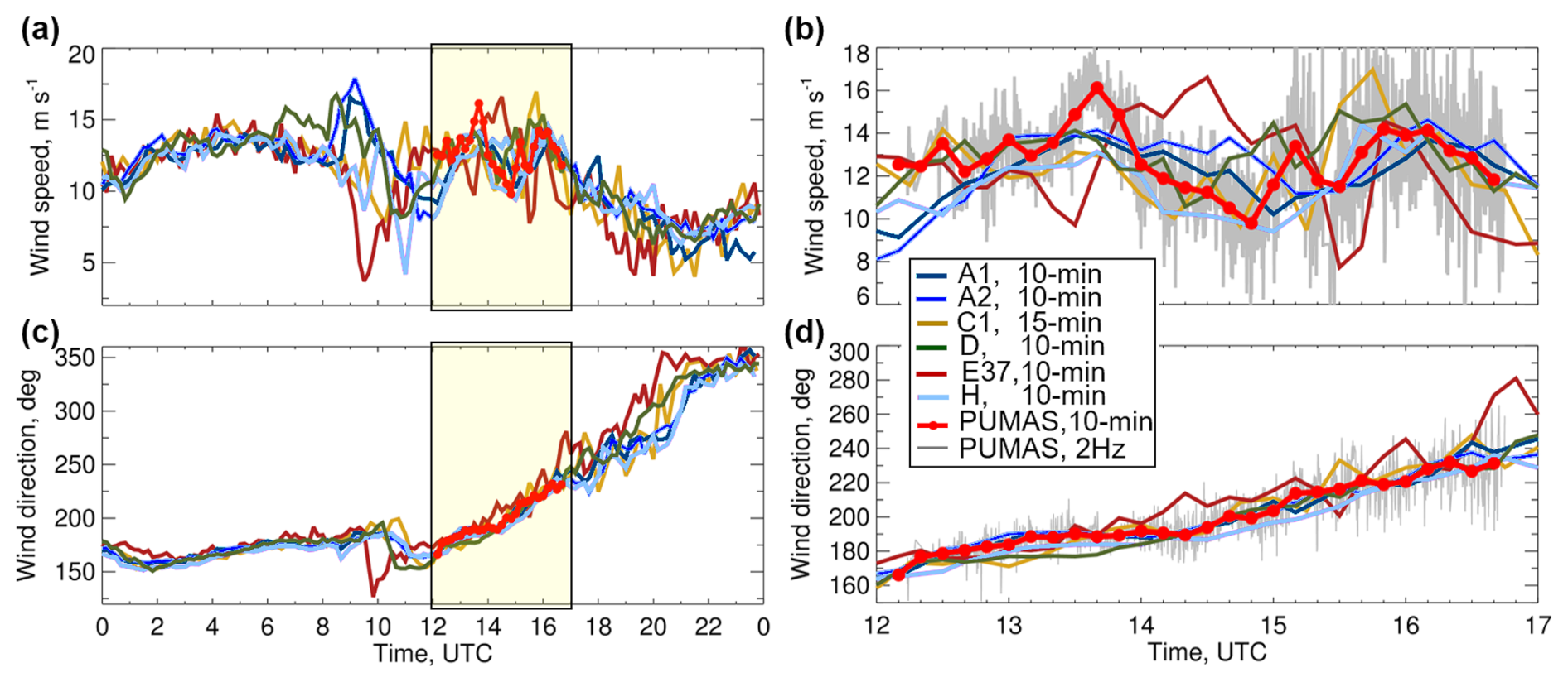
Figure 16 Wind speed and wind direction at 90–110 m from several AWAKEN stationary Doppler lidars and PUMAS on 5 September 2023: (a) time series of 10 min (15 min at C1) data from stationary lidars at several sites are shown for 24 h by colors according to the color scale. Data are taken close to the hub height: 90 m at sites C1, E37, D, and PUMAS; 110 m at sites A1, A2, and H. Yellow boxes indicate the time of PUMAS measurements on this day. (b) Same as panel (a) but for the period of PUMAS measurements at 12:00–17:00 UTC. Gray indicates 2 Hz PUMAS, and the red line with dots shows 10 min averages.

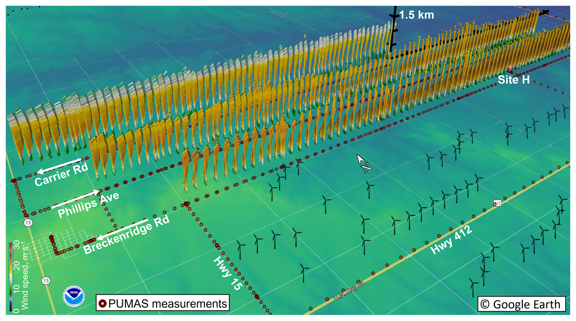
Figure 17 Wind speed (colors) and direction (arrows) profiles on 5 September are shown along individual transects on Breckenridge Rd. (13:14–13:34 UTC), Phillips Ave. (13:52–14:14 UTC), and Carrier Rd. (14:37–14:51 UTC) selected for the analysis. The dark-red circles indicate points of PUMAS measurements on 5 September. Profiles are embedded on a Google Earth terrain elevation map (Debnath et al., 2022) and rotated clockwise ∼60° for a better view. Wind speed is scaled from 0 to 30 m s⁻¹ according to the color scale on the left side of this figure. The horizontal distance between profiles is about 300 m. White arrows in the left corner indicate the PUMAS driving direction for each transect in this example. Figure 17 is created using map data © Google Earth 2023.

5.3 5 September case study, nocturnal LLJ, southwesterly winds

Time series of wind speed on 5 September from PUMAS and six stationary Doppler lidars (Fig. 3), taken at the heights closest to the turbine hub height of 90 m, are shown in Fig. 16 for the diurnal period (Fig. 16a) and the period of PUMAS operations (Fig. 16b). Wind speed and direction from all lidars show small differences and similar trends from sunset to midnight (01:00–06:00 UTC). Later in the morning and during PUMAS operations, winds at all sites fluctuate around 10–14 m s⁻¹, later decreasing to 5–8 m s⁻¹ by the evening hours. Wind directions from all lidars show steady turning from southeasterly (∼150°) to northerly (∼360°). Wind speed and direction for the period of PUMAS measurements at 12:00–17:00 UTC (yellow box in Fig. 16a, b) show similar variations in data from all lidars including PUMAS and close period-mean data (Table 4). Slightly lower (11.6 m s⁻¹) mean wind speed is observed at Site H, located in the wake of turbines for south-southwesterly directions compared to Site D (12.9 m s⁻¹) and Site A2 (12.4 m s⁻¹) of inflow lidar measurements (Table 4). The period-mean wind speed of 2 Hz (Fig. 16b, gray) and 10 min averaged (Fig. 16b, red) PUMAS measurements are similar (Table 4), but the standard deviation of 2 Hz data is larger (2.3 m s⁻¹) compared to the 0.4 m s⁻¹ standard deviation of 10 min averaged data.

Table 4 Mean and standard deviation of wind speed and direction from PUMAS and stationary lidars over the period of PUMAS operations on 5 September at 12:00–17:00 UTC.

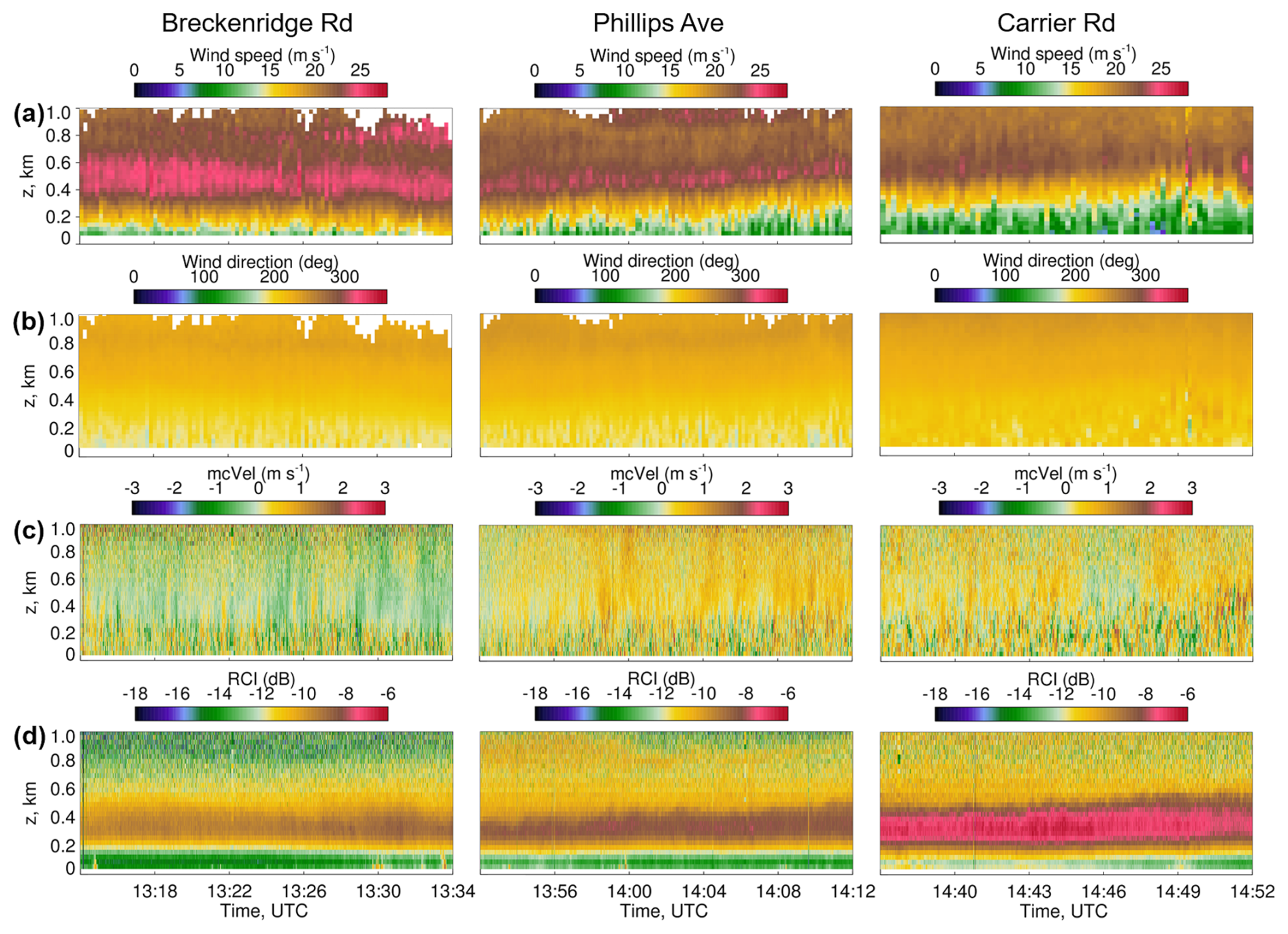
Figure 18 Time–height cross-sections of simultaneously measured (a) wind speed, (b) wind direction, (c) motion-corrected vertical velocity, and (d) range-corrected backscatter intensity from transects shown in Fig. 17 along (left column) Breckenridge Rd., (middle) Phillips Ave., and (right) Carrier Rd. Panels (c) and (d) are shown up to 1 km a.g.l. to illustrate BL growth.

An example of wind speed and direction profiles from PUMAS measurements within the King Plains wind farm is shown in Fig. 17 for 3 (out of 22 total) transects on 5 September. Transects are shown for alternate WE and EW driving directions on Breckenridge Rd., Phillips Ave., and Carrier Rd. (Fig. 17, white arrows). The south–north distance between these roads is 1.6 km. The length of these transects depends on road conditions and varies from 19.9 km on Breckenridge Rd. to 12.5 km on Carrier Rd., which ends due to the terrain after crossing County Road 20.

Time–height cross-sections (Fig. 18) of simultaneously measured wind speed, wind direction, and motion-corrected vertical velocity along the waked part of the transects from Fig. 17 illustrate temporal evolution of wind flows on each transect, as the convective BL mixed upward into the remaining nighttime LLJ. Wind speeds of 8–12 m s⁻¹ below 400 m increased to >25 m s⁻¹ above this height at all transects, with a strong (>28 m s⁻¹) LLJ within 400–600 m captured during the 20 min transect at Breckenridge Rd. The LLJ of ∼25 m s⁻¹, observed during the 20 min transect on Phillips Ave, decreased to 20 m s⁻¹ at the 15 min transect on Carrier Rd. Wind directions during all transects are mostly south-southwesterly (∼200°) with some episodes of southerly winds below 200 m (Fig. 18b). The motion-corrected vertical velocity is weaker at Breckenridge Rd. with more downward motions (Fig. 18c), but during all transects more variability is observed in the growing convective layer at low levels.

The temporal increase in BL depth can be seen in plots of vertical velocity (Fig. 18c) and the range-corrected intensity (Fig. 18d). Measurements from stationary lidars have been used extensively to estimate planetary boundary layer mixing height (Bonin et al., 2018), but a similar technique using mobile lidar measurements is currently under development.

The difference between waked and free flows in the rotor layer during all transects is less than 2 m s⁻¹ (Fig. 19a–c), and a similar difference for the same time intervals (Fig. 19d–f) is found between wind speed measured by stationary lidars at Site A2 (inflow) and Site H (waked). Although the mean wind direction within the rotor layer is south-southwesterly from PUMAS and stationary lidars during all transects, the BL stability changed from stable during the transect on Breckenridge Rd. to unstable during the transect on Carrier Rd. Wind speeds from PUMAS and three stationary lidars decreased with time but for all periods show high shear below LLJ maxima at 400–500 m. We note that the PUMAS profiles agree well with the fixed-site measurements when adjusted for terrain elevation differences, as we also found in Fig. 14.

Figure 19 Similar to Fig. 14 but for the mean profiles during transects on 5 September shown in Fig. 17.

6 Conclusions

Quantitative characteristics of wind and turbulence in the atmospheric layers occupied by the wind turbine rotor blades are crucial to wind energy, as is wind information above this layer to provide a meteorological context up to several hundreds of meters a.g.l. Understanding the variability in winds across wind farms and under different conditions is a key factor in the planning and operations of wind projects.

The high-frequency, motion-compensated PUMAS measurements of the horizontal wind speed, wind direction, range-corrected intensity, and simultaneous vertical velocity statistics (including variance, skewness, and kurtosis) from a moving platform provide a new approach to characterizing dynamic processes critical for wind farm wake analysis. The unique PUMAS measurements offer insight into the temporal and vertical variability in wind flows similar to stationary scanning lidars, and they also reveal spatial variability in the horizontal and vertical structure of wind flows modified by operating wind turbines.

In the daytime convective cases studied here, spatial variations in the unwaked, free-stream wind speeds were often ∼1 m s⁻¹, and temporal changes along transects repeated over periods of 1 h were of similar magnitude. Differences in waked vs. free-stream speeds, when discernable, were also ∼1 m s⁻¹, so it was often difficult to distinguish turbine or wind farm wake effects from the natural atmospheric variability under these conditions.

Data from the mobile lidar can also complement the AWAKEN instrumentation to understand the effect of a large wind farm on wind flows under different background wind conditions and stratification. The PUMAS measurements can be used to evaluate wind simulation models and improve wake model prediction accuracy. The truck-based mobile Doppler lidar data analyses show that advances in measuring, understanding, and modeling the atmospheric boundary layer within wind farms will be required to provide improved meteorological support for wind energy.

The developed technique allowed the sampling and automated analysis of wind speeds influenced by wind turbine clusters located at different distances from PUMAS transects and the flexibility to adjust the sampling drive patterns to account for any wind directions.

Limitations of the study and future research

The results presented in this paper are obtained from the short pilot study, mostly during daytime hours and low wind conditions. Therefore, we have not examined the higher orders of turbulence such as variance and skewness in this article, as we expect or already know that turbine wake effects would just be masked by daytime turbulence. In any case, the rich dataset obtained can be used for more analysis and future research papers, and it can contribute to the design of longer transects and driving patterns around wind farms. In addition, all data including time series of pitch, roll, lidar height (a.s.l.), and measured and motion-corrected vertical velocity are available for future detailed analysis. Ideally, future programs like AWAKEN will benefit from mobile platform measurements such as PUMAS to obtain long-term measurements of turbine wakes over various seasons and atmospheric events.

Appendix A: CSL/NOAA field projects in 2018–2024 using mobile lidar systems

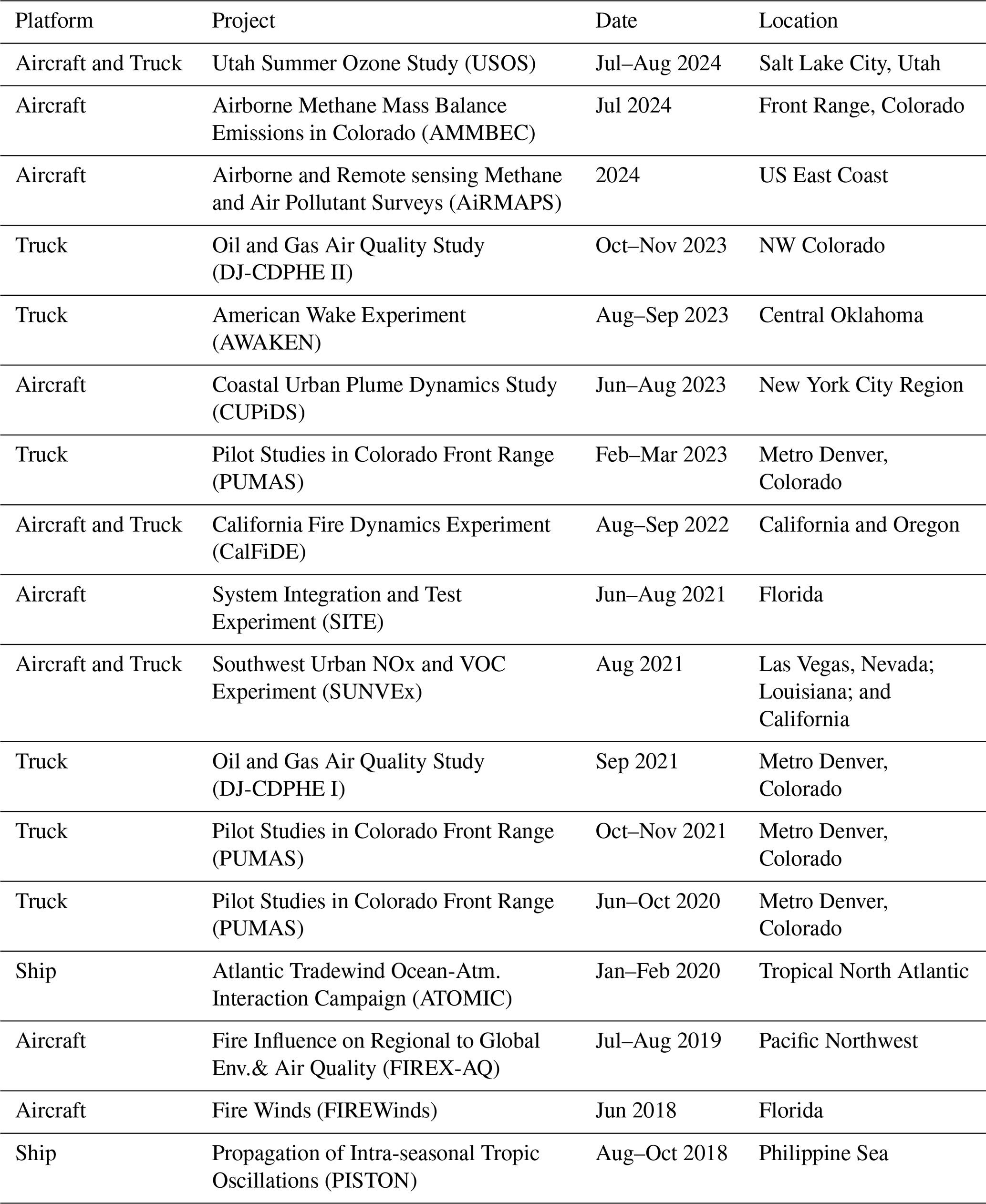
Table A1 Mobile Doppler lidar measurements from various platforms.

Appendix B: Test drives around wind farms in Colorado

Several test drives of PUMAS were performed around wind farms in Sterling and Limon located in the northern and southern parts of Colorado (Fig. B1a, b) to obtain information on system performance, measurement errors, and driving strategies. The data were used to establish measurement capability to study dynamic processes upwind and downwind of turbines. Figure B1c shows motion-stabilized vertical velocity obtained from a lidar beam pointing zenith (90° elevation angle).

The high temporal (∼20 s) and vertical (30 m) resolution of these profiles yields unique information about the extent and strengths of the vertical motions, including thermal updrafts and turbulence at the cloud base. Measurements from conical scanning at 15° from the zenith (Fig. B1d) reveal southerly wind speeds of ∼12 m s⁻¹ up to 1.5 km.

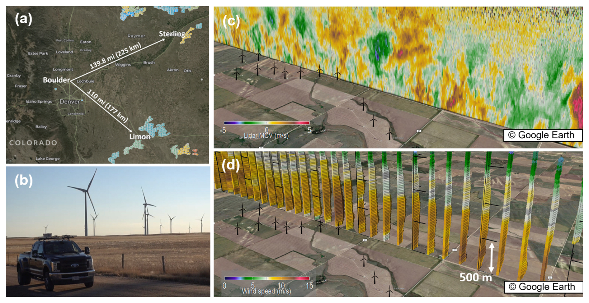
Figure B1 (a) A USGS map of wind farms located ∼200 km to the northeast (near Sterling) or to the southeast (near Limon) from Boulder, selected for PUMAS test drives in 2020, 2021, and 2023 (Table A1, Appendix A); (b) a picture of PUMAS driving in the vicinity of wind turbines; (c) profiles of vertical velocity along an ∼22 km path are shown on Google Earth; (d) profiles of wind speed (colors) and wind direction (arrows) along the same path. Black horizontal lines indicate height increments of 500 m. Panels (c) and (d) are created using map data © Google Earth 2023.