Validating wind farm parameterizations with offshore SCADA data

A large-scale validation compared wind farm parameterizations (WFPs) of the Weather Research and Forecasting (WRF) model to multi-year SCADA (supervisory control and data acquisition) data from six offshore wind farms. Although initially seven WFPs were considered, after preliminary assessment only three distinct ones were retained: the original Fitch (Fitch-O), a physics-derived axial-induction modification of Fitch (Fitch-pAIM), and the explicit wake parameterization (EWP). The study, conducted at 2 and 0.67 km resolutions, revealed total energy yield differences of ±5 % compared to SCADA data, with finer resolutions having a lower yield due to enhanced internal wake effects. The remainder focused on addressing the main sources of error affecting the total energy yield. The modeled mean wind speed was likely too low, leading to an energy yield underestimation. Only Fitch-pAIM accurately modeled the power curve and therefore the gross yield, while Fitch-O and EWP underestimated power by neglecting local induction effects. Internal wake magnitudes were well captured by Fitch-O and Fitch-pAIM at fine resolution, while EWP consistently produced wakes that were too weak. All WFPs showed signatures of global blockage and a dependency of wake losses on the vertical structure of the boundary layer. Lastly, external wakes were well captured by all parameterizations.

The results demonstrate that Fitch-pAIM outperforms other WFPs at resolutions smaller than the turbine spacing. Despite the limitations in accurately reproducing distinct wake features in aligned and staggered configurations, WFPs accurately capture the total wake loss, making their use suitable for annual energy production (AEP) calculations.

1 Introduction

One of the key aspects in the planning stage of a new wind farm is assessing the potential power production of a future site. For onshore sites this is typically done by erecting a met mast or deploying a lidar for several months to measure the local wind climate (Rohrig et al., 2019). For offshore sites, such measurement campaigns are considerably more expensive. To supplement the measurements, mesoscale models are often used, either by modeling individual sites of interest directly or by a previously generated atlas such as the New European Wind Atlas (Hahmann et al., 2020; Dörenkämper et al., 2020).

While the approach of correcting long-term model data sets with short measurement periods has worked well in the last decades, areas like the North Sea will see large changes in the near future with high densities of installed capacity, as offshore wind targets are set to 120 GW by 2030 and 300 GW by 2050 (EU, 2023). With this large number of installed capacity, wind farm or wind farm cluster wake effects will become even more relevant, and the influence of future neighboring wind farms on the expected power production of a new or existing farm needs to be accurately represented. As this future wake loss is not measurable before the farms are built, precise model solutions are essential.

The effect of the offshore wind farm wakes on the power production of downstream wind farms was first shown by Nygaard (2014) and Nygaard and Hansen (2016), demonstrating a drop in generated power of the Nysted wind farm after the upstream Rødsand II wind farm was commissioned. Since then, many studies have observed wind farm wake effects as a reduction in the wind speed or power using observations from met masts (Pettas et al., 2021), satellites (Christiansen and Hasager, 2005; Hasager et al., 2015; Ahsbahs et al., 2020), lidar (Schneemann et al., 2020; Cañadillas et al., 2022), radar (Nygaard and Newcombe, 2018; Ahsbahs et al., 2020), aircraft measurements (Platis et al., 2018; Cañadillas et al., 2020), and turbine data (Mittelmeier et al., 2017; Vollmer et al., 2024b; Sanchez Gomez et al., 2024). The magnitude of the impact of wind farm wakes on other wind farms is dependent on many factors like installed capacity density, distance between farms, and meteorological conditions. Lundquist et al. (2019) analyzed the economical impact of wake effects to be several million dollars for an onshore case study in the US and noted that there is no legal framework to protect existing wind farms. The high relevance of the topic is also evident from legal disputes between operators in the UK (Sanderson, 2025).

Engineering wake models like the Jensen (Jensen, 1983) or Gaussian model (Bastankhah and Porté-Agel, 2014, 2016) are historically the preferred tool for wind resource assessment. However, several studies have reported that such models tend to overestimate the recovery of the wind farm wake (Stieren and Stevens, 2021; Fischereit et al., 2022; Porchetta et al., 2026), although it should be noted that advances have recently been made (Nygaard et al., 2020; Souaiby and Porté-Agel, 2024). Microscale computational fluid dynamics models like large-eddy simulation (LES) models have been used for detailed studies on the physics involved (Stieren and Stevens, 2022) and due to computational advances are currently used at coarse resolution for annual energy production (AEP) estimates of wind farms (Baas et al., 2023). Due to their comparably low computational effort, the preferred modeling architecture to study wind farm wakes is by using mesoscale numerical weather prediction models, like the established Weather Research and Forecasting model (WRF; Skamarock et al., 2021). Siedersleben et al. (2018) compared WRF results with aircraft measurements and found good agreement of the spatial dimensions of the wake, while the magnitude of the simulated wake was sensitive to the background flow. By comparing to scanning lidar data, Cañadillas et al. (2022) demonstrated that the measured wind speed at a met mast inside a wind farm cluster was well represented when wind turbines are modeled in WRF. Studying cluster wakes, Montavon et al. (2024) found that turbine-to-turbine results are poor but that WRF performs well on the wind farm scale. In a comparison with floating lidar measurements, C2Wind (2025) demonstrated that WRF estimated wind farm wake deficits more accurately than LES and an engineering model. Using WRF, Pryor et al. (2021) estimated wake losses at the Massachusetts cluster to be around 35 %. For one farm in this cluster, Rosencrans et al. (2024) simulated that external wakes cause about one-third of that loss.

Due to large-scale validation studies like Dörenkämper et al. (2020) and Williams (2025), the accuracy of WRF to estimate the wind resource without turbines is relatively well understood. However, modeling the momentum extraction, and consequently power generation, of turbines on a mesoscale grid that is typically an order of magnitude larger than the rotor area has proven to be difficult. The currently most established wind farm parameterization (WFP) was developed by Fitch et al. (2012), with an important bug fix presented by Archer et al. (2020), rendering older results questionable. This Fitch parameterization was the first scheme that explicitly extracts momentum and adds turbulence to the flow. With the Fitch model typically showing an underestimation of generated power for all wind directions, except for an overestimation when the turbines are aligned (Jiménez et al., 2015; Eriksson et al., 2015), several adaptations of this model have been presented. Redfern et al. (2019) aimed to include shear and veer over the rotor area, and building on that Wu et al. (2022) also added an air density correction. Abkar and Porté-Agel (2015) and Mayol et al. (2020) suggested a data-driven correction for the turbine's induction zone, while Vollmer et al. (2024a) presented a physics-derived correction. As layout effects are not resolved, Pan and Archer (2018) proposed a method to correct for these effects. With similar reasoning, Ma et al. (2022a) coupled the Jensen engineering wake model to WRF. Lastly, the explicit wake parameterization (EWP; Volker et al., 2015) takes a different approach by including sub-grid-scale vertical wake expansion. As shown in Larsén and Fischereit (2021), this results in a wake deficit more spread out in the vertical compared to Fitch. Additionally, the generation of turbine-induced turbulence is explicitly included in Fitch, but not in EWP, resulting in far lower turbulent kinetic energy (TKE) values when using the latter.

Pryor et al. (2022) showed that for the lease areas off the US East Coast and wind speeds below rated, EWP estimates a power production 25 % higher than Fitch. Ali et al. (2023) compared five parameterization with met mast, satellite, and aircraft data of the cluster wake. Fitch and Redfern's WFP best matched the observed wind and turbulence levels, with EWP underestimating both TKE and the wake deficit. Abkar's WFP exhibited a high sensitivity to its tuning parameter, and Pan's layout-aware modification resulted in decreased power and a slightly larger wake deficit. Chang et al. (2026) demonstrated that for a high-altitude wind farm, including density, rotor-equivalent wind speed and induction corrections increased the accuracy of power estimates compared to Fitch. While comparisons between wind farm parameterizations exist, a comprehensive validation with the generated power of wind farms, and with that an assessment of the models' accuracy and a recommendation for their application, has not yet been carried out.

The objective of this study is to execute a large-scale validation of WRF's wind farm parameterizations with production data of multiple offshore wind farms over several years. This comprises several components: (1) investigate the accuracy of energy yield estimates from seven wind farm parameterizations at different model resolutions, (2) assess the major sources of error independently, (3) compare the sensitivity to atmospheric conditions, and (4) provide recommendations for the future use of mesoscale models for wind resource assessment.

2 Methods

This section describes the mesoscale model configuration (Sect. 2.1), validation data overview and processing (Sect. 2.2), and a method to determine undisturbed turbines (Sect. 2.3).

2.1 WRF

2.1.1 Model configuration

This study utilized version 4.5.1 of the Weather Research and Forecasting (WRF; Skamarock et al., 2021) model. The model setup was based on the one used in Cañadillas et al. (2022). This configuration was the product of many sensitivity tests carried out for the production of the New European Wind Atlas (Hahmann et al., 2020) and was further optimized and used for offshore wind applications in several studies (Gottschall et al., 2018; Gottschall and Dörenkämper, 2021; Cañadillas et al., 2022; zum Berge et al., 2024). The most relevant parameters can be found in Table 1. The simulation period was 4.5 years, from July 2017 to December 2021, and was split up in blocks of 10 d (+24 h of spin-up) to limit model drift.

Table 1 Relevant parameters of the WRF model setup.

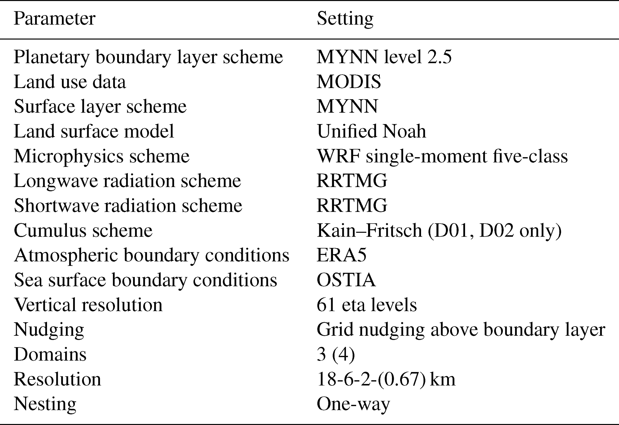
Figure 1a illustrates the one-way nested domains centered around the German Bight. One objective of this work is to assess the model sensitivity to the horizontal resolution. As such, simulations were carried out with either three nested domains, with the innermost domain having a resolution of 2 km, or an additional fourth nested domain with a resolution of 0.67 km. All wind turbines displayed in Fig. 1b were simulated from their commissioning date onward; hence simulations in earlier years contained fewer turbines. The colored turbines indicate the wind farms for which data were available in the study, while black turbines indicate the other simulated farms in the German and Danish waters of which no production data or information on operational state were available.

Figure 1 (a) Nested WRF domains centered around the German Bight, visualized using the WRF Domain Wizard tool (https://jiririchter.github.io/WRFDomainWizard, last access: 15 March 2024). (b) Simulated wind farms, with the studied farms indicated in color. The domain center and the floating lidars at TNW are also indicated.

2.1.2 Wind farm parameterizations

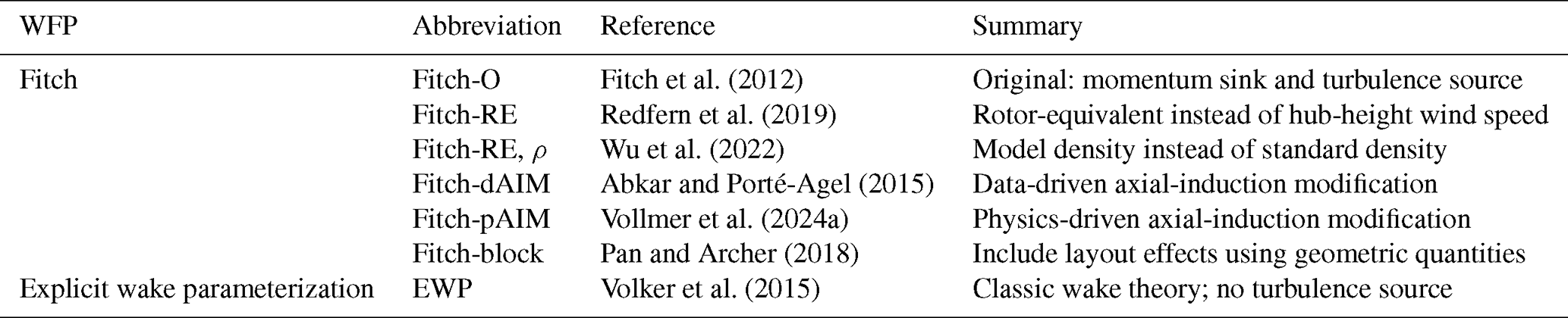
Seven wind farm parameterizations have been evaluated in this work. The implementation of five WFPs from Ali et al. (2022, 2023) was used, and two more WFPs (Fitch-RE, ρ and Fitch-pAIM) were added. All WFPs calculate the power and thrust coefficients by interpolating from prescribed look-up tables, which matched curves from installed turbines as closely as possible. Six of the WFPs are derived from the original Fitch parameterization, as can be seen from the overview in Table 2. EWP was also included, providing an alternative that includes an initial vertical wake expansion. A more detailed description of each WFP can be found in the introduction and Appendix A.

Fitch et al. (2012)Redfern et al. (2019)Wu et al. (2022)Abkar and Porté-Agel (2015)Vollmer et al. (2024a)Pan and Archer (2018)Volker et al. (2015)

Table 2 Overview of wind farm parameterizations, including reference papers and a short summary.

2.2 Validation data

2.2.1 Overview

SCADA data

The accuracy of the wind farm parameterizations was evaluated against SCADA (supervisory control and data acquisition) data from the wind farms' turbines. Details on six considered wind farms in the German Bight, indicated in Fig. 1b, are presented in Table 3. Since the Hohe See and Albatros wind farms are adjacent, they were considered to be one wind farm in this study. The length of the provided time period varied, as indicated in Fig. 2, but consisted of at least 2 years for each farm. SCADA data were provided by the wind farm operators at 10 min resolution at the wind turbine level. Only the wind speed from the nacelle anemometer, the wind direction from the nacelle wind vane, and the generated electrical power were used for analysis. Some additional variables were used for filtering and gap-filling the data, as explained in Sect. 2.2.2.

Figure 2 Data availability for the TNW floating lidars and the wind farms.

Table 3 Overview of six wind farms in the German Bight considered in this study.

Wind measurements

In addition to SCADA data, wind measurements from two profiling floating lidars at the TNW (Ten Noorden van de Waddeneilanden) site, indicated in Fig. 1b, were used. This measurement campaign, conducted between June 2019 and June 2021, was located west of the westernmost wind farm in the simulation domain. While this evaluation was based on a single point measurement within a domain of substantial spatial extent, hence where significant spatial variability is expected, the inclusion of these measurements was justified due to the large wind direction sector (including dominant wind directions) where the flow is undisturbed by wind farms. This enabled a meaningful, albeit limited, comparison between the model and observed data. The usage of other measurements closer to the studied wind farms in the period of interest was not possible as the offshore met masts FINO1 and FINO3 have both been surrounded by wind farms for several years, and the nacelle wind speed measurements from the SCADA data are too unreliable to be used for reference.

2.2.2 SCADA data processing

To ensure a fair comparison with the WRF results, the SCADA data were processed to derive a power time series at 10 min resolution, which is representative of 100 % turbine availability, hence eliminating non-normal operation like boosting, curtailment, and downtime.

Each turbine’s wind direction signal was compared with the wind direction average of the whole wind farm using weekly running averages. Sudden changes in the difference between an individual turbine and the farm average of more than 2° d⁻¹ were treated as discontinuities, for example due to sensor changes or resets. The offsets between these periods were then removed so that each turbine had a consistent wind direction signal over time. Even after removing discontinuities, the nacelle wind vanes may still have a constant angular offset relative to true north. To estimate this offset, wake losses from the SCADA data were compared with wake losses simulated using FOXES (Schmidt et al., 2023). An error in the wind direction measurement causes the observed wake loss pattern to appear rotated relative to the true compass directions. Therefore, the wind direction offset for each turbine was adjusted until the measured direction-dependent wake loss distribution matched the simulated one as closely as possible. Overall, the corrected mean absolute bias per turbine was approximately 3°, with 4 % of the turbines exceeding a 10° true north bias.

To flag curtailment and downtime, a polygon filter was used on the pairs of wind speed and power. Above a threshold wind speed slightly above rated wind speed, all power values below 98 % of rated power were flagged. Below this threshold, a box filter was applied in the mean pitch to mean power domain to exclude pitch angles that deviated by more than 1° from the pitch angles of regular operation. To derive the power estimate at 100 % turbine availability, a potential power was calculated for the flagged time stamps at each turbine, using the turbine power curves provided by the wind farm operators and a wind speed estimate at each turbine during downtime and curtailment. The wind speed estimate was calculated with a corrected 100 m reference wind speed from ERA5 (Hersbach et al., 2020). For the correction at every turbine a K-nearest neighbor (KNN) algorithm was used, trained during normal operation of the turbine and using wind direction at the turbine and month of the year as features, the latter as a proxy for atmospheric stability.

On average about 15 % of the power values were replaced with the estimated power. In below-rated conditions this decreases to 10 %. Because the gap-filling method represents the main source of uncertainty in the validation data, the uncertainty in the potential-power estimate was calculated using a Monte Carlo approach. Reference periods with more than 95 % of turbines in normal operation were selected. At randomly selected time stamps, the measured wind speed was replaced by the KNN-based wind speed estimate, and the resulting estimated power was compared with the measured power. The differences between both values were used to quantify the uncertainty associated with the potential-power estimate.

The uncertainty in the final energy yield estimate at 100 % turbine availability was calculated by multiplying the fraction of flagged periods by the average uncertainty in the potential-power estimate. For instance, an uncertainty of 10 % in the estimated power during 15 % of the time results in an overall uncertainty of 1.5 %. Across the wind farms considered in this study, the resulting wind-farm-level uncertainty due to the gap-filling procedure ranged from 0.1 % to 0.5 %. Individual wind farm uncertainties are not reported for confidentiality reasons.

Lastly, it should be noted that operational information from surrounding wind farms is not available and therefore cannot be accounted for. In particular, upstream wind farms that generate external wakes may at times be curtailed or experience downtime, which would reduce their wake impact on the wind farms investigated in this study. As a result, the SCADA power is likely slightly underestimated, an effect that is particularly relevant for the analysis of external wakes in Sect. 3.5.2.

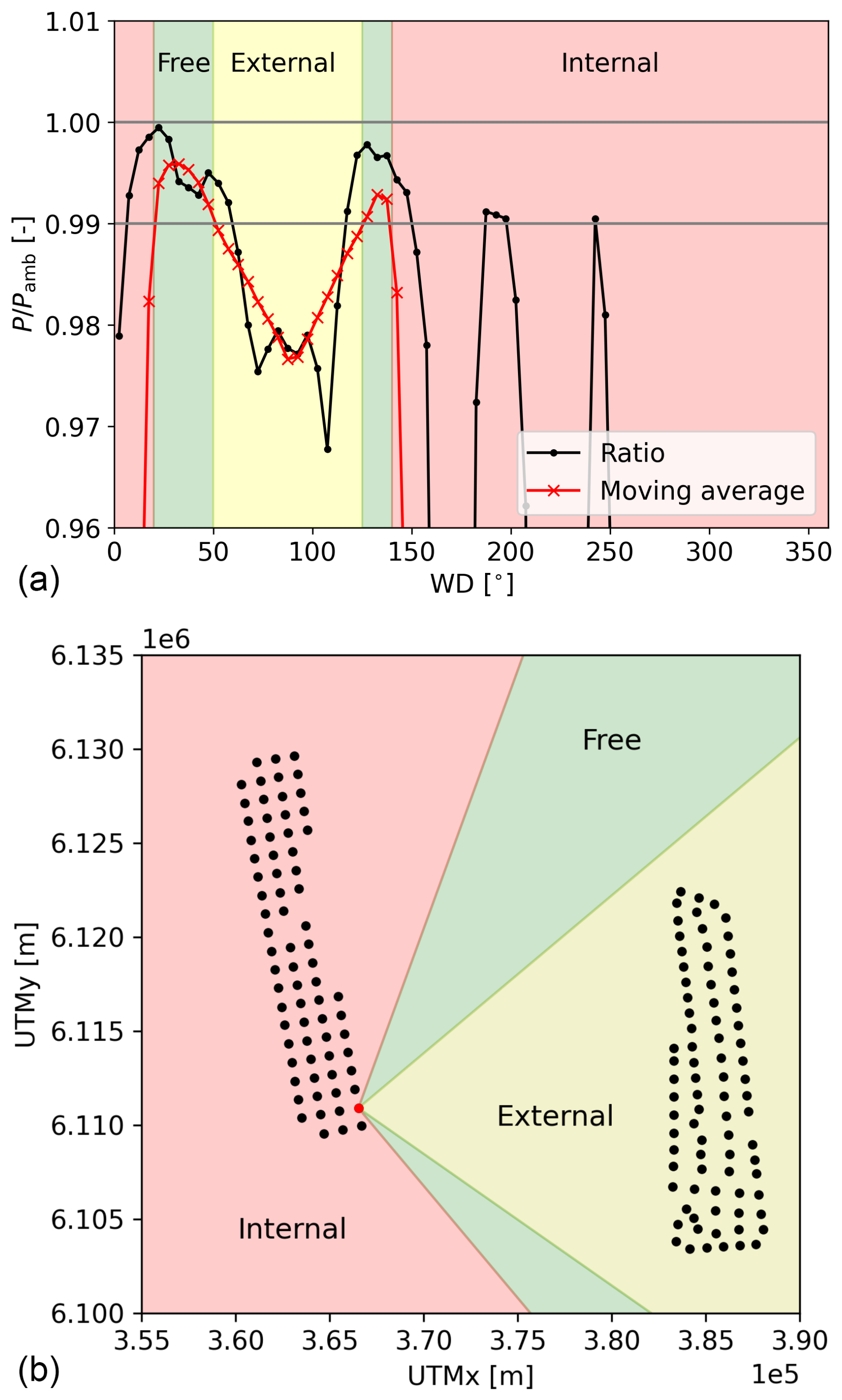
Figure 3 Illustrative example for identifying an undisturbed turbine using FOXES. (a) Ratio of generated power over ambient power (no wake losses) as a function of wind direction. (b) Spatial representation of undisturbed (free) wind direction sectors of the considered turbine indicated in red.

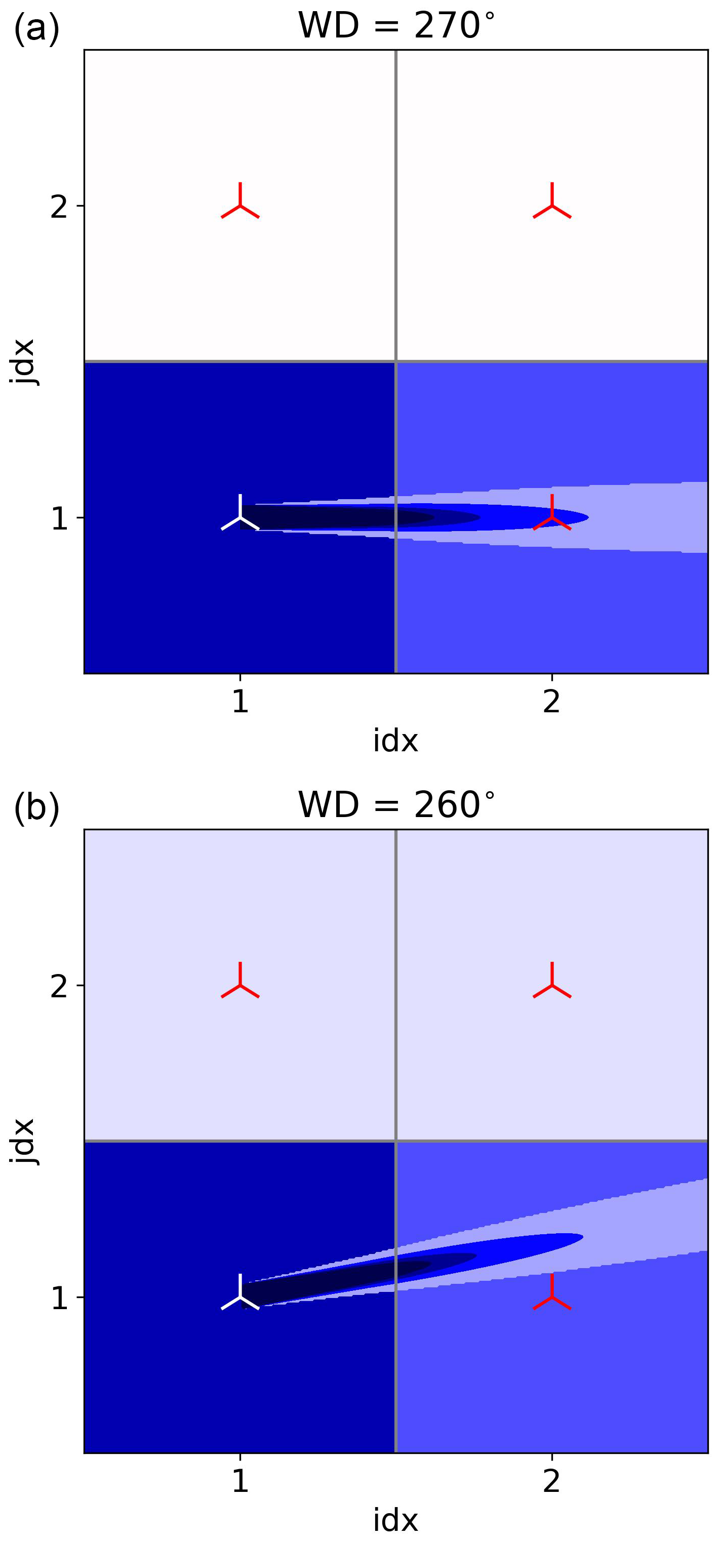
Figure 4 Sketch of transported momentum deficit (background color) for (a) WD = 270° and (b) WD = 260° of one wake-producing turbine (white) and three reference turbines (red). For comparison, the wake from FOXES is also included.

2.3 Identification of undisturbed turbines in model and measurement data

The analysis in Sect. 3.3 focuses on the reconstruction of the turbine's power curve from simulation results to verify whether the curves provided by the operators are used correctly by the different WFPs. To exclude the influence of wake effects, this analysis is restricted to undisturbed turbines. This section presents the method used to identify which turbines are undisturbed as a function of wind direction.

Wake simulations were performed using FOXES, yielding estimates of generated power and ambient power, which is derived directly from the background flow assuming no wake losses. Four-dimensional wind speed, wind direction, turbulent kinetic energy converted to turbulence intensity assuming isotropic turbulence, and the air density at the surface from the 4.5-year-long WRF simulation without turbines were passed to FOXES. All turbines in the domain were modeled in FOXES using the same specifications as in WRF.

Figure 3 illustrates the procedure for flagging a turbine as undisturbed using one turbine in the southeast of the Sandbank wind farm (marked red in Fig. 3b), which for certain wind directions is also waked by DanTysk. In Fig. 3a the ratio between the turbine's generated power and ambient power is shown (black line), together with a moving average (red line) over 45°. To flag a turbine as undisturbed in a certain wind direction, this ratio needs to exceed 0.99. In this example, the turbine is undisturbed in two narrow wind direction sectors and affected by either internal wakes or DanTysk's wind farm wake in the other sectors.

To ensure that turbines in WRF are undisturbed, an additional step related to the gridded nature of the simulations is needed. An example is illustrated in Fig. 4, where 2×2 WRF cells each containing one turbine are drawn. For the purpose of this illustration, only the white turbine in cell (1,1) is extracting momentum from the flow, while the other red turbines are passive observers. For a wind direction (WD) perpendicular to the grid orientation (Fig. 4a), the momentum extracted from the grid cell (background color) is passed to cell (2,1) directly downstream. Note that the magnitude of the wind speed deficit and the wake recovery are arbitrary and just for illustration purposes. At a slightly different wind direction (Fig. 4b), part of the extracted momentum is transported to cell (1,2). While the engineering model FOXES will flag this turbine as undisturbed (FOXES wake shown as reference), in the mesoscale model WRF this turbine will produce less power. For this reason, a turbine can only be considered undisturbed when at least two neighboring cells do not contain any turbines. For this example 2×2 wind farm, turbine (1,1) has undisturbed inflow for 180° < WD < 270° and turbine (1,2) for 270° < WD < 360°. The turbine in Fig. 3 does not experience any free inflow in WRF.

3 Results

3.1 Total energy yield

The total energy yield is computed as the sum over all turbines for the entire period during which SCADA data were available. Figure 5 presents this total energy yield from the simulations normalized with the SCADA energy yield at 100 % availability (Sect. 2.2.2). Both P_SCADA and P_WRF refer to electrical power, hence including electrical losses.

Figure 5 Total energy yield of the WFPs normalized by the energy yield at 100 % availability calculated from SCADA for each wind farm. Black bars represent the results at low resolution (2 km) and gray bars the results at high resolution (0.67 km). The shaded area around unity indicates the uncertainty in the SCADA (maximum of 0.5 %, as mentioned in Sect. 2.2.2).

The general trend is rather consistent between the wind farms. Fitch-O typically underestimates power by 3.1 % to 4.5 %. Modifications incorporating rotor-equivalent wind speed (RE) or the air density correction (ρ) yield minimal change. This reflects the offshore study area’s relatively low wind shear and the – on average – small difference to the standard air density. WFPs incorporating axial-induction modifications demonstrate the expected power increase. Fitch-dAIM continues to exhibit a power underestimation of several percent, whereas Fitch-pAIM generally overestimates power between 0.0 % and 4.1 %. Fitch-block shows a large underestimation of power, as it further decreases the power from Fitch-O by including internal wakes losses inside the grid cells. Other sub-grid-scale WFPs like the Jensen WFP (Ma et al., 2022a) have the same issue and are therefore not included in this work. Lastly, EWP consistently overestimates power, with deviations of between 0.0 % and 4.8 %.

Based on this analysis, to make the detailed analysis presented in the remainder of the paper more concise, only results from Fitch-O, Fitch-pAIM, and EWP are discussed as they represent the most fundamental differences between the WFPs.

To evaluate the sensitivity of the results to grid resolution, these three WFPs were run at a finer horizontal resolution of 0.67 km. The results of these simulations are presented on the right side of each panel of Fig. 5. All three models demonstrate an energy yield reduction compared to the coarser resolution, with Fitch-pAIM exhibiting the highest and EWP the lowest sensitivity to grid resolution.

While the total energy yield estimate remains the ultimate measure for a model's performance, it is a result of many factors, each contributing to the overall bias and uncertainty in the model. Therefore, the analysis in the following subsections attempts to look at the main sources of error individually. Those considered to have the greatest impact on the model result are the modeling of the wind speed (Sect. 3.2), the power curve (Sect. 3.3), internal losses (wakes and blockage; Sect. 3.4), and external wake losses (Sect. 3.5).

3.2 Wind speed

Figure 6a illustrates the Weibull distribution for the two floating lidars at the TNW site (TNW_A and TNW_B) and the corresponding grid points in both WRF domains (WRF_2 km and WRF_0.67 km) for free-inflow wind directions. The differences between the two lidars are negligible, as are those between the two WRF resolutions. The WRF distributions have a notable leftward shift compared to the measurement, corresponding to an average bias of approximately −0.25 m s⁻¹. Figure 6b furthermore demonstrates that this wind speed underestimation is consistent across wind directions, suggesting a systematic bias without clear directional dependencies. While this result cannot directly be transferred to the considered wind farms, it indicates that WRF most likely underestimates the wind speed at these sites. The observed underestimation falls well within the range of biases reported in the literature. For instance, Salvação and Guedes Soares (2018) examined locations off the Iberian coast and reported a mean annual wind speed bias over the open ocean ranging between −0.60 and −0.38 m s⁻¹ compared to satellite data. Closer to the shore, a comparison with buoy measurements indicated WRF biases of −0.07 to +0.59 m s⁻¹. Kalverla et al. (2019) analyzed 4 years of data from the IJmuiden met mast, located off the Dutch coast, and identified a bias of −0.25 m s⁻¹ at 27 m height and −0.5 m s⁻¹ at 115 m height. During the development of the New European Wind Atlas (NEWA), Hahmann et al. (2020) performed many sensitivity tests with different model configurations at several measurement sites. The model setup finally used to produce NEWA (Dörenkämper et al., 2020) was shown to have a mean wind speed bias of 0.21±0.51 m s⁻¹ against validation data in simple terrain. Lastly, Cheynet et al. (2025) demonstrated that compared to offshore and coastal measurements at around 150 m height, NEWA showed a wind speed bias between −0.82 and +0.49 m s⁻¹.

Figure 6 Comparison between measurements from two lidars (TNW_A and TNW_B) and WRF without turbines at 2 km and 0.67 km resolution. (a) Weibull distribution and annotated mean wind speed, (b) average wind speed per wind direction bin.

While the wind speed bias is relatively small, it has significant implications for subsequent power comparisons. To roughly estimate an energy yield bias from the wind speed distributions, the power curve of the generic NREL 5 MW turbine (Jonkman et al., 2009) was used. This exercise suggests an underestimation of the gross energy yield by WRF of around 3 %, which means that a correction would effectively shift the bars of simulated energy yield in Fig. 5 upwards.

3.3 Gross yield

The second source of error concerns the gross yield, evaluating whether the actual reconstructed power curves of individual turbines accurately reflect the theoretical power curves provided by the wind farm operators. This assessment could not be made for SCADA data as no undisturbed wind speed measurements were available. This section instead examines whether turbines modeled in WRF adhere to this prescribed curve correctly.

Figure 7 (a–c) Heatmaps of reconstructed power curve for one example wind farm for SCADA and three WFPs at 2 km resolution. The theoretical power curve is indicated with a solid red line. (d) Difference between reconstructed and theoretical power curve, normalized by the rated wind speed. Wind speed bins of 1 m s⁻¹ are used. Mean biases over all bins are indicated in the bottom left. All sub-figures: only undisturbed turbines are included, and the corresponding undisturbed wind speeds are obtained from a separate simulation without turbines.

Undisturbed turbines of only one wind farm were considered, as the other farms had very few undisturbed turbines in WRF. Turbines were flagged as undisturbed using the methodology outlined in Sect. 2.3. For each time step, the average wind speed and power output of all turbines flagged as undisturbed were considered, hence one value per time step. Figure 7a–c show heatmaps of this power curve reconstruction for one wind farm and the three WFPs, with the theoretical power curve displayed as a solid red line.

The results reveal a relatively high degree of scatter, arising from the decorrelation between the wind speed in a reference simulation without turbines (used here to determine the undisturbed wind speed) and the simulation with turbines (used for power). Among the WFPs, only Fitch-pAIM accurately reproduces the prescribed power curve. By contrast, Fitch-O and EWP display a systematic underestimation, a finding consistent with the results of Vollmer et al. (2024a) and the motivation behind the development of Fitch-pAIM described in this publication.

Figure 7d depicts the deviation of each reconstructed power curve (the wind speed binned mean of Fig. 7a-c) from the theoretical one, with the mean over all bins annotated in the bottom left corner. Fitch-O and EWP exhibit a noticeable underproduction, while Fitch-pAIM lies closest to the theoretical curve with a small underproduction. Interestingly, the finer resolution results in a significantly larger underestimation in Fitch-O and EWP. Just like the extracted momentum (wake effect), the turbine induction is also smeared out over the grid cell. The wind speed reduction due to induction, hence the difference between local grid cell wind speed and undisturbed wind speed, is therefore smaller for larger grid cells. When the local wind speed is used in power calculations, as done in Fitch-O and EWP, a turbine in a larger grid cell will produce more power. Fitch-pAIM does not have this limitation since it uses the induction-corrected free wind speed. Small deviations from the theoretical power curve and differences between resolutions for Fitch-pAIM are attributed to an imperfect correction function f (see Appendix A) or are hypothesized to be due to the global blockage effect.

While the power curve reconstruction analysis does not allow for a quantification of a bias compared to the measurements, it reveals that both Fitch-O and EWP have a systematic error in the power curve calculations. This results in a systematic negative bias in the gross energy yield estimate of the modeled wind farms.

3.4 Internal wake and blockage losses

This section discusses the uncertainties associated with internal wake and blockage losses. The focus here lies on wakes, averaged over all conditions (Sect. 3.4.1) and for specific wind directions (Sect. 3.4.2) and boundary layer heights (Sect. 3.4.3). Patterns of global blockage are analyzed in Sect. 3.4.4.

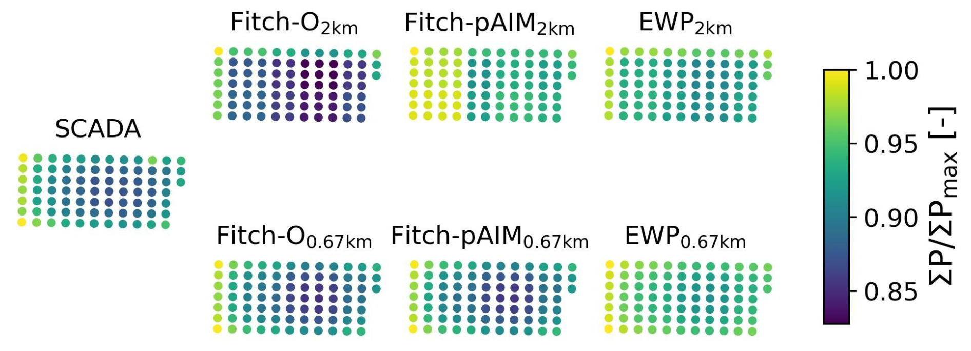
Figure 8 Amrumbank West patterns of production of total generated power per turbine, normalized by the maximum.

Figure 9 Scatterplots of total generated power per turbine, normalized by the maximum value in SCADA. Markers above the unity line indicate an overestimation of power by the model. Regression lines are fitted using orthogonal distance regression (ODR), and their slopes are annotated in the figures. To preserve confidentiality, the order of wind farms is arbitrary and differs from that in Fig. 5.

3.4.1 Mean power per turbine

Figure 8 displays the patterns of production (PoPs), the mean generated power per turbine over the whole time series (3 years) normalized by the maximum, for Amrumbank West. The SCADA PoP shows that turbines on the outer ring of the farm generate the most power as they receive undisturbed inflow at times. Higher values on the west side of the farm are due to the dominant westerly wind. Turbines in the center experience losses of up to 13 %.

At 2 km resolution, multiple turbines occupy one cell (up to nine; see Fig. B1b), indicated by identical colors. Compared to SCADA, Fitch-O displays systematically lower values, while EWP has higher values. At the finer resolution of 0.67 km, turbines do not share cells, and the patterns qualitatively match the SCADA PoP. Fitch-O again has a systematic underproduction; Fitch-pAIM shows a small underproduction, but the gradient over the farms seems accurate; and EWP displays an overproduction with a very small gradient, indicating small wake losses.

To quantify these results, scatterplots based on these PoPs are displayed in Fig. 9 for all wind farms. The average power from SCADA data is on the x axis and the WFP estimate on the y axis, meaning that values above the unity line indicate an overestimation of mean power by the model. The regression lines provide insight into the magnitude of the modeled wake deficit. Specifically, a regression line with a slope (indicated with annotated text) larger than unity indicates that the modeled wakes are stronger than those observed in the production data, whereas a slope smaller than unity suggests weaker modeled wakes.

At 2 km resolution, Fitch-O consistently underestimates power for all turbines across all farms (consistent with Fig. 5) and tends to slightly overestimate the wake effect. In contrast, EWP demonstrates significantly weaker wakes, resulting in a general overestimation of power. Fitch-pAIM shows the largest variability, having overly strong wakes in one farm, overly weak wakes in another one, and wakes of the appropriate magnitude in the remaining three farms.

At 0.67 km resolution, the power decreases across all WFPs. Consequently, the positive biases observed for Fitch-pAIM and EWP at 2 km diminish, while the negative biases for Fitch-O become more pronounced. The slopes of the regression lines change significantly with no clear trend between farms or parameterizations. Noteworthy is that the slope of Fitch-pAIM's regression line is close to that of Fitch-O, indicating that the slightly increased thrust due to the induction correction in Fitch-pAIM has only a small effect on the wake strength.

That EWP consistently shows an underestimation of the wake effect is likely due to the prescribed initial vertical expansion of the wake (see Appendix A), resulting in a higher hub-height wind speed used for power calculations.

3.4.2 Specific wind conditions

While the mean PoP is helpful to evaluate the WFPs' overall representation of internal wakes, responses to specific atmospheric conditions vanish due to averaging. To better understand the models' sensitivities, this section focuses on narrower wind direction sectors and wind speeds (WSs) below rated (6 m s⁻¹ < WS < 10 m s⁻¹).

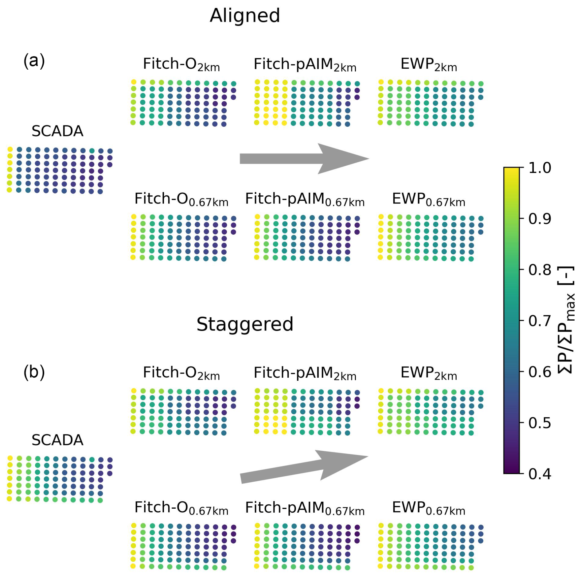
Figure 10 Patterns of production for Amrumbank West for 6 m s⁻¹ < WS < 10 m s⁻¹ for (a) aligned conditions $\mathrm{267.5}\mathit{°}<\mathrm{WD}<\mathrm{272.5}\mathit{°}$ and (b) staggered conditions $\mathrm{257.5}\mathit{°}<\mathrm{WD}<\mathrm{262.5}\mathrm{°}$.

Figure 10 shows PoPs for Amrumbank West, filtered for wind speeds below rated and one wind direction in which the turbines are aligned (Fig. 10a) and one in which they are staggered (Fig. 10b). In the aligned condition, SCADA illustrates a huge drop in power from the first to second row, which is not reproduced by any WFP at any resolution. The coarse resolution shows big step-wise power reductions between cells, whereas this is more gradual at finer resolution. In staggered conditions, the fine-resolution simulations are able to accurately reproduce the pattern observed in SCADA apart from systematic biases, while at the coarse resolution the model results clearly show the effect of multiple turbines in a cell.

Figure 11 Single-row analysis for Amrumbank West (a–c) and Sandbank (d–f) for 6 m s⁻¹ < WS < 10 m s⁻¹. Farm layouts are indicated in (a) and (d), with the studied turbines in red markers, the aligned wind direction ($\mathrm{267.5}\mathrm{°}<\mathrm{WD}<\mathrm{272.5}\mathrm{°}$ for Amrumbank West and $\mathrm{167.5}\mathit{°}<\mathrm{WD}<\mathrm{172.5}\mathit{°}$ for Sandbank) with a solid gray line, and the staggered wind direction ($\mathrm{257.5}\mathit{°}<\mathrm{WD}<\mathrm{262.5}\mathit{°}$ for Amrumbank West and $\mathrm{177.5}\mathit{°}<\mathrm{WD}<\mathrm{182.5}\mathit{°}$ for Sandbank) with a dashed gray line. The power of each turbine, normalized by the front-row turbine, is displayed for aligned conditions (b, e) and for staggered conditions (c, f).

To highlight these findings further, Fig. 11 focuses on single rows of turbines in Amrumbank West (top) and Sandbank (bottom). The farm layout, the selected turbine row, and the two wind directions under consideration (aligned and staggered) are illustrated in Fig. 11a, d. The other figures display each turbine's power, normalized by the power of the front-row turbine.

For aligned cases (Fig. 11b, e), a substantial drop in power from the first to the second turbine is visible in SCADA. The WFPs show a more gradual power reduction over the first few turbines. Clearly visible from their identical power is that several grid cells contain multiple turbines in the 2 km simulation. The power output of downstream turbines tends to level out in the measurements, which has been mentioned in the literature (e.g., Hancock, 2013; Bay et al., 2023). However, in the WRF simulations, the power output continues to decrease along the row, which is particularly visible for the simulations at 0.67 km. In the aligned cases (Fig. 11c, f), the measurements exhibit a more gradual reduction in power with downstream distance. Especially visible at 0.67 km, there is a systematic difference between EWP and the others, with Fitch-O and Fitch-pAIM being more accurate at Amrumbank West and EWP at Sandbank.

The thrust applied by the turbines is smeared over the whole grid cell as already shown in Fig. 4, explaining the model's inability to represent the large drop in power at the second turbine. Modeled power values are actually almost the same in the aligned and the staggered cases, as a wind direction difference of ΔWD = 10° changes the wind speed deficit in a downstream grid cell by $\mathrm{1}-\cos \mathrm{\Delta }\mathrm{WD}=\mathrm{1.5}\mathit{\%}$. For this reason, it cannot be expected from the mesoscale model to replicate the measurements for such a narrow wind direction sector. This indicates that aiming to reduce the difference between measurements and models only for aligned conditions is not recommended.

A few other findings are noteworthy. The results for Fitch-pAIM at 2 km (Fig. 11b) show an unexpected pattern, as the power for turbines 2–4 is higher than for the first turbine. This suggests that the assumption underlying Eq. (A16), that the induction factors of all turbines in a grid cell can be multiplied to correct the wind speed of the grid cell, does not hold universally. In Fig. 11e, f at 2 km resolution, the second turbine has the same power as the front-row turbine as they are placed in the same grid cell (Fig. B1a), which consequently results in a very large deviation from the measurements in aligned conditions. This explains why generated power decreases with increased resolution, as already observed in Fig. 5. At 0.67 km, the second turbine experiences a lower wind speed than at 2 km, leading to reduced power. This extends to all turbines that share a grid cell with others, resulting in a significant reduction in generated power as the horizontal resolution of the simulation increases.

Figure 12 Power ratios between two turbines at Amrumbank West (a) and Sandbank (b) indicated by big red markers in Fig. 11a, d for a range of wind directions and 6 m s⁻¹ < WS < 10 m s⁻¹.

Next, a side-by-side comparison between two turbines, one undisturbed and one waked separated by several turbines, is presented. It should be noted that the power of the undisturbed turbine in the model used as a reference is not constant. It is affected by a change in resolution, as the induction is also smeared out over the whole grid cell (Fig. 7). Additionally, the wind speed deficit coming from neighboring cells affects the wind speed of the cell of the reference turbine (Fig. 4), the magnitude of which is dependent on the wind direction. The results shown here should therefore be considered qualitatively only.

Figure 12a looks at two turbines in the same row in Amrumbank West as in Fig. 11a, indicated by the larger red markers. It shows a steadily increasing power ratio (smaller wake losses) across wind direction bins from 230 to 310° due to fewer upstream turbines. This change is rather gradual in both measurements and WFPs, with the exception of WD = 270°, where the turbines are aligned. Here again the measurements show a significantly larger wake loss, which is not reproduced by any of the simulations. Apart from consistent biases, both resolutions show the same pattern of result. EWP again models the weakest wakes, but it is interesting to note that at 2 km Fitch-O has the lowest power ratio, whereas at 0.67 km this is Fitch-pAIM. The higher thrust force in Fitch-pAIM due to the axial-induction-corrected wind speed leads to stronger wakes, resulting in a lower power ratio than Fitch-O at 0.67 km. At 2 km, however, this effect is outweighed by the issue of multiple turbines in one cell, which amplifies the induction correction more for T6 (in a cell containing six turbines; see Fig. B1b) than for T2 (in a cell containing three turbines), resulting in a higher power ratio than Fitch-O.

At Sandbank (Fig. 12b) the SCADA data display a pattern symmetrical around the aligned condition at WD = 170°, where wake losses are significantly larger than at other wind directions. This again is not reproduced by the WFPs, which show an asymmetry with larger losses for WD > 170°. This is directly related to the larger number of turbines in the southwest corner of the farm compared to the southeast corner. The differences between WFPs and resolutions are similar to Fig. 12a.

The side-by-side analysis clearly further illustrates that mesoscale models are not able to capture the magnitude of wake effects when turbines are aligned but might overestimate the wake effect when turbines are staggered.

3.4.3 Sensitivity to the vertical structure of the atmosphere

This section investigates how the wake magnitude is affected by the vertical structure of the atmosphere. The planetary boundary layer height (h_BL) from the WRF model output was selected as a filter metric, an alternative to a stability metric. It was chosen instead of the Obukhov length as it better reflects the conditions affecting the wake recovery. Uncertainties associated with WRF's h_BL estimates should be considered; hence the classification in this section is intended for qualitative interpretation only. Three discrete classes were considered, separated by the 33.3rd and 66.7th percentiles (following Baas et al., 2023) of the h_BL in the results of the WRF simulation without turbines after filtering for the wind speed and direction considered here: low (h_BL < 616 m), mid (616 m < h_BL < 943 m), and high (h_BL > 943 m) boundary layers. The same WRF h_BL was also used to bin the SCADA data in the absence of a measurement, introducing some uncertainty. Focus of the analysis was to reproduce Fig. 11c, hence a single-row analysis at staggered conditions in Amrumbank West under different h_BL. For brevity, only results from the finer-resolution simulations are included.

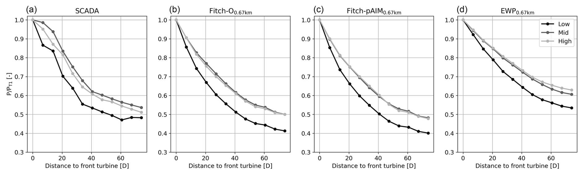
Figure 13 Effect of boundary layer height on the power deficit of a single row of turbines in Amrumbank West for $\mathrm{257.5}\mathit{°}<\mathrm{WD}<\mathrm{262.5}\mathit{°}$ and 6 m s⁻¹ < WS < 10 m s⁻¹, hence corresponding to Fig. 11c. Classes are low (h_BL < 616 m), mid (616 m < h_BL < 943 m), and high (h_BL > 943 m).

The results in Fig. 13 illustrate that the difference between mid and high boundary layers is small in the SCADA data but that in low boundary layers the power deficit is about 20 % larger. This is physically sound, as low boundary layer heights are related to more stable conditions in which less mixing takes place, and the vertical turbulent transport of momentum is reduced by the presence of the temperature inversion that caps the boundary layer. This dependency is rather well reproduced in WRF, where especially in Fitch-O and Fitch-pAIM the magnitude of the deficit is similar, and no large difference between mid and high boundary layers is observed. In EWP the deficits are consistently smaller, and there is a substantial difference between mid and high boundary layers. It is hypothesized that this is due to the initial smearing of the extracted momentum, as explained in Appendix A.

These results indicate that WRF is well able to capture the physics associated with wake recovery under different atmospheric conditions.

3.4.4 Global blockage

A direct quantification of global blockage is not possible by only using production data from a wind farm, as the pressure-driven global blockage effect modifies the wind resource that is available to the wind farm compared to the hypothetical situation in which there would be no wind farm. It also leads to a redistribution of momentum from front-row wind turbines to turbines deeper inside the farm (Lanzilao and Meyers, 2022; Centurelli et al., 2024), an effect that cannot be distilled from the data. Rodaway et al. (2024) revealed the existence of global blockage by looking at the average power of the northernmost turbines of Amrumbank West for slight deviations of the wind direction. This analysis was not possible with the mesoscale model, as these turbines can only be considered undisturbed for wind directions perpendicular to the grid orientation (as discussed in Sect. 2.3). Instead, this section addresses the existence of blockage by showing the deceleration of wind speed from the simulations upwind of the farm. The focus in Fig. 14 is on Amrumbank West due to its favorable orientation to study blockage for westerly flow (WD ≈ 270°). The spatial plots, illustrating the wake deficit at 100 m of Fitch-pAIM relative to the simulation without turbines, clearly depict the wake deficit, as well as the Kaskasi gap between the wind farms. However, the focus here lies on the cells located immediately upstream of the first row of turbines. For both resolutions, it can be observed that the first cell upstream has a lower wind speed than cells further upstream. Figure 14c illustrates the wind speed reduction as a function of upstream distance along the cross-section indicated by the solid red lines, where x=0 km denotes the center of the cell containing the first turbine. At 2 km, the wind speed reduction one cell upstream is slightly greater than two cells upstream. At 0.67 km, a more gradual decrease in wind speed extending multiple upstream grid cells is visible, while the magnitude is similar to that at 2 km. Approximately 10 km upstream of the wind farm, the wind speed deficit is still around 1 %. This reduction is not due to global blockage, but rather to the external wakes originating from wind farms located 50 km to the west (Hohe See, Albatros, and Global Tech I; see Fig. 1b).

The physical accuracy of these observations requires further validation, which is considered beyond the scope of the current work. However, it is noteworthy that the mesoscale model captures any wind speed reduction upstream of the wind farm, a signature of global blockage. In the evaluation of the wind farm parameterizations, it can be considered another source of error.

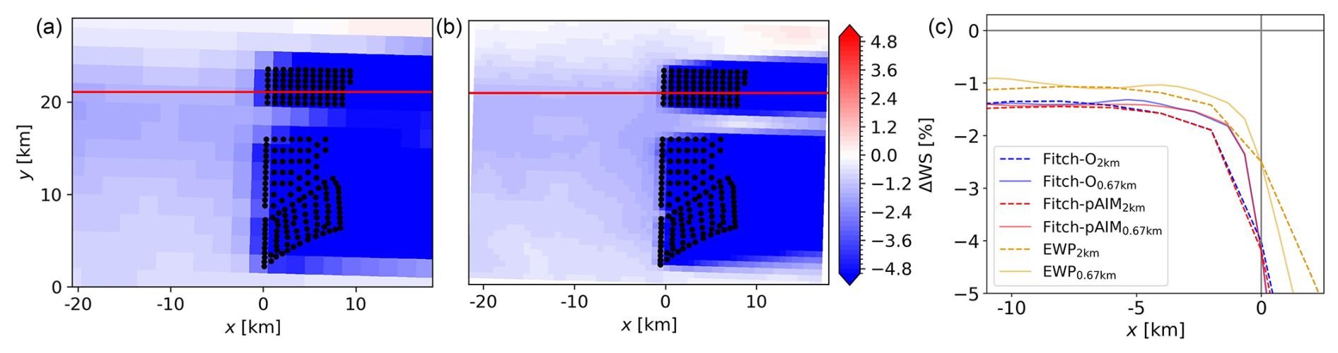
Figure 14 The effect of blockage on wind speed at Amrumbank West. Spatial plots of the wind deficit at 2 km (a) and 0.67 km (b) for Fitch-pAIM relative to the WRF simulation without turbines. (c) Wind speed deficits of all WFPs and resolutions as a function of upstream distance along the solid red lines. All data filtered for 267.5° < WD < 272.5°.

3.5 External wake losses

This section evaluates how well external wakes (i.e., cluster wakes or wind farm wakes) are modeled by the WFPs. Section 3.5.1 studies the wind field between clusters, after which Sect. 3.5.2 investigates the effect on the power of front-row turbines of a downstream wind farm. As an illustrative example, the external wake effect on the Hohe See and Albatros wind farms is shown, while similar phenomena are expected to occur at other wind farms in the studied domain. It should be noted that a direct translation of these results into economic or contractual performance indicators of individual wind farms would not be appropriate without further dedicated analysis.

3.5.1 Wind speed

This section analyzes the wind speed between upstream of Hohe See and Albatros. Validation of these results was not possible due to a lack of observational data; hence no lidar or flight data were available. Figure 15a–b illustrate the wind speed deficit modeled with Fitch-pAIM relative to a simulation without any turbines, at 100 m for a wind direction of 235° and all wind speeds. The difference in spatial resolution is clear from the granularity of these plots, but the magnitude of the wind speed deficit appears consistent across resolutions.

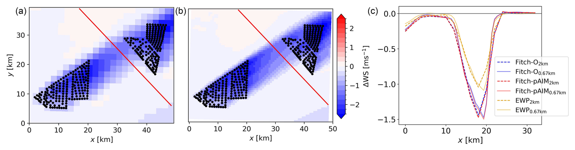
Figure 15 Wind speed deficit affecting Hohe See and Albatros at 2 km (a) and 0.67 km (b) resolution. (c) Wind speed deficits along the cross-section indicated by the red line in the spatial figures, taken from bottom right to top left. All data filtered for 232.5° < WD < 237.5°.

Figure 15c presents the wind speed deficit along the solid red line, reaching up to 1.5 m s⁻¹. Among the models, EWP exhibits again the weakest wake effects, while both Fitch-O and Fitch-pAIM display comparable deficits, with the latter showing a slightly more pronounced wind speed reduction due to increased thrust from the induction correction. This represents an average between a thrust force increase below and a decrease above rated wind speeds, weighted by the wind speed distribution. The resolution does not appear to have a significant impact on the magnitude of the wake deficit. What can be seen is a slight shift in the location of the maximum deficit and a larger gradient at the edge of the cluster wake, both due to the difference in grid resolution.

As far as comparisons to the existing literature allow, these results align well with previous findings. In a study focusing on several months of scanning lidar wind measurements in a wind farm cluster, Cañadillas et al. (2022) demonstrated strong agreement between simulated cluster wakes from Fitch-O and lidar data, although a slight underestimation of the wake effect was observed. Similarly, in a comparison with FINO-1 data and airborne measurements, Ali et al. (2023) found that Fitch-O generally captured the wind speed reductions under cluster wake conditions well, albeit also with a slight underestimation of the wake effect. Also in this work, EWP exhibited a much larger overestimation of wind speed in the wake.

3.5.2 Turbine power

This section focuses on the effect of the external wakes on the power ratio of front-row turbines, averaged over three on the northern and three on the southern side, which has the same implication as discussed in Fig. 12. The turbines, indicated in Fig. 16a, were carefully selected, accounting for the effect discussed in Fig. 4, ensuring no influence from turbines in neighboring cells. For this reason, only results for 0.67 km are shown. In contrast to Sect. 3.4.2, no wind speed filter was applied as deriving an undisturbed wind speed was not possible due to the external wake effect, so a wind speed bias between SCADA and model results cannot be excluded. By sweeping over wind direction sectors, conditions could be analyzed where either the northern three or southern three turbines are affected by the external wake.

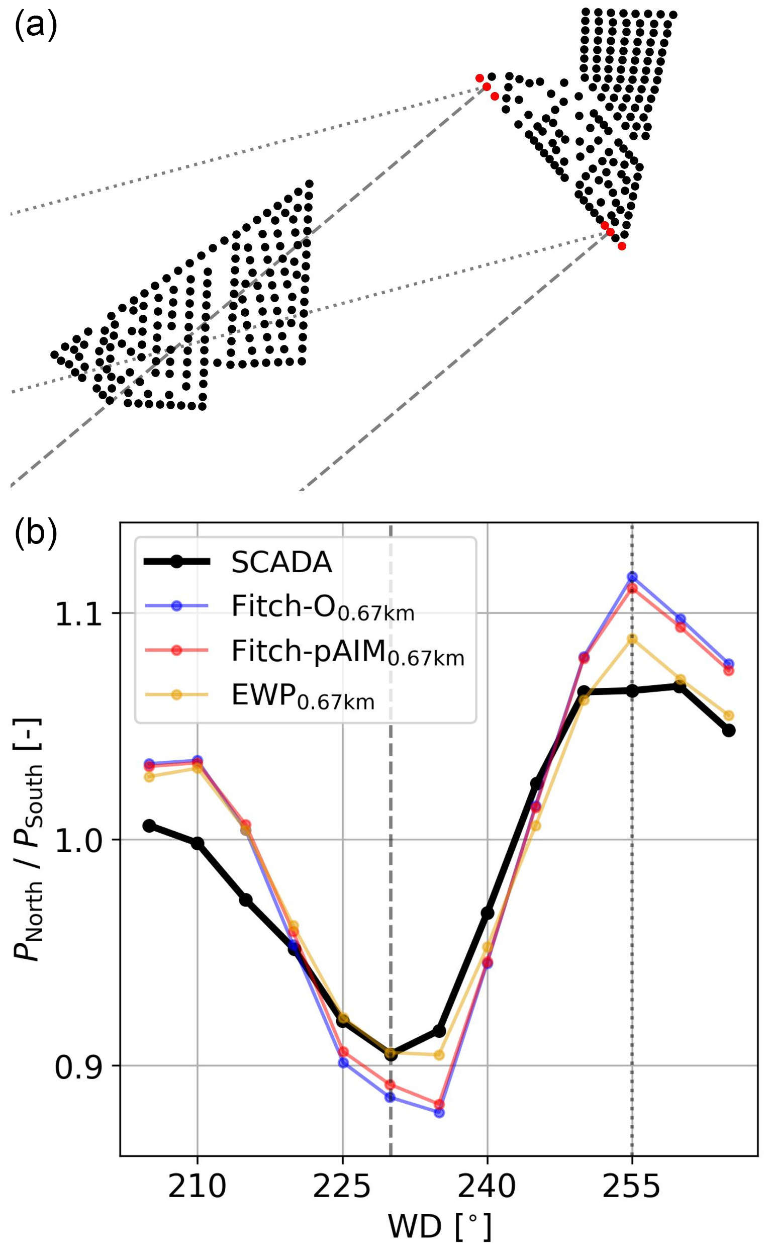
Figure 16 (a) Farm layout with the studied front-row turbines as red markers. (b) Power ratio between the northern and southern turbines affected by a cluster wake for a range of wind directions. Two wind directions representing roughly the largest power losses are indicated by the dashed and dotted gray lines.

The wake reaching the Hohe See and Albatros wind farms (Fig. 16b) causes a measurable but moderate reduction in power output at the selected front-row turbines. The magnitude of these effects is generally within the single-digit to low-double-digit percentage range, depending on wind direction and with that the distance to the upstream wind farm. WRF does reproduce this asymmetry, with differences between the WFPs being small. EWP again produces the weakest wakes, which here provide the best agreement with the SCADA data, while Fitch-O and Fitch-pAIM tend to overestimate the wake losses. However, it should be noted that upstream wind farms are experiencing curtailment and downtime, which could not be accounted for in this analysis. As a result, the wake losses indicated by the SCADA data are likely slightly underestimated. Interestingly, Fitch-O has slightly higher wake losses than Fitch-pAIM, which is opposite to the wind speed deficit observed in Fig. 15c. This is due to the mean wind speed at the turbines, which is lower for the waked turbine and therefore likely in the steepest part of the power curve. A small axial-induction correction of the wind speed in Fitch-pAIM therefore increases the power of the waked turbine more than the power of the undisturbed one, resulting in slightly smaller losses when looking at the power ratio.

While these findings should be interpreted qualitatively only, they strengthen the findings of Sanchez Gomez et al. (2024) that WRF is well able to capture the external wake effect, and with minimal differences between the parameterizations. This also makes sense when considering that the further downstream a wake propagates, the more its evolution is controlled by boundary layer processes rather than the WFP. Since the same planetary boundary layer (PBL) scheme is used in all simulations, differences in the wake deficits close to the farm generated by the WFPs are smoothed during downstream propagation and therefore have a reduced influence on the external wake.

4 Discussion

This section discusses the constraints under which this study was carried out and therefore aspects that must be considered when interpreting the presented results.

The aspects mentioned in this section are expected to affect the results. However, the general findings of this work are likely to remain valid:

• All WFPs except for Fitch-pAIM will systematically underestimate power at undisturbed turbines because they calculate power from the locally reduced grid cell wind speed rather than from the induction-corrected free-stream wind speed used in the power curve.

• EWP continues to generate substantially weaker wakes compared to Fitch-O and Fitch-pAIM due to its prescribed initial vertical expansion of the wake resulting in higher wind speeds at hub height used for power and thrust calculation at downstream turbines.

• External wakes are similar for all WFPs because their downstream evolution is governed by the physics of the common PBL scheme.

4.1 Wind speed bias

Different choices in the model setup (e.g., physics schemes, dynamics, and global model forcing) lead to significant differences in the wind speed estimates, as shown in the sensitivity studies carried out in Hahmann et al. (2020). This study used a setup tailored to the area of interest and therefore had a relatively small mean wind speed bias of 0.25 m s⁻¹ at the TNW lidar location (Sect. 3.2), leading to a power difference of around 3 % for a 5 MW turbine. Note that this analysis excluded easterly wind and only evaluates a single point, while substantial variability could occur in the domain.

While many studies get around this bias by evaluating wake losses instead, this requires a reliable estimate of the undisturbed wind speed, which in this study was not possible to obtain for the SCADA data due to the many wake-generating wind farms.

Considering the wind speed bias, it is argued that the total power bias shown in Sect. 3.1 is not a valid metric to assess which wind farm parameterization is most accurate. While it is an attractive metric due to is simplicity, results are highly dependent on the wind speed distribution, and the “best”-performing WFP can simply be due to errors canceling out. These results do allow for a comparison between WFPs, as the simulated background wind speed is the same.

The rest of the study attempted to assess the performance of the WFPs by taking wind speed difference out of consideration.

4.2 Wind farm parameterizations

Some consideration related to the modeled turbines should be mentioned. Firstly, in Fig. 5, it was shown that modification incorporating the rotor-equivalent wind speed and air density yielded minimal change, reflecting the offshore study area. It should be noted that at higher altitudes, these corrections are expected to have a larger impact, as shown in Chang et al. (2026).

Secondly, Mangara et al. (2019) illustrated that the number of vertical model levels inside the rotor area affects the wind speed deficit in the wake. Future work should study in more detail how aspects related to the wind farm parameterizations (momentum extraction and turbulence generation) and aspects related to the boundary layer schemes (wake recovery, turbulence dissipation) are affected.

Thirdly, the distribution of turbines over cells affects the generated power, especially at coarser resolution, where turbines share cells. This is best illustrated by Fig. 11e, f, where at 2 km resolution the first two turbines share a cell and receive undisturbed wind. If these turbines were split between cells, the second turbine would generate less power. However, at the level of a full wind farm over a longer time, this issue is expected to have a smaller effect than the spread between models.

Lastly, all wind farm parameterizations rely on at least one empirical (tuning) or correction factor, as can be seen from their equations in Appendix A. In this study, only default or recommended values were used, but calibrated values are expected to have a significant impact on the results. More details are discussed below.

Most Fitch-related WFPs use a correction factor for the TKE coefficient. Its default value of α_TKE=0.25 was proposed by Archer et al. (2020), based on a small study comparing the turbine-generated TKE from Fitch with that of a single LES run containing one turbine in a neutral boundary layer at a wind speed of 9 m s⁻¹. While this factor barely affects the wind speed deficit in the cell in which the turbine is located, Ali et al. (2023) demonstrated it does influence the wake recovery and therefore the power of downstream turbines. Recent work by Sengers et al. (2026) proposed a new analytical equation derived from the 1D momentum theory to compute the TKE coefficient, making this correction factor obsolete. Using this new equation, slightly more TKE is added to the flow than when using α_TKE=0.25, resulting in a small power increase due to faster wake recovery.

Fitch-dAIM contains a correction factor that varies depending on wind farm configuration and needs to be tuned to a higher-fidelity data set varying wind speed and direction. While the accuracy of a fully calibrated Fitch-dAIM is expected to be high, generating a reference data set for the full German Bight is computationally not feasible.

Fitch-block uses geometric quantities and a multiple linear regression function fitted to results from five LES runs of one wind farm at neutral stratification to define a correction function used in the tendency and power equations. Additionally it assumes that the maximum wake recovery distance is 20 D, although wind farm wakes are especially known to last longer. While Fitch-block was designed to reduce power compared to Fitch-O for aligned turbines, most of the time turbines are staggered, and simulated power is often underestimated. Since Fitch-block does not correct for this, Fitch-O can be considered its upper limit, which results in a large underestimation of power compared to production data. This is also the reason why other sub-grid-scale parameterizations like Jensen (Ma et al., 2022a) were not included in this study, as these have the same limitations. EWP relies on an initial length scale ${\mathit{\sigma }}_o=\frac{\mathrm{1}}{\mathrm{2}}\cdot {\mathit{\sigma }}_R\cdot D$ for the vertical wake expansion. Here, σ_R is an empirical parameter whose default value was tuned to measurements of a 2 MW turbine. It is however unknown how this value changes for other turbine types of different sizes and rated power, with the authors (Volker et al., 2015) noting that measurements of other turbines are needed to reassess its value.

4.3 Generalizability

Although this study considered data from six offshore wind farms situated in the German Bight, the geographical concentration raises the question of applicability to other regions. Provided that biases in wind speed distribution are similar, it is expected that the outcomes are transferable to other offshore sites globally. Many other regions employ lower turbine densities, so the criterion of one turbine per cell will be achieved at a coarser resolution. However, onshore environments are characterized by higher turbulence intensities and larger variability in atmospheric stability, which might not have been included in the current study. Furthermore, a more complex topography makes the vertical representation of the wake more relevant.

Planned and future wind farms will consist of many more turbines and larger turbines than the wind farms considered in this study. The accuracy of existing wind farm parameterizations on these scales is unknown. However, the absolute spacing between turbines will increase, so the criterion of one turbine per cell will be achieved at a coarser resolution.

Lastly, when other mesoscale models or other planetary boundary layer schemes (coupling with WFPs currently not available in the official WRF release) are used, the wake recovery rate could be affected, thereby constraining the transferability of the presented results.

4.4 Implications for applications

The results provide several practical implications for the use of mesoscale models and their wind farm parameterizations in wind resource assessments. Firstly, a sufficiently fine horizontal resolution that limits the number of turbines within the same grid cell is highly recommended. Secondly, the choice of WFP affects the power estimates substantially, with Fitch-pAIM shown to provide the most consistent representation of undisturbed turbine power and average wake losses. Lastly, unavoidable biases in the background wind speed, as well as the impact of model choices on the results, should be carefully considered when absolute energy yield is of interest.

Mesoscale models are less suitable than engineering wake models for applications that depend on detailed turbine interactions, such as layout optimization or analyses of narrow wind direction sectors. However, their performance improves when considering broader wind direction ranges and therefore appear well suited for wind-farm-scale AEP assessments, provided that the AEP is not dominated by only a few narrow wind direction sectors. Their strength lies in the representation of interactions between wind farms and the atmosphere, something that is lacking in engineering wake models, making them particularly useful for assessing future wind farm build-out scenarios.

In general, the presented results support applications based on longer-term-averaged quantities, while phenomena on the short timescale, and therefore turbine scale, remain insufficiently resolved. This makes mesoscale models with WFPs complementary to, rather than a replacement for, engineering and higher-fidelity wake models.

5 Conclusions

This study assessed the accuracy of seven existing wind farm parameterizations (WFPs) within the WRF model by a comparison with SCADA data from six offshore wind farms in the German Bight. Fitch modifications integrating air density and rotor-equivalent wind speed showed a negligible influence on power production in the studied offshore region. The use of a sub-grid-scale model to capture layout effects led to substantial underestimation of power, while an uncalibrated, data-driven axial-induction modification failed to demonstrate the expected improvements. A more detailed evaluation at spatial resolutions of 2 and 0.67 km was conducted for the three remaining parameterizations: the original Fitch scheme (Fitch-O), Fitch incorporating a physics-derived axial-induction modification (Fitch-pAIM), and the explicit wake parameterization (EWP). The main results of the following are summarized in Table 4.

Table 4 Qualitative summary of the main results. Downward and upward arrows indicate underestimation and overestimation of generated power as a result of these sources of error, double arrows indicate a stronger bias, and circles indicate no substantial bias.

Total energy yield estimates showed large variability between WFPs, but results were consistent between farms with Fitch-O underestimating and Fitch-pAIM and EWP overestimating power. With increasing resolution the estimated power decreased, attributable to a reduced number of turbines per grid cell and therefore enhanced internal wake effects. The main sources of error were addressed in the remainder of the work.

An underestimation of 0.25 m s⁻¹ of the mean wind speed, leading to an AEP difference of about 3 %, was found compared to lidar data. While not generalizable to the locations of the considered wind farms due to variability in the simulation domain, this result suggested a systematic underestimation of the energy yield by a few percent. Reconstruction of the power curve for undisturbed turbines revealed that only Fitch-pAIM approached the theoretical power curve, whereas both Fitch-O and EWP displayed a systematic underestimation of gross energy yield with a dependency on the grid resolution. Internal wakes were underestimated for aligned turbine configurations, whereas they tended to be overestimated in staggered conditions. Given that the spatial resolution of WRF restricts accurate representation of internal wakes in narrow wind direction sectors, power estimates should be evaluated only over broader wind direction sectors to ensure robustness. At finer resolution, both Fitch-O and Fitch-pAIM yielded accurate representations of average internal wake magnitudes. At the coarser resolution the variability between wind farms was considerable, limiting the generalizability of the results. What is consistent is that EWP underestimated the internal wake effect across all resolutions and sites. Lastly, the magnitude of external wakes was well captured by all WFPs across all resolutions.

The presented results should be interpreted with care due to the associated sources of error, including deviations in mean wind speed, model configuration, and SCADA data uncertainty. Additionally, the applicability of the results for larger wind farms and future turbines is unclear. Nevertheless, this study is believed to demonstrate that, at a resolution fine enough to allocate individual turbines to separate grid cells, the Fitch-pAIM wind farm parameterization achieves the highest level of accuracy.

Appendix A: Wind farm parameterization equations

A1 Fitch et al. (2012): original fitch parameterization (Fitch-O)

The original Fitch parameterization calculates the turbine's thrust and induced turbulent kinetic energy (TKE) that affect the flow using the following equations:

$$\begin{array}{}\text{(A1)}& {\displaystyle }& {\displaystyle \frac{\partial u_k}{\partial t}}=-{\displaystyle \frac{\mathrm{1}}{\mathrm{2}}}\cdot C_{\mathrm{T}}\left(U_{\mathrm{h}}\right)\cdot u_k\cdot U_k\cdot A_{\mathrm{rot},k}\text{(A2)}& {\displaystyle }& {\displaystyle \frac{\partial {\mathrm{TKE}}_k}{\partial t}}={\displaystyle \frac{\mathrm{1}}{\mathrm{2}}}{\mathit{\alpha }}_{\mathrm{TKE}}\cdot \left(C_{\mathrm{T}}\right(U_{\mathrm{h}})-C_{\mathrm{P}}(U_{\mathrm{h}}\left)\right)\cdot U_k^{\mathrm{3}}\cdot A_{\mathrm{rot},k},\end{array}$$

in which subscript k indicates the vertical level, subscript h hub height, U the horizontal wind speed, and u its component along the x axis. The momentum equation for the v component is analogous to Eq. (A1) but omitted here for brevity. A_rot,k is the area occupied by the turbine rotor between two vertical model levels, resulting in a vertically varying momentum sink and turbulence source over turbine-relevant heights. α_TKE is a correction factor that defaults to 0.25 as proposed by Archer et al. (2020). Power is finally calculated as

$$\begin{array}{}\text{(A3)}& P={\displaystyle \frac{\mathrm{1}}{\mathrm{2}}}\cdot {\mathit{\rho }}_{\mathrm{0}}\cdot C_{\mathrm{P}}\left(U_{\mathrm{h}}\right)\cdot U_{\mathrm{h}}^{\mathrm{3}}\cdot A,\end{array}$$

in which ρ₀=1.23 kg m⁻³ is the fixed standard air density and A the rotor area. When a grid cell contains more than one turbine, the individual turbine's contributions are simply summed up.

A2 Redfern et al. (2019): rotor-equivalent wind speed (Fitch-RE)

Instead of using the hub-height wind speed, this parameterization uses the rotor-equivalent wind speed (U_RE). It is determined over all model levels between lower tip and upper tip height:

$$\begin{array}{}\text{(A4)}& U_{\mathrm{RE}}=\sum _{k=\mathrm{1}}^K{\displaystyle \frac{A_{\mathrm{rot},k}}{A}}\cdot U_k\cdot \cos ({\mathit{\theta }}_k-{\mathit{\theta }}_{\mathrm{h}}).\end{array}$$

Here, cos(θ_k−θ_h) indicates the veer over the rotor area, as it is equal to the angle between the wind direction at the model level k and hub height, which is used to orient the turbine. The tendency and power equations are then

$$\begin{array}{ll}\text{(A5)}& {\displaystyle }& {\displaystyle \frac{\partial u_k}{\partial t}}=-{\displaystyle \frac{\mathrm{1}}{\mathrm{2}}}\cdot C_{\mathrm{T}}\left(U_{\mathrm{RE}}\right)\cdot u_k\cdot U_k\cdot \cos ({\mathit{\theta }}_k-{\mathit{\theta }}_{\mathrm{h}})\cdot A_{\mathrm{rot},k}{\displaystyle }& {\displaystyle \frac{\partial {\mathrm{TKE}}_k}{\partial t}}={\displaystyle \frac{\mathrm{1}}{\mathrm{2}}}{\mathit{\alpha }}_{\mathrm{TKE}}\cdot \left(C_{\mathrm{T}}\right(U_{\mathrm{RE}})-C_{\mathrm{P}}(U_{\mathrm{RE}}\left)\right)\cdot U_k^{\mathrm{3}}\\ \text{(A6)}& {\displaystyle }& {\displaystyle }\cdot \cos ({\mathit{\theta }}_k-{\mathit{\theta }}_{\mathrm{h}})\cdot A_{\mathrm{rot},k}\text{(A7)}& {\displaystyle }& {\displaystyle }P={\displaystyle \frac{\mathrm{1}}{\mathrm{2}}}\cdot {\mathit{\rho }}_{\mathrm{0}}\cdot C_{\mathrm{P}}\left(U_{\mathrm{RE}}\right)\cdot U_{\mathrm{RE}}^{\mathrm{3}}\cdot A.\end{array}$$

A3 Wu et al. (2022): density corrections (Fitch-ρ)

Instead of using the standard density ρ₀=1.23 kg m⁻³, here the model density interpolated to hub height ρ_h is used. Besides a direct effect on the power equation, it also affects the used C_P and C_T. In the previous, these were determined by interpolating given curves to the current wind speed. Now, the curves are shifted to account for density differences, which is done by correcting the wind speed used in the power and thrust coefficient curves:

$$\begin{array}{}\text{(A8)}& U=U_{\mathrm{0}}{\left({\displaystyle \frac{{\mathit{\rho }}_{\mathrm{0}}}{{\mathit{\rho }}_{\mathrm{h}}}}\right)}^{\mathit{\beta }\left(U_{\mathrm{0}}\right)},\end{array}$$

in which

$$\begin{array}{}\text{(A9)}& \mathit{\beta }\left(U_{\mathrm{0}}\right)=\left\{\begin{array}{ll}\frac{\mathrm{1}}{\mathrm{3}},& \text{for }{U}_{\mathrm{0}}<\mathrm{8}\mathrm{m}{\mathrm{s}}^{-\mathrm{1}}\\ \frac{\mathrm{1}}{\mathrm{3}}+\frac{\mathrm{1}}{\mathrm{3}}\frac{U_{\mathrm{0}}-\mathrm{8}}{\mathrm{5}},& \text{for }\mathrm{8}\mathrm{m}{\mathrm{s}}^{-\mathrm{1}}<U_{\mathrm{0}}<\mathrm{13}\mathrm{m}{\mathrm{s}}^{-\mathrm{1}}\\ \frac{\mathrm{2}}{\mathrm{3}},& \text{for }{U}_{\mathrm{0}}\ge \mathrm{13}\mathrm{m}{\mathrm{s}}^{-\mathrm{1}}.\end{array}\right.\end{array}$$

This effectively results in an adjusted set of curves for a non-standard air density. These corrected curves are then used in the interpolation to the current model wind speed to find C_T and C_P. The tendency and power equations can then be rewritten as

$$\begin{array}{ll}\text{(A10)}& {\displaystyle }& {\displaystyle \frac{\partial u_k}{\partial t}}=-{\displaystyle \frac{\mathrm{1}}{\mathrm{2}}}\cdot C_{\mathrm{T}}(U_{\mathrm{h}},{\mathit{\rho }}_{\mathrm{h}})\cdot u_k\cdot U_k\cdot A_{\mathrm{rot},k}{\displaystyle }& {\displaystyle \frac{\partial {\mathrm{TKE}}_k}{\partial t}}={\displaystyle \frac{\mathrm{1}}{\mathrm{2}}}{\mathit{\alpha }}_{\mathrm{TKE}}\cdot \left(C_{\mathrm{T}}\right(U_{\mathrm{h}},{\mathit{\rho }}_{\mathrm{h}})-C_{\mathrm{P}}(U_{\mathrm{h}},{\mathit{\rho }}_{\mathrm{h}}\left)\right)\\ \text{(A11)}& {\displaystyle }& {\displaystyle }\cdot U_k^{\mathrm{3}}\cdot A_{\mathrm{rot},k}\text{(A12)}& {\displaystyle }& {\displaystyle }P={\displaystyle \frac{\mathrm{1}}{\mathrm{2}}}\cdot {\mathit{\rho }}_{\mathrm{h}}\cdot C_{\mathrm{P}}(U_{\mathrm{h}},{\mathit{\rho }}_{\mathrm{h}})\cdot U_{\mathrm{h}}^{\mathrm{3}}\cdot A.\end{array}$$

Note that in this work the WFP Fitch-RE,ρ was used. This is simply a combination of Fitch-RE and Fitch-ρ but is not presented here separately.

A4 Abkar and Porté-Agel (2015): data-driven axial-induction modification (Fitch-dAIM)

This parameterization addresses the issue that the horizontal wind speed in a grid cell can deviate significantly from the undisturbed wind speed assumed for the calculations in Eqs. (A1)–(A3). A correction factor $\mathit{\zeta }\equiv \frac{U_{\mathrm{\infty }}}{U_{\mathrm{h}}}$ is used, which varies in value depending on farm configuration and can be calibrated to results from a high-fidelity simulation. By using ζ=1, the momentum equations default back to Fitch-O, but the TKE tendency equation still differs because of an added axial-induction factor a. Even though induction will also directly affect the power, the reference paper does not provide any changes to the power equations and therefore remains the same as Eq. (A3).

$$\begin{array}{ll}\text{(A13)}& {\displaystyle }& {\displaystyle \frac{\partial u_k}{\partial t}}=-{\displaystyle \frac{\mathrm{1}}{\mathrm{2}}}\cdot {\mathit{\zeta }}^{\mathrm{2}}\cdot C_{\mathrm{T}}\left(U_{\mathrm{h}}\right)\cdot u_k\cdot U_k\cdot A_{\mathrm{rot},k}{\displaystyle }& {\displaystyle \frac{\partial {\mathrm{TKE}}_k}{\partial t}}={\displaystyle \frac{\mathrm{1}}{\mathrm{2}}}{C}_{\mathrm{T}}\left(U_{\mathrm{h}}\right)\cdot (\mathrm{1}-\mathit{\zeta }\cdot (\mathrm{1}-a\left)\right)\cdot {\mathit{\zeta }}^{\mathrm{2}}\\ \text{(A14)}& {\displaystyle }& {\displaystyle }\cdot U_k^{\mathrm{3}}\cdot A_{\mathrm{rot},k}\text{(A15)}& {\displaystyle }& {\displaystyle }P={\displaystyle \frac{\mathrm{1}}{\mathrm{2}}}\cdot {\mathit{\rho }}_{\mathrm{0}}\cdot C_{\mathrm{P}}\left(U_{\mathrm{h}}\right)\cdot U_{\mathrm{h}}^{\mathrm{3}}\cdot A\end{array}$$

A5 Vollmer et al. (2024a): physics-derived axial-induction modification (Fitch-pAIM)

This WFP aims to derive the free wind speed using the 1D momentum theory:

$$\begin{array}{}\text{(A16)}& U_{\mathrm{\infty },\mathrm{h}}={\displaystyle \frac{U_{\mathrm{h}}}{(\mathrm{1}-a{)}^n}},\end{array}$$

with n the number of turbines in the cell and a the axial-induction factor calculated from the C_T with

$$\begin{array}{}\text{(A17)}& a=\mathrm{0.5}(\mathrm{1}-\sqrt{\mathrm{1}-C_{\mathrm{T}}\left(U_{\mathrm{\infty },\mathrm{h}}\right)})\cdot f({\mathit{\theta }}_{\mathrm{h}},\mathrm{\Delta }x,A,D).\end{array}$$

A correction function f is introduced to account for how much of the mesh's cross-section is occupied by the turbine area A, considering the misalignment between mesh orientation and wind direction at hub height θ_h. Using the grid's wind direction θ_h at hub height,

$$\begin{array}{}\text{(A18)}& \begin{array}{rl}f({\mathit{\theta }}_{\mathrm{h}},\mathrm{\Delta }x,A,D)& =A\cdot \left(D\cdot \mathrm{\Delta }x\cdot min\left(\left|{\displaystyle \frac{\mathrm{1}}{\cos \left({\mathit{\theta }}_{\mathrm{h}}\right)}}\right|,\right.\right.\\ & {\left.\left.\left|{\displaystyle \frac{\mathrm{1}}{\sin \left({\mathit{\theta }}_{\mathrm{h}}\right)}}\right|\right)\right)}^{-\mathrm{1}},\end{array}\end{array}$$

with Δx the horizontal grid size and D the rotor diameter. The correction function f defaults to $A\cdot (D\cdot \mathrm{\Delta }x{)}^{-\mathrm{1}}$ when the turbine orientation is perpendicular to the mesh and $A\cdot (D\cdot \sqrt{\mathrm{2}}\cdot \mathrm{\Delta }x{)}^{-\mathrm{1}}$ when it is diagonal to the mesh. Note that this correction function assumes that the mesh is perfectly aligned with the north–south and west–east directions. The corrected wind speeds U_∞ and u_∞ replace U and u in tendency and power equations:

$$\begin{array}{ll}\text{(A19)}& {\displaystyle }& {\displaystyle \frac{\partial u_k}{\partial t}}=-{\displaystyle \frac{\mathrm{1}}{\mathrm{2}}}\cdot C_{\mathrm{T}}\left(U_{\mathrm{\infty },\mathrm{h}}\right)\cdot u_{\mathrm{\infty },k}\cdot U_{\mathrm{\infty },k}\cdot A_{\mathrm{rot},k}{\displaystyle }& {\displaystyle \frac{\partial {\mathrm{TKE}}_k}{\partial t}}={\displaystyle \frac{\mathrm{1}}{\mathrm{2}}}{\mathit{\alpha }}_{\mathrm{TKE}}\cdot \left(C_{\mathrm{T}}\right(U_{\mathrm{\infty },\mathrm{h}})-C_{\mathrm{P}}(U_{\mathrm{\infty },\mathrm{h}}\left)\right)\\ \text{(A20)}& {\displaystyle }& {\displaystyle }\cdot U_{\mathrm{\infty },k}^{\mathrm{3}}\cdot A_{\mathrm{rot},k}\text{(A21)}& {\displaystyle }& {\displaystyle }P={\displaystyle \frac{\mathrm{1}}{\mathrm{2}}}\cdot {\mathit{\rho }}_{\mathrm{0}}\cdot C_{\mathrm{P}}\left(U_{\mathrm{\infty },\mathrm{h}}\right)\cdot U_{\mathrm{\infty },\mathrm{h}}^{\mathrm{3}}\cdot A.\end{array}$$

A6 Pan and Archer (2018): blockage metrics for layout (Fitch_block)

This WFP attempts to include wind farm layout effects, one often-mentioned weakness of mesoscale WFPs. It should be noted that this is the geometric model (GM) used in Ma et al. (2022b). It uses two geometric quantities derived from the wind direction and layout to estimate the magnitude of the wake effect, as proposed by Ghaisas et al. (2017):

• blockage ratio (BR) – fraction of rotor area blocked by rotor area of an upstream turbine;

• inverse blockage distance (IBD) – metric to define the distance to the upstream turbines.

These quantities are then used in a multiple linear regression function fitted to an LES database to define a correction function $\mathit{\psi }=\mathrm{0.9615}-\mathrm{0.1549}\cdot \mathrm{BR}-\mathrm{0.0114}\cdot \mathrm{IBD}\cdot L_{\mathrm{\infty }}$, where L_∞=20D is the maximum wake recovery distance. This indicates that ψ becomes smaller when the wake effect is larger. If the blockage ratio is non-zero, this correction function is then used to correct the local wind speed in the grid cell:

$$\begin{array}{}\text{(A22)}& {\displaystyle }& {\displaystyle \frac{\partial u_k}{\partial t}}=-{\displaystyle \frac{\mathrm{1}}{\mathrm{2}}}\cdot C_{\mathrm{T}}(U_{\mathrm{h}}\cdot \mathit{\psi })\cdot {\mathit{\psi }}^{\mathrm{2}}\cdot u_k\cdot U_k\cdot A_{\mathrm{rot},k}\text{(A23)}& {\displaystyle }& {\displaystyle \frac{\partial \mathrm{TKE}}{\partial t}}={\displaystyle \frac{\mathrm{1}}{\mathrm{2}}}\cdot C_{\mathrm{T}}(U_{\mathrm{h}}\cdot \mathit{\psi })\cdot {\mathit{\psi }}^{\mathrm{2}}\cdot U_k^{\mathrm{3}}\cdot a\cdot A_{\mathrm{rot},k}\text{(A24)}& {\displaystyle }& {\displaystyle }P={\displaystyle \frac{\mathrm{1}}{\mathrm{2}}}\cdot \mathit{\rho }\cdot C_{\mathrm{P}}(U_{\mathrm{h}}\cdot \mathit{\psi })\cdot {\mathit{\psi }}^{\mathrm{3}}\cdot U_{\mathrm{h}}^{\mathrm{3}}\cdot A,\end{array}$$

with a again the axial-induction factor.

A7 Volker et al. (2015): explicit wake parameterization (EWP)

EWP explicitly models the wake expansion using classic wake theory by including a diffusion equation. Assuming a Gaussian wake shape, it vertically integrates between all WRF levels within the rotor area. The equations can be written as follows:

$$\begin{array}{}\text{(A25)}& {\displaystyle }& {\displaystyle \frac{\partial u_k}{\partial t}}=-{\displaystyle \frac{\sqrt{\mathit{\pi }/\mathrm{8}}}{\mathrm{4}}}\cdot C_{\mathrm{T}}\left(U_{\mathrm{h}}\right)\cdot {\displaystyle \frac{U_{\mathrm{h}}^{\mathrm{2}}}{{\mathit{\sigma }}_e\mathrm{\Delta }{x}^{\mathrm{2}}}}\cdot {\displaystyle \frac{u_k}{U_k}}\cdot \mathit{\xi }\text{(A26)}& {\displaystyle }& {\displaystyle }{\mathit{\sigma }}_e={\displaystyle \frac{U_{\mathrm{h}}}{\mathrm{3}\cdot C_{\mathrm{diff}}\cdot \mathrm{\Delta }x}}\left[{\left({\displaystyle \frac{\mathrm{2}\cdot C_{\mathrm{diff}}\cdot \mathrm{\Delta }x}{U_{\mathrm{h}}}}+{\mathit{\sigma }}_o^{\mathrm{2}}\right)}^{\mathrm{1.5}}-{\mathit{\sigma }}_o^{\mathrm{3}}\right]\text{(A27)}& {\displaystyle }& {\displaystyle }{\mathit{\sigma }}_o={\displaystyle \frac{\mathrm{1}}{\mathrm{2}}}\cdot {\mathit{\sigma }}_R\cdot D\text{(A28)}& {\displaystyle }& {\displaystyle }\mathit{\xi }=e^{-\frac{(z-h{)}^{\mathrm{2}}}{\mathrm{2}\cdot {\mathit{\sigma }}_e^{\mathrm{2}}}}\text{(A29)}& {\displaystyle }& {\displaystyle \frac{\partial {\mathrm{TKE}}_k}{\partial t}}=\mathrm{0}\text{(A30)}& {\displaystyle }& {\displaystyle }P={\displaystyle \frac{\mathrm{1}}{\mathrm{2}}}\cdot {\mathit{\rho }}_{\mathrm{0}}\cdot C_{\mathrm{P}}\left(U_{\mathrm{h}}\right)\cdot U_{\mathrm{h}}^{\mathrm{3}}\cdot A,\end{array}$$

with Δx the horizontal grid resolution and C_diff the local (grid cell's) turbulent diffusivity coefficient. σ_e is the vertical wake extension resulting from turbulent diffusion of momentum, analogous to the dispersion of plumes. It contains an initial length scale σ_o, which relies on the tunable parameter σ_R, which has a default value of 1.7. Lastly, ξ determines how the extracted momentum is distributed vertically using a Gaussian function based on σ_e, with z−h indicating the vertical distance of the model level to hub height. EWP assumes that turbine-induced turbulence is small enough to be neglected, so no tendency equation for TKE is prescribed. Power is calculated according to Fitch-O (Eq. A3).

Appendix B: Simulation grids

This section displays how the turbines are placed in the WRF grids. The big black grid indicates the 2 km simulation, while the small gray grid indicates the 0.67 km simulations. Cells that contain at least one turbine are shaded in light gray for the 2 km and dark gray for the 0.67 km resolution. Note that all turbines that fall within one cell are effectively placed in the middle of the cell by WRF. Lastly, it should be noted that turbines from the Nordsee Ost and Meerwind wind farms (Fig. B1b) occasionally share a cell at 2 km resolution, indicated by crosses. These turbines are removed from the analysis at both resolutions, as well as in the SCADA data.

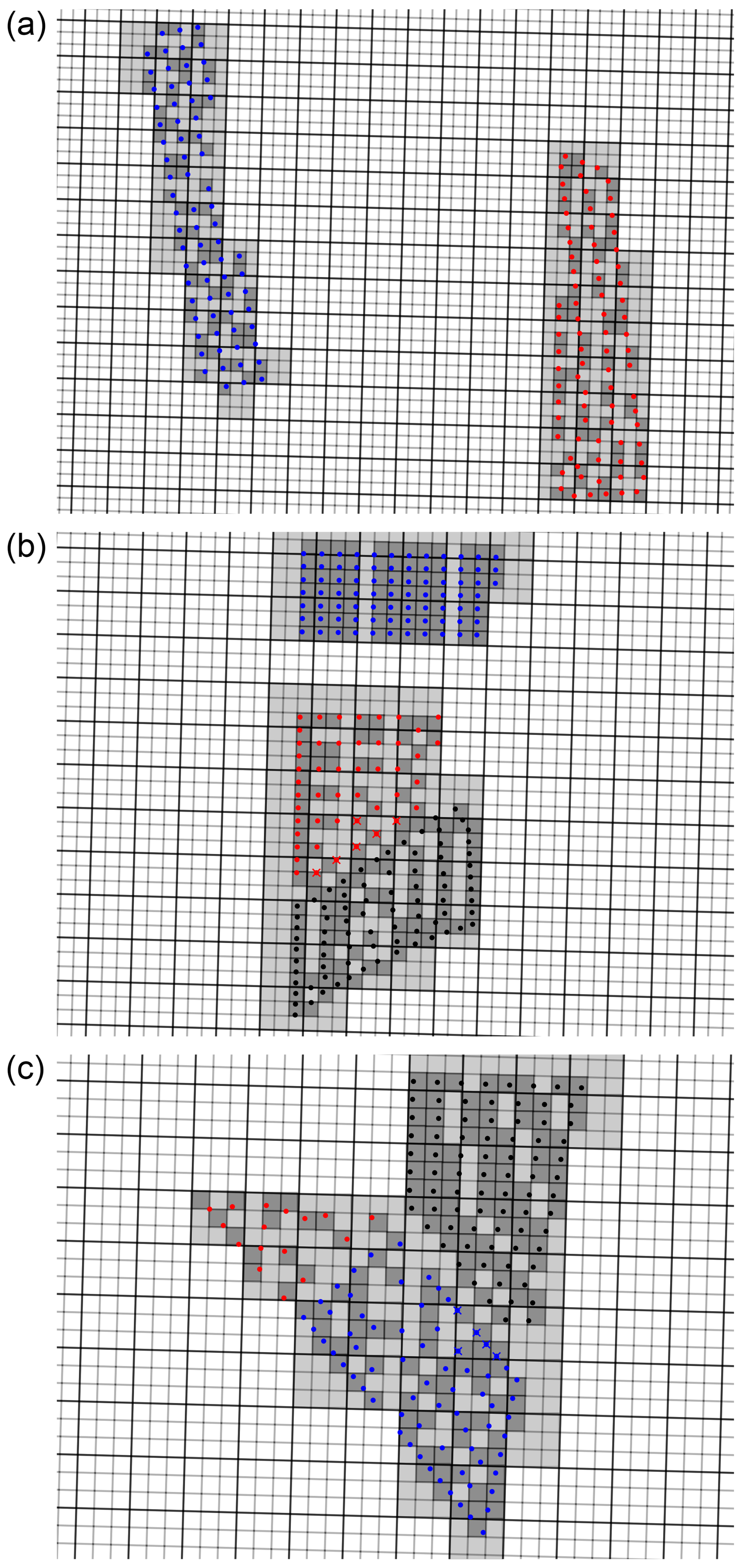
Figure B1 Layouts of wind farms on the WRF grid. (a) Sandbank (blue) and DanTysk (red). (b) Amrumbank West (blue) and Nordsee Ost (red), with Meerwind (black, not analyzed) to the south. (c) Hohe See (blue) and Albatros (red), with Global Tech One (black, not analyzed) to the northeast. Crosses indicate turbines that share a cell with turbines from another farm and are not considered in the analysis.