Enabling the use of unstructured meshes for the large-eddy simulation of stable atmospheric boundary layers

Modelling wind flows over complex terrain under varying atmospheric stability conditions is essential for improving our understanding of atmospheric boundary layer physics and its impact on wind energy systems. However, such simulations remain challenging due to the complexity of generating a mesh that matches complex geometries and the inherent difficulty of modelling the stable boundary layer, characterized by small-scale turbulent structures. To tackle this challenge, high-fidelity simulations with unstructured meshes, which offer great geometric flexibility, are used in this study. Nevertheless, unstructured grids are rarely used in atmospheric simulations. This study establishes a baseline framework for the use of unstructured meshes in atmospheric boundary layer simulations, with particular relevance to complex terrain. The proposed solver is validated against two well-established benchmarks under neutral and stable stratification. For the neutral case, the Andren benchmark, a $\mathrm{1.28}\times \mathrm{1.28}\times \mathrm{1.5}$ km³ periodic domain where the flow is driven by a large-scale pressure gradient, is considered. Results from structured and unstructured grids are in good agreement, with minor differences observed near the surface. Unstructured grids exhibit slightly higher friction velocities due to wall-proximal grid quality but remain within the expected variability of existing studies. The solver is then applied to the GABLS1 stable boundary layer case, a $\mathrm{400}\times \mathrm{400}\times \mathrm{400}$ m³ domain with surface cooling. Both grid types capture the evolution of the SBL, with unstructured grids yielding higher surface heat fluxes – up to 14 % – resulting in a thicker boundary layer and noticeable differences in mean profiles and fluxes. A mesh refinement study confirms that a horizontal resolution of Δx=6.25 m is sufficient for accurate SBL representation with both mesh types. Overall, the results demonstrate that unstructured meshes are a viable and robust tool for atmospheric boundary layer modelling, capable of matching the accuracy of structured grids while offering the flexibility required for complex terrain. The minor discrepancies observed remain within the variability expected from model formulation choices. This work thus provides a foundational reference for future high-fidelity atmospheric simulations using unstructured grids, particularly in terrain-resolving contexts.

1 Introduction

The global push toward renewable energy, driven by urgent environmental and energy concerns, has made maximizing wind farm efficiency a critical objective (IRENA, 2019). In response, wind turbine dimensions have increased dramatically, with rotor diameters now exceeding hundreds of metres. As a result, modern wind turbines are influenced not only by microscale atmospheric phenomena (scales below 1 km), but also by mesoscale processes, which span 5 to several hundred kilometres and govern local weather systems. These turbines now operate at the intersection of micro- and mesoscale dynamics (Veers et al., 2019). The extension across scales introduces new physical mechanisms that significantly affect atmospheric flow behaviour. At higher altitudes, flow is shaped by geostrophic balance, where the pressure gradient force – arising from synoptic-scale weather systems – is countered by the Coriolis force due to Earth's rotation. Closer to the ground, the structure of the atmospheric boundary layer (ABL) is strongly modulated by thermal stratification. Solar heating induces vertical temperature gradients that give rise to buoyancy-driven forces, classifying the atmosphere as stable, neutral, or unstable depending on the gradient's direction (Kaimal and Finnigan, 1994). Near the surface, terrain-induced effects become dominant, impacting both horizontal and vertical velocity gradients and generating complex features such as flow separation, recirculation zones, and spatially varying surface roughness. Understanding these multi-scale processes is crucial for improving the modelling and prediction of wind turbine performance, especially in heterogeneous environments. Despite extensive efforts, our knowledge of atmospheric flows over complex terrain remains incomplete (Elgendi et al., 2023).

Well-established factors influencing wind turbine behaviour are vertical wind shear and veer, which affect wake recovery (Abkar et al., 2018), wind turbine performance (Sanchez Gomez and Lundquist, 2020), and structural loads (Porté-Agel et al., 2020). While field campaigns and wind tunnel experiments offer valuable insights (Doubrawa et al., 2019; Moriarty et al., 2020), their practical application is constrained by cost and logistical complexity. Consequently, numerical simulations have become an increasingly prominent tool for studying atmospheric flows (Stoll et al., 2020). Large-eddy simulation (LES) is currently the state-of-the-art technique for resolving turbulent structures in the ABL. While LES of the convective boundary layer (CBL) is well established (Fernando and Weil, 2010), accurately simulating the stable boundary layer (SBL) remains a significant challenge (Mahrt, 2014). The difficulty stems from the relatively small characteristic length scales of turbulent structures in stable conditions. While the CBL can extend up to 1 km and is dominated by large convective eddies, the SBL typically remains confined below 200 m and is primarily driven by wind shear. The resulting turbulence is weaker, with finer-scale vortices requiring higher spatial resolution – and, by extension, increased computational resources – for accurate representation (Garratt, 1994).

In addition to thermal effects, simulating wind flows over complex terrain introduces further challenges, particularly in mesh generation. Several studies have used structured grids. As an example, Berg et al. (2018) performed LES over the Perdigao complex site and demonstrated that a realistic terrain representation is necessary, as a smoothed terrain could induce differences in wind speed of up to 19 %. Their structured mesh presents a vertical grid cell size expansion from the ground. However, building such a mesh remains difficult as both fine resolution and orthogonality are required. In Dar et al. (2019), a terrain-following coordinate transformation is used to represent the terrain. A similar method is employed in the Energy Research and Forecasting (ERF) code (Lattanzi et al., 2025), using a terrain-following coordinate system. However, this technique requires a terrain-smoothing step, which can induce uncertainty in simulation results (Klemp et al., 2003). In addition, when terrain slope increases, i.e. the grid becomes highly skewed, discretization errors can lead to numerical instabilities (Klemp, 2011). The immersed boundary method (IBM) is another technique used to accurately represent complex topography. Lundquist et al. (2012) have used WRF with an IBM approach to simulate flow over Oklahoma City. Arthur et al. (2020) have evaluated the IBM approach, highlighting the effectiveness of the method for steep terrain, particularly using fine grids. However, when using coarser resolution, near-surface velocity errors can occur. These methods, although functional and promising, have certain limitations.

Thus, in this work, we propose a different approach: the use of unstructured grids. Unstructured meshes offer greater flexibility in handling geometric complexity and local refinement (Bates et al., 2003; Bilskie et al., 2015) compared to structured ones. However, the development of high-fidelity solvers on unstructured grids – especially for LES – remains an area of active research, and their application to realistic atmospheric flows has been limited. To help bridge this gap, the present study investigates the use of unstructured grids for LES of the atmospheric boundary layer, with a focus on thermal stratification. Simulations are performed using both structured and unstructured meshes, enabling a direct comparison under controlled conditions. To the best of the authors' knowledge, this work represents the first LES of a stable boundary layer conducted on an unstructured mesh.

The paper is organized as follows. Section 2 outlines the numerical methodology. Section 3 presents neutral boundary layer simulations using both grid types with matching resolution. Section 4 extends the analysis to the stable boundary layer and includes a resolution sensitivity study. Final remarks and conclusions are provided in Sect. 5.

2 Methodology

2.1 Numerical framework

LESs are performed using the incompressible, constant-density flow solver of the YALES2 platform (Moureau et al., 2011), a high-performance, finite-volume code capable of handling both structured and unstructured meshes on massively parallel architectures. The spatial discretization relies on a fourth-order central differencing scheme, while time integration is performed using a fourth-order Runge–Kutta method (Kraushaar, 2011). Time integration is governed by a CFL condition: CFL<0.9.

The LES approach is based on the spatial filtering of the Navier–Stokes equations within the inertial range of turbulence. Using Einstein notation, and denoting the spatial filtering operator with a tilde ($\stackrel{\mathrm{̃}}{\cdot }$), the filtered incompressible Navier–Stokes equations are expressed as

$$\begin{array}{}\text{(1)}& \begin{array}{rl}{\displaystyle \frac{\partial {\stackrel{\mathrm{̃}}{\mathit{u}}}_i}{\partial x_i}}& =\mathrm{0}\text{and}{\displaystyle \frac{\partial {\stackrel{\mathrm{̃}}{\mathit{u}}}_j}{\partial t}}+{\displaystyle \frac{\partial {\stackrel{\mathrm{̃}}{\mathit{u}}}_i{\stackrel{\mathrm{̃}}{\mathit{u}}}_j}{\partial x_i}}=\mathit{\nu }{\displaystyle \frac{{\partial }^{\mathrm{2}}\stackrel{\mathrm{̃}}{\mathit{u}}j}{\partial x_i\partial x_i}}+{\displaystyle \frac{\mathrm{1}}{{\mathit{\rho }}_{\mathrm{0}}}}{\displaystyle \frac{\partial \mathit{\tau }i{j}^R}{\partial x_i}}\\ & -{\displaystyle \frac{\mathrm{1}}{{\mathit{\rho }}_{\mathrm{0}}}}{\displaystyle \frac{\partial \stackrel{\mathrm{̃}}{P}}{\partial x_j}}+{\displaystyle \frac{\stackrel{\mathrm{̃}}{\mathit{\theta }}-{\mathit{\theta }}_{\mathrm{0}}}{{\mathit{\theta }}_{\mathrm{0}}}}{g}_j-\mathrm{2}\mathrm{\Omega }({\mathit{G}}_j-{\stackrel{\mathrm{̃}}{\mathit{u}}}_j),\end{array}\end{array}$$

where u is the velocity vector, ν the kinematic viscosity, ${\mathit{\tau }}_{ij}^R$ the subgrid-scale (SGS) stress tensor, and P the pressure. The last two terms on the right-hand side represent buoyancy and Coriolis effects under the Boussinesq approximation (Gray and Giorgini, 1976), where θ is the potential temperature, g the gravitational acceleration, Ω Earth's angular velocity, and G the geostrophic wind vector. ρ₀ and θ₀ refer to the reference air density and potential temperature, respectively. The potential temperature evolution follows the classical transport diffusion equation

$$\begin{array}{}\text{(2)}& {\displaystyle \frac{\partial \stackrel{\mathrm{̃}}{\mathit{\theta }}}{\partial t}}+{\displaystyle \frac{\partial \stackrel{\mathrm{̃}}{\mathit{\theta }}}{\partial x_i}}={\mathit{\alpha }}_{\mathrm{0}}{\displaystyle \frac{{\partial }^{\mathrm{2}}\stackrel{\mathrm{̃}}{\mathit{\theta }}}{\partial x_i\partial x_i}}\text{,}\end{array}$$

where α₀ is the thermal diffusivity at the reference state.

Subgrid-scale turbulence is modelled using the dynamic Smagorinsky model (Germano et al., 1991; Lilly, 1992), which adjusts the Smagorinsky constant based on local flow characteristics. Although more advanced models exist for capturing anisotropic turbulence (Gadde et al., 2021), the dynamic Smagorinsky model remains widely used due to its simplicity and robustness (Pope, 2001). Notably, it has demonstrated improved performance in reproducing stable boundary layer dynamics, including greater boundary layer depth compared to the original Smagorinsky formulation (Beare et al., 2006).

2.2 Wall model

Due to mesh resolution limitations near the surface, the near-wall region is not fully resolved. Instead, a wall model based on the Monin–Obukhov similarity theory (MOST) (Monin and Obukhov, 1954; Landau and Lifshitz, 1959) is employed to compute surface momentum and heat fluxes. MOST provides a unified framework capable of capturing all three stability regimes – neutral, stable, and unstable – via correction functions in the logarithmic velocity and temperature profiles (Kaimal and Finnigan, 1994).

The velocity and temperature profiles are given by

$$\begin{array}{}\text{(3)}& {\displaystyle \frac{u\left(z\right)}{u_{*}}}={\displaystyle \frac{\mathrm{1}}{\mathit{\kappa }}}\left[\ln \left({\displaystyle \frac{z}{z_{\mathrm{0}}}}\right)-{\mathit{\psi }}_m\left({\displaystyle \frac{z-z_{\mathrm{0}}}{L}}\right)\right],\text{(4)}& {\displaystyle \frac{\mathit{\theta }\left(z\right)-{\mathit{\theta }}_{\mathrm{w}}}{{\mathit{\theta }}_{*}}}={\displaystyle \frac{\mathrm{1}}{\mathit{\kappa }}}\left[\ln \left({\displaystyle \frac{z}{z_{\mathrm{0}}}}\right)-{\mathit{\psi }}_h\left({\displaystyle \frac{z-z_{\mathrm{0}}}{L}}\right)\right],\end{array}$$

where $u_{*}=\sqrt{{\mathit{\tau }}_{\mathrm{w}}/\mathit{\rho }}$ is the friction velocity, with τ_w being the local shear stress at the wall. ${\mathit{\theta }}_{*}=-q_{\mathrm{w}}/u_{*}$ is the friction temperature, with q_w being the kinematic surface heat flux and θ_w the wall temperature. κ is the von Kármán constant and z₀ the roughness length. The absolute value of the Obukhov length L characterizes the height at which buoyancy effects begin to dominate over shear and is computed as $L=-\frac{u_{*}^{\mathrm{3}}{\mathit{\theta }}_{\mathrm{0}}}{\mathit{\kappa }g{q}_{\mathrm{w}}}$, where θ₀=263.5 K is the reference potential temperature.

The correction functions ψ_m and ψ_h are set to zero for neutral cases, leading to a classical logarithmic velocity profile. For non-neutral configurations, they can be expressed as

$$\begin{array}{}\text{(5)}& {\mathit{\psi }}_{m/h}\left(\mathit{\xi }\right)=\underset{z_{\mathrm{0}}/L}{\overset{\mathit{\xi }}{\int }}{\displaystyle \frac{\mathrm{1}-{\mathit{\varphi }}_{m/h}\left(\mathit{\xi }\right)}{\mathit{\xi }}}\mathrm{d}z,\end{array}$$

where $\mathit{\xi }=z/L$, and ϕ_m and ϕ_h are termed stability functions. The latter are empirically determined depending on the stability condition. For stable cases they are expressed as

$$\begin{array}{}\text{(6)}& \begin{array}{rl}{\displaystyle }{\mathit{\varphi }}_m& {\displaystyle }=\mathrm{1}+{\mathit{\beta }}_m\mathit{\xi },\\ {\displaystyle }{\mathit{\varphi }}_h& {\displaystyle }=\mathrm{1}+{\mathit{\beta }}_h\mathit{\xi }.\end{array}\end{array}$$

Various parameterizations have been introduced over the years (Businger, 1971; Högström, 1988). In this work, we use the one prescribed in the GABLS1 setup: β_m=4.8 and β_h=7.8.

Following the approach of Basu et al. (2008), the wall temperature is prescribed as a boundary condition rather than the surface heat flux. This introduces a coupled system with two unknowns: the friction velocity u_* and the heat flux q_w. They are solved using a double Newton–Raphson algorithm (Ypma, 1995), selected for its quadratic convergence properties.

As the wall model is derived from filtered equations, inputs such as velocity and temperature must be appropriately averaged. For structured meshes, horizontal-plane averaging at the first grid point above the surface is straightforward. In unstructured meshes, where such planes do not exist, spatial filtering is achieved using a gather–scatter operator applied between control volumes and nodal points (Larsson et al., 2016).

2.3 Grid generation

In the following studies, two grid types are used: structured (S) and unstructured (U). A constant cell size in all three directions is used. For structured meshes, this translates to a 3D Cartesian mesh with a constant cell size, using hexahedra elements. For unstructured meshes, a 3D grid using tetrahedral elements is created using the GMSH mesh generator tool (Geuzaine and Remacle, 2009). A visualization of both meshes, based on the meshes used in Sect. 4, is shown in Fig. 1. Similar meshes are used in Sect. 3; only the domain size and the mesh size differ.

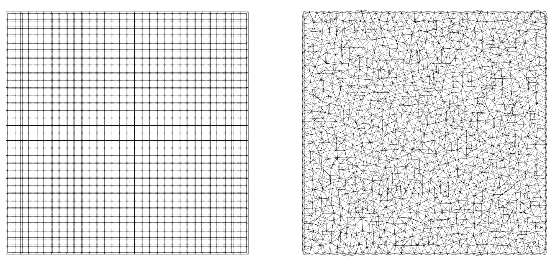
Figure 1 x−z crinkle slice at y=200 m for the Δx=12.5 m cell size mesh used in Sect. 4. Left: structured grid, right: unstructured grid.

YALES2 defines control volumes at the nodes. In order to make meaningful comparisons, in the next studies the number of nodes – and therefore the degrees of freedom – between structured and unstructured meshes is similar. This translates into a significantly different number of elements depending on the element type.

Details about unstructured-mesh quality can be found in Sect. 4.2.1. It explains some of the differences measured between the simulations obtained on the two types of meshes.

3 Neutral boundary layer

To establish the validity of the use of unstructured meshes for atmospheric simulations, an initial benchmark test is conducted under truly neutral stratification. For this purpose, the well-known case developed by Andren et al. (1994) is reproduced and serves as a reference.

3.1 Case description

The simulation domain is a rectangular box of $\mathrm{1280}\times \mathrm{1280}\times \mathrm{1500}$ m³, as illustrated by Fig. 2. Periodic boundary conditions are applied in the horizontal directions to emulate an infinite atmospheric boundary layer. A slip wall is prescribed at the domain top, while a rough bottom boundary with roughness length z₀=0.1 m is modelled using Monin–Obukhov. The flow is driven by geostrophic forcing, with the geostrophic wind vector set to $(G_x,G_y)=(\mathrm{10},\mathrm{0})$ m s⁻¹ and the Coriolis parameter specified as $f={\mathrm{10}}^{-\mathrm{4}}$ s⁻¹. Simulations were initialized with a reference density of ρ₀=1 kg m⁻³. The initial velocity field is defined following the original configuration from Andren et al. (1994):

$$\begin{array}{}\text{(7)}& \begin{array}{l}u\left(z\right)=G_x\left(\mathrm{1}-\exp \left(-\frac{z}{L_z}\right)\cos \left(\frac{z}{L_z}\right)\right),\\ v\left(z\right)=G_x\exp \left(-\frac{z}{L_z}\right)\cos \left(\frac{z}{L_z}\right).\end{array}\end{array}$$

The simulation results are compared to those of four previous studies (Andren et al., 1994; Chow et al., 2005; Senocak et al., 2007; Feng et al., 2021).

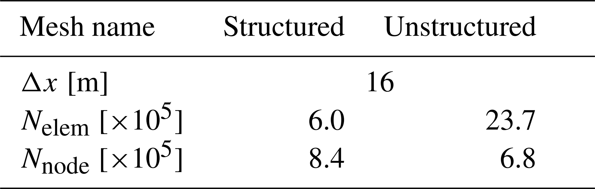
The simulation is run for a 30 dimensionless time period tf as in Chow et al. (2005), equivalent to 84 physical hours. Statistical quantities are averaged over the final six dimensionless time periods, equivalent to 28 h. It approximately corresponds to the inertial oscillation period $\mathrm{2}\mathit{\pi }/f$. Senocak et al. (2007) showed that it was enough for the statistics to remain fairly stationary during the averaging period. The grid resolution is set to Δ=16 m, consistent with Feng et al. (2021) and comparable to Senocak et al. (2007). Chow et al. (2005) employed a vertically refined mesh, while Andren et al. (1994) used slightly coarser grids. Table 1 summarizes the grid sizes, the number of elements, and the number of nodes. As stated in Sect. 2.3, to ensure a fair comparison between mesh types, the number of nodes is comparable.

Table 1 Case setup with Δx being the mesh cell size, N_elem the number of mesh elements, and N_node the number of mesh nodes.

3.2 Results

Figure 2b shows the time-averaged and horizontally averaged streamwise velocity profile, computed over the final 28 h of the simulation to ensure statistical stationarity. The velocity profile exhibits the expected logarithmic shape characteristic of a neutrally stratified boundary layer. This profile reflects the balance between surface friction and the geostrophic pressure gradient. Results obtained using both structured and unstructured meshes demonstrate excellent agreement with reference studies, indicating that the large-scale flow dynamics are well captured regardless of mesh type. Differences between mesh types are negligible in this case.

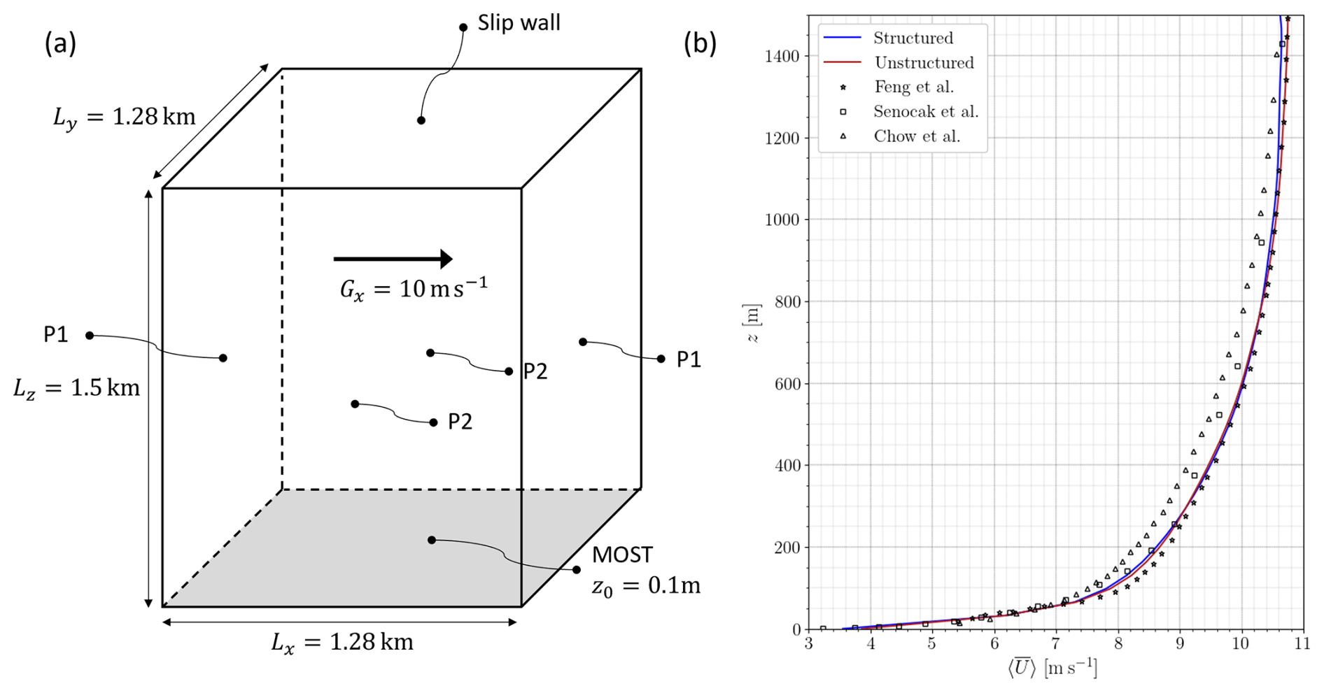
Figure 2 (a) Andren setup configuration scheme. P1 and P2 represent periodic boundaries in pairs. (b) Average velocity profile of the Andren case gathered in 28 h.

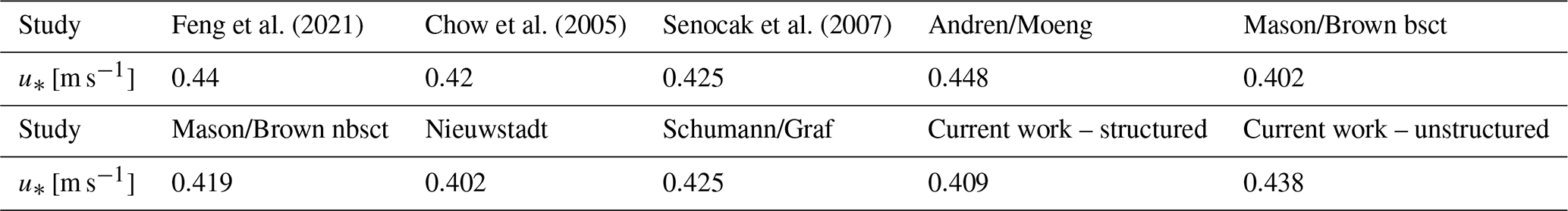
Quantitative comparison of the surface friction velocity, u_*, is provided in Table 2. For the structured-mesh simulation, $u_{*}=\mathrm{0.409}$ m s⁻¹, while the unstructured mesh yields a slightly higher value of $u_{*}=\mathrm{0.438}$ m s⁻¹. These results fall within the range reported in the four prior studies. The slightly elevated value observed in the unstructured-grid simulation can be attributed to the irregularity of the unstructured mesh near the wall. This irregularity complicates the accurate evaluation of wall-normal gradients and, combined with uneven variations in the first fluid node height, results in cell-to-cell fluctuations in the momentum flux. This effect is particularly pronounced in double-periodic domains, where maintaining mesh regularity is more challenging. Lower mesh quality in the near-wall region can thus amplify momentum transfer, thereby increasing surface stress and the corresponding friction velocity.

Feng et al. (2021)Chow et al. (2005)Senocak et al. (2007)

Table 2 Frictional velocity for the four different studies. Andren/Moeng, Mason/Brown, Nieuwstadt, and Schumann/Graf refer to the four distinct LES codes used in Andren et al. (1994).

To further assess flow characteristics, Fig. 3 shows time-averaged and horizontally averaged vertical profiles of the streamwise velocity variance $\stackrel{\mathrm{‾}}{\langle {u^{\prime }}^{\mathrm{2}}\rangle }$ and the Reynolds shear stress $\langle \stackrel{\mathrm{‾}}{u^{\prime }{w}^{\prime }}\rangle$. Results from both structured- and unstructured-mesh simulations are compared to the spread reported in the reference studies. In both cases, the profiles fall within the variability range found in the literature. However, the unstructured-mesh simulation exhibits slightly higher velocity variance near the wall. This is consistent with the previously observed higher surface friction velocity, as enhanced near-surface shear naturally leads to stronger velocity fluctuations. While these differences are measurable, they remain smaller than the broader inter-study variability, which arises from differing numerical schemes, subgrid-scale models, and wall treatment methods.

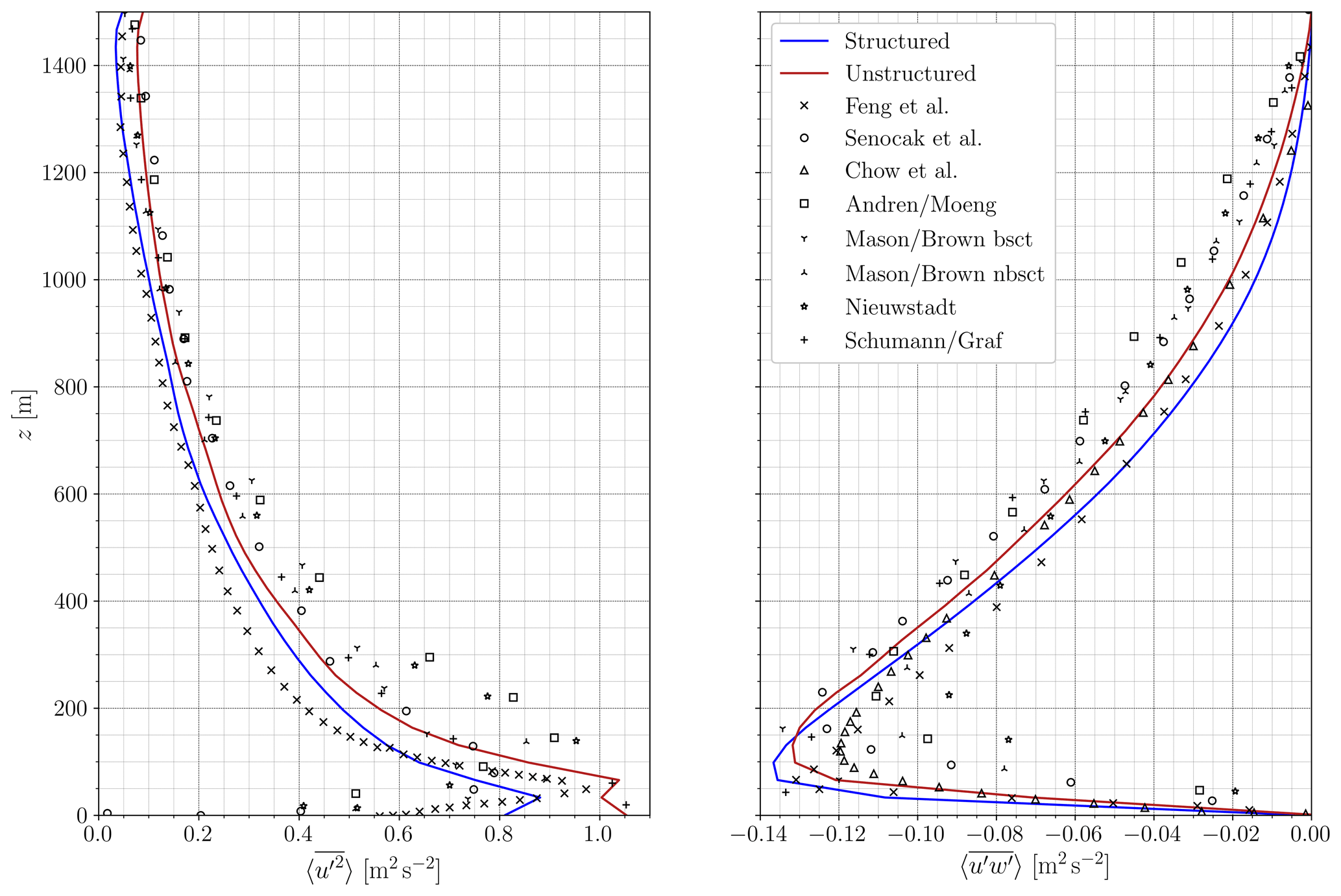
Figure 3 Time-averaged and horizontally averaged streamwise velocity variance and momentum flux profile of the Andren case gathered in 28 h.

This simple neutral configuration serves as a first validation step for the proposed methodology. The results demonstrate that the methodology using unstructured meshes is capable of accurately reproducing the dynamics of a neutral atmospheric boundary layer. All key flow quantities fall within the range of previous studies, confirming the robustness of the approach. No mesh sensitivity study has been conducted for this neutral case. As turbulent structures are relatively large and easier to resolve, a fine mesh is unnecessary. However, the results still highlight the influence of the mesh, particularly near the wall. The next step focuses on the stable boundary layer, where thermal stratification introduces additional physical challenges and where mesh resolution plays a more critical role in capturing the finer turbulent structures.

4 Stable boundary layer

To improve our understanding of the stable atmospheric boundary layer and its representation in LES, the Global Energy and Water Cycle Experiment (GEWEX) launched the GEWEX Atmospheric Boundary Layer Study (GABLS) (Holtslag et al., 2012). The GABLS initiative has focused on land-based SBLs and the accurate simulation of their diurnal cycle. Over time, three benchmark intercomparison cases have been defined, progressively increasing in realism (Sanz Rodrigo et al., 2017). This study adopts the first intercomparison case, known as GABLS1, which targets an idealized Arctic SBL scenario (Kosović and Curry, 2000).

4.1 Case description

The original GABLS1 intercomparison involved 11 LES codes and demonstrated that accurate resolution of the SBL strongly depends on mesh resolution (Beare et al., 2006). Follow-up studies have employed the GABLS1 setup to investigate the influence of grid refinement (Sullivan et al., 2016; Min and Tombouldies, 2022), surface cooling rates (Sullivan et al., 2016; Kumar et al., 2010; Huang and Bou-Zeid, 2013), and subgrid-scale modelling strategies (Matheou and Chung, 2014; Ghaisas et al., 2017; Gadde et al., 2021). Additional research has used GABLS1 as a validation benchmark for Reynolds-averaged Navier–Stokes (RANS) models and pseudo-spectral LES methods (Sanz Rodrigo et al., 2017; Lazeroms, 2015). While previous studies have successfully reproduced key SBL characteristics, they have all employed structured meshes. To the best of the authors' knowledge, no study has yet explored the use of unstructured grids for this configuration, likely due to the relatively simple geometry of the domain. In this work, we assess the capability of unstructured meshes to replicate the GABLS1 benchmark results, and we compare them directly against structured-mesh simulations at matched spatial resolutions.

The computational domain measures $\mathrm{400}\times \mathrm{400}\times \mathrm{400}$ m³, with periodic boundary conditions in the streamwise (x) and spanwise (y) directions. The bottom boundary is a rough wall, with a surface roughness length of z₀=0.1 m and a fixed surface temperature T_w=265 K. A constant cooling rate of 0.25 K h⁻¹ is imposed. The top boundary is treated as a stress-free slip wall. A geostrophic wind of G_x=8 m s⁻¹ is applied in the x direction. A Coriolis parameter of $f=\mathrm{1.39}\times {\mathrm{10}}^{-\mathrm{4}}$ s⁻¹ is prescribed, corresponding to a latitude of 73° N. Other physical parameters include gravity g=9.81 m s⁻², reference potential temperature θ₀=263.5 K, air density ρ₀=1.3223 kg m⁻³, and the von Kármán constant κ=0.4. Figure 4 illustrates the domain configuration and initial profiles.

The initial velocity field is set to the geostrophic wind throughout the domain. The temperature profile is initialized at 265 K in the lower 100 m and increases linearly by 0.01 K m⁻¹ above that height, reaching 268 K at the top. To initiate turbulence, random perturbations of amplitude 0.1 K are added to the temperature field within the lowest 50 m, as described in Beare et al. (2006).

To damp gravity wave reflection near the upper boundary, a sponge layer is implemented above 300 m. This layer relaxes velocity and temperature fields toward their initial target profiles using the following formulation:

$$\begin{array}{}\text{(8)}& {\mathrm{SL}}_{\mathit{\varphi }}=\mathit{\gamma }{\sin }^{\mathrm{2}}\left({\displaystyle \frac{z-Z_{\mathrm{SL}}}{L_z-Z_{\mathrm{SL}}}}{\displaystyle \frac{\mathit{\pi }}{\mathrm{2}}}\right)({\mathit{\varphi }}_{\mathrm{target}}-\mathit{\varphi }),\end{array}$$

where ϕ represents either the velocity or the temperature, ϕ_target denotes the target (geostrophic or stratified) profile, and $\mathit{\gamma }=\mathrm{1}/\mathrm{5}$ is a time relaxation parameter. The vertical range of the sponge layer extends from z_SL=300 m to the domain top at z_top=400 m.

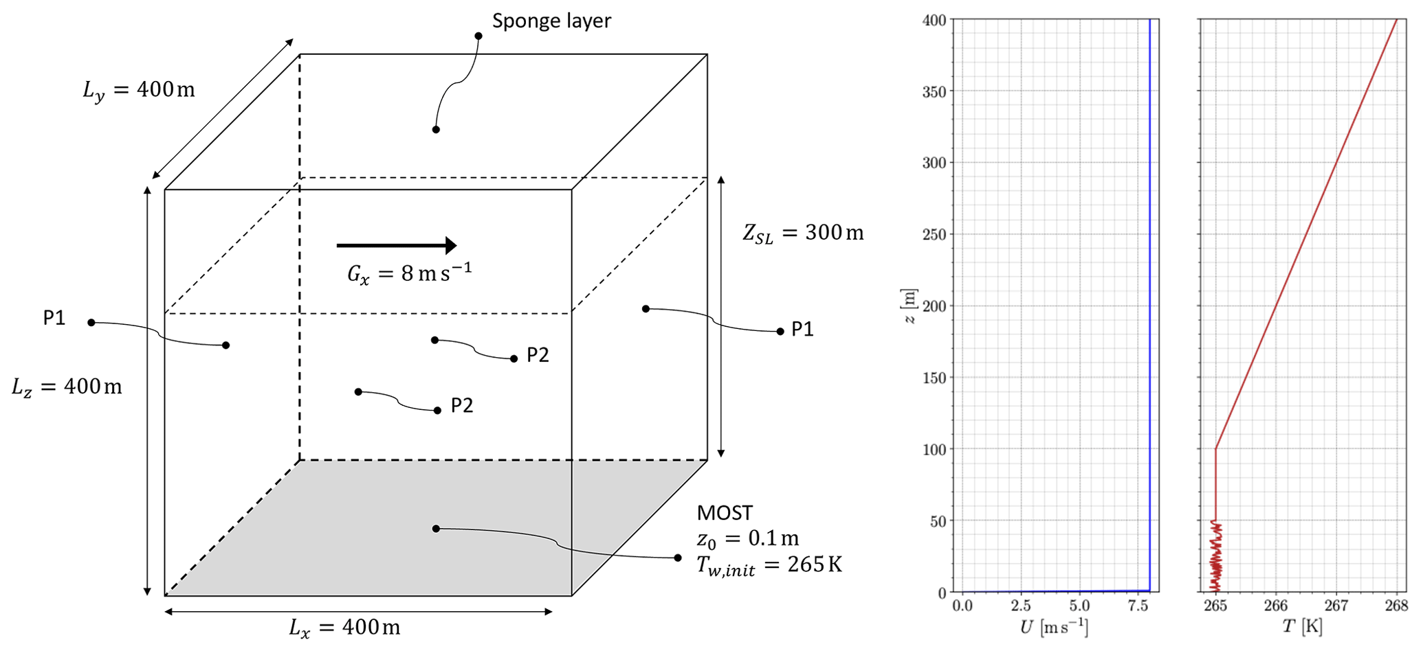
Figure 4 (a) GABLS1 setup configuration scheme. P1 and P2 represent periodic boundaries in pairs. (b) Initial velocity and temperature vertical profiles.

For stable boundary layer simulations, the CFL is modified in accordance with shallow-water models (Walters et al., 2009). Due to the explicit integration of the Coriolis force, the time step is here chosen following the approach of Audusse et al. (2018) such that $\mathrm{\Delta }t=\frac{\mathrm{CFL}\times \mathrm{\Delta }x}{\left|U\right|+\sqrt{gH}}$, with H being the vertical depth of the fluid, i.e. the stable boundary layer height. The CFL condition remains CFL<0.9. Convective velocity and boundary layer height are chosen in accordance with the a priori values of the upcoming simulations: $\left|U\right|=\mathrm{9}$ m s⁻¹ and H=200 m, respectively. All time steps used in this study are summarized in Table 3.

Simulations are run for a total of 8 h of physical time, corresponding to a full diurnal cycle. Statistics are gathered during the final hour of simulation (between hour 7 and 8), once quasi-stationary conditions are achieved. Results are compared with the original GABLS1 intercomparison (Beare et al., 2006), as well as a wide range of follow-up studies (Kumar et al., 2010; Huang and Bou-Zeid, 2013; Matheou and Chung, 2014; Sullivan et al., 2016; Abkar and Moin, 2017; Ghaisas et al., 2017; Gadde et al., 2021; Dai et al., 2021).

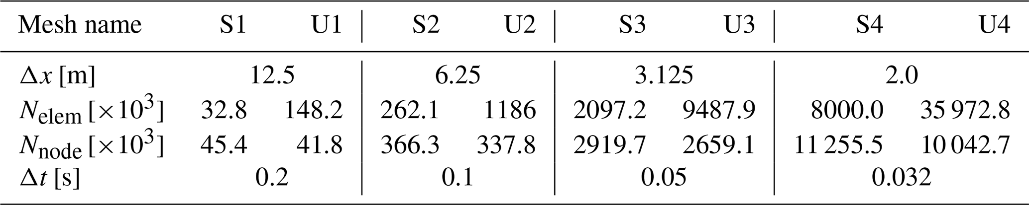
Structured and unstructured meshes at four different spatial resolutions are employed. Table 3 summarizes the grid sizes, number of elements, number of nodes, and the corresponding time step. As stated in Sect. 2.3, to ensure a fair comparison between mesh types, the number of nodes is comparable.

Table 3 Case setup with Δx being the mesh cell size, N_elem the number of mesh elements, N_node the number of mesh nodes, and Δt the time step.

4.2 Results

4.2.1 Unstructured- and structured-grid comparison

Following the GABLS1 recommendations (Beare et al., 2006), a cell size of Δx=3.125 m is used for both mesh types. The structured and unstructured grids are referred to as S3 and U3, respectively (see Table 3).

Figure 5 shows the temporal evolution of key surface layer quantities: friction velocity (u_*), wall heat flux (Q_w), and Monin–Obukhov length (L). All time series lie within the range of the GABLS1 intercomparison dataset (Beare et al., 2006), indicating overall agreement with previous LES studies. The friction velocity is similar for both grids throughout the simulation, with S3 producing slightly lower values than U3. This observation is consistent with results in the neutral boundary layer and indicates that the error in gradient estimation associated with grid type remains modest. Notably, the U3 simulation closely matches results from the PALM model (Dai et al., 2021), a widely adopted LES code in atmospheric modelling.

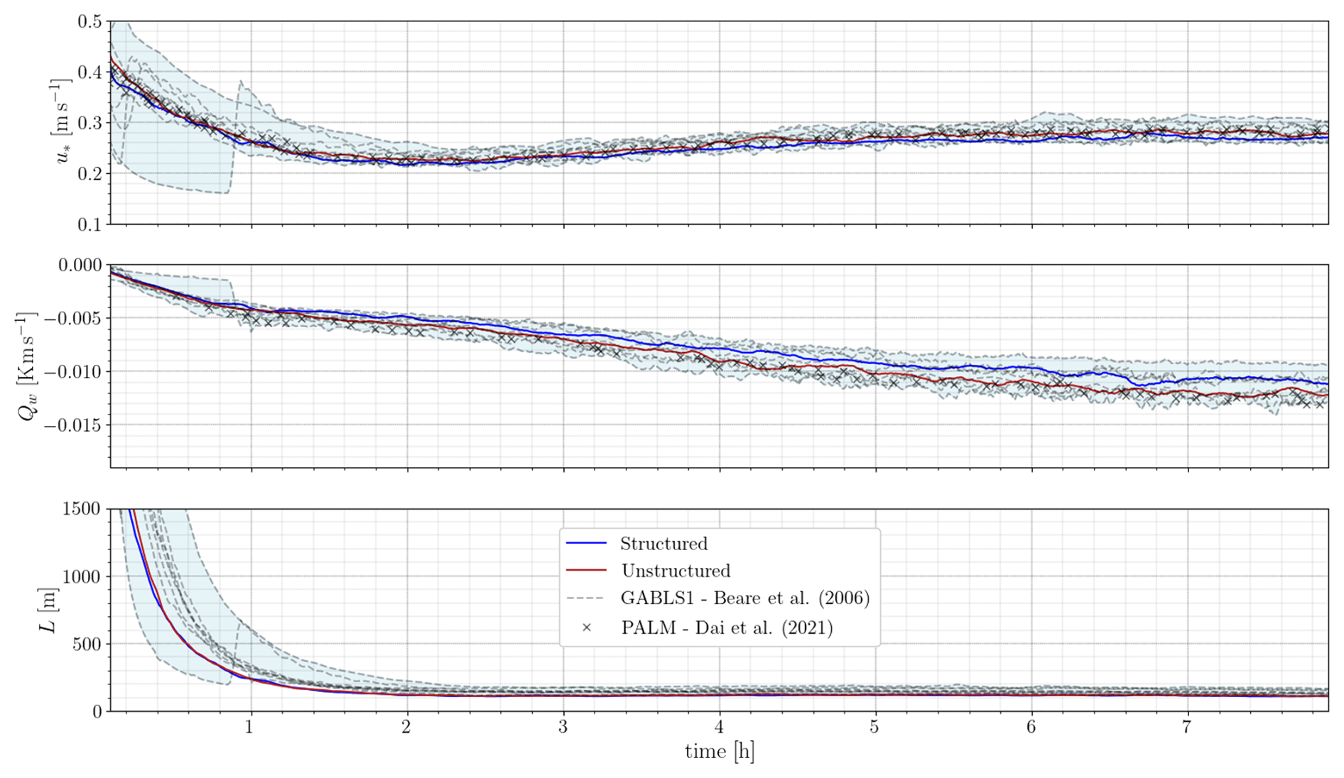
Figure 5 Frictional velocity, wall heat flux, and Monin–Obukhov length with S3 and U3 grids compared to original GABLS1 result dispersion (Beare et al., 2006) and PALM results (Dai et al., 2021).

The Monin–Obukhov length exhibits similar trends for both meshes. After an initial rapid decrease due to surface cooling, L stabilizes at O(100) m. Wall heat fluxes show a general decay over time in both cases. However, a gap develops after the first hour, reaching a maximum difference of approximately 14 % between the 7th and 8th simulation hour. This divergence likely reflects differences in near-wall numerical behaviour caused by mesh structure.

In addition to this mesh-induced difference, another source of error could be the initial temperature perturbations. Indeed, after initialization, the flow destabilizes and transitions from a laminar to a turbulent stable boundary layer. This process is sensitive to the initial temperature perturbations, which differ slightly across simulations due to the imposed random fields. This sensitivity is further discussed in Appendix A. It could contributes to divergence among simulations. Some of the larger excursions observed in the original GABLS1 ensemble (see Fig. 5) may result from similar effects.

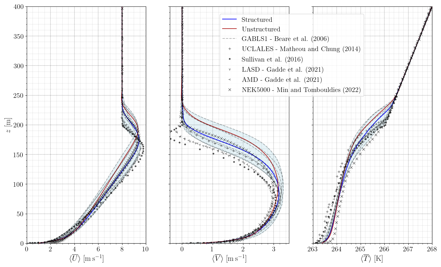
Figure 6 Time-averaged and horizontally averaged streamwise velocity and tangential velocity and temperature profiles for meshes S3 and U3 with cell size Δx=3.125 m. The blue-shaded area stands for the original GABLS1 study result dispersion (Beare et al., 2006) and symbols for more recent studies (Matheou and Chung, 2014; Sullivan et al., 2016; Gadde et al., 2021; Min and Tombouldies, 2022).

The time-averaged and horizontally averaged profiles of streamwise velocity U, tangential velocity V, and potential temperature θ are shown in Fig. 6. Averaging is performed between the 7th and 8th simulation hour, following the GABLS1 protocol. The velocity profiles exhibit a well-formed stable boundary layer, with a low-level jet located between 160 and 200 m. The tangential velocity grows with decreasing height due to Coriolis acceleration and vanishes at the surface under the action of surface drag. The temperature increases with height, with a distinct inversion layer forming between 150 and 200 m.

Differences between S3 and U3 results are visible but fall within the GABLS1 spread. The U3 simulation shows a 20 m upward shift in the velocity peak and corresponding temperature inflection point, indicating a slightly deeper or displaced SBL structure. Similar variations are found in more recent LES studies, which also broaden the envelope of acceptable solutions. For instance, the simulation by Sullivan et al. (2016) shows a negative tangential velocity near the top of the SBL that remains unexplained. Such discrepancies underscore the challenge of defining unique reference data for the SBL but also validate the fidelity of both S3 and U3 configurations.

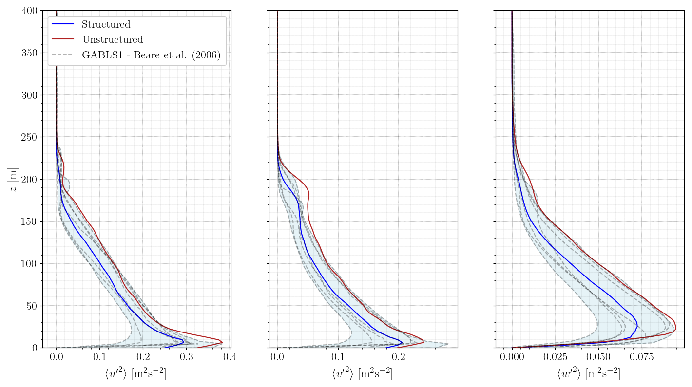
Figure 7 Time-averaged and horizontally averaged streamwise, tangential, and vertical velocity variance profiles with S3 and U3 of cell size Δx=3.125 m. Blue shading stands for the original GABLS1 study result dispersion (Beare et al., 2006).

Figure 7 displays the time-averaged and horizontally averaged velocity variances for all three components. Variances are higher in the lowest part of the boundary layer – the region with turbulence production – except near the surface where they are suppressed by the wall model. In the geostrophic region, turbulent motions decrease to zero, defining a zone comparable to the free atmosphere. Across all velocity components, the U3 mesh consistently exhibits higher variance levels than S3.

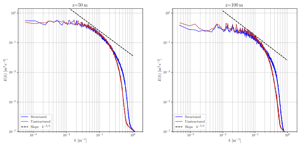
Figure 8 Energy spectra for structured (S3) and unstructured (U3) meshes at two different heights: z=50 m (left) and z=100 m (right). The Kolmogorov $\mathrm{-}\mathrm{5}/\mathrm{3}$ reference slope is plotted to identify the inertial subrange.

To understand these differences, the resolved turbulent kinetic energy spectrum is plotted in Fig. 8 for both structured and unstructured grids, using measurements at multiple horizontal locations extracted at two vertical positions: z=50 and z=100 m. At both heights, the spectral content matches between mesh types. The largest flow structures, corresponding to low frequencies, are well represented. Both spectra follow the theoretical ${\mathit{\kappa }}^{\mathrm{-}\mathrm{5}/\mathrm{3}}$ trend over a limited range of wave numbers, confirming that the inertial cascade is correctly reproduced. Minor differences can be noted at higher frequencies, where the unstructured-grid simulation exhibits spectra that decrease faster than those of the structured-grid simulation, resulting in a slightly smaller magnitude at the highest wave numbers. This discrepancy is probably due to slightly greater numerical diffusion of the unstructured grid. Velocity variance differences are thus not the result of inaccuracies in the energy cascade resolution.

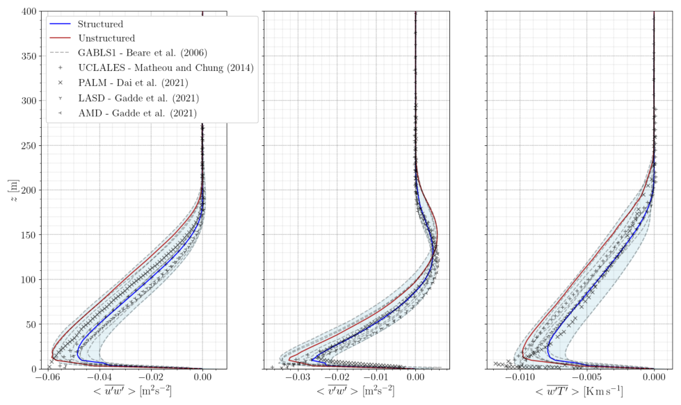
Figure 9 Time-averaged and horizontally averaged momentum and heat flux profiles for meshes S3 and U3 with cell size Δx=3.125 m. Blue shading stands for the original GABLS1 study result dispersion (Beare et al., 2006) and symbols for more recent studies (Matheou and Chung, 2014; Dai et al., 2021; Gadde et al., 2021).

The time-averaged and horizontally averaged momentum fluxes, $\langle \stackrel{\mathrm{‾}}{u^{\prime }{w}^{\prime }}\rangle$ and $\langle \stackrel{\mathrm{‾}}{v^{\prime }{w}^{\prime }}\rangle$, and heat flux, $\langle \stackrel{\mathrm{‾}}{w^{\prime }{T}^{\prime }}\rangle$, are plotted in Fig. 9. All fluxes follow expected vertical trends and are consistent with past studies. As with the velocity variances, the U3 simulation shows a vertical offset associated with greater turbulent transport.

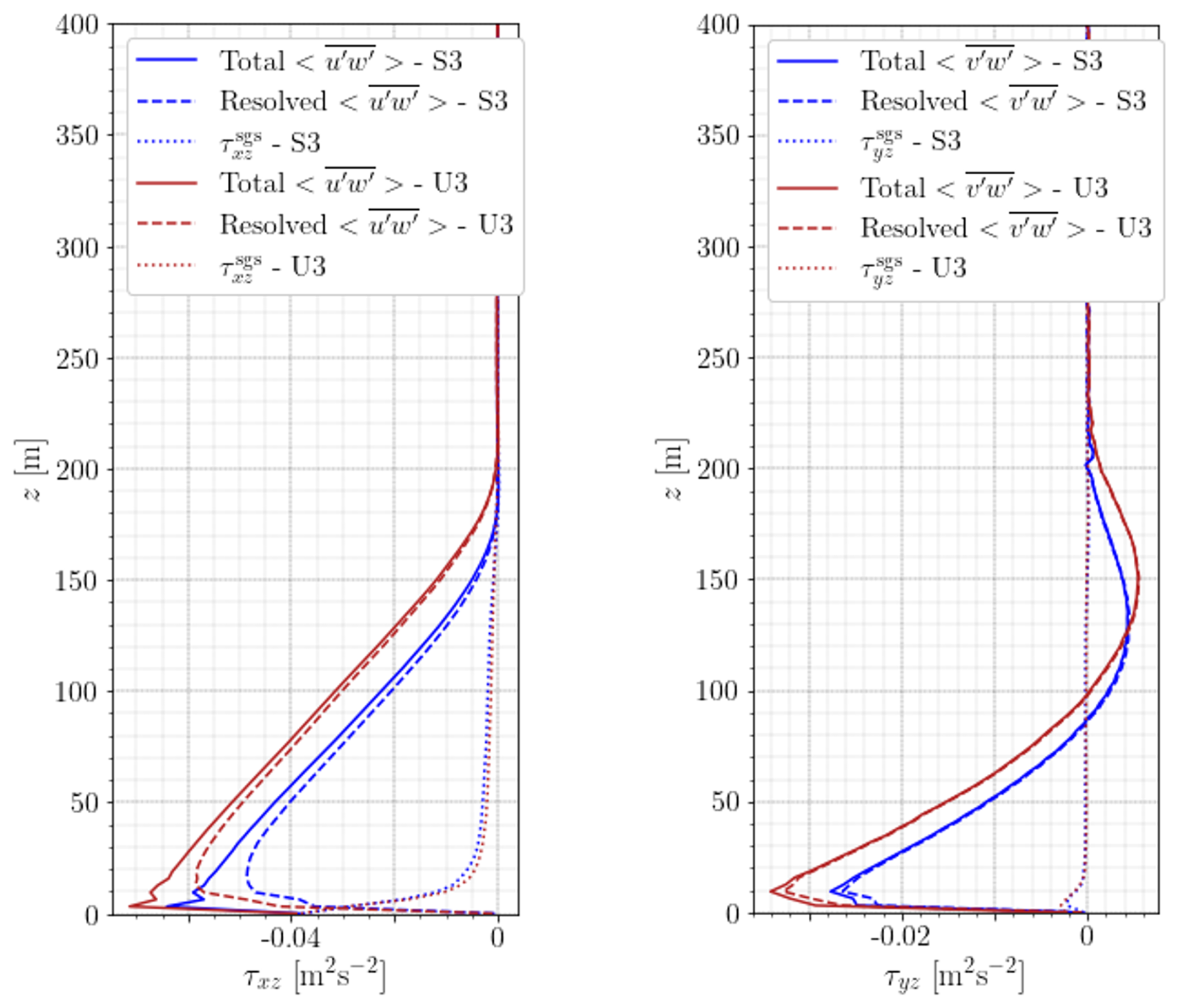
Figure 10 Comparison of total, resolved, and SGS fluxes of $\langle \stackrel{\mathrm{‾}}{u^{\prime }{w}^{\prime }}\rangle$ (left) and $\langle \stackrel{\mathrm{‾}}{v^{\prime }{w}^{\prime }}\rangle$ (right) for both S3 and U3 meshes.

While Fig. 9 only represents the resolved turbulence stresses, Fig. 10 displays the total, resolved, and modelled momentum fluxes to identify the differences in SGS model impact on the solution between structured- and unstructured-mesh simulations. In both momentum fluxes, the resolved and total turbulence stresses are nearly identical. The modelled turbulence stresses are negligible everywhere, except near the wall where their contribution locally reaches a maximum value of 10 % of the total stress. This expected behaviour shows that the grid size is refined enough to properly capture the boundary layer across the domain. However, near the wall, higher fluctuations could require an even more refined mesh. This result is in agreement with Beare et al. (2006), stating that a Δx=3.125 m resolution was necessary for a high-fidelity simulation of this case. In addition, this result confirms that the observed discrepancies in the resolved turbulence fluxes are also visible for total turbulence fluxes and not due to the SGS contribution.

Overall, these diagnostics reveal that the differences between mesh types are not of physical origin, i.e. related to the resolution of turbulence, but rather due to numerical effect. The observed discrepancies may arise from three primary sources:

• Grid quality. Although S3 and U3 share the same nominal resolution, the unstructured mesh introduces local geometric irregularities. Figure 11 shows the skewness and aspect ratio distribution and illustrates the spatial cell size distribution using a 2D plane for the U3 mesh. Most U3 cells have acceptable quality with a global mean skewness of 0.3, but up to 0.5 % of cells exceed a skewness of 0.8 and can even locally reach values of 0.96. The aspect ratio follows a similar trend: most elements have an aspect ratio close to unity, but 0.5 % of cells exceed an aspect ratio of 3.

• Numerical scheme accuracy. While perfectly fourth order on structured meshes, the accuracy of numerical schemes slightly deteriorates on unstructured grids due to mesh geometric non-uniformity and may locally reach third order. As a consequence, more numerical diffusion errors can be observed.

• Flux estimation near walls. Wall fluxes are particularly sensitive to mesh quality and orientation. The evaluation of wall gradient becomes delicate on unstructured meshes, specifically when grid cells are irregular. This leads to inaccuracy in heat and momentum transfer calculations.

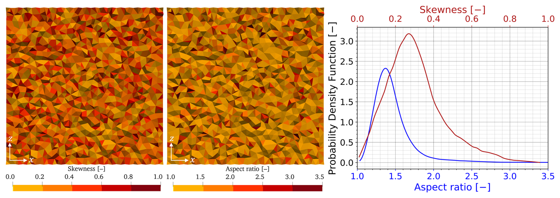
Figure 11 From left to right: x−z skewness plane at y=200 m, x−z aspect ratio planes at y=200 m, probability density function (PDF) of the skewness, and the aspect ratio distribution for the U3 mesh.

In summary, both structured and unstructured grids accurately reproduce the SBL structure and yield physically consistent representations of the flow of the GABLS1 case. Quantities such as friction velocity, velocity and temperature profiles, variances, and fluxes remain within the intercomparison ensemble spread. Nonetheless, systematic differences appear between the two grid types, particularly in wall heat flux, velocity variance, and flux magnitude. The enhanced turbulence level of the unstructured-grid simulation can primarily be attributed to differences in near-wall flux estimation, leading to higher friction velocities and thus stronger fluctuations produced near the wall. Nevertheless, the proper overall agreement supports the use of unstructured meshes for atmospheric LES in the wind energy context.

4.2.2 Sensitivity to resolution

Following the comparison of structured and unstructured meshes at the recommended resolution, we now investigate the influence of grid resolution on the simulation results. A sensitivity study is conducted with mesh sizes ranging from Δx=12.5 m to Δx=2 m. Simulations are labelled S1 to S4 and U1 to U4 for structured and unstructured grids, respectively, with the increasing index indicating higher resolution, as listed in Table 3.

Figure 12 Friction velocity, wall heat flux, and Monin–Obukhov length time series.

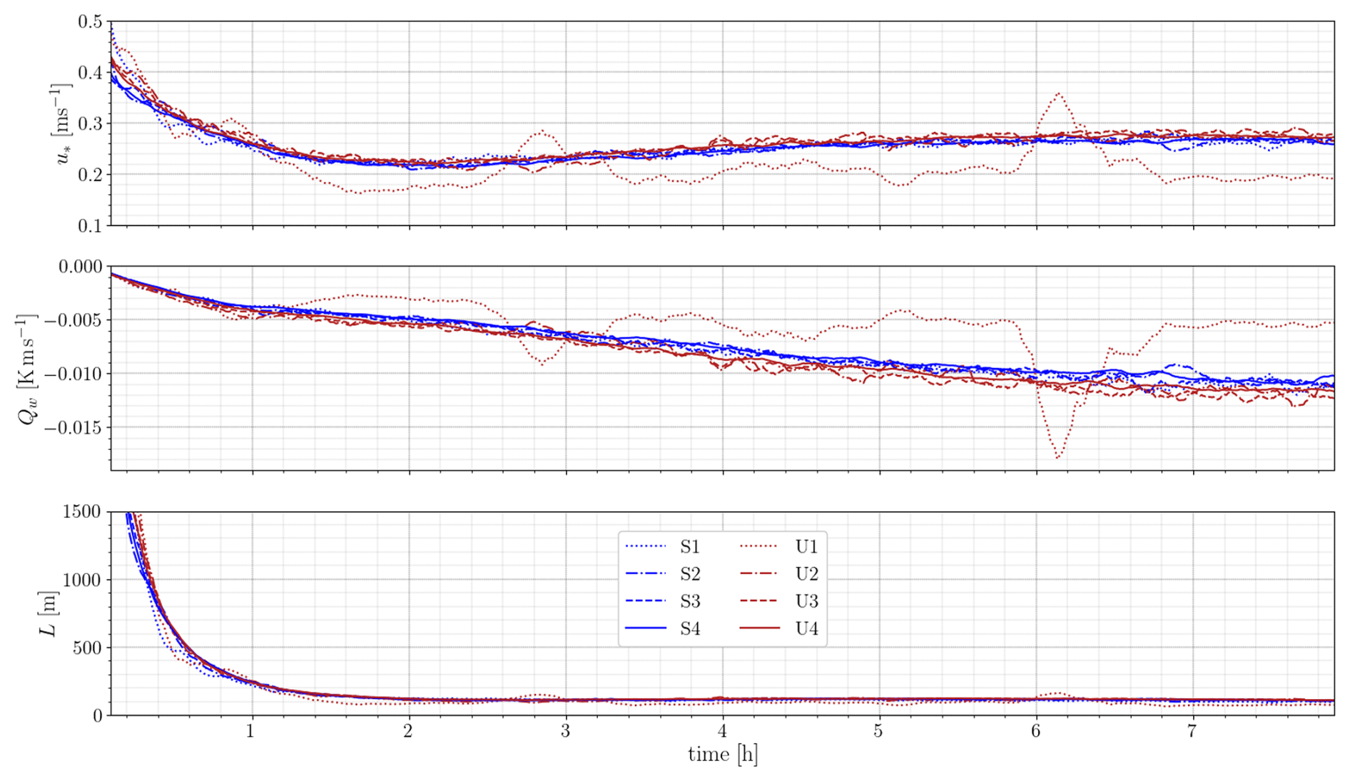
Time series of surface-integrated quantities are shown in Fig. 12. All simulations exhibit similar trends, with the exception of U1, which produces unreliable results. The friction velocity time series for structured grids is slightly lower and exhibits more noise. More significant differences are observed in the wall heat flux, which is consistently higher for unstructured-grid simulations. These differences influence the resulting temperature, velocity, and flux profiles discussed in Sect. 4.2.1. However, as the mesh is refined, results from both grid types converge, though not identically. Using finer resolutions reduces numerical diffusion and enables improved gradient capture. This supports the hypothesis that the discrepancy between grid types arises primarily from resolution-driven numerical effects. For the Monin–Obukhov length – a global measure of stability – all simulations converge closely.

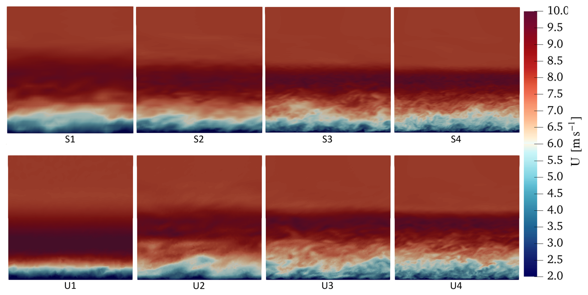
Figure 13 x−z velocity planes at y=200 m. Top: structured cases, bottom: unstructured cases. Mesh resolution increases from left to right.

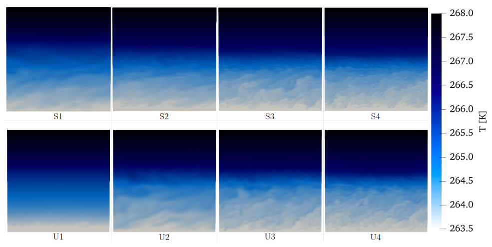
Figure 14 x−z temperature planes at y=200 m. Top: structured cases, bottom: unstructured cases. Mesh resolution increases from left to right.

Figures 13 and 14 provide a qualitative illustration of flow structures across resolutions. Both figures show instantaneous velocity and temperature fields in planes perpendicular to the y axis. As expected, mesh refinement reveals progressively finer-scale turbulent structures. While the resolution level has a visible impact, differences between structured and unstructured grids are not apparent at first glance.

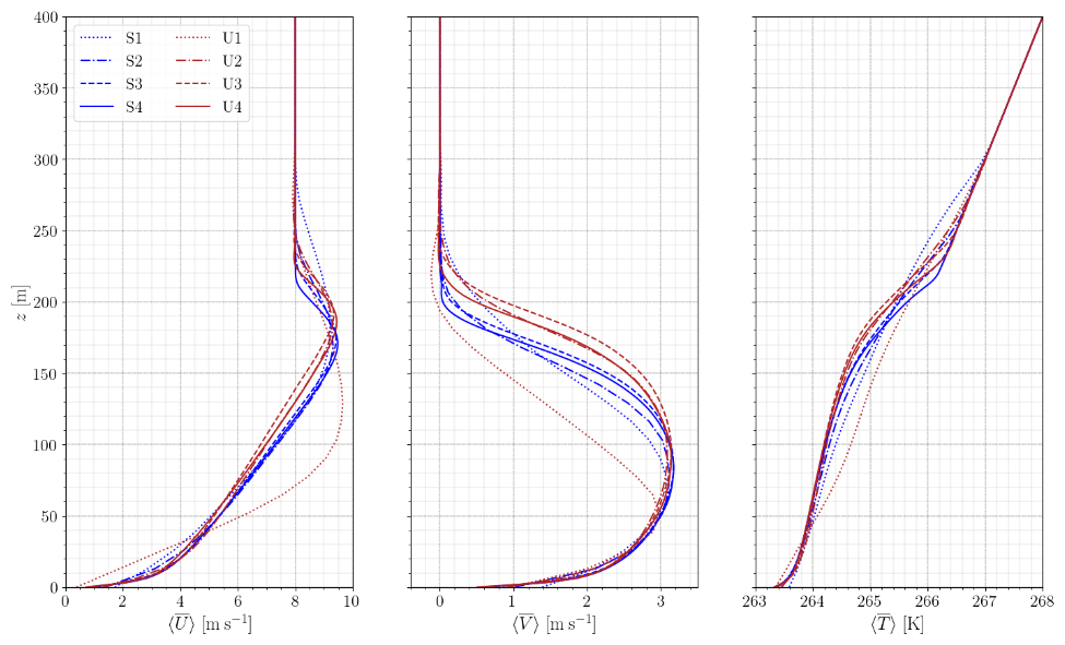
Figure 15 Time-averaged and horizontally averaged streamwise velocity, tangential velocity, and temperature profiles.

Horizontally and temporally averaged profiles between the 7th and 8th simulation hour are shown in Fig. 15. Except for U1, all cases follow similar trends. The temperature inflection point for unstructured grids consistently lies above that of the structured grids, confirming observations from Sect. 4.2.1. Velocity components tend to return to geostrophic values aloft.

Figure 16 Time-averaged and horizontally averaged momentum and heat flux profiles.

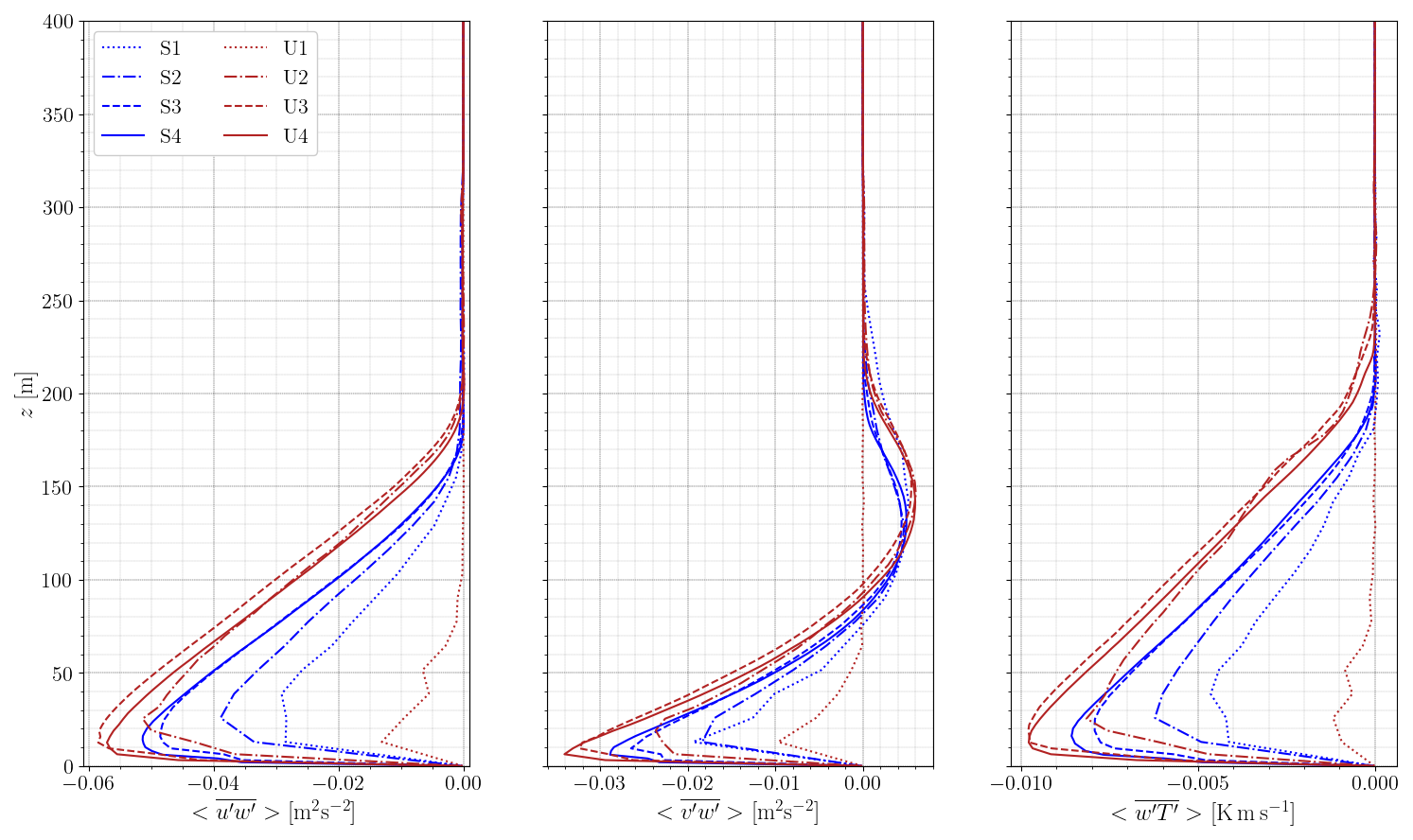
Figure 16 displays momentum and heat flux profiles. For all but the coarsest mesh, unstructured grids yield stronger fluxes throughout the boundary layer. At the coarsest resolution, fluxes are weak or vanish, indicating poor boundary layer representation. Finer meshes lead to stronger turbulent fluctuations, as expected from reduced numerical dissipation. These stronger fluxes correlate with the enhanced wall heat flux observed in unstructured simulations. Overall, except for the U1 and S1 cases, all other simulations produce satisfactory results. The coarse resolution in these two cases leads to unrealistic boundary layer development and are therefore excluded from further analysis.

To further assess simulation quality, the boundary layer height is computed following the approach proposed in Kosović and Curry (2000), based on the vertical distribution of turbulent stress. The SBL height is defined as the altitude where the tangential turbulent stress drops to α=5 % of its surface value. A linear extrapolation is applied:

$$\begin{array}{}\text{(9)}& h={\displaystyle \frac{z{\mathrm{|}}_{\langle \stackrel{\mathrm{‾}}{u^{\prime }{w}^{\prime }}\rangle =\mathit{\alpha }{u}_{*}^{\mathrm{2}}}}{\mathrm{1}-\mathit{\alpha }}}.\end{array}$$

Table 4 reports SBL heights from the present work and prior studies. Across all cases, boundary layer height decreases with increasing resolution, converging around 160–175 m. Unstructured-grid simulations yield SBL heights that are about 10 % higher, consistent with their stronger surface heat flux and momentum fluxes (Fig. 16).

(Beare et al., 2006)Cuxart et al. (2006)Stoll and Porté-Agel (2008)Huang and Bou-Zeid (2013)Abkar and Moin (2017)Gadde et al. (2021)Min and Tombouldies (2022)

Table 4 Boundary layer heights in various studies, depending on the grid resolution.

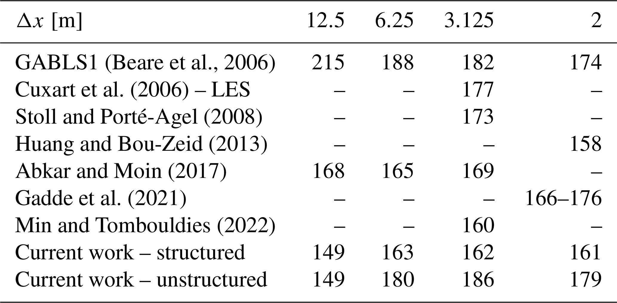
The original GABLS1 study used Δx=1 m as a reference, yielding an SBL height of 157 m. Simulations within 20 % of this value are considered acceptable (Beare et al., 2006). By this standard, all simulations with Δx≤6.25 m are accurate, with deviations between 3.8 % and 1.9 % for structured grids and 18 % and 14 % for unstructured grids.

Table 5 Relative L₂ norm error in percent of the horizontal average velocity and temperature profiles compared to the reference profiles from Beare et al. (2006).

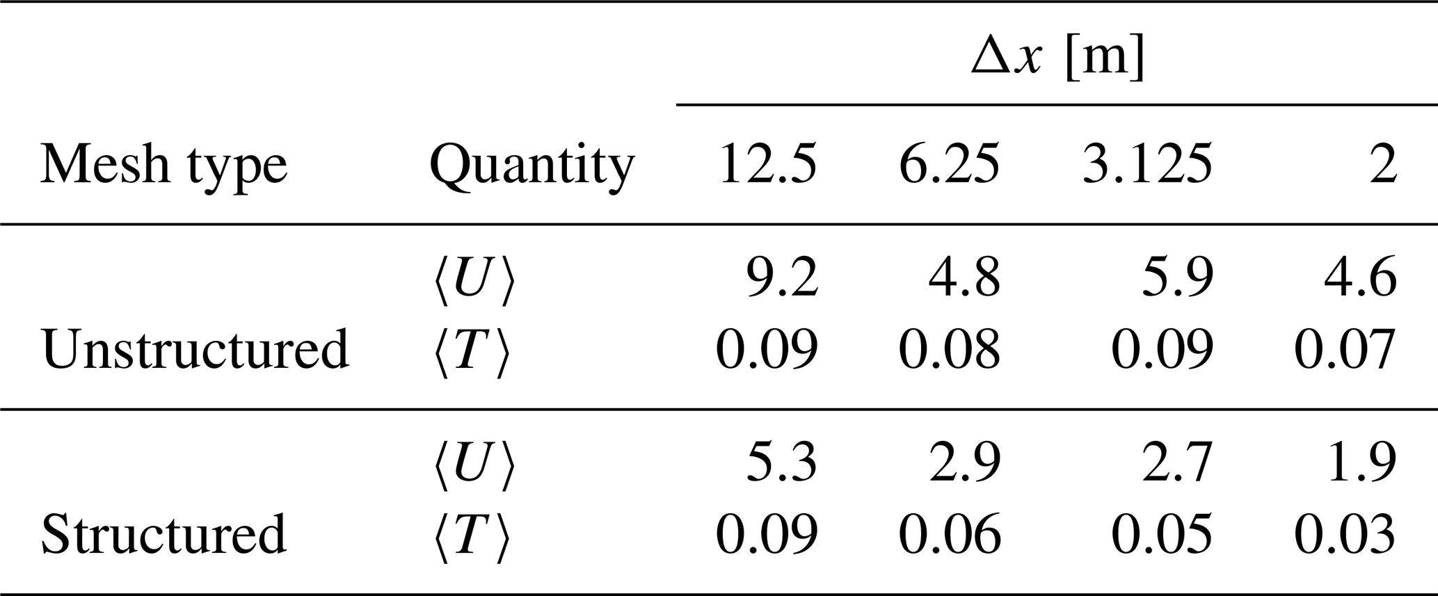
To complement this analysis, the relative L₂ norm error is computed between horizontal average profiles from the present work and the reference profiles in Beare et al. (2006). Results are summarized in Table 5. Excluding the coarsest cases, velocity profile errors remain below 6 % and temperature profile errors below 0.1 %. Grid convergence appears below Δx=6.25 m, with structured grids exhibiting slightly better agreement overall.

5 Conclusions

This study presents a high-order incompressible Navier–Stokes solver capable of performing large-eddy simulations of the stable atmospheric boundary layer on unstructured meshes – a significant step forward, given the complexity of such simulations. The solver incorporates the Coriolis force, the Boussinesq approximation for buoyancy effects, and wall modelling via Monin–Obukhov similarity theory.

The framework was first validated against the Andren benchmark, comparing mean profiles, variances, friction velocity, and vertical momentum flux with previous studies. Simulations on both structured and unstructured grids produced similar results, with only minor discrepancies. The unstructured grid slightly overestimated friction velocity and velocity variance, primarily due to lower mesh quality near the wall and associated wall gradient reconstruction. However, its influence was found to be less significant than that of the numerical solver choices.

The solver was then evaluated using the well-established GABLS1 benchmark. LES using both grid types at a recommended resolution of Δx=3.125 m reproduced the main features of the SBL with very good agreement compared to both the original study and more recent studies. As with the neutral case, gradient estimation proved marginally less accurate in unstructured grids. This led to subtle differences in flux prediction and SBL evolution, with the boundary layer height in unstructured grids approximately 10 % higher, along with stronger momentum and heat fluxes. Nonetheless, these differences remain within the range of variability observed across other LES studies in the literature. Overall, subgrid-scale modelling, numerical schemes, and grid resolution were found to have a more pronounced influence on the results than mesh structure.

A resolution sensitivity analysis further demonstrated that a grid spacing of Δx=6.25 m is sufficient to achieve boundary layer height predictions within 20 % of a high-resolution reference. The relative L₂ norm errors for horizontal velocity and temperature profiles remained below 6 % for both mesh types, with errors decreasing as resolution improved. These findings indicate that both structured and unstructured grids can provide robust and accurate LES of the SBL, particularly at Δx=3.125 m resolution. Concerning the computational performance, an overcost of 14 % is measured for the U3 mesh case compared to the S3 one. This noticeable increase has been evaluated on a simple bi-periodic 3D box configuration. For more realistic applications with complex topography, the comparison is not relevant since a body-fitted structured-mesh approach cannot be used.

To the best of the authors' knowledge, this work represents one of the first successful LESs of the stable boundary layer using unstructured grids. This new approach of high-fidelity simulations over geometrically complex terrain overcomes the limitations imposed by structured meshes. Future work will focus on extending this framework to realistic applications in wind energy and atmospheric science.

Appendix A: GABLS1 source of errors

Two sources of debate can be highlighted in the design of the GABLS1 benchmark (Beare et al., 2006): initial condition definition and numerical error accumulation.

A1 Initial condition definition

The initial condition of the vertical temperature profile of the GABLS1 benchmark is spatially uniform, set to T=265 K from the ground up to z=100 m, and then increases by $\mathrm{1}\mathrm{K}/\mathrm{100}\mathrm{m}$. To help the flow destabilization process, a random potential temperature perturbation of 0.1 K amplitude is superposed to the profile between z=0 m and z=50 m. The definition of this random perturbation is left to the user's discretion, which is questionable. Commonly, users add randomly generated noise that is spatially uncorrelated on each control volume. This can clearly have an impact on the flow evolution and will depend on the mesh resolution and grid partitioning.

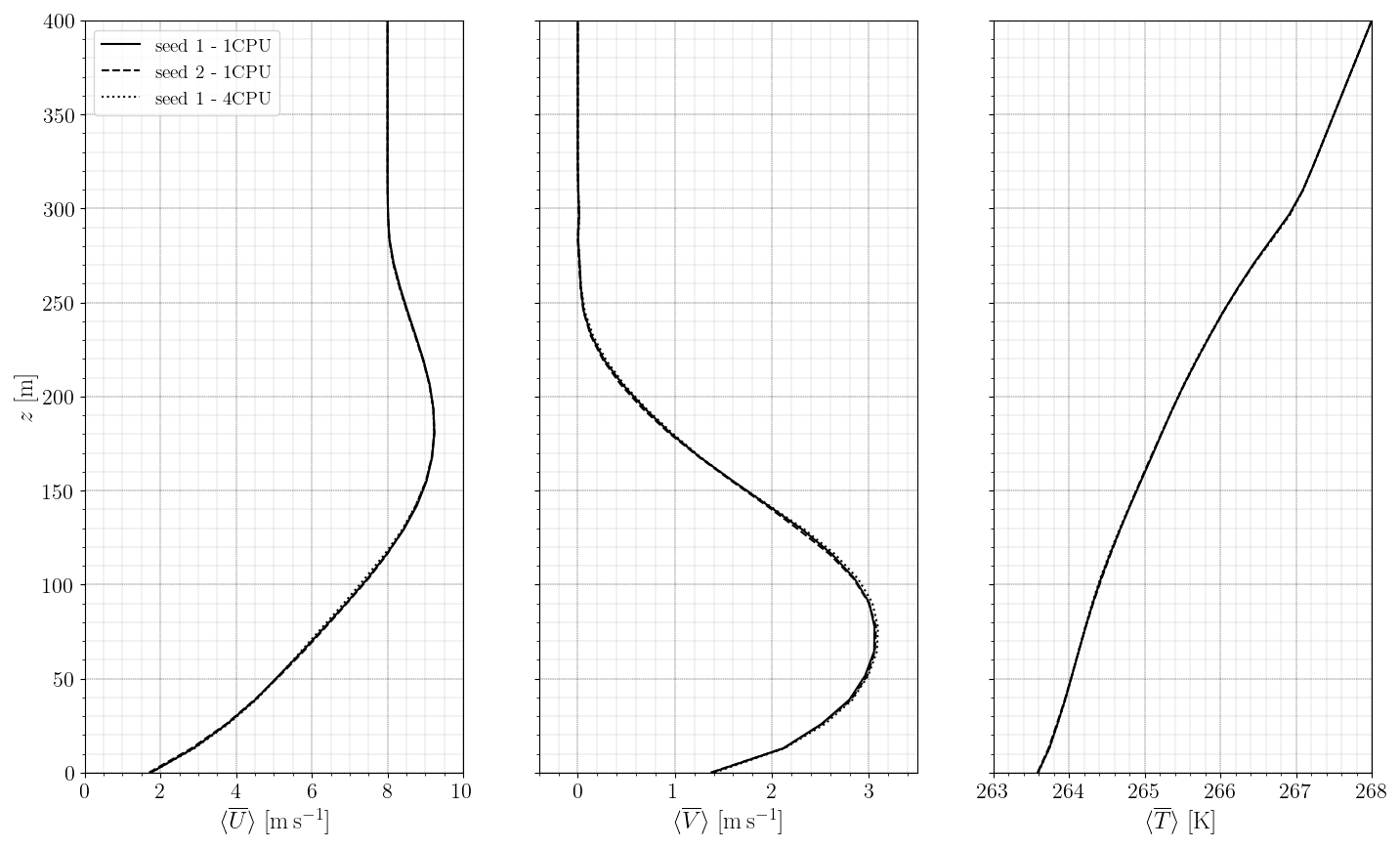
Figure A1 Time-averaged and horizontally averaged streamwise velocity, tangential velocity, and temperature profiles on the S1 mesh. Results with seed 1 and 1 CPU core (solid black line), seed 2 and 1 CPU core (dashed black line), and seed 1 and 4 CPU cores (dotted black line).

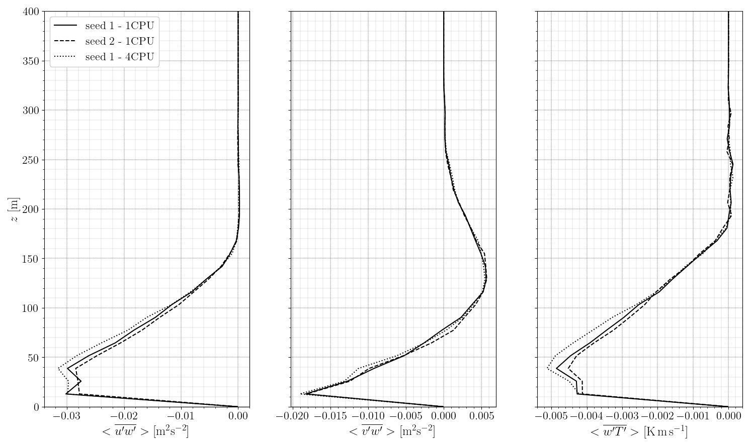
Figure A2 Time-averaged and horizontally-averaged momentum and heat flux profiles on the S1 mesh. Results with seed 1 and 1 CPU core (solid black line), seed 2 and 1 CPU core (dashed black line), and seed 1 and 4 CPU cores (dotted black line).

To quantify its impact on the flow behaviour, two identical simulations based on the Δx=12.5 m structured grid (S1) are performed, with the only difference being the random number seeds. Figure A1 shows the streamwise velocity, tangential velocity, and temperature profiles spatially averaged over horizontal planes and temporally averaged between the 7th and the 8th hour, thus long after initialization. This figure highlights no visible differences. Simulations with different seeds exhibit similar velocity and temperature profiles, at least when averaged over space and time. However, Fig. A2, displaying the time- and space-averaged momentum and heat flux profiles, shows otherwise. Deviations are larger within the stable boundary layer. Differences in heat flux are of the order of 5 % with a maximum of 8 % at z=40 m. Although not huge, the results show a clear dependence of the flow on the random seed. It is important to remember that these results are averaged spatially across the entire domain and temporally over 1 h. Thus, a measurable difference implies a difference in flow dynamics. These results are reproducible for different grid resolutions and numerical schemes but are not shown here for the sake of clarity.

This effect means that a small change in the initial profile affects the behaviour of the flow and thus the collected statistics. It can distort the comparison between codes since the random number generation will necessarily be different. Moreover, this random number is only determined by an amplitude and a mean, analogous to white noise without spatial coherence. As different grid resolutions were used in all GABLS1 studies, different fluctuation frequencies were added. Since the flow behaviour is sensitive to this initial profile, part of the differences obtained when comparing two resolutions can be explained by this phenomenon. Similarly, it could also explain differences between structured and unstructured grids. Adding constraints on the random number, such as specifying the fluctuation frequency or some spatial correlation, would help ensure similar initial conditions, regardless of the mesh type or the resolution. The perturbation would then be analogous to pink noise instead of white noise. The results would still depend on the random number seed but would at least minimize differences when comparing different resolutions.

A2 Numerical error accumulation

Theoretically, a deterministic simulation behaviour is expected, since the resolution of the Navier–Stokes equations is fully deterministic. Simulations are reproducible, and all states can be derived from the input data. However, numerical errors can lead to non-deterministic flows; i.e. different results can be obtained with identical input data. The sources of numerical errors are numerous: node reordering, machine precision, operation orders, etc. In this respect, the grid partitioning and therefore number of CPU cores used in a LES can cause variations in the results. It has been demonstrated that the propagation of numerical errors is linear for laminar flows but exponential for turbulent flows (Marta, 2009). This difference between laminar and turbulent flows is due to the true chaotic nature of turbulence.

To illustrate this effect, two identical simulations were performed on the Δx=12.5 m structured grid (S1) with different numbers of CPU cores: one simulation with 1 CPU and the other with 4 CPUs and by keening the same random generator seed. Again, Fig. A1, which displays the streamwise velocity, tangential velocity, and temperature profiles, shows no visible differences. Yet, Fig. A2, which displays the momentum and heat flux profiles, shows discrepancies depending on the number of CPUs used. Deviations are larger within the stable boundary layer. Differences in heat flux are of the order of 10 % with a maximum of 15 % at z=40 m. Similar gaps are observed for other grid resolutions and numerical schemes but are not shown for the sake of brevity. As the errors accumulate quickly, working with higher machine precision will not suppress the error propagation but only delay it. Since error propagation is exponential, the flow paths will always diverge (Marta, 2009). To circumvent this effect, several simulations with different random number generations could be performed and averaged to give more statistical accuracy.