Dual-lidar profilers for measuring atmospheric turbulence

A dual-lidar system comprising two WindCube v2.1 Doppler lidars – one oriented horizontally at a 45° angle relative to the other – was deployed to estimate atmospheric turbulence using the variance method. This approach derives second-order velocity statistics directly from line-of-sight (LOS) velocity variances, enabling the reconstruction of the three-dimensional velocity variance components without retrieving instantaneous wind vectors. Its performance is evaluated against the traditional method commonly used in the wind energy sector, which reconstructs instantaneous velocity components from single-lidar LOS measurements prior to computing turbulence statistics. Both methods are assessed at a single measurement height using a 30 d collocated dataset, with sonic anemometer measurements as reference and classification by atmospheric stability. The analysis focuses on turbulence intensity (TI), and performance is quantified using the mean relative bias error (MRBE) and relative root mean square error (RRMSE), following Det Norske Veritas (DNV) load-validation acceptance criteria (MRBE within ±5 % and RRMSE ≤ 15 %). Results show that the variance method demonstrates improved agreement with the reference measurements across nearly all wind-speed bins. For along-wind TI, MRBE values range between 0 % and −5 %, with RRMSE remaining below 15 % over the full wind-speed range, fully satisfying the DNV criteria. For cross-wind TI, the MRBE criterion is met, while the RRMSE threshold is exceeded. In contrast, the traditional method meets both DNV criteria for along-wind TI only at wind speeds above approximately 7 m s⁻¹ and fails to satisfy either criterion for cross-wind TI across the investigated range. Overall, the results demonstrate that the variance method provides more robust and DNV-compliant TI estimates than the traditional reconstruction approach, particularly for along-wind turbulence relevant to wind turbine load validation.

1 Introduction

In recent years, wind lidar profiler technology has increasingly replaced traditional meteorological masts equipped with in situ sensors such as cup or sonic anemometers for measuring key mean wind properties like speed and direction. Wind lidars can be broadly categorized based on their emission waveform (pulsed or continuous) and their associated measurement techniques. Pulsed lidar profilers commonly employ the Doppler beam swinging (DBS) technique (Strauch et al., 1984), in which line-of-sight (LOS) velocities are sampled sequentially along several fixed beam directions. Velocity–azimuth display (VAD) scanning (Browning and Wexler, 1968) is also widely applied with pulsed lidars, as well as with continuous-wave systems, and is frequently used for turbulence retrievals (e.g., Mann et al., 2010).

Lidar profilers offer clear advantages for characterizing mean wind properties, including reduced deployment costs and the ability to measure at similar or greater heights above the ground compared to meteorological masts. However, wind lidar profilers have not yet gained widespread acceptance for turbulence measurements, which remain an active area of research. In contrast to reference instruments such as cup or sonic anemometers, turbulence estimates from lidar profilers are affected by systematic errors arising from three main sources: (i) inter-beam effects, (ii) intra-beam averaging, and (iii) instrumental noise.

Inter-beam effects can lead to the over- or underestimation of turbulence metrics through wavenumber-dependent modulation of turbulent energy when LOS measurements from spatially separated beams are combined (Theriault, 1986; Gargett et al., 2009; Kelberlau and Mann, 2020). This effect is closely linked to violations of the assumption of instantaneous spatial homogeneity inherent to multi-beam techniques. Intra-beam effects arise from probe-volume and probe-time averaging, and lead to an underestimation of turbulent energy due to spatial and temporal filtering of velocity fluctuations (Thiébaut et al., 2025). Instrumental noise introduces an additional variance contribution to LOS velocity measurements and can therefore bias turbulence estimates if not properly accounted for.

Turbulence intensity (TI) is a key metric in wind energy for assessing turbine loads, site suitability, and energy yield. The traditional approach estimates TI from second-order statistics of reconstructed velocity components using LOS measurements from a single-lidar profiler. This reconstruction combines inter-beam coupling, intra-beam averaging, and instrumental noise effects, which may partially compensate and lead to apparently accurate TI estimates for the wrong reasons (Kelberlau and Mann, 2019).

An alternative class of approaches derives turbulence statistics directly from LOS velocity variances or Doppler spectral information. Eberhard et al. (1989) showed that turbulence kinetic energy and velocity covariances can be retrieved from a full VAD scan at an elevation angle of 35.3°, provided sufficient azimuthal sampling. Later studies demonstrated that VAD-based methods can yield accurate turbulence statistics when intra-beam averaging effects are explicitly corrected (e.g., Smalikho and Banakh, 2017; Wildmann et al., 2020; Päschke and Detring, 2024).

Similar concepts have been applied to pulsed Doppler lidar profilers operating in DBS configurations, where second-order statistics are inferred directly from LOS velocity variances. However, standard five-beam DBS geometries (one vertical and four slanted beams) cannot resolve the horizontal cross-term variance σ_xy (here defined in the lidar instrument-fixed horizontal coordinate system x–y), preventing a full rotation into the streamwise coordinate system. As a result, these approaches are generally applicable only when the mean wind direction is aligned with a pair of opposing slanted beams (e.g., Thiébaut et al., 2024). Resolving σ_xy requires an additional slanted beam. Sathe et al. (2015) demonstrated this using a six-beam ground-based scanning pulsed lidar (WindScanner), enabling TI estimation from second-order statistics of the full three-dimensional velocity field and validation against VAD-based lidar and cup anemometer measurements. Recently, this concept has been transferred to commercial instrumentation with the release of the BEAM6x WindPower lidar profiler from Lumibird, inspired by the WindScanner architecture; however, as a newly introduced system, its performance and suitability for routine turbulence characterization are not yet well established.

In oceanographic studies, acoustic Doppler current profilers (ADCPs) are widely used to derive first- and second-order flow statistics. ADCPs are Doppler-based remote sensing instruments that employ multiple acoustic beams to measure water velocity. A common configuration is the Janus geometry, exemplified by the Teledyne RDI Workhorse Sentinel, which uses four beams inclined 20° from the vertical. Similar multi-beam concepts are used in atmospheric lidar systems: the WindCube v1 employed a comparable configuration with steeper beam angles, while modern ADCPs such as the Nortek Signature series use a five-beam Janus setup with four beams at 25° and one vertical beam. This closely resembles the WindCube v2.1 configuration, which combines four beams inclined at α=28° with a vertical beam. ADCPs may be deployed either bottom-mounted in an upward-looking configuration (e.g., Thomson et al., 2012; McMillan et al., 2016; Thiébaut et al., 2022) or downward-looking when installed on floating platforms or vessels (e.g., Goddijn-Murphy et al., 2013; Sentchev et al., 2019; Thiébaut et al., 2019).

The method based on second-order statistics of LOS velocity measurements to reconstruct three-dimensional velocity variances is well established in oceanography and is commonly referred to as the variance method (e.g., Stacey et al., 1999a; Lu and Lueck, 1999; Rippeth et al., 2002). Turbulence analysis using a single ADCP (up to five beams) typically relies on assumed turbulence anisotropy ratios, often derived from laboratory experiments (e.g., Stacey et al., 1999b; Lueck et al., 2002; Peters and Johns, 2006). However, such assumptions can introduce substantial uncertainty. Burchard et al. (2008) demonstrated that the difference between isotropic and fully anisotropic turbulence may lead to up to a sixfold error in turbulent kinetic energy (TKE) estimates from a four-beam ADCP. These assumptions are unavoidable because fewer than six independent beams cannot resolve all components of the Reynolds stress tensor.

To address this limitation, Vermeulen et al. (2011) proposed a dual-ADCP configuration combining two four-beam RDI instruments with a 45° relative heading offset, forming an eight-beam system. This orientation was shown numerically to minimize variance-estimation errors. One instrument was additionally pitched by 20°, aligning one beam vertically and enabling direct measurement of the vertical velocity component. With eight independent beams, the full Reynolds stress tensor can be resolved without invoking anisotropy assumptions and rotated into any desired coordinate frame. This approach was later implemented by Thiébaut et al. (2020) to investigate the TKE budget in the Alderney Race tidal channel and was further validated using large-eddy simulations by Mercier et al. (2021).

Building on the methodology introduced by Vermeulen et al. (2011) for ADCPs, we developed a modified version tailored to dual-WindCube v2.1 lidar profilers. This configuration provides the minimum number of independent beams required by the variance method using well-established commercial lidar profilers as an alternative to recently commercialized six-beam lidar profilers. The method is benchmarked against the traditional approach used in the wind power industry. Both methods are evaluated at a single altitude using a 30 d collocated dataset, with reference measurements from a three-dimensional sonic anemometer classified by atmospheric stability conditions. Two key performance metrics are considered: the mean relative bias error (MRBE) and the relative root mean square error (RRMSE), as defined by DNV (Det Norske Veritas) (DNV, 2023).

The remainder of this paper is organized as follows. The study begins with a description of the study site (Sect. 2.1), instrumentation (Sect. 2.2), and data selection (Sect. 2.3), along with methods for instrumental noise correction and spike filtering (Sect. 2.4 and 2.5). This section also presents the traditional method for single-lidar profilers, the variance method for dual-lidar profilers, and the reference sonic anemometer measurements used to derive TI (Sect. 2.6) and velocity spectra (Sect. 2.7). Atmospheric stability classification based on the sonic anemometer measurements is described in Sect. 2.8. Error metrics for method evaluation are defined in Sect. 2.9. The results of the comparative analysis between the variance and traditional methods are presented in Sect. 3, followed by a discussion in Sect. 4. Finally, Sect. 5 summarizes the main findings and provides concluding remarks.

2 Data and methods

2.1 Study site and meteorological mast

The measurement mast is located approximately 13 km offshore from Fécamp, along the coast of Normandy, France (Fig. 1). It was originally installed for wind farm site characterization and is now operated by France Énergies Marines. The mast is situated within the offshore wind farm area, with the nearest turbine located approximately 400 m to the west. The site is characterized by strong tidal conditions, with a mean tidal range of about 8.8 m, and represents a typical offshore environment for wind energy applications.

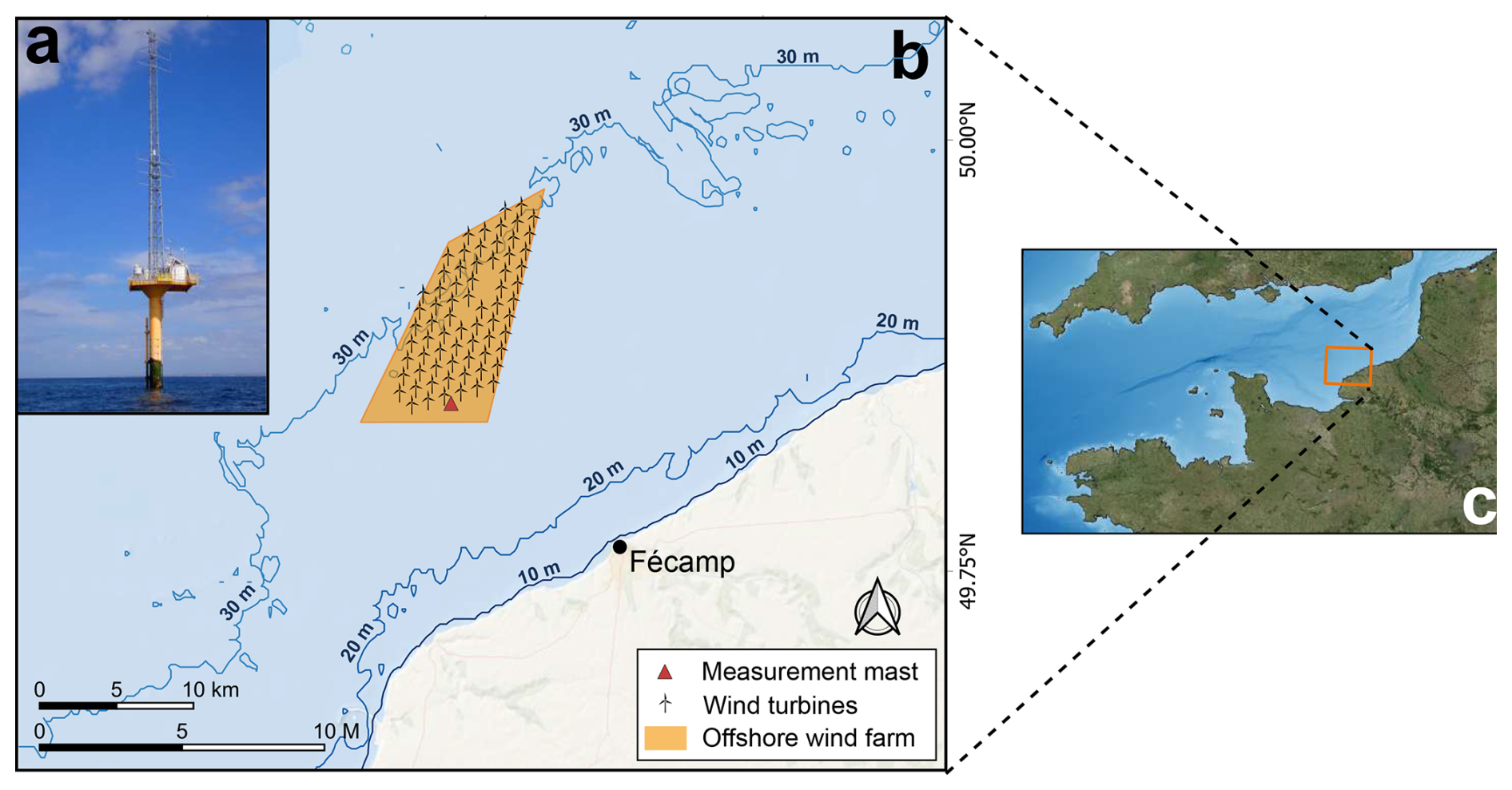
Figure 1 Photograph of the measurement mast (a), located 13 km off the coast of Fécamp, situated in front of the first row of wind turbines in the offshore wind farm (b), which is deployed off the coast of Normandy, France (c).

All results presented in this study are based on measurements at 40 m above the mast platform. Fig. 2 summarizes the mean wind conditions observed during the 30 d analysis period at this measurement height. The mean wind speed was 8.5 m s⁻¹, with a maximum observed value of 21.0 m s⁻¹. The wind direction distribution is dominated by south-westerly flows, with a mean wind direction of approximately 205° and a directional spread of about 74°. These conditions are representative of an offshore wind regime and provide a broad range of wind speeds and directions for the evaluation of the lidar-based turbulence retrieval methods.

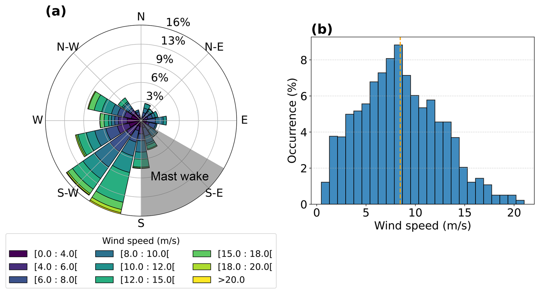
Figure 2 Wind statistics measured at 40 m above the mast platform at the measurement site. (a) Wind rose for the analysis period. The shaded gray sector indicates wind directions affected by mast wake excluded from the analysis. (b) Histogram of wind speed occurrence. The vertical orange line indicates the mean wind speed.

2.2 Sensors equipment

The measurement mast is equipped with a three-dimensional THIES sonic anemometer mounted on a boom at a height of 39 m above the platform (Fig. 3a). The measurement volume of the sonic anemometer is positioned at 39.5 m, as it is located 0.5 m from the tip of the boom. The boom is oriented at an angle of −60° from true north (Fig. 3b). The anemometer is aligned such that the x-axis points toward true north, the y axis toward the west, and the z axis vertically upward. The (x, y, z) coordinate system associated with the sonic anemometer served as the reference coordinate system in this study. The anemometer collects wind velocity data at an acquisition rate of 10 Hz.

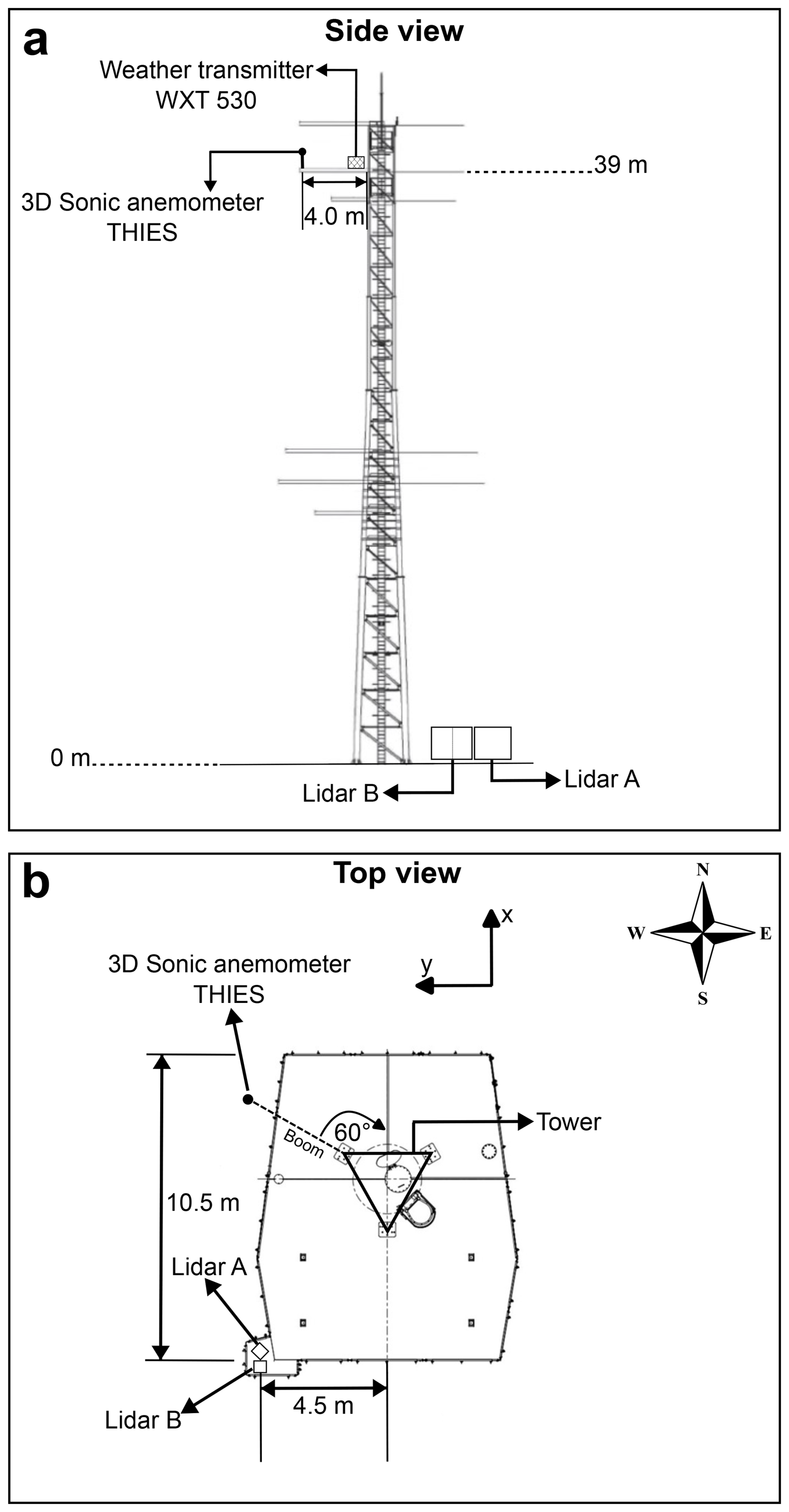
Figure 3 Side view (a) and top view (b) schematics of the 40 m measurement mast, detailing the deployed sensors and their positions on the mast and platform.

To complement this setup, two Vaisala offshore WindCube v2.1 lidar profilers were installed at the platform level (Figs. 3b and 4b, c). The primary lidar, referred to as lidar A, was oriented in such a way that beams one and three – aligned with the x axis of the instrument's coordinate system – were directed toward true north, while beams two and four were aligned with the y axis. The fifth beam of lidar A pointed vertically along the z axis. Note that the manufacturer configured the z axis of the lidar to point vertically downward. The secondary lidar, referred to as lidar B, was mounted adjacent to lidar A and rotated at θ= 45° in the horizontal plane relative to lidar A. Both lidars were installed with a tilt angle of less than 0.2°. Together, the two lidars formed a combined 10-beam scanning arrangement (Fig. 4a), enabling measurements of LOS velocities at 10 vertical levels ranging from 40 to 240 m above the platform. LOS velocity data were recorded at a sampling rate of 0.25 Hz. For consistency in the point-by-point comparison, the sonic anemometer time series was resampled to the same rate using a standard decimation procedure.

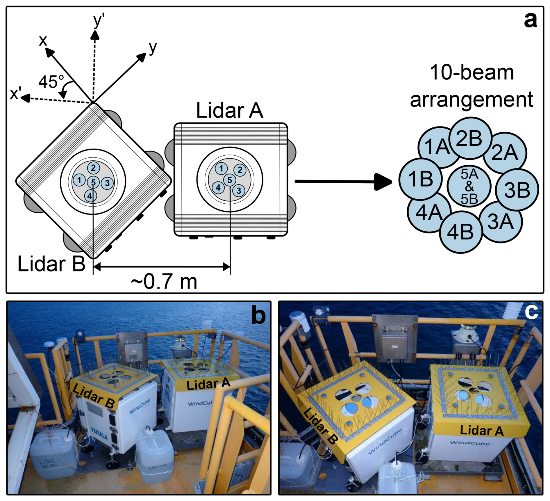
Figure 4 (a) Schematic of the 10-beam arrangement formed by combining the five beams of lidar A with the five beams of lidar B, which is rotated 45° relative to lidar A. (b) Side view and (c) top view photographs of the setup installed at the platform level.

Additionally, atmospheric data are collected by a Vaisala WXT 530 weather transmitter, installed on the mast at a height of 39 m above the platform. This sensor provides 10 min averaged values of pressure, temperature, and humidity.

2.3 Data selection

A 30 d dataset, spanning from 1 April to 1 May 2024, was compiled for turbulence analysis. This dataset was divided into 1440 non-overlapping 30 min ensembles. The choice of a 30 min averaging window, rather than the 10 min interval commonly used in wind energy practice and in DNV error metrics, was made deliberately to reduce random errors in turbulence statistics. Longer averaging periods improve statistical convergence of second-order moments, as discussed by Lenschow et al. (1994), and are therefore better suited for the present turbulence analysis. The analysis focused on wind speeds exceeding 3 m s⁻¹, corresponding to the typical cut-in speed of most wind turbines. Applying this threshold led to the exclusion of approximately 6 % of the original dataset. Additionally, wind measurements associated with wind directions between 120 and 180° (relative to true north) were excluded to avoid contamination from mast wake effects affecting the sonic anemometer data (Fig. 2a). This directional filtering removed a further 11 % of the remaining ensembles. To ensure data quality, any 30 min ensemble containing less than 90 % valid velocity measurements was also discarded, resulting in an additional 9 % reduction. Individual velocity measurements were considered valid only if their carrier-to-noise ratio (CNR), provided by the lidar systems, was greater than −23 dB, as recommended by the manufacturer. After applying all filtering criteria, a total of N= 1098 30 min ensembles were retained for turbulence analysis.

2.4 Instrumental noise

Lidar measurements are inherently influenced by signal noise and by small variations in aerosol gravitational settling velocities, which – although weak – can contribute additional terms to the observed variance. Assuming that all atmospheric flow contributions to the observed LOS velocity variance within the considered short timescales are of a turbulent nature, the variance ${\mathit{\sigma }}_{b_i}^{\mathrm{2}}$ of the LOS velocity measured by beam i can be expressed as the sum of three independent terms (Doviak and Zrnic, 1993):

$$\begin{array}{}\text{(1)}& {\mathit{\sigma }}_{b_i}^{\mathrm{2}}={\mathit{\sigma }}_{p_i}^{\mathrm{2}}+{\mathit{\sigma }}_{n_i}^{\mathrm{2}}+{\mathit{\sigma }}_{d_i}^{\mathrm{2}}.\end{array}$$

Here, ${\mathit{\sigma }}_{p_i}^{\mathrm{2}}$ represents the net contribution from atmospheric turbulence at scales measurable by the lidar (Brugger et al., 2016), ${\mathit{\sigma }}_{n_i}^{\mathrm{2}}$ denotes the variance associated with instrumental noise, and ${\mathit{\sigma }}_{d_i}^{\mathrm{2}}$ accounts for the variance caused by variations in aerosol terminal fall speeds within the probe volume. However, ${\mathit{\sigma }}_{d_i}^{\mathrm{2}}$ can typically be neglected, as particle fall speeds are generally less than 1 cm s⁻¹ (e.g., Bodini et al., 2018).

The noise contribution ${\mathit{\sigma }}_{n_i}^{\mathrm{2}}$ is often quantified through an autocorrelation approach. In this method, the temporal autocorrelation function of the measured LOS velocity time series

$$\begin{array}{}\text{(2)}& R\left(\mathit{\tau }\right)={\displaystyle \frac{\langle b_i\left(t\right)b_i(t+\mathit{\tau })\rangle }{{\mathit{\sigma }}_{b_i}^{\mathrm{2}}}}\end{array}$$

is examined at short time lags τ. While atmospheric fluctuations remain correlated over small τ, the noise component is uncorrelated and manifests as a discontinuity at the first non-zero lag. The reduction of R(τ) between τ=0 and τ=Δt can therefore be used to estimate ${\mathit{\sigma }}_{n_i}^{\mathrm{2}}$ (e.g., Mayor et al., 1997; Lenschow et al., 2000). For a wind lidar profiler such as the WindCube v2.1, the sampling interval Δt corresponds to the accumulation time of the Doppler signal at one LOS position. This separation enables the retrieval of the turbulence-related variance ${\mathit{\sigma }}_{p_i}^{\mathrm{2}}$ with reduced contamination from instrumental effects. Note that, for consistency, instrumental noise was similarly removed from variance of the time series of the instantaneous reconstructed horizontal velocities, u_x and u_y, employed in the traditional method (Sect. 2.6.2).

2.5 Spike filtering

To remove spurious outliers in the velocity measurements, a spike-filtering procedure following Wang et al. (2015) was applied. The method was implemented over consecutive 30 min windows and is based on the analysis of differences between adjacent velocity samples. A data point was flagged as a spike when the absolute differences at two consecutive time steps exceeded twice the interquartile range (IQR) of the local difference distribution and exhibited opposite signs. Identified spikes were removed by setting the corresponding values to NaN (not a number). This filtering was applied consistently to all datasets, including lidar LOS velocities, reconstructed horizontal wind components, and sonic anemometer measurements.

2.6 Reconstruction of turbulence metrics

2.6.1 Sonic anemometer

To reduce the influence of alignment and tilt errors, the sonic anemometer data were processed using a standard double-rotation procedure (Kaimal and Finnigan, 1994; Foken and Mauder, 2008). First, the coordinate system was rotated in the horizontal plane to align the streamwise velocity component with the mean wind direction over each 30 min averaging period. A second rotation in the vertical plane was then applied to ensure zero mean vertical velocity. In the resulting coordinate system, the velocity components are denoted as u, v, and w, corresponding to the along-wind, cross-wind, and vertical components, respectively. The along- and cross-wind turbulence intensities TI_u and TI_v were computed as

$$\begin{array}{}\text{(3)}& {\displaystyle }{\mathrm{TI}}_u={\displaystyle \frac{{\mathit{\sigma }}_u}{U}}\text{(4)}& {\displaystyle }{\mathrm{TI}}_v={\displaystyle \frac{{\mathit{\sigma }}_v}{U}},\end{array}$$

where σ_u and σ_v are the standard deviations of u and v, and U is the mean horizontal wind speed defined as the temporal mean of $\sqrt{u^{\mathrm{2}}+v^{\mathrm{2}}}$.

2.6.2 Single-lidar profiler – Traditional method

For the traditional lidar-based approach, instantaneous horizontal velocity components were reconstructed from LOS measurements of a single-lidar profiler. The reconstructed velocities were rotated in the horizontal plane following the same procedure as for the sonic anemometer. Due to the small lidar tilt angles, no additional vertical rotation was applied. The resulting velocity components were used to compute the standard deviations ${\stackrel{\mathrm{̃}}{\mathit{\sigma }}}_u$ and ${\stackrel{\mathrm{̃}}{\mathit{\sigma }}}_v$, from which the corresponding turbulence intensities, denoted as ${\stackrel{\mathrm{̃}}{\mathrm{TI}}}_u$ and ${\stackrel{\mathrm{̃}}{\mathrm{TI}}}_v$, were derived following the definition given in Sect. 2.6.1.

2.6.3 Dual-lidar profilers – Variance method

The variance method involves the computation of second-order statistics of the three-dimensional velocity components from the LOS velocity variances. Building on the methodology introduced by Vermeulen et al. (2011) for ADCPs, we developed a modified version tailored to dual-WindCube v2.1 lidar profilers, each with a five-beam configuration. Our approach constructs a 10-element vector b containing noise-corrected LOS variances ${\mathit{\sigma }}_{p_i}^{\mathrm{2}}$ from both devices, allowing the reconstruction of the full Reynolds stress tensor. The vector is defined as

$$\begin{array}{}\text{(5)}& \begin{array}{rl}\mathit{b}& =[{\mathit{\sigma }}_{p_{\mathrm{1}},\mathrm{A}}^{\mathrm{2}},{\mathit{\sigma }}_{p_{\mathrm{2}},\mathrm{A}}^{\mathrm{2}},{\mathit{\sigma }}_{p_{\mathrm{3}},\mathrm{A}}^{\mathrm{2}},{\mathit{\sigma }}_{p_{\mathrm{4}},\mathrm{A}}^{\mathrm{2}},{\mathit{\sigma }}_{p_{\mathrm{5}},\mathrm{A}}^{\mathrm{2}},{\mathit{\sigma }}_{p_{\mathrm{1}},\mathrm{B}}^{\mathrm{2}},{\mathit{\sigma }}_{p_{\mathrm{2}},\mathrm{B}}^{\mathrm{2}},\\ & {\mathit{\sigma }}_{p_{\mathrm{3}},\mathrm{B}}^{\mathrm{2}},{\mathit{\sigma }}_{p_{\mathrm{4}},\mathrm{B}}^{\mathrm{2}},{\mathit{\sigma }}_{p_{\mathrm{5}},\mathrm{B}}^{\mathrm{2}}],\end{array}\end{array}$$

where subscripts p₁ to p₅ denote the five individual beams of each lidar profiler, and the subscripts A and B refer to the primary and secondary lidar profilers, respectively.

A transformation matrix $\mathbf{T}\in {\mathbb{R}}^{\mathrm{10}\times \mathrm{3}}$ is defined to project the LOS velocity variances into the reference coordinate system $(x,y,z)$. The matrix consists of two components: one associated with the beam geometry of the primary lidar and one associated with the secondary lidar. The latter includes a counterclockwise rotation to account for the relative yaw angle θ between the two devices. The transformation matrix is expressed as

$$\begin{array}{}\text{(6)}& \begin{array}{rl}\mathbf{T}& =\left(\begin{array}{ccc}\sin \mathit{\alpha }& \mathrm{0}& -\cos \mathit{\alpha }\\ \mathrm{0}& \sin \mathit{\alpha }& -\cos \mathit{\alpha }\\ -\sin \mathit{\alpha }& \mathrm{0}& -\cos \mathit{\alpha }\\ \mathrm{0}& -\sin \mathit{\alpha }& -\cos \mathit{\alpha }\\ \mathrm{0}& \mathrm{0}& -\mathrm{1}\\ \mathrm{0}& \mathrm{0}& \mathrm{0}\\ \mathrm{0}& \mathrm{0}& \mathrm{0}\\ \mathrm{0}& \mathrm{0}& \mathrm{0}\\ \mathrm{0}& \mathrm{0}& \mathrm{0}\\ \mathrm{0}& \mathrm{0}& \mathrm{0}\end{array}\right)\\ & +\left(\begin{array}{ccc}\mathrm{0}& \mathrm{0}& \mathrm{0}\\ \mathrm{0}& \mathrm{0}& \mathrm{0}\\ \mathrm{0}& \mathrm{0}& \mathrm{0}\\ \mathrm{0}& \mathrm{0}& \mathrm{0}\\ \mathrm{0}& \mathrm{0}& \mathrm{0}\\ \sin \mathit{\alpha }& \mathrm{0}& -\cos \mathit{\alpha }\\ \mathrm{0}& \sin \mathit{\alpha }& -\cos \mathit{\alpha }\\ -\sin \mathit{\alpha }& \mathrm{0}& -\cos \mathit{\alpha }\\ \mathrm{0}& -\sin \mathit{\alpha }& -\cos \mathit{\alpha }\\ \mathrm{0}& \mathrm{0}& -\mathrm{1}\end{array}\right)\left(\begin{array}{ccc}\cos \mathit{\theta }& -\sin \mathit{\theta }& \mathrm{0}\\ \sin \mathit{\theta }& \cos \mathit{\theta }& \mathrm{0}\\ \mathrm{0}& \mathrm{0}& \mathrm{1}\end{array}\right).\end{array}\end{array}$$

As a reminder, α=28° is the zenith angle and $\mathit{\theta }={\mathrm{45}}^{\circ }$ corresponds to the angle of rotation in the horizontal plane of lidar B relative to lidar A.

To extract the Reynolds stress tensor components from the LOS velocity variances, a 10×6 matrix Q is constructed from T. Each row of Q is formed from quadratic combinations of the corresponding row of T as

$$\begin{array}{}\text{(7)}& Q_p=\left(\begin{array}{cccccc}{T}_{p,\mathrm{1}}^{\mathrm{2}}& T_{p,\mathrm{2}}^{\mathrm{2}}& T_{p,\mathrm{3}}^{\mathrm{2}}& \mathrm{2}{T}_{p,\mathrm{1}}{T}_{p,\mathrm{2}}& \mathrm{2}{T}_{p,\mathrm{1}}{T}_{p,\mathrm{3}}& \mathrm{2}{T}_{p,\mathrm{2}}{T}_{p,\mathrm{3}}\end{array}\right),\end{array}$$

where $p=\mathrm{1},\mathrm{\dots },\mathrm{10}$ denotes the beam index and T_p,q is the element of T associated with beam p and spatial direction q.

The matrix Q relates the LOS variance vector b to the Reynolds stress vector r as

$$\begin{array}{}\text{(8)}& \mathit{b}=\mathbf{Q}\mathit{r},\end{array}$$

which is equivalent, for each beam p, to

$$\begin{array}{}\text{(9)}& b_p=\sum _{q=\mathrm{1}}^{\mathrm{3}}\sum _{m=\mathrm{1}}^{\mathrm{3}}{T}_{p,q}{T}_{p,m}{r}_{q,m}.\end{array}$$

Equation (8) is overdetermined and is solved in a least-squares sense using the Moore–Penrose pseudoinverse:

$$\begin{array}{}\text{(10)}& \mathit{r}={\left({\mathbf{Q}}^{\top }\mathbf{Q}\right)}^{-\mathrm{1}}{\mathbf{Q}}^{\top }\mathit{b}={\mathbf{Q}}^{+}\mathit{b}.\end{array}$$

Accuracy can be optimized by maximizing the determinant of Q^⊤Q; if this determinant approaches zero, the solution becomes ill-conditioned. In our case, since each lidar provides a spatially uniform distribution of beams, the only design variable that influences the determinant is the relative orientation between sensors. By offsetting lidar B by 45°, we maximize the angular spread of the combined sensing directions, thereby maximizing det(Q^⊤Q) and improving the conditioning of the solution.

The six-element vector r contains the independent components of the Reynolds stress tensor R, which is reconstructed as a symmetric 3 × 3 matrix:

$$\begin{array}{}\text{(11)}& \mathbf{R}=\left(\begin{array}{ccc}{r}_{\mathrm{1}}& r_{\mathrm{4}}& r_{\mathrm{5}}\\ r_{\mathrm{4}}& r_{\mathrm{2}}& r_{\mathrm{6}}\\ r_{\mathrm{5}}& r_{\mathrm{6}}& r_{\mathrm{3}}\end{array}\right)=\left(\begin{array}{ccc}{\widehat{\mathit{\sigma }}}_x^{\mathrm{2}}& {\widehat{\mathit{\sigma }}}_{xy}& {\widehat{\mathit{\sigma }}}_{xz}\\ {\widehat{\mathit{\sigma }}}_{xy}& {\widehat{\mathit{\sigma }}}_y^{\mathrm{2}}& {\widehat{\mathit{\sigma }}}_{yz}\\ {\widehat{\mathit{\sigma }}}_{xz}& {\widehat{\mathit{\sigma }}}_{yz}& {\widehat{\mathit{\sigma }}}_z^{\mathrm{2}}\end{array}\right).\end{array}$$

The hat notation is used here to denote turbulence metrics derived using the variance method.

The Reynolds stress tensor is subjected to the same initial coordinate rotation described in Sect. 2.6.1, resulting in transformed components within the rotated horizontal coordinate system (x₁,y₁). In this frame, the variances of the along-wind and cross-wind velocity components – denoted as ${\widehat{\mathit{\sigma }}}_u^{\mathrm{2}}={\widehat{\mathit{\sigma }}}_{x_{\mathrm{1}}}^{\mathrm{2}}$ and ${\widehat{\mathit{\sigma }}}_v^{\mathrm{2}}={\widehat{\mathit{\sigma }}}_{y_{\mathrm{1}}}^{\mathrm{2}}$, respectively – are given by

$$\begin{array}{}\text{(12)}& {\displaystyle }{\widehat{\mathit{\sigma }}}_u^{\mathrm{2}}={\widehat{\mathit{\sigma }}}_x^{\mathrm{2}}{\cos }^{\mathrm{2}}\mathrm{\Theta }+{\widehat{\mathit{\sigma }}}_y^{\mathrm{2}}{\sin }^{\mathrm{2}}\mathrm{\Theta }+{\widehat{\mathit{\sigma }}}_{xy}\sin \left(\mathrm{2}\mathrm{\Theta }\right)\text{(13)}& {\displaystyle }{\widehat{\mathit{\sigma }}}_v^{\mathrm{2}}={\widehat{\mathit{\sigma }}}_x^{\mathrm{2}}{\sin }^{\mathrm{2}}\mathrm{\Theta }+{\widehat{\mathit{\sigma }}}_y^{\mathrm{2}}{\cos }^{\mathrm{2}}\mathrm{\Theta }-{\widehat{\mathit{\sigma }}}_{xy}\sin \left(\mathrm{2}\mathrm{\Theta }\right).\end{array}$$

The corresponding along- and cross-wind turbulence intensities, denoted as ${\widehat{\mathrm{TI}}}_u$ and ${\widehat{\mathrm{TI}}}_v$, are then obtained from these variances following the definition given in Sect. 2.6.1.

2.7 Velocity spectra

Velocity spectra provide valuable insight into the distribution of turbulent kinetic energy across different scales of motion within the wind flow. This information is essential for characterizing turbulence and understanding its impact on wind turbine performance and structural loading.

Velocity spectra were estimated using Welch’s method (Welch, 1967), which involves segmenting the time series into overlapping windows, applying a windowing function, computing a periodogram for each segment, and averaging the resulting periodograms to obtain a stable spectral estimate. A Hann window with 50 % overlap was used to reduce spectral leakage and improve frequency resolution.

The analysis focused on the along-wind and cross-wind velocity components, derived from the time series of the horizontal wind speeds u and v, respectively, as measured by the sonic anemometer. These were used to compute the spectra S_uu and S_vv.

For lidar measurements, two methods were employed to estimate the velocity spectra:

1. Traditional method. Spectra were computed directly from the along-wind and cross-wind velocities, obtained by rotating the instantaneous velocities u_x and u_y. This yielded spectral estimates ${\stackrel{\mathrm{̃}}{S}}_{uu}$ and ${\stackrel{\mathrm{̃}}{S}}_{vv}$.

2. Variance method. Spectra were computed from the LOS velocity spectra associated with each beam in the 10-beam configuration. These LOS spectra were assembled into the vector β:

   $$\begin{array}{}\text{(14)}& \begin{array}{rl}\mathit{\beta }& =[S_{\mathrm{1},\mathrm{A}},S_{\mathrm{2},\mathrm{A}},S_{\mathrm{3},\mathrm{A}},S_{\mathrm{4},\mathrm{A}},S_{\mathrm{5},\mathrm{A}},S_{\mathrm{1},\mathrm{B}},S_{\mathrm{2},\mathrm{B}},S_{\mathrm{3},\mathrm{B}},\\ & S_{\mathrm{4},\mathrm{B}},S_{\mathrm{5},\mathrm{B}}].\end{array}\end{array}$$

The matrix Q⁺, defined in Eq. (10), was then used to compute the vector of spectral components:

$$\begin{array}{}\text{(15)}& \mathit{s}={\mathbf{Q}}^{+}\mathit{\beta }.\end{array}$$

The resulting six-element vector s contains the spectral components associated with the independent elements of the symmetric velocity spectral tensor S, which is reconstructed as

$$\begin{array}{}\text{(16)}& \mathbf{S}=\left(\begin{array}{ccc}{s}_{\mathrm{1}}& s_{\mathrm{4}}& s_{\mathrm{5}}\\ s_{\mathrm{4}}& s_{\mathrm{2}}& s_{\mathrm{6}}\\ s_{\mathrm{5}}& s_{\mathrm{6}}& s_{\mathrm{3}}\end{array}\right)=\left(\begin{array}{ccc}{\widehat{S}}_{xx}& {\widehat{S}}_{xy}& {\widehat{S}}_{xz}\\ {\widehat{S}}_{xy}& {\widehat{S}}_{yy}& {\widehat{S}}_{yz}\\ {\widehat{S}}_{xz}& {\widehat{S}}_{yz}& {\widehat{S}}_{zz}\end{array}\right).\end{array}$$

The along-wind and cross-wind velocity spectra ${\widehat{S}}_{uu}$ and ${\widehat{S}}_{vv}$ were then obtained via coordinate transformation:

$$\begin{array}{}\text{(17)}& {\displaystyle }{\widehat{S}}_{uu}={\widehat{S}}_{xx}{\cos }^{\mathrm{2}}\mathrm{\Theta }+{\widehat{S}}_{yy}{\sin }^{\mathrm{2}}\mathrm{\Theta }+{\widehat{S}}_{xy}\sin \left(\mathrm{2}\mathrm{\Theta }\right)\text{(18)}& {\displaystyle }{\widehat{S}}_{vv}={\widehat{S}}_{xx}{\sin }^{\mathrm{2}}\mathrm{\Theta }+{\widehat{S}}_{yy}{\cos }^{\mathrm{2}}\mathrm{\Theta }-{\widehat{S}}_{xy}\sin \left(\mathrm{2}\mathrm{\Theta }\right).\end{array}$$

For conciseness, the along-wind spectra S_uu, ${\stackrel{\mathrm{̃}}{S}}_{uu}$, and ${\widehat{S}}_{uu}$, and cross-wind spectra S_vv, ${\stackrel{\mathrm{̃}}{S}}_{vv}$, and ${\widehat{S}}_{vv}$, are hereafter referred to as S_u, ${\stackrel{\mathrm{̃}}{S}}_u$, and ${\widehat{S}}_u$, and S_v, ${\stackrel{\mathrm{̃}}{S}}_v$, and ${\widehat{S}}_v$, respectively.

2.8 Atmospheric stability

The 30 min subsets were classified into different atmospheric stability regimes based on the Monin–Obukhov length L_MO using the thresholds listed in Table 1 (Sathe et al., 2011). The Monin–Obukhov length was estimated via the eddy covariance method (Kaimal and Finnigan, 1994) using 10 Hz measurements from the three-dimensional sonic anemometer. The 30 min virtual potential temperature θ_v was computed by aggregating 10 min averaged temperature measurements from the WXT 530 sensor. L_MO is defined as

$$\begin{array}{}\text{(19)}& L_{\mathrm{MO}}=-{\displaystyle \frac{u_{*}^{\mathrm{3}}{\mathit{\theta }}_{\mathrm{v}}}{\mathit{\kappa }g{\mathit{\sigma }}_{w{\mathit{\theta }}_{\mathrm{s}}}}},\end{array}$$

where κ=0.4 is the von Kármán constant, g is the acceleration due to gravity, θ_v is the 30 min mean virtual potential temperature derived from the WXT530, and ${\mathit{\sigma }}_{w{\mathit{\theta }}_{\mathrm{s}}}$ is the covariance between the vertical wind speed w and the sonic temperature θ_s (representing the kinematic heat flux). The friction velocity u_* is computed from the turbulent momentum fluxes as

$$\begin{array}{}\text{(20)}& u_{*}={\left({\mathit{\sigma }}_{uw}^{\mathrm{2}}+{\mathit{\sigma }}_{vw}^{\mathrm{2}}\right)}^{\mathrm{1}/\mathrm{4}},\end{array}$$

where σ_uw and σ_vw are the covariances between the horizontal velocity components (u and v) and the vertical velocity component w, respectively. Among the 1098 30 min subsets, 37.1 % were recorded under neutral conditions, 20.5 % under stable conditions, and 42.4 % under unstable conditions. Unless otherwise stated, the results presented in this work are based on the full set of 30 min subsets; results stratified by stability condition are explicitly indicated in the text.

Table 1 Classification of atmospheric stability based on Monin–Obukhov length.

2.9 Error metrics

To evaluate the performance of TI estimates derived from the lidar using both the traditional and variance methods, two error metrics introduced by DNV are employed: MRBE and RRMSE (DNV, 2023). The sonic anemometer is used as the reference for all comparisons.

The MRBE quantifies the average relative deviation of the lidar-based estimate X from the sonic-based reference X_ref and is defined as

$$\begin{array}{}\text{(21)}& \mathrm{MRBE}={\displaystyle \frac{\mathrm{1}}{N}}\sum _{j=\mathrm{1}}^N{\displaystyle \frac{X_j-X_{\mathrm{ref},j}}{X_{\mathrm{ref},j}}}.\end{array}$$

The RRMSE reflects the relative magnitude of deviations and is given by

$$\begin{array}{}\text{(22)}& \mathrm{RRMSE}=\sqrt{{\displaystyle \frac{\mathrm{1}}{N}}\sum _{j=\mathrm{1}}^N{\left({\displaystyle \frac{X_j-X_{\mathrm{ref},j}}{X_{\mathrm{ref},j}}}\right)}^{\mathrm{2}}}.\end{array}$$

Here, X_j denotes TI estimated from the lidar (either by the traditional or the variance method) and X_ref,j is the corresponding TI derived from the sonic anemometer for each of the N 30 min ensembles. These metrics provide complementary insight: MRBE indicates systematic bias (over- or underestimation), whereas RRMSE captures the overall scatter or consistency of the estimate.

3 Results

3.1 Velocity spectra

Figure 5 shows the premultiplied ensemble-averaged spectra of the along-wind and cross-wind velocity components, obtained as the arithmetic mean of premultiplied 30 min spectra in each atmospheric stability class and compared with reference spectra derived from sonic anemometer measurements. Across all stability regimes and for both velocity components, the variance method underestimates spectral energy at low frequencies, shows reasonable agreement at intermediate frequencies, and exhibits an increase in spectral energy toward higher frequencies in the premultiplied spectra (consistent with white-noise behavior). In the traditional method, the corresponding white-noise plateau is not observable because the high-frequency portion of the spectra is contaminated by inter-beam effects. These inter-beam contributions distort the spectral shape and mask the underlying noise behavior, preventing the identification of a distinct noise-dominated regime.

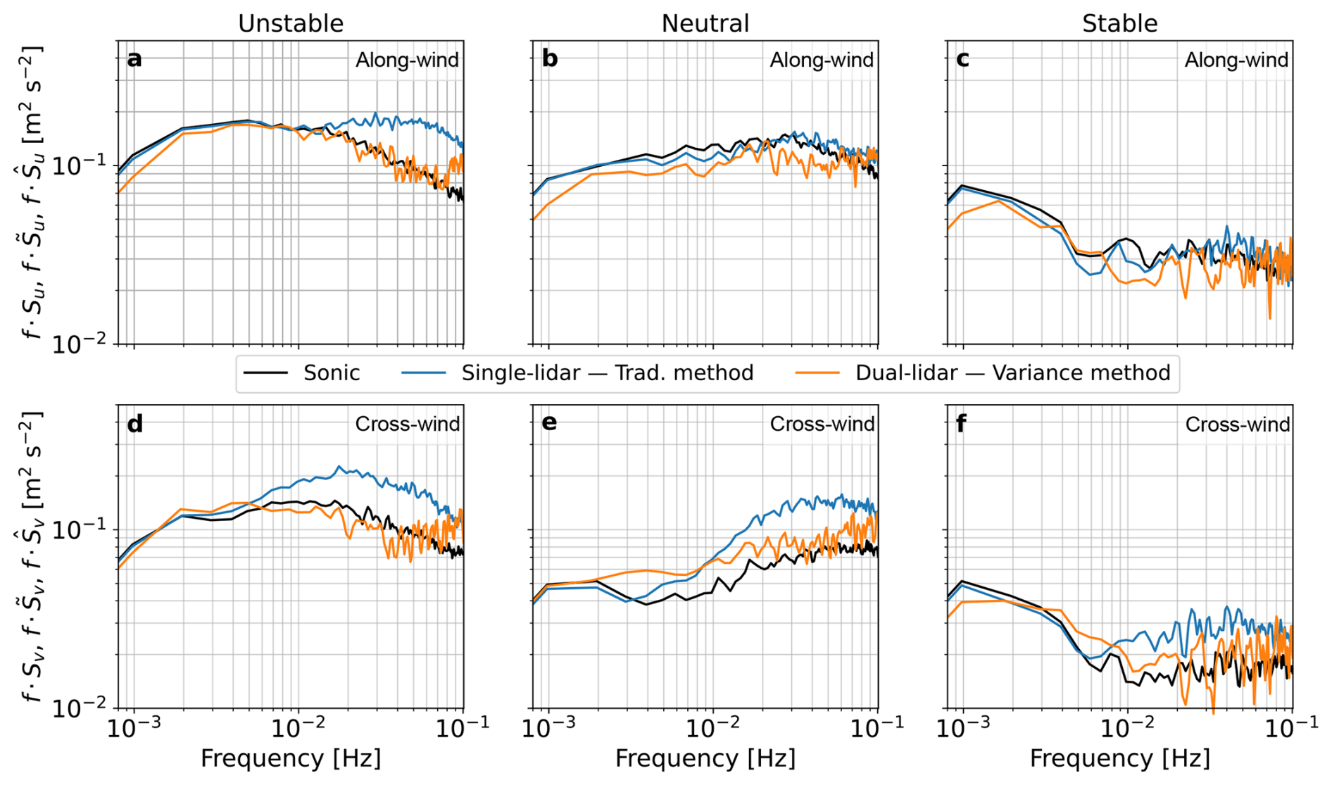
Figure 5 Premultiplied ensemble-averaged spectra of the along-wind and cross-wind velocity components (mean of 30 min premultiplied spectra in each stability class) derived from the traditional and variance methods and compared with sonic anemometer reference spectra.

For the traditional method, the agreement with the reference spectra depends on the velocity component and atmospheric stability. For the along-wind component, good agreement is observed at low frequencies across all stability classes, while under unstable conditions, the spectra exceed the reference at intermediate and high frequencies. For the cross-wind component, the traditional method exhibits higher spectral energy than the reference spectra across all stability regimes, particularly at intermediate and high frequencies.

3.2 Turbulence intensity

Figure 6a–c present scatter plots of the along- and cross-wind TI estimates ${\stackrel{\mathrm{̃}}{\mathrm{TI}}}_u$ and ${\stackrel{\mathrm{̃}}{\mathrm{TI}}}_v$, obtained using the traditional method and plotted against the reference TI values. In contrast, Fig. 6b–d display scatter plots of the along- and cross-wind TI estimates ${\widehat{\mathrm{TI}}}_u$ and ${\widehat{\mathrm{TI}}}_v$, derived using the variance method also plotted against the reference TI. Linear regression models fitted to each dataset are constrained to pass through the origin (zero intercept). The slopes of these regression lines reveal that the traditional method systematically overestimates TI, with ${\stackrel{\mathrm{̃}}{\mathrm{TI}}}_u$ and ${\stackrel{\mathrm{̃}}{\mathrm{TI}}}_v$ being approximately 107 % and 118 % of the reference values, respectively. Conversely, the variance method underestimates TI, yielding ${\widehat{\mathrm{TI}}}_u$ and ${\widehat{\mathrm{TI}}}_v$ values that correspond to approximately 95 % and 97 % of the reference TI. In terms of coefficient of determination (R²), the variance method demonstrates improved performance for the along-wind component, achieving R²= 0.94, compared to R²= 0.89 for the traditional method. However, for the cross-wind component, the traditional method performs better than the variance method, with R²= 0.94 versus R²= 0.90.

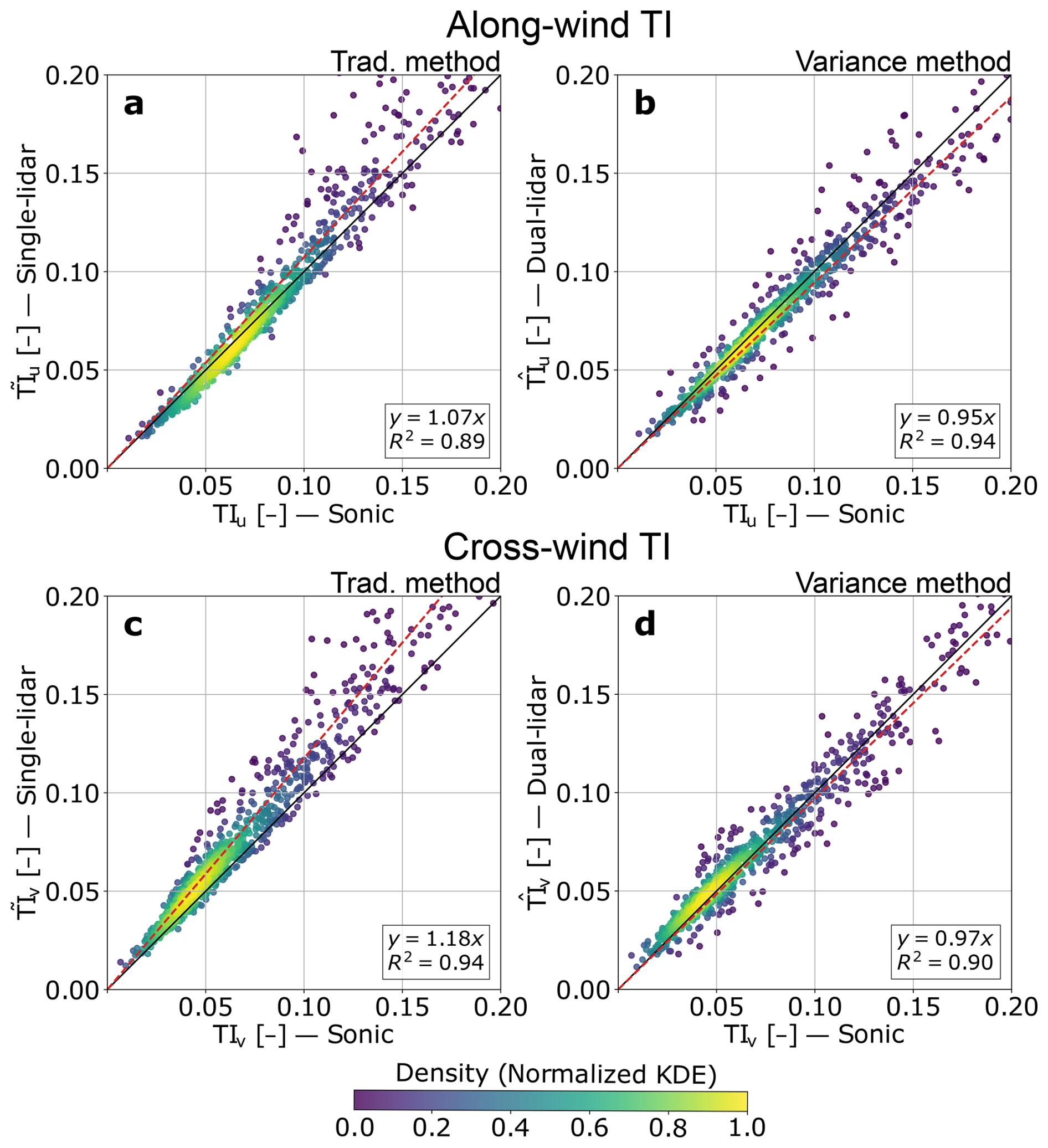
Figure 6 Scatter plots of along- and cross-wind TI estimates obtained using two different methods. Panels (a) and (c) show ${\stackrel{\mathrm{̃}}{\mathrm{TI}}}_u$ and ${\stackrel{\mathrm{̃}}{\mathrm{TI}}}_v$, respectively, derived using the traditional method applied to single-lidar measurements. Panels (b) and (d) show ${\widehat{\mathrm{TI}}}_u$ and ${\widehat{\mathrm{TI}}}_v$, respectively, derived using the variance method based on dual-lidar measurements. Dashed red lines indicate linear regression fits, with the corresponding regression equations and R² values displayed in the bottom-right corner of each panel. Points are color-coded according to normalized kernel density estimation (KDE).

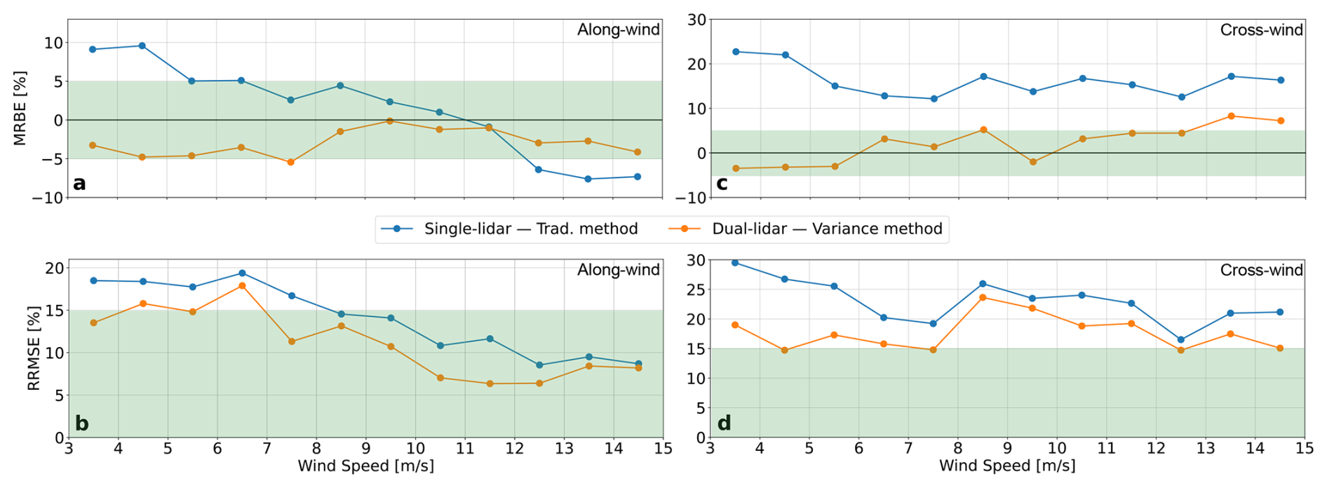
Figure 7 Binned-averaged MRBE (a, c) and RRMSE (b, d) of the along-wind and cross-wind TI derived from the traditional and variance methods as a function of binned-averaged wind speed. The shaded green areas indicate the DNV load-validation acceptance criteria: MRBE within ±5 % and RRMSE ≤15 %. Only bins with sufficient data are shown.

Figure 7 shows the binned-averaged MRBE and RRMSE of the along-wind and cross-wind TI as a function of binned-averaged wind speed. A key observation is that the error metrics associated with the reconstruction of TI using the variance method are consistently lower than those obtained with the traditional method across nearly all wind-speed bins. No strong dependence of MRBE or RRMSE on wind speed is observed, except for the RRMSE of the along-wind TI (Fig. 7b), which clearly decreases with increasing wind speed. The MRBE for the along-wind TI derived using the variance method remains within −5 % to 0 %, while the traditional method yields a considerably wider range of −10 % to 10 %. For both methods, the error metrics associated with cross-wind TI is approximately 1.5 to 1.8 times higher than that of the along-wind TI.

With respect to DNV load-validation acceptance criteria, the variance method provides TI estimates that satisfy the criteria for both MRBE and RRMSE for the along-wind TI, and for MRBE for the cross-wind TI. However, the acceptance criterion for RRMSE of the cross-wind TI is not met with this method. For the traditional method, the DNV acceptance criteria for both MRBE and RRMSE of the along-wind TI are met only at wind speeds above approximately 7 m s⁻¹, while the criteria are not satisfied for the cross-wind TI across the investigated wind-speed range.

Table 2 Comparison of mean MRBE and RRMSE for along-wind and cross-wind TI estimates reconstructed using the traditional method (TM) with single-lidar (SL) measurements and the variance method (VM) with dual-lidar (DL) measurements, across different atmospheric stability conditions. The category “All” represents the full dataset without separation by stability class.

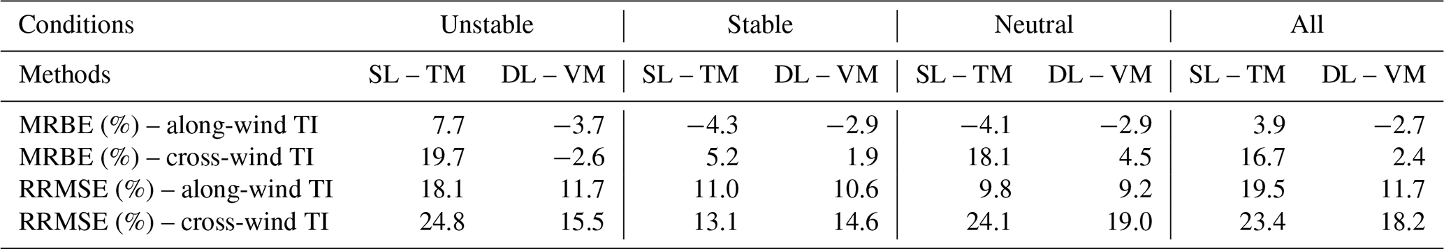
Figure 8 presents the MRBE and RRMSE for along- and cross-wind TI obtained with the traditional single-lidar method and the dual-lidar variance method. The corresponding values are reported in Table 2.

Figure 8 Mean MRBE (a) and RRMSE (b) for along-wind (solid colored bars) and cross-wind (patterned colored bars) TI estimates reconstructed using the traditional method and the variance method across different atmospheric stability conditions. The “All” category represents the entire dataset without differentiation by stability class.

For along-wind TI, the variance method yields negative MRBE for all stability regimes, with values confined to a narrow interval between about −3.7 % and −2.7 %. In contrast, the traditional method spans a wider range, from −4.3 % in stable conditions to 7.7 % in unstable conditions, and remains positive over the full dataset (3.9 %). The spread across stability regimes is therefore larger for the traditional method, whereas the variance method remains nearly constant.

For cross-wind TI, the traditional method produces positive MRBE for all stability regimes, reaching values close to 20 % in unstable and neutral conditions, and 16.7 % over the full dataset. The variance method yields smaller magnitudes, with MRBE between −2.6 % and 4.5 % (depending on stability) and 2.4 % over the full dataset. The range of MRBE across stability regimes is thus substantially reduced compared with the traditional method.

The RRMSE exhibits a similar pattern. For along-wind TI, both methods produce nearly identical errors under stable and neutral conditions (approximately 9 %–11 %). The primary difference arises in unstable conditions, where the variance method reduces the RRMSE from 18.1 % to 11.7 %, representing a substantial improvement. This reduction in unstable regimes largely explains the lower overall RRMSE of the variance method (11.7 %) compared with the traditional method (19.5 %). For cross-wind TI, the variance method also yields lower errors in unstable and neutral conditions, whereas both approaches perform comparably under stable stratification.

4 Discussion

The capability of the variance method applied in a dual-lidar configuration to quantify turbulence was evaluated against the conventional approach commonly used in the wind power industry. Overall, relative to the reference instrument, an underestimation of turbulent energy was observed, as evidenced by both TI and the velocity spectra. This discrepancy is most likely attributable to probe-time averaging inherent to pulsed Doppler lidar measurements, which is governed primarily by the accumulation time Δt and the effective probe length. Both effects introduce temporal and spatial averaging of the wind field, thereby filtering out turbulent fluctuations with scales smaller than the probe volume. To preserve smaller turbulent structures, the accumulation time must be reduced. Thiébaut et al. (2025) demonstrated that decreasing the accumulation time at each LOS position from 0.8 s – corresponding to a sampling rate of 0.25 Hz in standard commercial lidar configurations – to 0.2 s, corresponding to a 1 Hz sampling rate for the WindCube v2.1, increases the along-wind variance obtained from the variance method by approximately 7 %, without significantly reducing data availability (a decrease of 0.5 %).

Building on the well-known impact of probe-volume averaging, Manami et al. (2025) proposed a method to recover part of the filtered turbulent energy by exploiting Doppler spectral information rather than relying solely on LOS velocities. Their results indicate that a larger fraction of the turbulence statistics can be retrieved when spectral broadening effects are taken into account. In this context, the systematic underestimation of turbulent energy observed in the present study can be interpreted as a direct consequence of conventional velocity-based retrieval techniques, which remain intrinsically affected by probe-volume averaging. The comparison therefore highlights both the fundamental limitations imposed by probe length and accumulation time, and the potential of advanced spectral-based approaches for improving turbulence characterization with pulsed Doppler lidars.

The variance method yields lower mean MRBE and RRMSE across all stability regimes except for the cross-wind TI under stable conditions. Under stable stratification, TI is generally low and often dominated by small-scale fluctuations, which limits the overall turbulent energy available. In such cases, the reduced energy content can diminish the magnitude of inter-beam effects in the traditional reconstruction, leading to smaller errors. Under neutral and unstable conditions, turbulence is typically stronger and characterized by a broader range of energetic scales, which increases the sensitivity of inter-beam reconstruction methods to spatial separation between beams. While intermittent turbulence and violations of homogeneity can also occur under stable conditions – particularly in the presence of strong shear – the higher overall turbulence levels commonly observed under neutral and unstable stratification tend to amplify inter-beam effects in the traditional method. Because the variance method relies directly on LOS velocity statistics and avoids inter-beam reconstruction, it provides more reliable estimates of TI under these conditions, despite remaining sensitive to intra-beam averaging.

The corresponding spectral differences reflect the distinct sampling and reconstruction mechanisms of the two approaches. At low frequencies, the traditional method captures large-scale, slowly evolving motions that remain coherent over the scan volume, leading to good agreement with the reference sonic measurements. In contrast, spectra derived from the variance method show a systematic underestimation of energy in the low-frequency range. This behavior does not arise from direct spatial filtering by the finite probe length, which primarily affects small-scale fluctuations, but from the nature of the variance method itself. Large-scale turbulent motions are nearly uniform across the lidar probe volume and therefore mainly affect the mean LOS velocity, while producing little variability in the probe. Because the variance method relies on velocity fluctuations in the sampling volume rather than on the absolute velocity, these coherent motions contribute less energy to the reconstructed spectrum than they do in point measurements from the sonic anemometer.

At intermediate frequencies, where turbulent fluctuations become increasingly decorrelated across the probe volume, spectra derived from the variance method show good agreement with those obtained from the sonic anemometer. At higher frequencies, however, spectra from the variance method depart from the sonic reference and exhibit a white-noise behavior, reflecting the growing influence of instrumental noise and the limited sensitivity of the method at small scales. At high frequencies, the traditional method modifies the reconstructed spectrum through a wavenumber-dependent response associated with beam separation, as a consequence of the inter-beam effect, which can artificially enhance small-scale energy (Kelberlau and Mann, 2020). This effect is strongest under neutral and unstable conditions, where the inertial subrange is well developed, and is reduced under stable conditions, where high-wavenumber turbulence is suppressed.

The magnitude of inter-beam effects further depends on local site characteristics. These effects arise when different beams probe flow regions that are not dynamically coherent, for example, due to mean-flow acceleration over terrain features, sheltering effects, or localized shear and recirculation induced by surface roughness or obstacles. When such spatial gradients are present, sequential sampling of different flow regions combined with advection can map stationary spatial variability onto temporal fluctuations, introducing apparent variance when the beams are combined. This spurious variability does not reflect true turbulence but rather space–time sampling effects, and it can either amplify or attenuate the apparent turbulent energy. As a result, the performance of the traditional method can be strongly site dependent, whereas the variance method is less sensitive to such effects. At the present offshore site, the flow is expected to be relatively homogeneous and free of strong spatial gradients; therefore, the differences between the variance and traditional methods reported here likely represent a lower bound, and larger discrepancies may occur at more complex sites.

In contrast, the variance method is impacted primarily by the intra-beam effect, which is systematic and thus more predictable. This makes the variance method potentially more robust and transferable across different sites. Furthermore, TI derived from the variance method exhibited smaller variations across the stability regimes examined, suggesting that atmospheric stratification has a weaker influence on its ability to capture the underlying turbulence level compared to the traditional method.

For both methods, a marked difference was observed between the along-wind and cross-wind TI, with significantly larger errors associated with the latter. Nevertheless, the variance method consistently yielded lower errors than the traditional approach. Velocity reconstruction relies on LOS measurements acquired at different times, and the associated temporal decorrelation affects the velocity components differently. Along-wind fluctuations, which are advected by the mean flow, remain correlated over the scan cycle, whereas cross-wind fluctuations decorrelate more rapidly (Sathe and Mann, 2012). As a result, combining temporally separated LOS measurements can lead to a reduced or distorted estimate of cross-wind turbulent energy. The variance method mitigates this limitation by avoiding inter-beam reconstruction, although the underlying decorrelation remains intrinsic to sequential scanning. A fully simultaneous multi-beam lidar configuration, analogous to an ADCP, would remove this source of decorrelation and is therefore expected to improve cross-wind turbulence estimates. However, achieving true simultaneity would require multiple independent transmit–receive channels operating at different beam angles, rather than a single laser sequentially steered by a scanner. This would substantially increase optical, electronic, and calibration complexity, and consequently the overall system cost.

5 Conclusions

The variance method applied in a dual-lidar configuration demonstrates improved performance compared to the traditional method for MRBE and RRMSE for both along- and cross-wind TI. Because it is primarily affected by the intra-beam effect, which is systematic and physically interpretable, the variance method is largely site independent and broadly applicable, thereby overcoming the main limitation of the traditional method associated with unpredictable inter-beam errors. Moreover, turbulence estimates derived from the variance method remain consistent across varying atmospheric stability conditions, highlighting its resilience to stratification effects. Taken together, these features indicate that the dual-lidar approach is now sufficiently mature for validation and practical deployment in ground-based wind measurements, albeit at the expense of increased instrumentation costs associated with the use of two lidar systems.

Cross-wind turbulence exhibits higher uncertainty than along-wind turbulence due to temporal decorrelation associated with sequential LOS sampling. While the variance method reduces the resulting errors compared with the traditional approach, this limitation remains intrinsic to scanning Doppler lidars. Along-wind turbulence is less affected by this decorrelation, as its dominant fluctuations tend to remain coherent over the scan cycle, which is consistent with the lower uncertainties observed in the along-wind component.

Further improvements in lidar technology and scanning strategies can enhance the performance of the variance method. With current profilers, performance is influenced by the accumulation time and probe length, which must be balanced to maintain adequate data availability while preserving sensitivity to turbulent fluctuations. Temporal decorrelation associated with sequential scanning remains an inherent limitation of current systems and particularly affects cross-wind turbulence estimates. Addressing this limitation through future instrument developments could further improve turbulence retrievals. Nevertheless, the variance method remains a robust and versatile approach for accurate site-independent turbulence measurements, supporting reliable wind energy assessments and load modeling.