How well can the Mann model describe typhoon turbulence?

More and more wind farms are planned and built in regions prone to tropical cyclones. However, the current International Electrotechnical Commission (IEC) standard provides no clear guidelines on how to account for turbulence occurring during tropical cyclones. This study investigates how well the Mann uniform shear model, a model referenced by the IEC, can model turbulence during tropical cyclone conditions. We analyzed sonic anemometer measurements at 60 m from four typhoon cases in the South China Sea. The Mann model was fit to the one-point spectra in different locations in the typhoon structure. We found that the Mann model can fit the observed spectra outside the typhoon eye and the rainbands to a certain extent. However, several deficiencies are identified. (1) In the outer-cyclone region, spectral energy at wavenumbers smaller than $\mathrm{3}\times {\mathrm{10}}^{-\mathrm{3}}$ m⁻¹ is generally larger than predicted by the Mann model, likely reflecting the presence of mesoscale wind fluctuations. (2) Consistent with previous studies, excess spectral energy is observed at wavenumbers larger than 10⁻¹ m⁻¹ in the inner-cyclone and eyewall regions of one typhoon; however, it cannot be ruled out that this excess energy may be related to measurement quality. (3) In the inner-cyclone region, the peak wavenumbers of the alongwind and crosswind spectra are often closer together than predicted by the Mann model. In these cases, the crosswind component exhibits larger-than-predicted spectral energy within the energy-containing subrange. This study can serve as a baseline for further research addressing turbulence in tropical cyclones in the context of structural engineering.

1 Introduction

In recent years, more and more wind farm projects have been planned and deployed in regions affected by tropical cyclones. These storms are associated with extreme wind speeds, which can pose serious risks to civil structures, including wind turbines. For example, typhoons Yagi (2024), Maria (2018), Rammasun (2014), and Usagi (2013) caused severe structural damage to wind turbines (Zhou et al., 2025; Li et al., 2022; Chen and Xu, 2016). This highlights the need to assess whether the International Electrotechnical Commission (IEC) standard for wind turbines (IEC, 2019) is adequate for specifying wind conditions for tropical cyclone conditions as well. For these conditions, one of the turbine design parameters, V_ref – the 10 min mean value of the 50-year wind speed at hub height – has garnered some attention both in the IEC standard and from researchers (e.g., Ott, 2006; Larsén and Ott, 2022; Imberger et al., 2024). Recently, there have also been a few studies highlighting the importance of wind shear and veer during tropical cyclones in wind turbine load assessment (e.g., Sanchez Gomez et al., 2023; Müller et al., 2024). There have been studies investigating turbulence characteristics during tropical cyclone conditions; however, studies of their impact on wind turbine loads are sparse.

Cao et al. (2009) observed turbulence characteristics during Typhoon Maemi (2023) to be comparable to non-typhoon conditions. In particular, they found that the wind speed power spectrum could be expressed well with the von Kármán spectrum (von Kármán, 1948). However, some studies report that turbulence spectra measured under tropical cyclone conditions deviate from standard spectral models frequently used in wind engineering. From turbulence measurements during the Coupled Boundary Layer Air–Sea Transfer (CBLAST) Hurricane experiment, Zhang et al. (2011) calculated turbulence spectra in the outer-cyclone region, away from the rainbands. The spectra had forms similar to those of the Kaimal model (Kaimal et al., 1972); however, energy was shifted to higher frequencies. This agrees with measurement-based findings from Li et al. (2012) and with the large-eddy simulation (LES) modeling work by Worsnop et al. (2017). Li et al. (2015) further found excessive energy in the inertial dissipation range. They argued that this enhanced energy at high frequencies was likely related to sea spray. However, it could not be ruled out that it could also be caused by measurement artifacts such as tower wake effects, tower vibrations, or sensor noise (Barthlott and Fiedler, 2003; Gao et al., 2024; Kaimal and Finnigan, 1994).

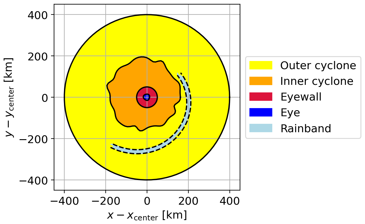
Tropical cyclone turbulence is strongly non-stationary (e.g., Huang et al., 2020). This has prompted the development of various analysis methods within the bridge and structural engineering communities. Examples include evolutionary spectra (Priestley, 1965) and empirical mode decomposition (e.g., Xu and Chen, 2004; Wang et al., 2018; Tao and Wang, 2019). The non-stationary nature of tropical cyclone turbulence is linked to the large-scale, organized structure of these storms. The wind field varies across different regions of a tropical cyclone, including the eye, eyewall, and rainbands. These key regions of tropical cyclones are illustrated in Fig. 1. Wind speeds are the highest in the eyewall, where the vertical wind component is also significant. As a tropical cyclone passes over a wind farm, turbines experience different regions over time, causing wind characteristics to change both within and between these regions.

Figure 1 Illustration of typhoon regions, as defined for the analysis.

Within different regions of the tropical cyclone, embedded mesoscale flow structures can further affect tropical cyclone turbulence. Li et al. (2015) discussed the role of boundary layer rolls, horizontal elongated counter-rotating vortex structures, in tropical cyclone turbulence. Boundary layer rolls have been observed in various tropical cyclones (Zhang et al., 2008; Huang et al., 2018; Tang et al., 2021). Foster (2005) and later Gao and Ginis (2014) showed how boundary layer rolls form in idealized tropical cyclone simulations. Such roll structures affect turbulent fluxes in the tropical cyclone boundary layer (Zhu et al., 2010; Tang et al., 2021), which can cause the turbulence behaviors to deviate from classical turbulence modeling. Worsnop et al. (2017) noted that enhanced coherence apparent in their LES could be related to these roll structures. In areas most interesting for wind energy, close to the coast, turbulence can be further complicated by the land and internal boundary layers (He et al., 2022).

For both turbine design and operation, it is crucial to know how a tropical cyclone affects the loads on turbines. Worsnop et al. (2017) analyzed turbulence based on LES and concluded that adjustments to wind turbine standards may be needed to capture the characteristics of turbulence in tropical cyclones. To simulate wind turbine loads, the turbulence wind field needs to be modeled in a three-dimensional space around the turbine (Dimitrov et al., 2017). The IEC standard recommends using a modified version of the Kaimal model (Kaimal et al., 1972) or the Mann uniform shear model (Mann, 1994) (hereafter referred to as the Mann model). The Mann model is based on rapid distortion theory (RDT), assuming that turbulence eddies are elongated under linear wind shear over their lifetime. The Mann model is well established in wind energy but has been only sparsely evaluated for tropical cyclone conditions. Han et al. (2014) compared it to two tropical cyclone spectra averaged over entire typhoon passages. They find reasonable agreement but a slight underestimation of the spectral peak. Larsen et al. (2016) present a fit of the Mann model to the measurements from the outer-cyclone region published in Zhang et al. (2011), which also suggests reasonable agreement. However, comprehensive evaluations of the Mann model across different regions of tropical cyclones are lacking, and the suitability of the RDT as a basis for such conditions remains uncertain. Moreover, the model is formulated for microscale turbulence and does not account for wind fluctuations acting on larger scales.

Wind speed power spectra often exhibit a spectral gap that distinguishes three-dimensional, microscale turbulence from two-dimensional, larger-scale fluctuations. The latter has been referred to by different terms in the literature. In this study, the term “mesoscale fluctuations” is used. Turbulence models such as the Mann model are designed to describe only the microscale range. However, particularly over the ocean, the spectral gap is not always distinct, and mesoscale fluctuations can contribute significantly to the spectral energy density at timescales longer than a few minutes. Consequently, spectral energy at these scales can exceed that predicted by the Mann model, as demonstrated by De Maré and Mann (2014). To represent both mesoscale and microscale wind variability, Larsén et al. (2016) proposed a model based on measurements from two stations (from the surface to 100 m), which was later confirmed by measurements up to 245 m from another station (Larsén et al., 2021). Several subsequent studies have further investigated this topic worldwide. For example, Cheynet et al. (2018) used FINO 1 data to conduct a detailed spectral analysis under different stability conditions. Syed and Mann (2024) built on this work by extending the Mann model toward lower wavenumbers through the inclusion of manually added mesoscale fluctuations. Mesoscale fluctuations have been shown to be enhanced in the presence of organized atmospheric structures such as open cells and fronts (Larsén et al., 2019). These findings suggest that mesoscale fluctuations may play an important role in tropical cyclones and could be linked to the observed non-stationarity.

Overall, the Mann model may face substantial limitations when applied to tropical cyclone conditions. How well the Mann model can fit tropical cyclone turbulence has not yet been systematically addressed. In particular, it is not clear how well the Mann model can describe the turbulence behavior in different tropical cyclone regions, and how large the contribution of mesoscale fluctuations is during tropical cyclone conditions. In this study, we investigate tropical cyclone turbulence in different cyclone regions by analyzing high-frequency measurements of four typhoons in the South China Sea. In particular, we assess where the Mann model can fit tropical cyclone turbulence and where it may have limitations.

In the following, the measurements used for the analysis are introduced in Sect. 2, where the methods for data processing and for calculating the power spectra are introduced. The Mann model and the fitting are also explained in this section. Results are presented in Sect. 3, followed by discussions and conclusions in Sects. 4 and 5.

2 Data and methods

2.1 Data

We use measurement data from four typhoons to study turbulence spectral behaviors. These are Typhoon Hagupit in 2008, Typhoon Nuri in 2008, Typhoon Prapiroon in 2006, and Typhoon Chanchu in 2006. Table 1 summarizes the mast locations, the height of the analyzed data, the instruments, and the sampling frequencies of all measurements. The locations of the masts are also shown in Fig. 2, with Fig. 2b–e being a close-up view of the four locations and their surroundings. We use the flux footprint estimate described in Smedman et al. (1999) (their Appendix A) to roughly identify land-dominated fetches. According to this estimate, over 60 % of the total flux footprint at a measurement height of 60 m is contained within a 6 km upwind distance. The corresponding land-dominated fetch areas are shaded red in Fig. 2b–e. To make the best use of the limited measurement data, we analyze measurement periods with wind direction from both land-dominated and water-dominated sectors. The fetch effect is addressed in the analysis.

Table 1 Summary of the measurement data during four tropical cyclones.

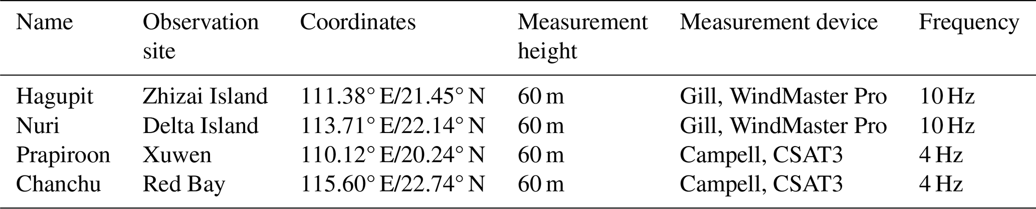
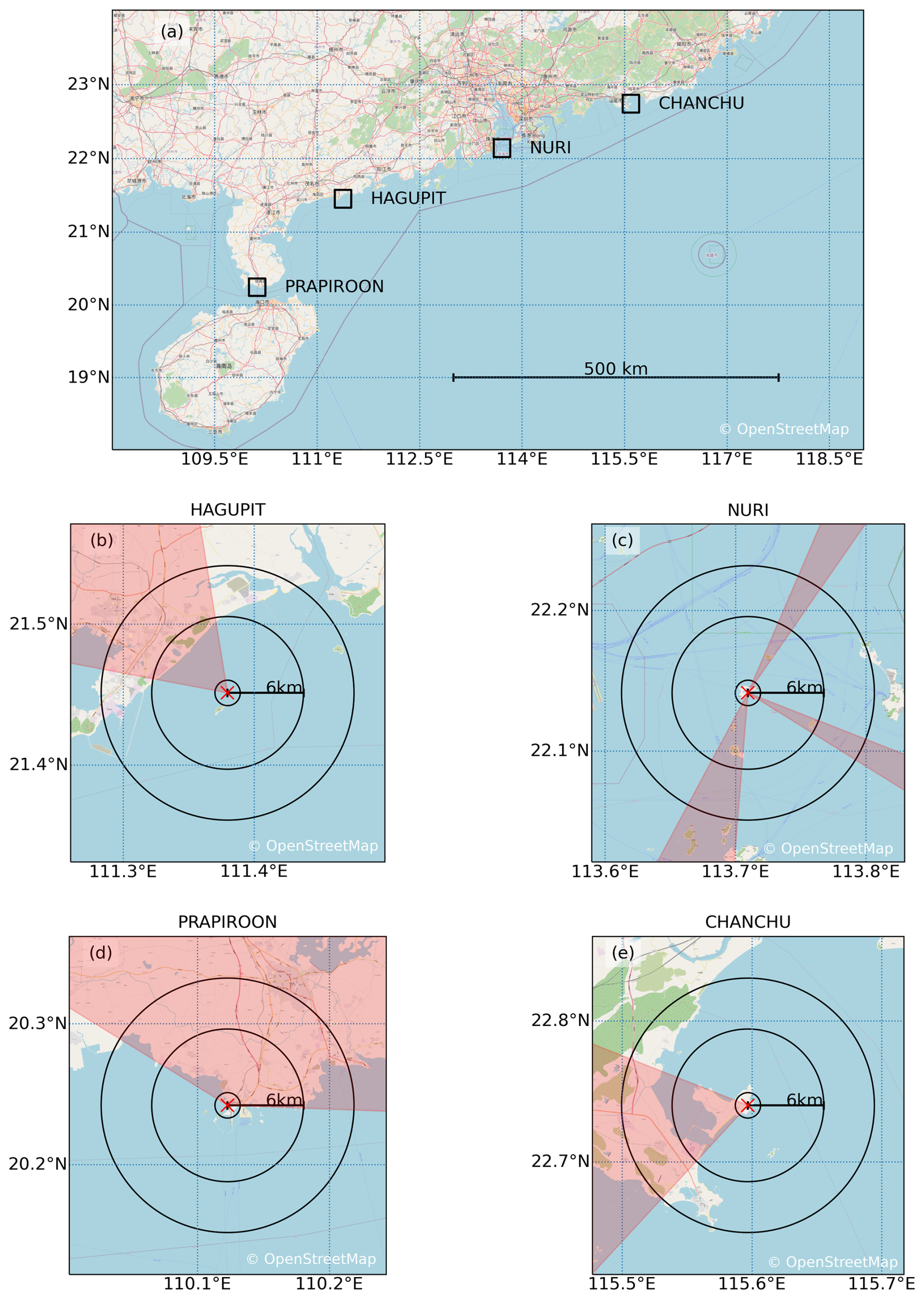
Figure 2 Measurement locations during four tropical cyclones. Panel (a) gives a large-scale overview, and panels (b)–(e) feature the detailed environment given by the black rectangles in panel (a). The red cross in panels (b)–(e) indicates the station location. The black circles give distances of 1, 6, and 10 km. The red shading indicates wind directions, where the innermost 6 km is influenced by land (adapted from OpenStreetMap).

The measurements of Typhoon Hagupit are described in detail in Li et al. (2012); they were also analyzed in other studies (Liu et al., 2011; Li et al., 2015; Wenchao et al., 2011). The three-dimensional wind speed was measured using a Gill WindMaster Pro ultrasonic anemometer at 10 Hz. The device is mounted at 60 m on the Bohe meteorological tower located on Zhizai Island in Guangdong Province (Fig. 2b). The island is approximately 120 m in length and 50 m in width, with a distance of about 4.5 km to the southwest of mainland China. The tower base is 11 m above sea level. To the west and southwest, the wind is fairly exposed to open waters. To the northwest, mainland China affects the wind at the measurement height.

The measurements used to analyze Typhoon Nuri are described in Li et al. (2015). The three-dimensional wind field was measured by a Gill WindMaster Pro ultrasonic anemometer at 60 m at a 10 Hz frequency. The measurement mast stands on Delta Island, at the entrance of the Pearl River estuary (Fig. 2c). The tower base is 93 m above sea level. The wind is fairly exposed to open waters. Smaller islands are within a 6 km distance from Delta Island. Sectors from affected directions are labeled “mixed fetch” in the following analysis. The city of Macau is more than 10 km to the northeast of the measurement tower.

The wind field used for the analysis of Typhoon Prapiroon was measured at 4 Hz by a CSAT3 ultrasonic anemometer from Campell. The ultrasonic anemometer is installed at 60 m on a meteorological tower in Xuwen, in the southwest of Guangdong Province (Fig. 2d). The tower is located in the coastal region facing the Qiongzhou Strait to the south. The distance to the sea is around 200 m to the west and 700 m to the south and southeast. In these directions, the tower is exposed to winds from the sea. In the northern sectors, the wind comes from the land mass.

Typhoon Chanchu's wind field was measured by a CSAT3 ultrasonic anemometer from Campell at 4 Hz. The anemometer is installed at 60 m on a meteorological tower on the Red Bay peninsula in Shanwei, northern Guangdong Province (Fig. 2e). The Red Bay peninsula faces the South China Sea to the southeast. The distance to the shore is around 500 m to the south and east and 1.5 km to the north. To the west, the wind comes from the land, while to the other wind directions, the wind comes from the water.

2.1.1 Data preprocessing

The quality of the measured time series was carefully examined. Special care was taken for two reasons. First, tropical cyclones are associated with strong wind speeds, large waves, and intense rainfall. These severe conditions can cause technical difficulties that affect the quality of the data. One consequence is frequent spikes in wind measurements. Second, since tropical cyclone measurements only include a few hours, the data are especially valuable. Therefore, efforts are made to retain as much data as possible. The data were processed through five steps:

1. Correction of w-boost bug. Gill WindMaster Pro anemometers produced between 2006 and 2015 are known to be affected by a firmware bug, known as the w-boost bug (Billesbach et al., 2018). The bug can be corrected by multiplying positive (upward) vertical wind components by 1.166 and negative (downward) values by 1.289. The measurements of typhoons Nuri and Hagupit are most likely subject to the w-boost bug, and the correction has been applied to these datasets.

2. Filtering of spikes. Spikes are detected in two steps. First, a fixed threshold is applied: horizontal wind speeds exceeding 65 m s⁻¹ are flagged, corresponding to the measurement limit of the CSAT3 anemometers. Second, remaining spikes are identified using a moving median filter. Details of the moving median filter are provided in Appendix A.

3. Filtering of repeating values. For Typhoon Chanchu, the measurements of the three wind components feature episodes with consecutive repeated values. An example is shown in Appendix A (Fig. A1b). We checked the data for episodes where one of the three components does not change for longer than 10 s and removed intervals with more than 5 % of these repeated values.

4. Filtering of flickering. In the measurements of the four typhoons, there are episodes where individual wind-component measurements alternated between large and small values. An example is shown in Appendix A (Fig. A1c). To detect these episodes, the difference between consecutive measurement values is calculated. The data are removed when more than 5 % of these differences are larger than 5 m s⁻¹ within a 5 min data segment.

5. Filling the data gaps. Continuous data series are needed to calculate time spectra. Therefore, gaps in the data are filled. Gaps from removed spikes are linearly interpolated. If the percentage of spikes, repeated values, or values removed due to flickering is more than 5 % in any of the wind components in a 5 min segment, the segment is disregarded. To make the best use of the data, disregarded data are filled using data from a time window of 15 min before to 15 min after the center of the disregarded data. Only segments with less than 15 % filled data are used to calculate spectra.

2.1.2 Power spectra calculation

Wind speed power spectra are calculated similarly to Welch's method (Welch, 1967) for 30 min segments with 50 % overlap. Details are provided in the following. In each 30 min segment, the wind field is decomposed along the mean horizontal wind vector into the alongwind component u, the crosswind component v, and the vertical wind component w. For each 30 min segment, the two-sided power spectrum in the frequency domain is calculated using fast Fourier transform, and no Hamming window is applied. The Taylor hypothesis is used to transform the spectra from the frequency domain to the wavenumber domain through

$$\begin{array}{}\text{(1)}& k=\mathrm{2}\mathit{\pi }\cdot f/U,\end{array}$$

where k is the wavenumber, f the frequency, and U the average wind speed over the 30 min segment. Spectra are smoothed by averaging the values of the normalized spectral power in bins of log ₁₀(k), with 10 bins per decade in k. The median spectrum is then calculated by taking the median of the normalized spectral power across the different spectra for each k bin.

Wind conditions during tropical cyclones are often non-stationary, and both the wind direction and the mean wind speed can vary substantially within a 30 min segment. However, in contrast to non-stationary methods used to analyze microscale turbulence in tropical cyclones (e.g., Xu and Chen, 2004; Tao and Wang, 2019), our study aims to include the impact of non-stationarity on the wind speed power spectra. For this reason, we do not apply any filtering based on changes in the mean wind speed or the variance. We acknowledge that this introduces uncertainties in the definition of U for each segment, which may in turn affect the transformed wavenumber spectra, particularly the estimated energy density at the corresponding wavenumbers. Moreover, a meaningful decomposition into the u and v wind components is only possible when the wind direction does not change significantly. Therefore, we retain only the 30 min segments in which the maximum change in wind direction is less than 20°, based on 10 min moving averages. Additionally, to reduce the influence of non-stationarity, the time series of u, v, and w are linearly detrended prior to computing the spectra.

2.2 The Mann model and the fitting

The Mann model applies RDT on a von Kármán isotropic tensor (von Kármán, 1948). Here the main assumptions include constant vertical shear and neutral atmospheric stability. RDT allows for the assessment of how the wind shear acts on a wind field represented as a superposition of Fourier modes. Intuitively, the effect of wind shear can be understood by considering its effect on individual turbulent eddies. The shear elongates the eddies in the mean shear direction. Mann (1994) extended RDT by assuming a characteristic non-dimensional lifetime (Γ) of turbulent eddies as a function of wavenumber. Γ controls the total stretching of the eddies in a steady state. To illustrate how Γ affects the spectra, Fig. 3 shows normalized u, v, and w spectra (kF_u, kF_v, kF_w) and uw cospectra (kF_uw) for different Γ values. For a Γ value of zero, the turbulence is isotropic. With increasing Γ, the energy in the kF_u and, to a lesser extent, in kF_v and kF_uw increases, and the energy in kF_w decreases. At the same time, the peak wavenumber k_p changes. It becomes smaller for the u and v components and larger for the w component. Note that the spectral energy increases more for the u component than for the v component. Also, the difference between k_p for the u and v components increases. A key advantage of the Mann model is that it incorporates the second-order structure of homogeneous turbulence in a neutral atmosphere using only three parameters.

Figure 3 Spectra obtained by the Mann turbulence model with different Γ values. Here L is 30 m, and $\mathit{\alpha }{\mathit{ϵ}}^{\mathrm{2}/\mathrm{3}}$ is 1 m${}^{\mathrm{4}/\mathrm{3}}$ s⁻².

Apart from Γ, the other two adjustable parameters of the Mann model are (1) a turbulent length scale (L) and (2) a parameter controlling the decay of turbulence, $\mathit{\alpha }{\mathit{ϵ}}^{\mathrm{2}/\mathrm{3}}$. L is the size of the largest energy-containing eddies, and it controls k_p. In $\mathit{\alpha }{\mathit{ϵ}}^{\mathrm{2}/\mathrm{3}}$, α is Kolmogorov's constant, and ϵ is the turbulent dissipation rate. $\mathit{\alpha }{\mathit{ϵ}}^{\mathrm{2}/\mathrm{3}}$ modulates the magnitude of the spectra and is related to the standard deviation of the wind components (Mann, 1994).

We estimate the three Mann model parameters by finding the fit of the Mann model to the spectra obtained from measurements that have a minimal difference between the normalized autospectra of the three velocity components and the normalized uw cospectra. Similar to Syed and Mann (2024), we use a downhill simplex algorithm (McKinnon, 1998) to minimize the error function (F_error):

$$\begin{array}{}\text{(2)}& \begin{array}{rl}{F}_{\mathrm{error}}=& \sum _{i=\mathrm{1}}^{\mathrm{3}}\sum _{j=\mathrm{1}}^N\left|k_j\cdot F_{i,\mathrm{Mann}}\left(k_j\right)-k_j\cdot F_{i,\mathrm{meas}}\left(k_j\right)\right|\\ & +\sum _{j=\mathrm{1}}^N\left|k_j\cdot F_{\mathrm{13},\mathrm{Mann}}\left(k_j\right)-k_j\cdot F_{\mathrm{13},\mathrm{meas}}\left(k_j\right)\right|.\end{array}\end{array}$$

Here, F_i,Mann and F_i,meas (i=1, 2, 3) are the autospectra of the u, v, and w components of the Mann model and the measured spectra, respectively. F₁₃ is the uw cospectrum. N is the number of wavenumbers in the spectra after the logarithmic averaging. In order to get the best model fit in the energy-containing range of the spectra, only k<0.1 m⁻¹ is used for the fit. To avoid extreme, physically unreasonable values of these parameters when fitting the Mann model, we limit the parameter range according to values usually found in the literature under atmospheric conditions: $L\in [\mathrm{0},\mathrm{300}]$ m, $\mathit{\alpha }{\mathit{ϵ}}^{\mathrm{2}/\mathrm{3}}\in [\mathrm{0},\mathrm{2}]$ m${}^{\mathrm{4}/\mathrm{3}}$ s⁻², and $\mathrm{\Gamma }\in [\mathrm{0},\mathrm{5}]$.

2.3 Analysis of turbulence behaviors in various typhoon regions

Wind properties vary greatly between different regions in typhoons, be it the eye, eyewall, rainbands, or outer region. Therefore we define regions with similar wind field characteristics, on which we base the analysis of the turbulence spectra. We distinguish between five regions as illustrated in Fig. 1. These regions are (1) the outer-cyclone region; (2) the inner-cyclone region; (3) the eyewall, defined as a radially narrow band including the strongest horizontal wind speeds; (4) the eye, a region with low to moderate horizontal wind speeds, radially inward of the eyewall; and (5) the rainbands. To distinguish between these regions, we use the mean wind speed from the measurements (WS) (10 min running average at 60 m measurement height), the distance to the cyclone center (R), and the radius of the maximal wind speed (RMW). Both R and RMW are obtained from the International Best Track Archive for Climate Stewardship (IBTrACS) (Gahtan et al., 2024; Knapp et al., 2010) and linearly interpolated to the measurement time. The spectral behaviors are not analyzed for the eye and rainband regions because the wind direction changes significantly in these regions, which makes the decomposition of the wind vector into the u and v wind components ambiguous. The boundaries of the outer-cyclone, inner-cyclone, and eyewall regions are set roughly based on the following criteria:

• The outer-cyclone region includes measurements where R ≲ 400 km and WS ≲ 17 m s⁻¹. We take R = 400 km as the outer boundary of the outer-cyclone region because the distance of the outermost closest isobar is roughly 400 km for the four analyzed typhoons, according to the IBTrACS.

• The inner-cyclone region includes measurements with WS ≳ 17 m s⁻¹ and R ≳ 2 RMW.

• The eyewall includes measurements where R ≲ 2 RMW. Note that eyewall asymmetries cannot be addressed by these criteria. The inner edge of the eyewalls is taken where WS ≃ 25 m⁻¹, based on visual inspection of the measured wind speed time series.

Flexibility in these criteria is allowed such that the time series can be divided into continuous periods belonging to the same region. We further distinguish between the front and the back sectors of the typhoon, i.e., the measurement period before and after the time step where the cyclone center is closest to the measurement station, a similar approach to Li et al. (2012).

For Typhoon Prapiroon, a rainband is identified by using an index of enhanced fluctuations in the vertical wind, as is shown in Sect. 3.1. This approach was proven to be successful when verified by a satellite-based precipitation dataset, which shows consistent coverage of rainbands with regions of large vertical wind fluctuations. Specifically, we use the Integrated Multi-satellite Retrievals for the Global Precipitation Measurement Mission (IMERG) (Huffman et al., 2023). This is a global, gridded precipitation dataset with a resolution of 30 min and 0.1°, available from 1988 to the present. The IMERG data were obtained by the Integrated Multi-Satellite Retrieval for GPM algorithm v7, which inter-calibrates, merges, and interpolates measurements, including satellite microwave precipitation estimates, microwave-calibrated infrared satellites, and precipitation gauge analyses. The dataset has previously been used successfully to characterize tropical cyclone precipitation (Rios Gaona et al., 2018). Note that regions other than the rainband are also affected by precipitation and convection, though to a lesser extent.

3 Results

3.1 Meteorological background of the typhoons

We first give a short overview of the four typhoons to aid in understanding how these typhoons influenced the wind fields and turbulence spectra during different periods and, thereby, different typhoon regions. The measured horizontal wind speed, direction, and vertical wind speed are shown in Figs. 4–7 (subplots in the left panel) alongside the typhoon track (subplot in the right panel) for the four typhoons. Periods analyzed in more detail are marked in blue and labeled for reference, with the label “FO” for front outer cyclone, “FI” for front inner cyclone, “FEW” for front eyewall, “BI” for back inner cyclone, “BO” for back outer cyclone, and “BEW” for back eyewall, both in the left and right panels.

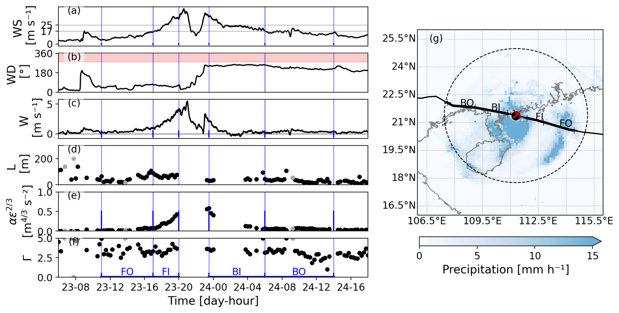
Figure 4 (a–c) Measured wind field at 60 m during Typhoon Hagupit (10 min running average): (a) horizontal wind speed, (b) wind direction (red shading indicates wind directions, where the innermost 6 km is influenced by land), (c) vertical wind speed, (d–f) fitted Mann parameters (cases in which one of the fitted parameters equals the prescribed parameter limits are shown in gray), (g) typhoon track from IBTrACS (solid black line, from west to east), measurement station (red cross), precipitation at 22:00 UTC on 23 September from IMERG (shading), cyclone center at that time (black point), and 400 km distance to cyclone center (dashed black line). Typhoon regions further analyzed are marked in panels (f) and (g): front outer cyclone (FO), front inner cyclone (FI), back inner cyclone (BI), and back outer cyclone (BO).

Typhoon Hagupit's track over the measurement mast is shown in Fig. 4g; also shown are the precipitation data from IMERG at 02:30 UTC on 4 August. Hagupit formed over the northwest Pacific in September 2008; see Fig. 4g. Hagupit moved westwards and entered the South China Sea through the Luzon Strait. Around 00:00 UTC on 24 September, Hagupit made landfall on mainland China at Dianbai, close to the measurement station. The passing of the typhoon is clearly shown in the measured wind field (Fig. 4a–c). At 06:00 UTC on 23 September, the station was around 450 km to the northwest of the cyclone center. The peak in wind speed at around 09:00 UTC on 23 September is most likely associated with a rainband, also present in the IMERG dataset (not shown). After the passing of the rainband, the wind speed increased, while the typhoon approached the measurement location. In the inner-cyclone region, both horizontal and vertical wind speeds increased gradually over time. Between about 20:00 and 24:00 UTC, the front eyewall, the eye, and the back eyewall passed the measurement location. The passage of the eye is visible in the drop in the horizontal and vertical wind speed (Fig. 4a and c). The passing of the eye is further marked by a drastic change in wind direction from northerly in the front to southerly in the backside of the cyclone center. The two eyewalls, front and back, are marked by peaks in the horizontal and vertical wind speed. No measurement segments in the eyewalls and eye of Typhoon Hagupit were further analyzed because either the percentage of detected spikes exceeded 5 % or wind-direction changes were large, making the decomposition of the wind vector into the u and v components ambiguous. After the passing of the back eyewall, the cyclone center moved further away from the station, and the measured horizontal and vertical wind speeds decreased with time.

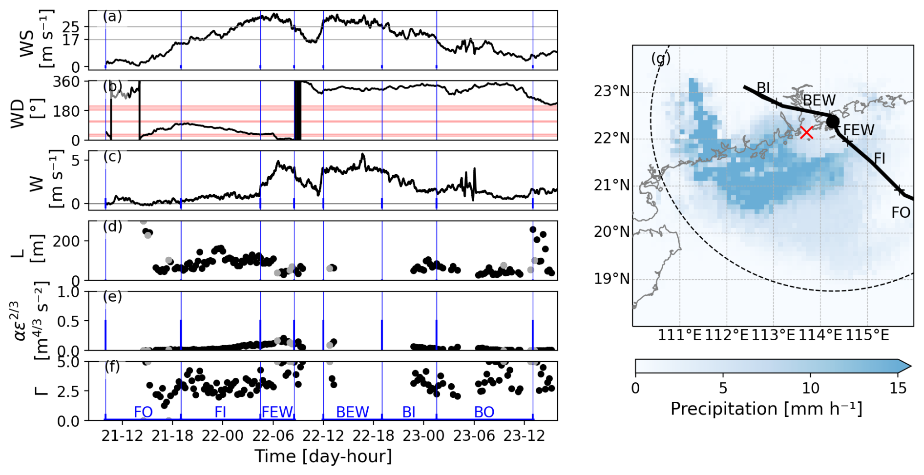
Figure 5 (a–c) Measured wind field at 60 m during Typhoon Nuri (10 min running average): (a) horizontal wind speed, (b) wind direction (red shading indicates wind directions, where the innermost 6 km is influenced by land), (c) vertical wind speed, (d–f) fitted Mann parameters (cases in which one of the fitted parameters equals the prescribed parameter limits are shown in gray), (g) typhoon track from IBTrACS (solid black line, from southwest to northeast), measurement station (red cross), precipitation at 23:00 UTC on 16 August from IMERG (shading), cyclone center at that time (black point), and 400 km distance to cyclone center (dashed black line). Typhoon regions further analyzed are marked in panels (f) and (g): front outer cyclone (FO), front inner cyclone (FI), front eyewall (FEW), back eyewall (BEW), back inner cyclone (BI), and back outer cyclone (BO).

The measurements during Typhoon Nuri show a similar pattern with increasing wind speeds towards the front and back eyewall, separated by a drop in wind speeds (see Fig. 5). In contrast to Hagupit, Nuri's center/track did not move directly over the measurement location (see Fig. 5g). Accordingly, the drop in wind speed is less drastic than during Typhoon Hagupit. At the closest point to the center, the station was at the inner flank of the eyewall (at 10:00 UTC on 22 August 2008). The wind speed around this time is decreased compared to the eyewall winds before and after it. However, as the cyclone center stayed northward of the station, the wind direction did not reverse. At the same time, the measurement time series covers a longer period in the eyewalls and inner-cyclone region than for Hagupit. The horizontal and vertical winds fluctuated around 04:00 UTC on 23 August. This may be associated with the presence of convective cells inside the typhoon. However, precipitation is not as clearly indicated as in the case of Hagupit in the IMERG dataset (not shown).

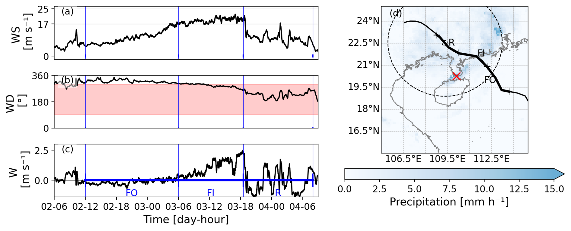
Figure 6 (a–c) Measured wind field at 60 m during Typhoon Prapiroon (10 min running average): (a) horizontal wind speed, (b) wind direction (the red shading indicates wind directions, where the innermost 6 km is influenced by land), (c) vertical wind speed, (d) typhoon track from IBTrACS (solid black line, from southwest to northeast), measurement station (red cross), precipitation at 02:30 UTC on 4 August from IMERG (shading), cyclone center at that time (black point), and 400 km distance to cyclone center (dashed black line). Typhoon regions further analyzed are marked in panels (c) and (d): front outer cyclone (FO), front inner cyclone (FI), and rainband (R).

Measurements during Typhoon Prapiroon (Fig. 6) do not contain information about the eye, as the track is far away from the site (about 160 km). Between 12:00 UTC on 2 August and 18:00 UTC on 3 August 2006, the horizontal and vertical wind speed at the measurement location gradually increased with time, while the typhoon center moved closer to the station. From 18:30 UTC on 2 August onward, the wind field is characterized by fluctuations in wind speed, wind direction, and between up- and downdrafts. We assume that these fluctuations are produced by convection and rain cells within a rainband. This is confirmed by the rain in the IMERG dataset over the station at 02:30 UTC (Fig. 6d).

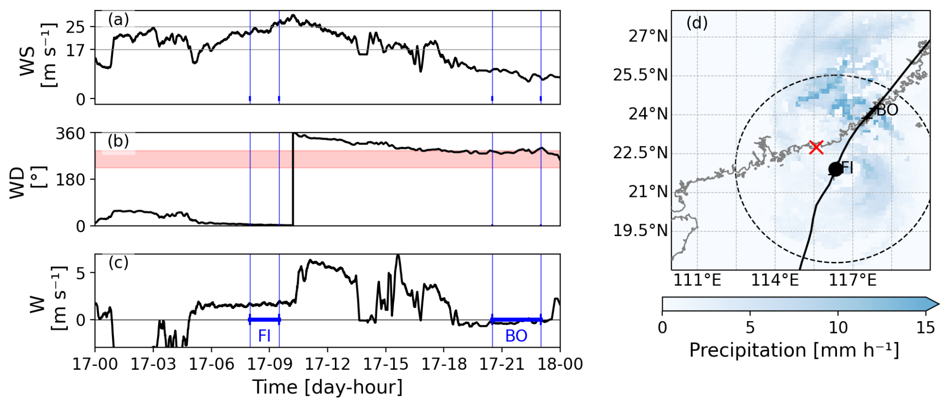
Figure 7 (a–c) Measured wind field at 60 m during Typhoon Chanchu (10 min running average): (a) horizontal wind speed, (b) wind direction (red shading indicates wind directions, where the innermost 6 km is influenced by land), (c) vertical wind speed, (d) typhoon track from IBTrACS (solid black line, from southwest to northeast), measurement station (red cross), precipitation at 09:00 UTC on 17 May from IMERG (shading), cyclone center at that time (black point), and 400 km distance to cyclone center (dashed black line). Typhoon regions further analyzed are marked in panels (c) and (d): front inner cyclone (FI) and back outer cyclone (BO).

Typhoon Chanchu approached the station from the southwest in May 2006 (see Fig. 7). Similar to the case of Prapiroon, the long distance between the measurement station and the typhoon track results in the absence of eye information in the measurements. The measured horizontal wind speed is the largest around 10:00 UTC on 17 May. This was when the cyclone center was closest to the measurement station, which is around 100 km southeast of the station. A large part of the measurements contain prolonged periods with constant values for wind speed, which indicates poor data quality, and the data are therefore not suitable for analyzing turbulence. Yet, two periods with good measurement quality could still be identified and extracted. The first period is in the inner-cyclone region at 09:00 UTC on 17 May, when the cyclone center was about 120 km to the southeast of the measurement mast. This time step is shown in Fig. 7d. The second period, at around 21:00 UTC, covers the outer-cyclone region after the landfall of Typhoon Chanchu.

3.2 The Mann model parameters

For the 30 min periods of measurements that fulfill the criteria described in Sect. 2.1.1, we calculate the spectra and fit the Mann model parameters, as described in Sect. 2.1.2 and 2.2. Here, we first describe the parameter range we obtained by the fitting and how it varies between the tropical cyclone cases and regions. Thereafter, we discuss the goodness of the fit and special features of the spectra. The resulting Mann model parameters for typhoons Hagupit and Nuri are shown in Figs. 4d, e, and f and 5d, e, and f, for L, $\mathit{\alpha }{\mathit{ϵ}}^{\mathrm{2}/\mathrm{3}}$, and Γ, respectively. The corresponding subplots for typhoons Chanchu and Prapiroon are provided in Appendix B. The obtained parameters are further summarized in Table 2 for all four typhoons. Therein we list the median values of these parameters for the specified tropical cyclone regions (see Sect. 2.3) and the sample size per region. Note that for a few 30 min periods, the fitting algorithm resulted in a Mann model parameter equaling the upper or lower bound of the specified parameter range (see Sect. 2.2). In these cases, the fit to the model was poor, suggesting that the fitting algorithm may not have converged. Therefore, these cases were excluded from the calculation of the median Mann model parameters shown in Table 2. The corresponding Mann model parameters are shown in gray in Figs. 4f–g and 5f–g and Figs. B1a–c and B2a–c.

Table 2 Summary of the different analyzed regions for the four typhoon cases. “Fetch” indicates whether the wind comes from the land or from the sea, and “no. samples” gives the number of samples analyzed in each region. Median values are given for wind speed (WS) and the Mann model parameters L, $\mathit{\alpha }{\mathit{ϵ}}^{\mathrm{2}/\mathrm{3}}$, and Γ.

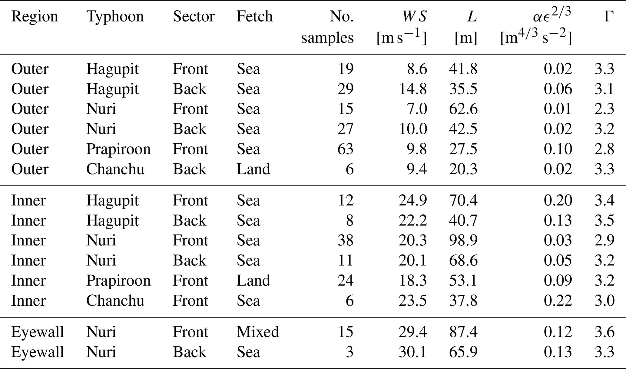
First, we examine the range of the L parameter, which correlates with the size of the largest eddies. Across the four typhoons, the median L values obtained in the different regions range from 20.3 to 98.9 m (see Table 2). L is the largest for Typhoon Nuri. Note that the measurements for Typhoon Nuri were taken from a tower with a base height of 93 m, placing the ultrasonic anemometer at 153 m above sea level. This absolute height is larger than that of the other three typhoon cases, which could explain the larger L values from Nuri compared to the other typhoons. Larger L values could also relate to more unstable atmospheric conditions (Peña et al., 2010a; Sathe et al., 2013).

In all four typhoon cases, the L values in the front sectors before the storm center passed the station are larger than those in the corresponding back sectors. However, the overall L values from these four typhoons are comparable to those obtained in non-typhoon conditions during neutral stratification at similar measurement heights in Høvshore and Østerid (Denmark) (Peña et al., 2010a; Peña, 2019).

For the four typhoon cases, $\mathit{\alpha }{\mathit{ϵ}}^{\mathrm{2}/\mathrm{3}}$ varies between different cyclone regions (see Figs. 4e and 5e). The smallest $\mathit{\alpha }{\mathit{ϵ}}^{\mathrm{2}/\mathrm{3}}$ values are obtained from the spectra in the outer-cyclone region, and the largest $\mathit{\alpha }{\mathit{ϵ}}^{\mathrm{2}/\mathrm{3}}$ values are obtained from those of the inner-cyclone and eyewall regions, suggesting more efficient dissipation at stronger winds. This variation in $\mathit{\alpha }{\mathit{ϵ}}^{\mathrm{2}/\mathrm{3}}$ is related to the variance of the velocity components and the horizontal wind speed. The variance and $\mathit{\alpha }{\mathit{ϵ}}^{\mathrm{2}/\mathrm{3}}$ increase with increasing wind speed, a relation consistent with Sathe et al. (2013). In their study, they find $\mathit{\alpha }{\mathit{ϵ}}^{\mathrm{2}/\mathrm{3}}$ of the order of 0.03 m${}^{\mathrm{4}/\mathrm{3}}$ s⁻² for wind speeds of 7 m s⁻¹ and 0.13 m${}^{\mathrm{4}/\mathrm{3}}$ s⁻² for wind speeds of 16 m s⁻¹ at 90 m during neutral atmospheric stability in Høvshore (Denmark). The median values obtained during the four typhoons range between 0.01 m${}^{\mathrm{4}/\mathrm{3}}$ s⁻² in Nuri's front outer-cyclone region and 0.22 m${}^{\mathrm{4}/\mathrm{3}}$ s⁻² in Chanchu's front inner-cyclone region. The $\mathit{\alpha }{\mathit{ϵ}}^{\mathrm{2}/\mathrm{3}}$ values are smaller for Typhoon Nuri compared to the other typhoon cases at corresponding wind speeds. This is likely because the measurements of Nuri are at an effective height of 153 m compared to about 60 m for the other typhoon cases (see previous paragraph), and for surface-driven turbulence, $\mathit{\alpha }{\mathit{ϵ}}^{\mathrm{2}/\mathrm{3}}$ and the dissipation rate usually decrease with height; see Fang et al. (2023) and also, e.g., Peña (2019) for non-typhoon conditions.

The median Γ values range between 2.3 and 3.6 across the analyzed regions and typhoons, with a median of 3.2 over all regions (see Table 2). This range is comparable to values found in non-typhoon conditions. For instance, the range for Γ is between 3 and 3.5 for neutral conditions at heights between 60 and 100 m at the Høvshore and Østerid sites (Sathe et al., 2013; Peña, 2019).

3.3 How well does the Mann model fit the spectra?

In this section, we summarize when the Mann model can describe the measured spectra and what features it cannot cover. For that, we compare spectra obtained from measurements with the Mann model fit. Figures 8, 9, and 10 show the normalized spectra as a function of wavenumber for the outer-cyclone, the inner-cyclone, and the eyewall regions, respectively. Note that there are a number of 30 min segments for each case (listed in Table 2), and hence the same number of spectra. Here, we show the median of both the measured spectra (solid curves) and the Mann model (dashed curves). The corresponding median Mann model parameters can also be found in Table 2.

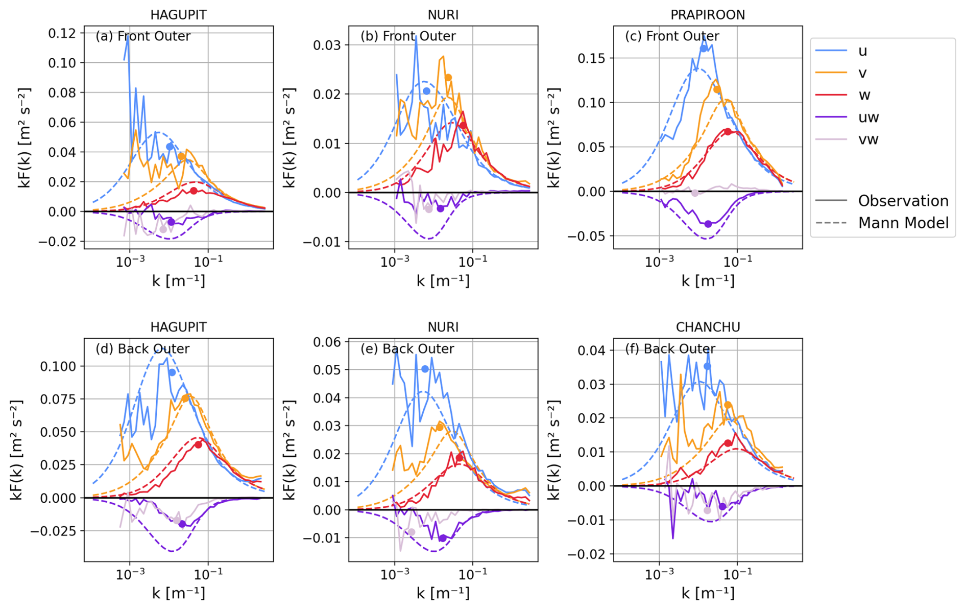
Figure 8 Spectra from the front and back outer-cyclone regions of the four typhoon cases: median of observed spectra (solid lines), fitted Mann model (dashed lines), and estimated maxima of the observed spectra (points).

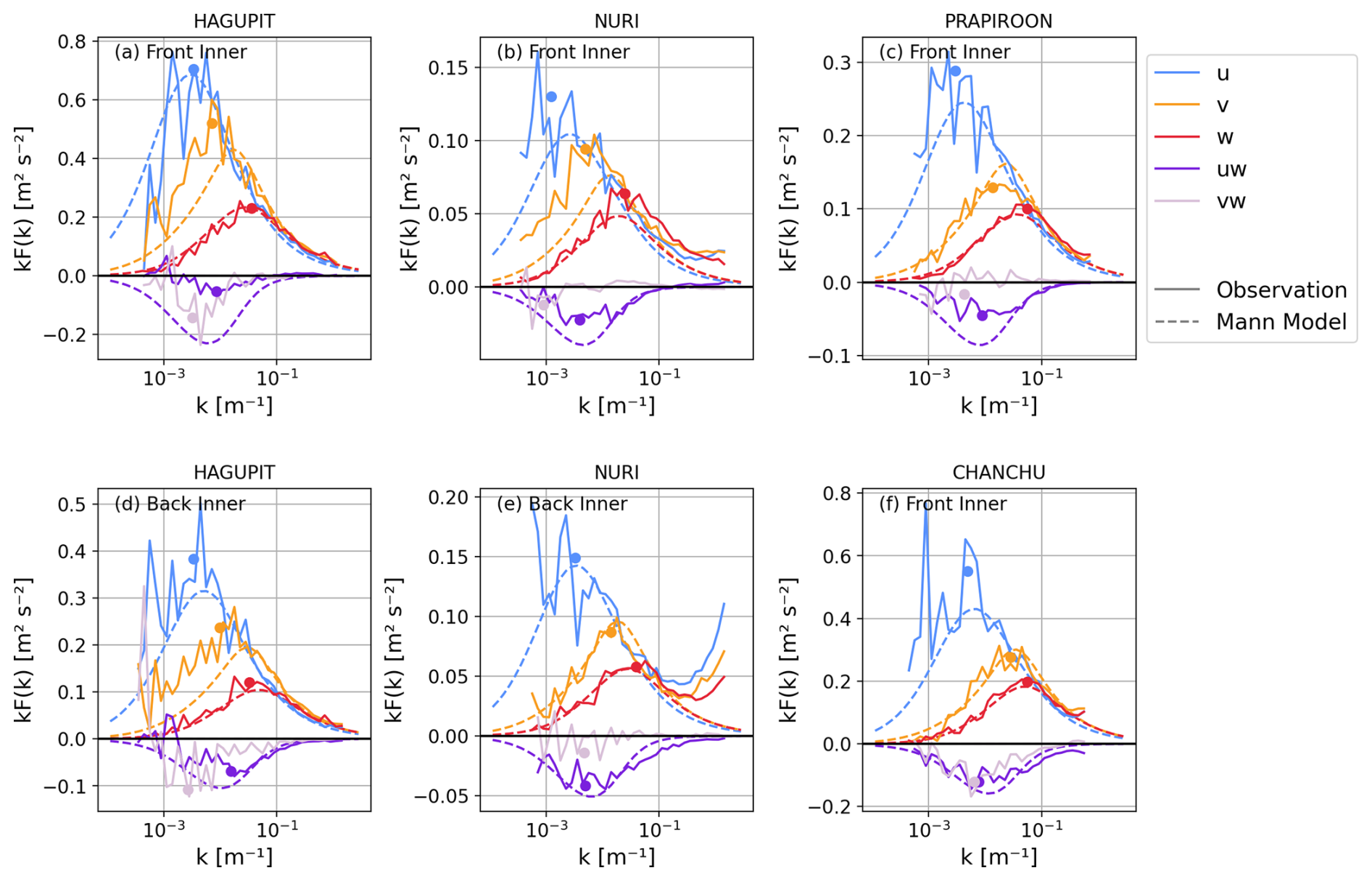
Figure 9 Spectra from the front and back inner-cyclone regions of the four typhoon cases: median of observed spectra (solid lines), fitted Mann model (dashed lines), and estimated maxima of the observed spectra (points).

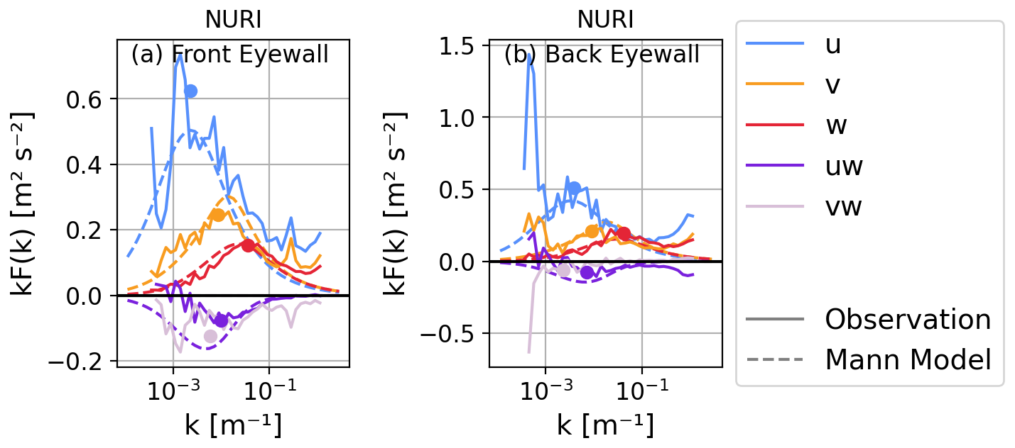
Figure 10 Spectra from the front and back eyewall of Typhoon Nuri: median of observed spectra (solid lines), fitted Mann model (dashed lines), and estimated maxima of the observed spectra (points).

The spectra from measurements resemble the Mann model in several aspects, as listed in the following. This is true not only for the outer region (Fig. 8), but also the inner region (Fig. 9) and eyewall region (Fig. 10). This means that some features covered by the Mann model are, in most instances, also evident in the measured spectra. These features include the fact that (1) the normalized spectra have a maximum at wavenumber k_p, and the normalized spectral energy generally decreases towards larger and smaller wavenumbers; (2) kF_u is larger than kF_v and kF_w at k<k_p; (3) kF_uw is negative, which means that the momentum flux of the u wind component is downward; and (4) k_p is smaller for the u component than for the v component and the largest for the w component. These features are consistent with the usual boundary layer spectra for wind components. However, when zooming in on these features, there are discrepancies between the model and measurements.

Table 3 Comparison between median measured spectra (mes.) and the fitted Mann model (Mann). slope_k1 gives the mean slope of kF_u, kF_v, and kF_w at $k>{\mathrm{10}}^{-\mathrm{1}}$ m⁻¹, and slope_k2 gives the mean slope of kF_u and kF_v at $k<\mathrm{3}\times {\mathrm{10}}^{-\mathrm{3}}$ m⁻¹. The columns k_pF_u(k_p), k_pF_u(k_p), k_pF_u(k_p), and k_pF_uw(k_p) give the normalized spectral power at the peak wavenumber k_p for u, v, and w autospectra and the uw cospectra. $\log \left(\frac{k_{p,v}}{k_{p,u}}\right)$ compares the k_p of the u and v components. Note that large values of slope_k1 could be related to measurement noise.

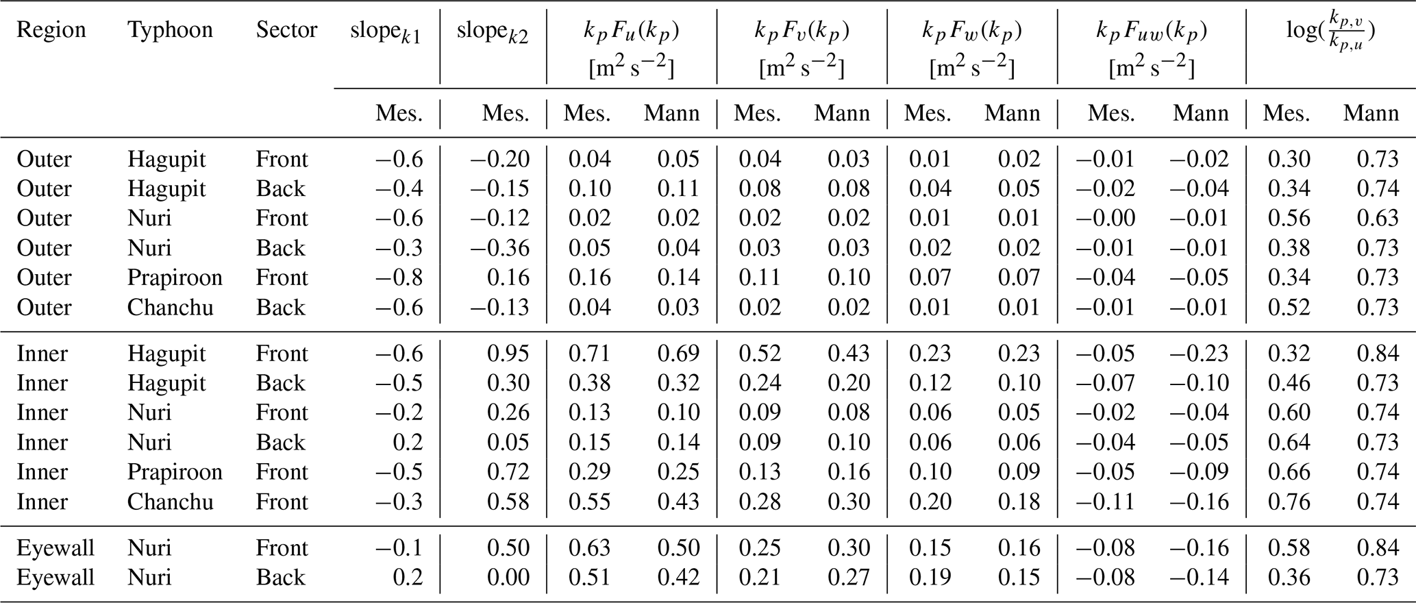
First, we address the slope of the spectra at $k>{\mathrm{10}}^{-\mathrm{1}}$ m⁻¹. This wavenumber range is often referred to as the inertial subrange. In this range, the slope of the normalized spectra on a double logarithmic axis is expected to be $-\mathrm{2}/\mathrm{3}$ in classical boundary layer theory and in the Mann model. Larger slopes can result from measurement noise (Kaimal and Finnigan, 1994). Table 3 lists the slope at $k>{\mathrm{10}}^{-\mathrm{1}}$ m⁻¹ as slope_k1. The slope is obtained from a linear fit to the median of the measured spectra for the different regions and typhoons. For typhoons Hagupit, Prapiroon, and Chanchu, the slope at $k>{\mathrm{10}}^{-\mathrm{1}}$ m⁻¹ is mostly close to or slightly larger than $-\mathrm{2}/\mathrm{3}$. Differently, in Typhoon Nuri's inner-cyclone region and eyewall region, the slope is significantly larger at $k>{\mathrm{10}}^{-\mathrm{1}}$ m⁻¹. This can be seen clearly in Figs. 9e and 10a and b, where the observed spectra show excessive energy at $k\gtrsim {\mathrm{10}}^{-\mathrm{1}}$ m⁻¹. The enhanced energy at $k\gtrsim {\mathrm{10}}^{-\mathrm{1}}$ m⁻¹ could be caused by flow distortions from the meteorological tower (Barthlott and Fiedler, 2003) or tower vibrations (Gao et al., 2024). Nevertheless, using the same measurements, Li et al. (2015) also reported the positive slope in the spectra during Typhoon Nuri. They proposed that the secondary peak in the spectra at these large frequencies (or large wavenumbers, respectively) could be related to the evaporation of sea spray and the associated buoyancy force, as well as coastal roughness changes and surface waves. Also, other studies reported on enhanced spectral energy at high frequencies during typhoon conditions (Tao and Wang, 2019; He et al., 2022). However, this spectral behavior is only obvious during Nuri, and measurement noise cannot be ruled out as a possible cause. More measurements and research are needed to understand the spectral behaviors at $k>{\mathrm{10}}^{-\mathrm{1}}$ m⁻¹, where excessive energy is present.

Second, we investigate the importance of large-scale fluctuations in tropical cyclone turbulence. To do this, we examine the slope of the spectra for $\mathrm{3}\times {\mathrm{10}}^{-\mathrm{3}}$ m⁻¹, which is on the large-scale side of the approximate peak wavenumber. The slopes from the observed u and v spectra at $\mathrm{3}\times {\mathrm{10}}^{-\mathrm{3}}$ m⁻¹ are listed in Table 3 as slope_k2. The corresponding slope of the u and v components from the Mann model fitted to the spectra is of the order of 0.6 (not shown). In five out of six cases in the outer-cyclone regions, the slope in the observed spectra is negative. This is evident in Fig. 8a, b, d, e, and f, where there is larger spectral energy than predicted by the Mann model at small wavenumbers, e.g., $k\simeq {\mathrm{10}}^{-\mathrm{3}}$ m⁻¹ in the observed spectra compared to the Mann model. The small slope in these spectra suggests the presence of significant large-scale wind fluctuations that are beyond the concept of the Mann model. We discuss this feature in more detail in Sect. 4. The slope at $\mathrm{3}\times {\mathrm{10}}^{-\mathrm{3}}$ m⁻¹ is mostly larger and in better agreement with the Mann model in the inner-cyclone and eyewall regions shown in Figs. 9 and 10 compared to the outer-cyclone region.

Third, we examine one of the key spectral parameters, the peak wavenumber k_p and the corresponding energy k_pF(k_p) in Figs. 8–10, from both the measurements and the Mann model. For the Mann model curve, it is straightforward to find k_p and the corresponding k_pF(k_p). For measurements, we decide k_p through visual inspection, as there is often enhanced and fluctuating kF(k) for $k<{\mathrm{10}}^{-\mathrm{3}}$ m⁻¹, which makes it difficult to find an objective k_p. For reference, the obtained maxima are marked as points in Figs. 8–10 together with the median values of the spectra. Table 3 lists the obtained k_pF(k_p) for the measurements and Mann model. In most cases, k_pF_u(k_p), k_pF_v(k_p), and k_pF_w(k_p) from the fitted Mann model are close to those of the measured spectra. However, particularly in the inner-cyclone region (Fig. 9), there are cases where the Mann model underestimates k_pF_v(k_p). This is clearly visible in Fig. 9a, b, and d, which show the front inner-cyclone region of Hagupit and Nuri and the back inner-cyclone region of Hagupit. In these three cases, the Mann model seems to have captured the v variability in smaller eddies, while it missed out on the low wavenumber variability. At the same time, k_p of the v component is overestimated in the Mann model or, in other words, shifted to larger wavenumbers compared to the measurements. This is not the case for k_p of the u component, for which the Mann model performed better overall. In other words, the dominating eddy sizes for u and v are significantly closer to each other in measurements than the Mann model suggests. We summarize this quantity as $\log (k_{p,v}/k_{p,u})$ in Table 3. From the values, it is evident that this feature is consistent in 13 out of the 14 observed spectra in the different regions and typhoons. This agrees with the findings of Zhang et al. (2011): they found that the k_p values of the u and v components are closer to each other in the spectra observed in tropical cyclones than in the turbulence models from Kaimal et al. (1972) and Miyake et al. (1970).

Fourth, we find that the Mann model overestimates the magnitude of kF_uw for k≤k_p. This is evident in Figs. 8–10, as well as from the estimated k_pF_uw(k_p), listed in Table 3. Such an overestimation of kF_uw has also been observed over Denmark, i.e., in areas not affected by tropical cyclones (Peña et al., 2010b; Peña, 2019). Non-negligible negative values are found in kF_vw in 10 out of the 14 regions. While such significant $u^{\prime }{w}^{\prime }$ covariances are not accounted for in the Mann model, they have been observed at moderate to high wind speeds in offshore and coastal environments under non-tropical-cyclone conditions (e.g., Geernaert, 1988).

4 Discussion

In this study, sonic anemometer measurements covering four tropical cyclones are analyzed. While the collection of these data is far from rich, it offers several opportunities. First, although the Mann model is well established in the wind energy sector, it has been tested for tropical cyclone conditions in only a few studies and without detailed analysis. Second, the data analyzed include situations where the measurement stations experience a variety of typhoon structures, here called “regions” and illustrated in Fig. 1, including the eye, eyewall, rainband, inner-cyclone, and outer-cyclone regions. Thus, this study addresses the turbulence spectral behavior in different parts of a typhoon and the corresponding Mann model performance.

We note that the data cover only four typhoons. Due to the limited number of typhoons covered in this study, and further complicated by the data quality and the division into regions based on the cyclone structure, the number of samples for each region is severely limited. Therefore, the results of this study cannot be generalized for turbulence characterization for the different regions within a typhoon. Nevertheless, the data were valuable for examining turbulence characteristics under typhoon conditions and for assessing the Mann model in this context.

Our analysis provided important insights into the variability at lower wavenumbers ($k\lesssim \mathrm{3}\times {\mathrm{10}}^{-\mathrm{1}}$ m⁻¹) within typhoons. In particular, we found that, in the outer-cyclone region, both u and v can have larger spectral energy than predicted by the Mann model at lower wavenumbers; see Fig. 8. This is clearly shown by the smaller slope of the spectra at $\mathrm{3}\times {\mathrm{10}}^{-\mathrm{1}}$ m⁻¹ compared to the Mann model (slope_k2 in Table 3). Similarly, larger-than-predicted spectral energy at low wavenumbers has been reported in several studies in offshore environments under non-tropical-cyclone conditions (De Maré and Mann, 2014; Cheynet et al., 2018). The present analysis demonstrates that this also applies to tropical cyclones. The large energy content at these lower wavenumbers in the outer-cyclone region is likely related to significant mesoscale fluctuations observed in previous studies dealing with turbulence under non-tropical-cyclone conditions (e.g., De Maré and Mann, 2014; Larsén et al., 2019; Syed and Mann, 2024). Ground blockage effects could also lead to a flattened top of the u and v spectra (Mann, 1994), evident for example in the back outer region of Typhoon Chanchu (Fig. 8f). One of the implications of the large spectral energy at lower wavenumbers is that using a 30 min window of the time series may not be long enough; this is consistently suggested in all six subplots of Fig. 8, as there is a high energy level at the lowest wavenumber, even for the relatively well-behaving spectra from the front outer region of Typhoon Prapiroon. In the spectra of the outer-cyclone region, the width of the energy-containing range is broad, thus containing a broad-scale range of active turbulence contributors. This width is considerably narrower in the inner-cyclone and eyewall regions shown in Figs. 9 and 10, likely due to the better-defined convection-driven turbulence in these regions. Nonetheless, the high energy level at the lowest wavenumber also suggests that the 30 min time series is not long enough for turbulence estimation.

To better understand the sources of variability at lower wavenumbers, we examined the role of boundary layer rolls. These rolls have been observed in various flow situations over land and the ocean (Kosović et al., 2026). The following discussion is motivated by the fact that boundary layer rolls are also often present during tropical cyclone events (Zhang et al., 2008; Huang et al., 2018; Tang et al., 2021). Smedman (1991) studied the turbulence behavior associated with boundary layer rolls for a case over the Baltic Sea using turbulence measurements from a 145 m meteorological tower. Although the flow situation analyzed in their study differs from that in typhoons, it is likely that boundary layer rolls have a similar impact on turbulence. In their study, they found excessive spectral energy in the v and w components at low frequencies (around 0.003 Hz) and countergradient $v^{\prime }{w}^{\prime }$ fluxes. Larger spectral energy than that predicted by the Mann model in the v component was also observed in three of the four typhoons in our analysis. To see if this could be related to the boundary layer rolls or other organized structures, we simulate the four typhoons with the Weather Research and Forecasting (WRF) model (version 4.51) (Skamarock et al., 2019a). The simulation uses four one-way nested domains, with a horizontal grid spacing of 18, 6, 2, and $\mathrm{2}/\mathrm{3}$ km. Refer to the Appendix C for more details on the simulation setup. It should be noted that a spatial resolution of $\mathrm{2}/\mathrm{3}$ km in the WRF simulation does not resolve all the wind variability associated with structures such as boundary layer rolls. Nevertheless, the model output is expected to be helpful in identifying the presence or absence of these associated patterns (Svensson et al., 2017). We observe the presence of roll-like patterns in the simulations of typhoons Hagupit and Nuri close to the corresponding measurements. Roll patterns are also present during Chanchu and Prapiroon, but they are far away from the measurement station during the analyzed time periods.

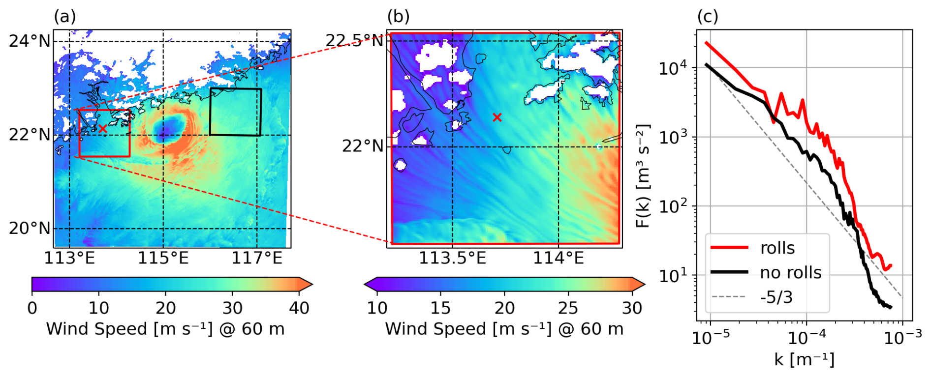
Figure 11 (a, b) Simulated horizontal wind speed during Typhoon Nuri at 60 m above sea level. Panel (b) shows a detailed view of the area marked in red in panel (a); note the different color scales. The red cross in panels (a) and (b) gives the measurement location, and the black contours give the coastlines. White areas have a terrain elevation larger than 60 m. (c) Wind speed power spectra calculated from the simulated wind speed at 60 m from the areas marked in red and black in panel (a), representing areas with and without boundary layer rolls. The dashed line gives a slope of $-\mathrm{5}/\mathrm{3}$ for reference.

To illustrate these patterns, Fig. 11a and b show the simulated wind field from the innermost model domain at a height of 60 m at 03:00 UTC on 22 August 2008 during Typhoon Nuri. Note that the cyclone center was observed to be at 21.8° N, 114.7° E at that time (Knapp et al., 2010; Gahtan et al., 2024), whereas the simulated cyclone center is offset by around 35 km to the northeast (see the area with small wind speeds around 22° N, 115° E in Fig. 11a). Figure 11b provides a closer look at the area around the measurement site (marked in red). In this area, the boundary layer rolls can be seen as elongated bands of alternating above- and below-average horizontal wind speeds, circulating around the cyclone center. Near the measurement site, the rolls are in a northwest–southeast orientation; see Fig. 11b. At this time, the cyclone flow from the north had passed the upwind land areas, which modified the wind field. There are also other examples of similar roll structures appearing far from land in the simulations (not shown). The vertical wind speed has a similar structure to the horizontal wind, with elongated bands of upward and downward motion, respectively (not shown). To demonstrate the excessive energy associated with these organized wind features, we compute and compare the wind speed power spectra from regions with and without roll structures from the simulations (see Appendix C for details). The spectra for the area with rolls and for an area without visible boundary layer rolls are shown in Fig. 11c. The spectrum from the area with rolls shows enhanced energy over all scales, especially in the range from $k\sim \mathrm{5}\times {\mathrm{10}}^{-\mathrm{5}}$ to $\mathrm{8}\times {\mathrm{10}}^{-\mathrm{4}}$ m⁻¹, which corresponds approximately to a wavelength of 1 to 20 km. Note that these scales are larger than those shown in Figs. 8–10. In reality, boundary layer rolls likely influence those smaller scales as well. However, the ability of the WRF simulations to represent this variability is limited by the model resolution. With the $\mathrm{2}/\mathrm{3}$ km horizontal grid spacing, the effective resolution of the simulations is of the order of 5 km (Skamarock, 2004). Consequently, wind variability at wavenumbers larger than $k>\mathrm{2}\times {\mathrm{10}}^{-\mathrm{4}}$ m⁻¹ cannot be fully resolved. Furthermore, previous studies have shown that the simulated roll wavelength decreases with increasing horizontal resolution in mesoscale models (Svensson et al., 2017). In tropical cyclones, boundary layer roll structures are found to have wavelengths of the order of 0.6–1.5 km based on synthetic aperture radar (SAR) (Morrison et al., 2005; Zhang et al., 2008; Huang et al., 2018), which is smaller than in the WRF simulations.

To conclude the discussion on the role of organized atmospheric features, the simulations suggest that boundary layer rolls were present in Nuri's front inner region (Fig. 11), in Hagupit's front outer-cyclone region, and in Hagupit's front inner-cyclone region (not shown). The corresponding spectra calculated from the measurements all show enhanced energy in the crosswind component at $k\gtrsim \mathrm{3}\times {\mathrm{10}}^{-\mathrm{2}}$ m s⁻¹ compared to the Mann model (Figs. 8a and 9a, b). This supports the hypothesis that the excessive energy in kF_v(k) at small wavenumbers could be associated with the roll-like structures inside the typhoons. However, more research with more data is needed to further support this hypothesis.

In the next part of the discussion, we need to address the uncertainties associated with the spectral analysis of the measurements, apart from the small number of data samples mentioned earlier in this section. During the passage of a typhoon, the changes in both wind speed and wind direction can be significant, challenging the validity of the stationarity assumption. This is also one of the reasons why we limited the length of the time series to 30 min, rather than using longer periods. These changes in wind speed and direction challenge the analysis in terms of (1) decomposing the wind vector into the u and v components and using the Taylor frozen hypothesis to convert spectra from the frequency domain to the wavenumber domain and (2) taking the average spectra of the typhoon regions defined in Sect. 2.3. Limitations of these two points are discussed in the following. We have assessed whether the decomposition of the wind vector into its u and v components is successful or not by calculating and comparing the spectra of u with those of the wind speed. A successful decomposition would result in more or less the same spectra for wind speed and the u component. This is the case in our study, which gives credit to the analysis of the u and v components of the turbulence spectra. Note that we did not analyze the data in the eye of Typhoon Hagupit due to the non-stationary time series. As described in Sect. 2.3, our analyses are mainly based on the median value of the spectra obtained within defined typhoon regions. Due to the large-scale typhoon structure, the wind and turbulence properties are expected to be associated with these regions. Therefore, the analysis is expected to be sensitive to the definition of each region. Given the complex spatial structure of a constantly evolving and moving tropical cyclone, our definition may be an oversimplification. Furthermore, when comparing the median spectra from measurements with the Mann model, we used the median of the L, $\mathit{\alpha }{\mathit{ϵ}}^{\mathrm{2}/\mathrm{3}}$, and Γ parameters. In general, these parameters are different from those obtained by fitting the Mann model to the median spectra.

In addition, spatial coherence also has a known impact on wind turbine loads (Davenport, 1961; Dimitrov et al., 2017). The coherence resulting from the Mann model depends on the L and Γ parameters. For non-typhoon conditions, measurements indicate that the coherence of the u component is overestimated for vertical separations (Mann, 1994; Cheynet, 2019). However, whether this is also the case for tropical cyclone conditions is beyond the scope of the current study. Further studies are needed for such an investigation.

Finally, we discuss the use of the Mann model for generating stochastic wind field inputs for aeroelastic wind turbine load simulations. The Mann model generates horizontally homogeneous, stationary turbulence fields and is well suited for load assessments under quasi-steady atmospheric conditions. Traditionally, aeroelastic simulations are run for 10 min periods, which is often a reasonable assumption for turbulence in the atmospheric surface layer. However, particularly under offshore conditions and above the surface layer, significant spectral energy is often observed at timescales of several tens of minutes (e.g., De Maré and Mann, 2014; Larsén et al., 2019), and longer time series are required to capture the associated larger turbulent eddies. This behavior is also observed for the typhoon cases analyzed here. This poses a fundamental difficulty, as the assumption of stationarity over 10 min, or even longer intervals, is problematic in tropical cyclones. This is evident in the rapid increase in wind speed within the front eyewall region and the pronounced changes in wind direction during eye passage. Notably, despite the non-stationarity, the turbulence does not deviate strongly from Gaussian behavior, in agreement with Cao et al. (2009); across all analyzed 30 min segments, the median skewness and kurtosis are 0.0 and 2.9, respectively. While stationary turbulence models, such as the Mann model, capture key statistical properties of turbulence, they are not designed to represent the non-stationary nature of tropical cyclones at timescales of 10 min and longer. In bridge engineering, several non-stationary frameworks have been developed to analyze tropical cyclone turbulence and to generate synthetic, time-varying wind fields (Xu and Chen, 2004; Wang et al., 2018; Tao and Wang, 2019). Related approaches that incorporate mesoscale fluctuations have also been explored in the wind energy sector, for example by Syed and Mann (2024). Further research in this direction could benefit from incorporating methodologies developed in both the wind energy and the civil engineering communities.

5 Conclusions

Turbulence during tropical cyclone conditions is a less studied topic in the context of wind energy (e.g., Kosović et al., 2026). However, it is becoming increasingly important with the rapid development of wind energy in cyclone-prone regions. Accurate estimation of turbulence is important for safer operation and design of wind turbines. This study investigates how well the uniform Mann shear model describes typhoon turbulence and what limitations the model may have. The Mann model is one of the turbulence models recommended by the IEC standard that can be used to simulate three-dimensional wind fields, as is necessary, for example, for load calculations. The study is conducted by analyzing sonic anemometer measurements from four stations, where four typhoons from 2006 to 2008 passed by, with the eye of one of the typhoons passing over the station and the eyes of the other typhoons passing within a few hundred kilometers of the respective stations. The data were sorted into different regions inside a typhoon structure: the outer region, inner region, eyewall, eye, and rainbands. We fitted the spectra calculated from the measurements to the Mann model and assessed how well the model describes the spectral behaviors during tropical cyclone conditions in different cyclone regions.

The analysis revealed that it is difficult to apply the Mann model to the eye and rainbands due to the non-stationarity of the wind field in these regions. In the outer-cyclone, inner-cyclone, and eyewall regions, the Mann model fit the tropical cyclone power spectra relatively well in some cases. However, clear discrepancies were found between the observed spectra and the model, primarily concerning the following:

1. In the outer-cyclone region, the slope of the observed spectra at $k<\mathrm{3}\times {\mathrm{10}}^{-\mathrm{3}}$ m⁻¹ is, for three out of four typhoon cases, significantly smaller than that predicted by the Mann model. This corresponds to a relatively broad energy-containing range with multiple peaks and a flatter spectral top, suggesting the presence of large-scale wind fluctuations. While the Mann model is generally able to capture one of the peak modes on the microscale, it fails to represent most of the large-scale fluctuations. This feature compares qualitatively to findings made in offshore conditions unaffected by tropical cyclones (De Maré and Mann, 2014; Cheynet et al., 2018). We note that estimates of the power spectra based on a limited sample size are inherently subject to uncertainty, particularly at the smallest wavenumbers.

2. In the inner-cyclone region and eyewalls of Typhoon Nuri, larger spectral energy is found at $k>{\mathrm{10}}^{-\mathrm{1}}$ m⁻¹ compared to the Mann model. Whether this large spectral energy is related to tower vibration, tower shadowing, or other measurement-quality-related issues could not be verified with the available data. Nevertheless, it has been argued by Li et al. (2015) that the large spectral energy at these small scales during typhoons may be related to sea spray evaporation, surface roughness changes, and waves. Clearly, more measurements are required to address such a hypothesis.

3. In the inner-cyclone region, significantly enhanced spectral energy is found in the crosswind component of Typhoon Nuri and Hagupit at $k\lesssim {\mathrm{10}}^{-\mathrm{2}}$ m⁻¹ compared to the Mann model. At the same time, the peak wavenumbers of the u and v spectra are closer to each other than the Mann model suggests.

4. Further deviations of the Mann model in the uw and vw cospectra have previously been reported under non-tropical-cyclone conditions. These deviations are also evident in the analyzed typhoon cases: the Mann model overestimates energy in the uw cospectra, consistent with findings from different sites in Denmark (Peña et al., 2010b; Peña, 2019). Further, in contrast to the Mann model, non-negligible energy is observed in the measured vw cospectra. This has previously been reported for coastal regions under non-tropical-cyclone events (e.g., Geernaert, 1988).

As listed above, one of the striking characteristics of typhoons is the spectral behaviors related to the crosswind component v. The current study addresses this by relating it to the often-present boundary rolls inside tropical cyclones using both measurements and numerical simulation. Our study suggests a positive linkage between the excessive energy in the v component and the presence of boundary layer rolls.

We acknowledge that turbulence is highly variable during tropical cyclones and is case dependent. Further studies based on larger datasets should be conducted for more robust results. This study can serve as a reference when investigating tropical cyclone conditions, particularly for structural engineering purposes.

Appendix A: Details and additional illustration to Sect. 2.1.1, data preprocessing

As described under point 2 in Sect. 2.1.1, an algorithm is used to identify spikes in the typhoon measurements. The algorithm is detailed in the following. The spike-detection algorithm closely follows the method proposed by Vickers and Mahrt (1997), specifically their Sect. 6a. However, following Leys et al. (2013), a moving-median absolute deviation (MAD) filter is used instead of the moving-average-based filter originally proposed in Vickers and Mahrt (1997). The MAD is defined as

$$\begin{array}{}\text{(A1)}& \mathrm{MAD}=\mathrm{median}\left(b\left|x_i-\mathrm{median}\left(X\right)\right|\right),\end{array}$$

where x_i is the individual observation in the sample X, and the scaling constant b=1.4826 ensures that the MAD equals the standard deviation for a Gaussian distribution. In the algorithm, the MAD is computed for moving windows of 5 min. Observations whose absolute deviation from the moving median exceed 4× MAD are classified as spikes, unless this occurs for more than three consecutive observations. Identified spikes are replaced using linear interpolation. Any 5 min interval containing more than 5 % spikes is dropped. The thresholds of 4× MAD and 5 % spikes are based on manual inspection of the data. An example is shown in Fig. A1, together with examples of periods filtered because of repeating and alternating values. The latter are identified as described under points 3 and 4 in Sect. 2.1.1.

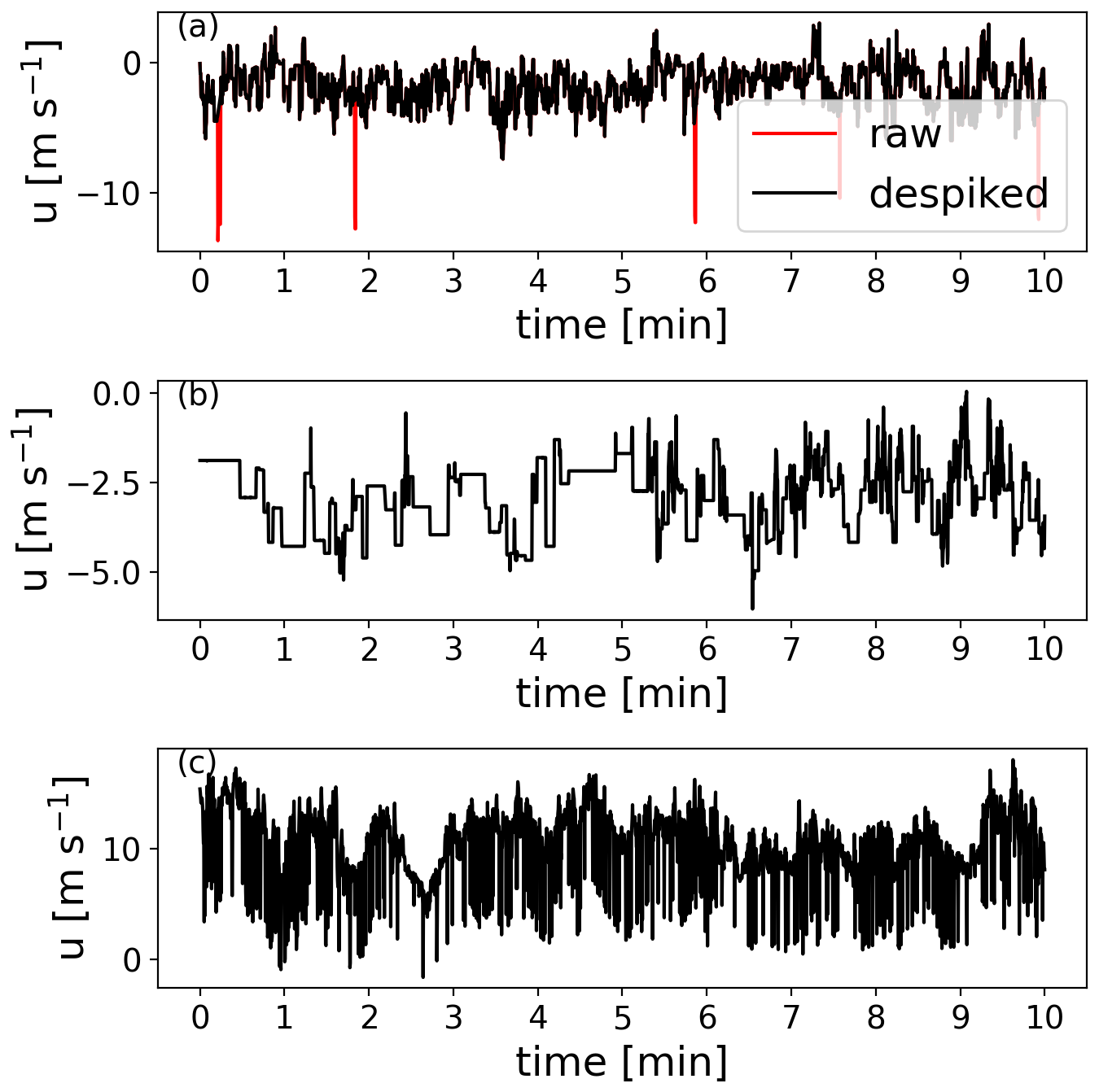
Figure A1 Illustration of data preprocessing: 10 min example periods of west–east wind component during Typhoon Chanchu. (a) Measurements after filtering of spikes (black), with identified spikes (red); (b) measurement period excluded from analysis due to repeated values; and (c) measurement period excluded due to alternating values.

Appendix B: Mann model parameters for typhoons Chanchu and Prapiroon

Figures B1 and B2 show the Mann model parameters for typhoons Prapiroon and Chanchu, respectively. Figures B1a–c and B2a–c are analogous to Figs. 4d–f and 5d–f.

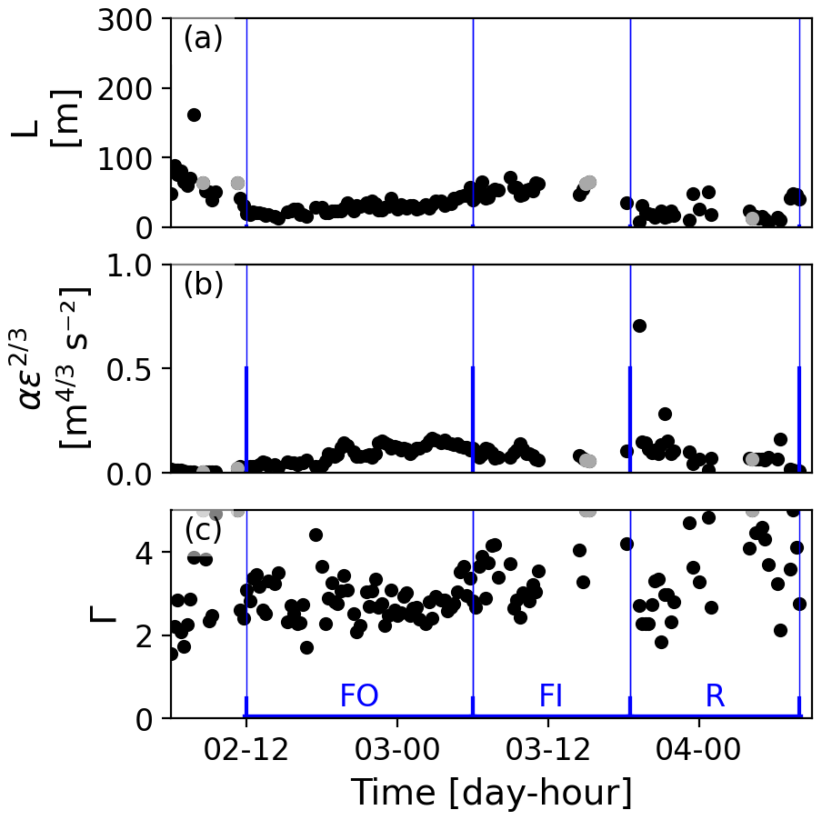
Figure B1 Mann parameters obtained for Typhoon Prapiroon (cases in which one of the fitted parameters equals the prescribed parameter limits are shown in gray). Typhoon regions further analyzed are marked in blue: front outer cyclone (FO), front inner cyclone (FI), and rainband (R).

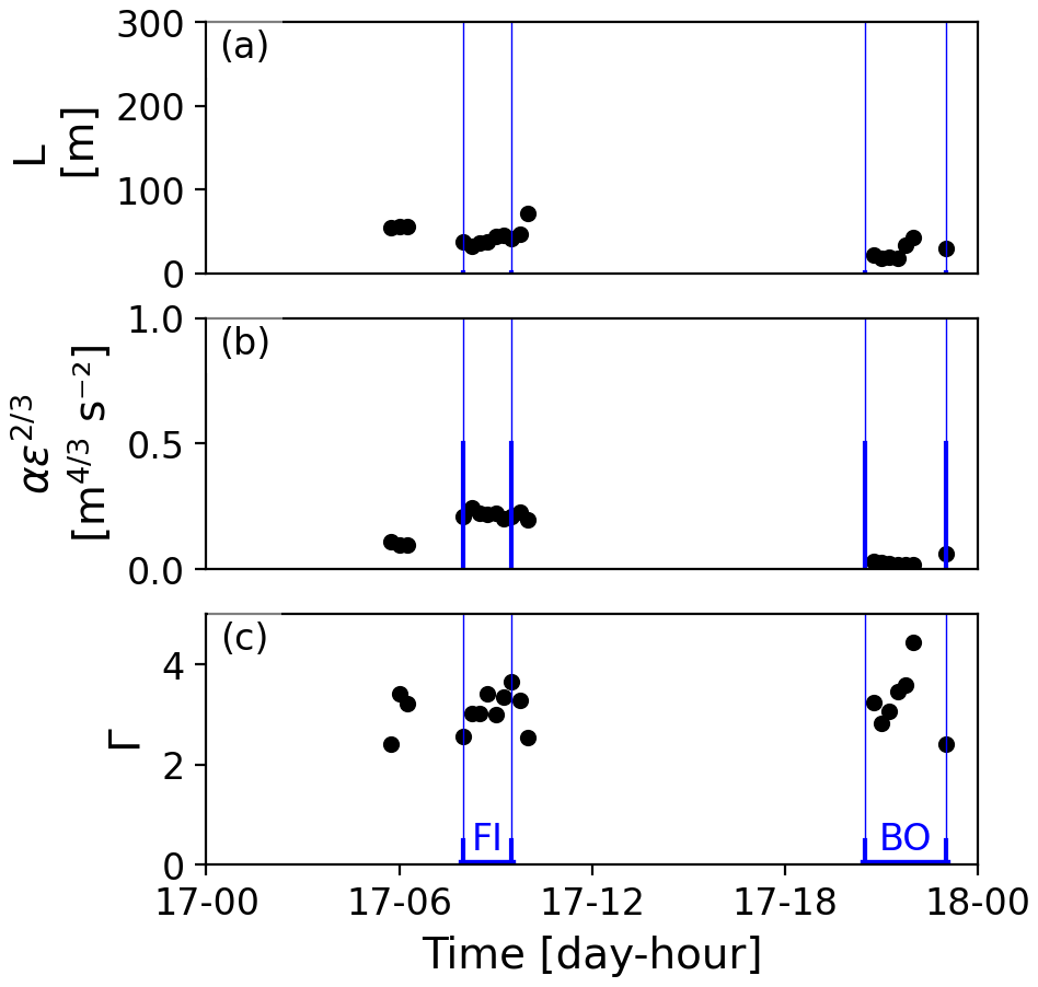
Figure B2 Mann parameters obtained for Typhoon Chanchu. Typhoon regions further analyzed are marked in blue: front inner cyclone (FI) and back outer cyclone (BO).

Appendix C: Simulation setup and calculation of spectra from simulation

Simulations of the four typhoons are performed using WRF version 4.51 (Skamarock et al., 2019b) to analyze the flow structure at and around the measurement locations of the four typhoons. WRF is run on four one-way nested domains, d01, d02, d03, and d04. The outermost domain is d01. The nested domains d02, d03, and d04 are run in a vortex following grid configuration. The horizontal grid spacing is 18, 6, 2, and $\mathrm{2}/\mathrm{3}$ km for d01, d02, d03, and d04, respectively. For the four simulations, d04 has 769 × 769 horizontal grid points. A total of 70 vertical model levels are used, with the lowermost levels at heights around 8, 26, 47, 72, 102, 139, 183, and 292 m. Initial and boundary conditions are taken from ERA5 reanalysis data (Hersbach et al., 2018), and the sea surface temperature is taken from OSTIA (Donlon et al., 2012). The simulations are started at 12:00 UTC on 21 August 2008 for Typhoon Nuri, at 00:00 UTC on 23 September 2008 for Typhoon Hagupit, at 12:00 UTC on 16 May 2006 for Typhoon Chanchu, and at 00:00 UTC on 2 August 2006 for Typhoon Prapiroon. The first 6 simulation hours after the simulation start is used for the model spin-up. The following parameterization schemes are used: the Yonsei University boundary layer scheme (YSU) (Hong et al., 2006), the revised MM5 surface layer scheme (Jiménez et al., 2012) with the isftcflx option 2, the Thompson microphysics scheme (Thompson et al., 2008), the RRTMG radiation scheme (Iacono et al., 2008), and the Kain–Fritsch cumulus scheme (Kain, 2004). The latter is only activated in d01.

To analyze the simulated wind speed fluctuations, we calculate spectra from the simulation output of d04. For that, spectra are first calculated along the model grid rows (oriented approximately in the west–east direction) and the model grid columns (oriented approximately in the south–north direction) (Müller et al., 2024). These spectra are then averaged over grid rows and columns.