the Creative Commons Attribution 4.0 License.
the Creative Commons Attribution 4.0 License.
 | 24 Oct 2018
From wind to loads: wind turbine site-specific load estimation with surrogate models trained on high-fidelity load databases
Nikolay Dimitrov
Mark C. Kelly
Andrea Vignaroli
Jacob Berg
We define and demonstrate a procedure for quick assessment of site-specific lifetime fatigue loads using simplified load mapping functions (surrogate models), trained by means of a database with high-fidelity load simulations. The performance of five surrogate models is assessed by comparing site-specific lifetime fatigue load predictions at 10 sites using an aeroelastic model of the DTU 10 MW reference wind turbine. The surrogate methods are polynomial chaos expansion, quadratic response surface, universal Kriging, importance sampling, and nearest-neighbor interpolation. Practical bounds for the database and calibration are defined via nine environmental variables, and their relative effects on the fatigue loads are evaluated by means of Sobol sensitivity indices. Of the surrogate-model methods, polynomial chaos expansion provides an accurate and robust performance in prediction of the different site-specific loads. Although the Kriging approach showed slightly better accuracy, it also demanded more computational resources.
- Article
(2149 KB) - Full-text XML
- BibTeX
- EndNote


Before installing a wind turbine at a particular site, it needs to be ensured that the wind turbine structure is sufficiently robust to withstand the environmentally induced loads during its entire lifetime. As the design of serially produced wind turbines is typically based on a specific set of wind conditions, i.e., a site class defined in the IEC (2005) standard, any site where the conditions are more benign than the reference conditions is considered feasible. However, often one or more site-specific parameters will be outside this envelope – and disqualify the site as infeasible unless it is shown that the design load limits are not going to be violated under site-specific conditions. Such a demonstration requires carrying out simulations over a full design load basis, which adds a significant burden to the site assessment process.
Various methods and procedures have been attempted for simplified load assessment for wind energy applications. Kashef and Winterstein (1999) and Manuel et al. (2001) use probabilistic expansions based on statistical moments. Simple multivariate regression models of first order are employed by Mouzakis et al. (1999) and Stewart (2016), while in Toft et al. (2016) a second-order response surface is used. Another response surface approach using artificial neural networks is described in Müller et al. (2017). Polynomial chaos expansion (PCE) is employed by Ganesh and Gupta (2013) for blade load prediction, albeit on a very simple structural representation. Teixeira et al. (2017) use a Kriging surrogate model to map the load variations with respect to offshore environmental conditions. Other relevant studies use some of the methodologies that represent specific analysis steps shown in the present work. These include Hübler et al. (2017) where variance-based sensitivity analysis is employed, Yang et al. (2015) where Kriging is used to enable efficient implementation of reliability-based design optimization, and Murcia et al. (2018) where polynomial chaos expansions are used to carry out uncertainty propagation. In the latter, the model training sample is generated using a Monte Carlo (MC) simulation with a quasi-random sequence, a technique that is also employed in Müller and Cheng (2018) and Graf et al. (2016). An alternative to the surrogate modeling approach discussed in this paper could be the load set reduction, as described in, for example, Häfele et al. (2018) and Zwick and Muskulus (2016), which also reduces the number of simulations required. This approach, however, still requires carrying out high-fidelity simulations that leads to using more time for simulation setup, computations, and postprocessing, while with a surrogate model the lifetime equivalent load computation takes typically less than a minute on a regular personal computer. The studies most in line with the scope of the present paper are those by Müller et al. (2017), Teixeira et al. (2017), and Toft et al. (2016). The former two employ advanced surrogate modeling techniques (artificial neural networks and Kriging, respectively); however, the experimental designs are relatively small and with a limited range of variation for some of the variables, and the discussion does not focus on the practical problem of computing lifetime-equivalent site-specific loads. The computation of site-specific lifetime-equivalent design loads is the main focus in Toft et al. (2016), but with a limited number of variables and using a low-order quadratic response surface. The vast majority of the studies employ a single surrogate modeling approach, meaning that it has not been possible to directly compare the performance of different approaches.
In the present work, we analyze, refine, and expand the existing simplified load assessment methods, and provide a structured approach for practical implementation of a surrogate modeling approach for site feasibility assessment. The study aims at fulfilling the following four specific goals:
-
define a simplified load assessment procedure that can take into account all the relevant external parameters required for full characterization of the wind fields used in load simulations;
-
define feasible ranges of variation in the wind-related parameters, dependent on wind turbine rotor size;
-
demonstrate how different surrogate modeling approaches can be successfully employed in the problem, and compare their performance; and
-
obtain estimates of the statistical uncertainty and parameter sensitivities.
The scope of the present study is loads generated under normal power production, which encompasses design load cases (DLCs) 1.2 and 1.3 from the IEC 61400-1 standard (IEC, 2005). These load cases are the main contributors to the fatigue limit state (DLC1.2) and often the blade extreme design loads (DLC1.3) (Bak et al., 2013; Dimitrov et al., 2017). The methodology used can easily be applied to other load cases governed by wind conditions with a probabilistic description. Loads generated during fault conditions (e.g., grid drops) or under deterministic wind conditions (e.g., operational gusts without turbulence) will in general not be (wind climate) site-specific. The loads analysis is based on the DTU 10 MW reference wind turbine (Bak et al., 2013) simulated using the Hawc2 software (Larsen and Hansen, 2012).
2.1 Schematic description
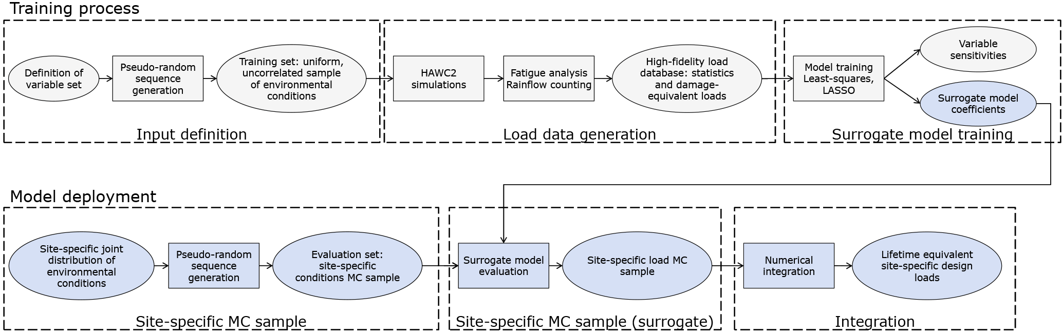
Figure 1 shows a schematic overview of the procedure for site-specific load assessment using simplified load mapping functions (here referred to in general as surrogate models). The main advantage of this procedure is that the computationally expensive high-fidelity simulations are only carried out once, during the model training process (top of Fig. 1). In the model deployment process (bottom of Fig. 1), only the coefficients of the trained surrogate models are used, and a site-specific load evaluation typically takes less than a minute on a standard personal computer.
2.2 Definition of variable space
The turbulent wind field serving as input to aeroelastic load simulations can be fully statistically characterized by the following variables:
-
mean wind field across the rotor plane as described by the
- –
average wind speed at hub height, U;
- –
vertical wind shear exponent, α;
- –
wind veer (change of mean flow direction with height, Δφ);
- –
-
turbulence described via
-
air density ρ;
-
mean wind inflow direction relative to the turbine in terms of
- –
vertical inflow (tilt) angle and
- –
horizontal inflow (yaw) angle .
- –
All the quantities referred to above are considered in terms of 10 min average values. All variables, except the variables defining mean inflow direction, are probabilistic and site-dependent in nature. The mean inflow direction variables represent a combination of deterministic factors (i.e., terrain inclination or yaw direction bias in the turbine) and random fluctuations due to, for example, large-scale turbulence structures or variations in atmospheric stability. Mean wind speed, turbulence, and wind shear are well known to affect loads and are considered in the IEC 61400-1 standard. In Kelly et al. (2014) a conditional relation describing the joint probability of wind speed, turbulence, and wind shear was defined. The effect of implementing this wind shear distribution in load simulations was assessed in Dimitrov et al. (2015), showing that wind shear has importance especially for blade deflection. The Mann model parameters L and Γ were also shown to have a noticeable influence on wind turbine loads (Dimitrov et al., 2017). By definition, for a given combination of L and Γ, the αε2∕3 parameter from the Mann model is directly proportional to (Kelly, 2018; Mann, 1994), and can therefore be omitted from the analysis. The probability density function (pdf) typically used to synthesize time series of velocity components from the Mann model spectra is Gaussian. For a slightly smaller turbine, the NREL (National Renewable Energy Laboratory) 5 MW turbine, the assumption of Gaussian turbulence has been shown to not impact the fatigue loads (Berg et al., 2016). The final list of inflow-related parameters thus reads as (see Table 1 for details)
The loads experienced by a wind turbine are a function of the wind-derived factors described above, and of the structural properties and control system of the wind turbine. Therefore, a load characterization database taking only wind-related factors into account is going to be turbine-specific.
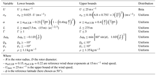
Table 1Bounds of variation for the variables considered. All values are defined as statistics over 10 min reference period.
The variables describing the wind field often have a significant correlation between them, and any site-specific load or power assessment has to take this into account using an appropriate description of the joint distribution of input variables. At the same time, most probabilistic models require inputs in terms of a set of independent and identically distributed (i.i.d) variables. The mapping from the space of i.i.d variables to joint distribution of physical variables requires applying an isoprobabilistic transformation as, for example, the Nataf transform (Liu and Der Kiureghian, 1986) or the Rosenblatt transformation (Rosenblatt, 1952). In the present case, it is most convenient to apply the Rosenblatt transformation, because it allows for more complex conditional dependencies than the Nataf transformation that implies linear correlation. The Rosenblatt transformation maps a vector of n dependent variables X into a vector of independent components Y based on conditional relations:
Further mapping of Y to a standard normal space vector U is sometimes applied, i.e.,
For the currently considered set of variables, the Rosenblatt transformation can be applied in the order defined in Table 1 – the wind speed is considered independent of other variables, the turbulence is dependent on the wind speed, the wind shear is conditionally dependent on both wind speed and turbulence, etc. For any variable in the sequence, it is not necessary that it is dependent on all higher-order variables (it may only be conditional on a few of them or even none), but it is required that it is independent from lower-order variables.
2.3 Defining the ranges of input variables
The choice for ranges of variation in the input variables needs to ensure a balance between two objectives: (a) covering as wide a range of potential sites as possible, while (b) ensuring that the load simulations produce valid results. To ensure validity of load simulations, the major assumptions behind the generation of the wind field and computation of aerodynamic forces should not be violated, and the instantaneous wind field should have physically meaningful values.
For the case of building a high-fidelity load database, all variables given in Table 1 except the wind speed are uniform, and only the distribution bounds are conditionally dependent on other variables as specified by the second and third columns of the table. The bounds of several variables are conditional on the wind speed, and as shown on Fig. 2 they are wider at low wind speeds, meaning that more sample points are needed to cover the space evenly. This dictates that the choice of distribution for the wind speed should provide more samples at low wind speeds. In the present study we have selected a beta distribution, but other choices such as a truncated Weibull are also feasible.
The turbulence intensity, upper limit can be written as the IEC-prescribed form (ed. 3, subclass A) with %, plus a constant (representing the larger expected range of TI, to span different sites) and a term that encompasses low wind speed sites and regimes which have higher turbulent intensities. This form is basically equivalent to with {Ucut-in,Ucut-out}={4,25} m s−1. The bounds for turbulence intensity as a function of mean wind speed are shown in Fig. 2. The limits on shear exponent were chosen following the derivations and findings of Kelly et al. (2014) for P(α|U), expanding on the established σα(U) form to allow for a reasonably wide and inclusive range of expected cases, and also accounting for rotor size per height above ground. This includes an upper bound that allows for enhanced shear due to, for example, lower-level jets and terrain-induced shear; the lower bound also includes the R∕z dependence, but does not expand the space to the point that it includes jet-induced negative shear (these are generally found only in the top portion of the rotor). The condition arises from consideration of the relationship between , and ε; small shear tends to correlate with larger motions (as in convective well-mixed conditions), as (Kelly, 2018). The minimum scale (7.5 m) and proportionality constant (15 m) are set to allow a wide range of conditions (though most sites will likely have a scaling factor larger than 15 m). The maximum Mann model length scale is chosen based on the limits of where the model can be fitted to measured spectra; this is also dictated by the limits of stationarity in the atmospheric boundary layer (and applicability of Taylor's hypothesis). The range of Γ is also dictated by the minimum expected over non-complex terrain within reasonable use of the turbulence model (smaller Γ might occur for spectra fitted at low heights over hills, but such spectra should be modeled in a different way, as in for example Mann, 2000). The range of veer is limited in a way analogous to shear exponent, i.e., it has a basic 1∕U dependence; this range also depends upon the rotor size, just as (Kelly and van der Laan, 2018). The limits for Δφh above peak follow from the limits on α, while for unstable conditions (, e.g., all Δφh<0) then the veer limit follows a semi-empirical form based on observed extremes of . For the remaining variables, , , and ρ, the bounds are chosen arbitrarily such that they are wide enough to encompass the values typically used in a design load basis.
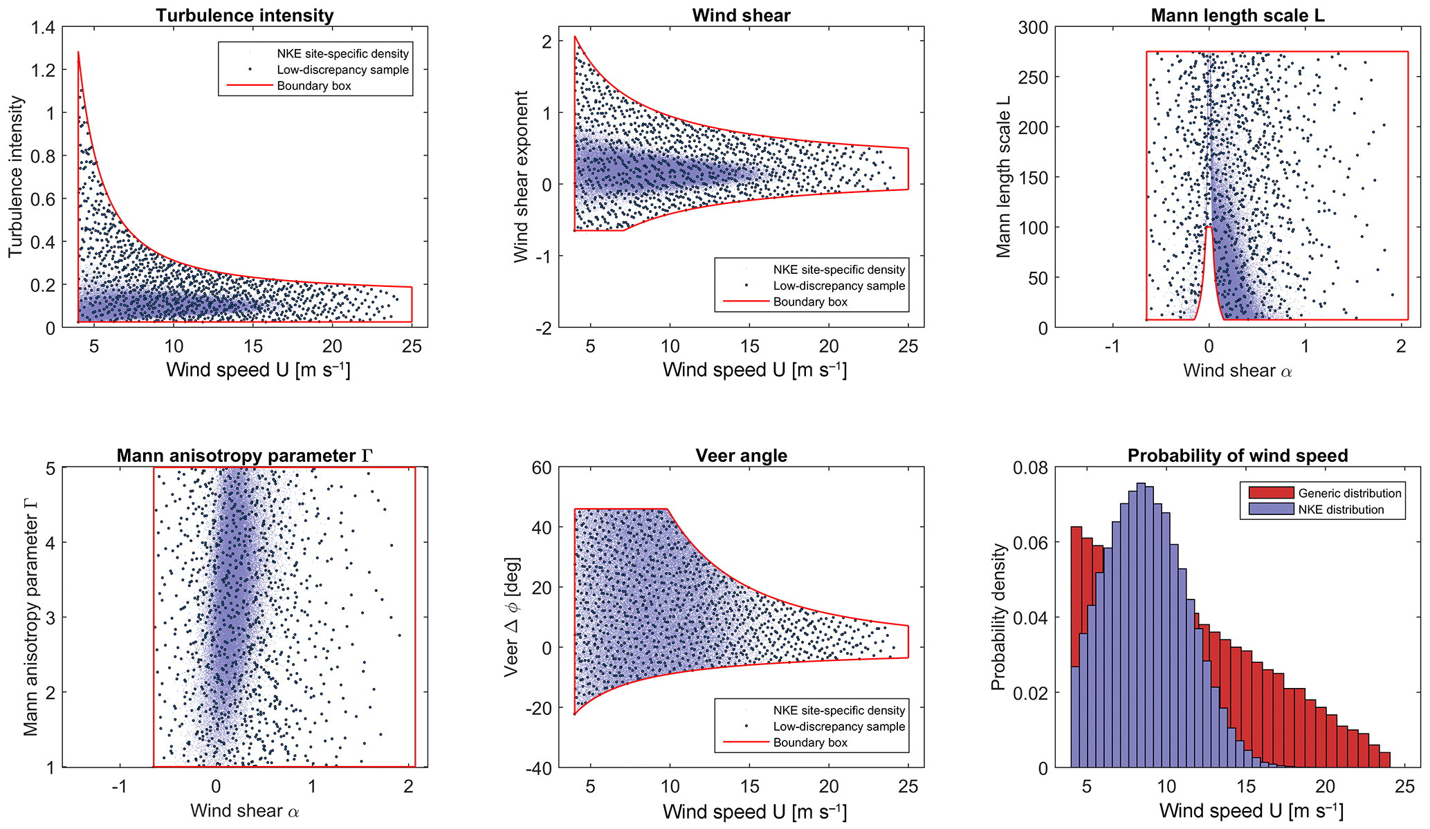
Figure 2Sample distributions obtained using 1024 low-discrepancy points within a 6-dimensional variable space . Here U is beta-distributed, while the other variables are uniformly distributed within their ranges. Solid lines show the sampling space bounds, which are curved due to conditional dependencies. Blue shading shows the site-specific variable distribution for the Nørrekær Enge (NKE) reference site (site 0, cf. Table 5 and Sect. 6.1).
2.4 Sampling procedure
Building a large database with high-fidelity load simulations covering the entire variable space is a central task in the present study as such a database can serve several purposes:
- 1.
be directly used as a site assessment tool by probability weighting the relative contribution of each point to the design loads;
- 2.
serve as an input for calibrating simplified models, i.e., surrogate models and response surfaces.
Characterizing the load behavior of a wind turbine over a range of input conditions requires an experimental design covering the range of variation in all variables with sufficient resolution. In the case of having more than 3–4 dimensions, a full factorial design with multiple levels quickly becomes impractical due to the exponential increase in the number of design points as a function of the number of dimensions. Therefore, in the present study we resort to a MC simulation as the main approach for covering the joint distribution of wind conditions. For assuring better and faster convergence, we use the low-discrepancy Halton sequence in a quasi-MC approach (Caflisch, 1998). While a crude MC integration has a convergence rate proportional to the square root of the number of samples N, i.e., the mean error , the convergence rate for a quasi-MC with a low-discrepancy sequence results in , . For a low number of dimensions and smooth functions, the quasi-MC sequences show a significantly improved performance over the MC sequences, e.g., λ→1; however, for multiple dimensions and discontinuous functions, the advantage over crude MC is reduced (Morokoff and Caflisch, 1995). Nevertheless, even for the full 9-dimensional problem discussed here, it is expected that λ≈0.6 (Morokoff and Caflisch, 1995), which still means about an order of magnitude advantage, e.g., 104 quasi-MC samples should result in about the same error as 105 crude MC samples. A disadvantage of the quasi-random sequences is that their properties typically deteriorate in high-dimensional problems, where periodicity and correlation between points in different dimensions may appear (Morokoff and Caflisch, 1995). However, such behavior typically occurs when more than 20–25 dimensions are used. In the present problem the dimensionality is limited by the computational requirements of the surrogate models and the aeroelastic simulations used to train them. Therefore the behavior of quasi-random sequences in high dimensions does not have implications for the present study. The Halton sequence is applied by consequentially taking all points in the quasi-random series without omission and without repetitions, starting from the second point. The first point in the sequence is discarded as it contains zeros (i.e., the lower bounds of the interval [0,1]) in all dimensions, which corresponds to zero joint probability for the input variables X.
2.5 Database specification
A large-scale generic load database is generated in order to serve as a training data set for the load mapping functions. The point sampling is done using a Halton low-discrepancy sequence within the 9-dimensional variable space defined in Sect. 2.4 (Fig. 2 shows the bounds for the first six variables). The database setup is the following:
-
Up to 104 quasi-random MC sample points in the interval [0,1) are generated, following a low-discrepancy sequence for obtaining evenly distributed points within the parametric space.
-
The physical values of the stochastic variables for all quasi-MC samples are obtained by applying a Rosenblatt transformation using the conditional distribution bounds given in Table 1 and using uniform distribution density, except for the wind speed for which a beta distribution is used.
-
For each sample point, eight simulations, with 3800 s duration each, are carried out. The first 200 s of the simulations are discarded in order to eliminate simulation run-in time transients, and the output is 3600 s (1 h) of load time series from each simulation.
-
The Mann model simulation parameters (L, Γ, αϵ2∕3) that determine the turbulence intensity are tuned to match the required 10 min turbulence statistics (1 h statistics are slightly different due to longer sampling time).
-
Each 1 h time series is split into six 10 min series, which on average will have the required statistics. This leads to a total of 48 10 min time series for each quasi-MC sample point.
-
Simulation conditions are kept stationary over each 1 h simulation period.
-
The DTU 10 MW reference wind turbine model (Bak et al., 2013), with the basic DTU Wind Energy controller (Hansen and Henriksen, 2013), is used in the Hawc2 aeroelastic software (Larsen and Hansen, 2012).
By choosing to run 1 h simulations followed by splitting up of the time series instead of directly simulating 10 min periods, we want to capture some of the low-frequency fluctuations generated by the Mann model turbulence, especially at larger turbulence length scales. When we generate a longer turbulence box, it includes more of these low-frequency variations, which in fact introduce some degree of nonstationarity when looking at 10 min windows.
3.1 Time series postprocessing and cycle counting
The main quantities of interest from the load simulation output are the short-term (10 min) fatigue damage-equivalent loads (DELs), and the 10 min extremes (minimum or maximum, depending on the load type). For each load simulation, four statistics (mean, standard deviation, minimum, and maximum values) are calculated for each load channel. For several selected load channels, the 1 Hz DEL for a reference period Tref are estimated using the expression
where is a reference number of cycles (Nref=600 for obtaining 1 Hz equivalent DEL over a 10 min period), Si are load range cycles estimated using a rain-flow counting algorithm (Rychlik, 1987), and ni are the number of cycles observed in a given range. For a specific material with fatigue properties characterized by an S–N curve of the form (where K is the material-specific Wöhler constant), the fatigue damage D accumulated over one reference period equals
3.2 Definition of lifetime damage-equivalent loads
Obtaining site-specific lifetime fatigue loads from a discrete set of simulations requires integrating the short-term damage contributions over the long-term joint distribution of input conditions. The lifetime damage-equivalent fatigue load is defined as
where f(X) is the joint distribution of the multidimensional vector of input variables X. With the above definition, Seq,lifetime is a function of the expected value of the short-term equivalent loads conditional on the distribution of environmental variables. The integration in Eq. (5) is typically performed numerically over a finite number of realizations drawn from the joint distribution of the input variables, e.g., by setting up a look-up table or carrying out a MC simulation. Thus the continuous problem is transformed into a discrete one:
where , is the ith realization of X out of N total realizations, and p(xi) is the relative, discretized probability of xi, which is derived by weighting the joint pdf values of X so that they satisfy the condition . For a standard MC simulation, each realization is considered to be equally likely, and .
3.3 Uncertainty estimation and confidence intervals
With the present problem of evaluating the uncertainty in aeroelastic simulations – for any specific combination of environmental conditions, xi – there will be uncertainty in the resulting DELs, Seq(xi). Part of this uncertainty is statistical by nature and is caused by realization-to-realization variations in the turbulent wind fields used as input to the load simulations. This uncertainty is normally taken into account by carrying out load simulations with multiple realizations (seeds) of turbulence inputs.
Confidence intervals (CIs) reflecting such an uncertainty can be determined in a straightforward way using the bootstrapping technique (Efron, 1979). Its main advantage is robustness and no necessity for assuming a statistical distribution of the uncertain variable. With this approach, each function realization is given an integer index, e.g., from 1 to N for N function realizations. Then, a “bootstrap” sample is created by generating random integers from 1 to N, and, for each random integer, assigning the original sample point with the corresponding index, as part of the new bootstrap sample. Since the generation of random integers allows for number repetitions, the bootstrap sample will in most cases differ from the original sample. To obtain a measure of the uncertainty in the original sample, a large number of bootstrap samples are drawn, and the resultant quantity of interest (e.g., the lifetime fatigue load) is computed for each of them. Then, the empirical distribution of the set of outcomes is used to define the CIs. If M bootstrap samples have been drawn, and R is the set of outcomes ranked by value in ascending order, then the (CI) bounds for a confidence level cℓ are
where the square brackets [x] indicate the integer part of x, and R[x] means the value in R with rank equal to [x]. In the present study, bootstrapping is applied by generating independent bootstrap samples each with a size equal to the entire data set. Both the sample points and the turbulence seed numbers are shuffled, meaning that the resulting CIs should account for both the statistical uncertainty due to a finite number of samples, and the uncertainty due to seed-to-seed variation. Note that these two uncertainty types are the only ones assumed for the CIs; reducing the CI by creating a large number of model realizations does not eliminate other model uncertainties, nor does it remove uncertainties in the input variables.
In this section we present five different approaches that can be used to map loads from a high-fidelity database to integrated site-specific design loads:
- 1.
importance sampling,
- 2.
nearest-neighbor interpolation,
- 3.
polynomial chaos expansion,
- 4.
universal Kriging, and
- 5.
quadratic response surface.
The first two methodologies carry out a direct numerical integration over the high-fidelity database presented in Sect. 2.5, while the latter three are machine learning models that are trained using the same database. Despite the different nature of the functions, they serve the same purpose and for brevity we will refer to all of them as “surrogate models”.
4.1 Importance sampling
Figure 2 shows the distributions of the first six input variables from our high-fidelity database (Sect. 2.5), along with the site-specific distributions for reference site 0 (see Table 5 for site list).
One of the simplest and most straightforward (but not necessarily most precise) ways of carrying out the integrations needed to obtain predicted statistics is to use importance sampling (IS), where probability weights are applied on each of the database sample points (Ditlevsen and Madsen, 1996). The IS method and various modifications of it are commonly used in wind-energy-related applications (Choe et al., 2015; Graf et al., 2018). In the classical definition of IS, the integration (importance sampling) function for determining the expected value of a function g(X) is given by
where in our application
-
i=1…N is the sample point number;
-
is a 9-component vector array specifying the values of the nine environmental variables considered at sample point i;
-
is the joint pdf of sample point i according to the site-specific probability distribution; and
-
is the joint pdf of sample point i according to the generic probability distribution used to generate the database for the nine variables.
Based on the above, it is clear that only points in the database that also have a high probability of occurrence in the site-specific distribution will have a significant contribution to the lifetime load estimate. This could be considered as a nonstandard application of the IS approach, because typically the IS sample distribution is chosen to maximize the probability density of the integrand. In the present case, this objective can be satisfied only approximately, and only in cases where the number of IS samples is smaller than the total number of database samples (NIS<N). Under these conditions, the importance sampling weights (f(Xi)∕h(Xi) from Eq. 8) can be evaluated for all points in the database. However, the approach adopted in the present paper is to include only the NIS points with the highest weights (as shown in Sect. 6.2).
4.2 Multi-dimensional interpolation
Estimating an expected function value with a true multidimensional interpolation from the high-fidelity database would require finding a set of neighboring points that form a convex polygon. For problem dimensions higher than 3, this is quite challenging due to the nonstructured sample distribution. However, it is much easier to find a more crude approximation by simply finding the database point closest to the function evaluation point in a nearest-neighbor approach. This is similar to the table look-up technique often used with structured grids; the denser the distribution of the sample points is, the closer will the results be to an actual MC simulation. Finding the nearest neighbor to a function evaluation point requires determining the distances between this point and the rest of the points in the sample space. This is done most consistently in a normalized space, i.e., where the input variables have equal scaling. The cumulative distribution function (CDF) of the variables is an example of such a space, as all CDFs have the same range of (0,1). Thus, the normalized distance between a new evaluation point and an existing sample is computed as the vector norm of the (e.g., 9-dimensional vector) differences between the marginal CDF for the two points:
where is the difference between the current evaluation point Y and the existing sample points in the reference database, . The vector consists of the marginal CDFs of the input variables X as obtained using a Rosenblatt transformation.
Since some of the input variables may have significantly bigger influence on the result than other variables, it may be useful to weight the CDF of different variables according to their importance (e.g., by making the weights proportional to the variable sensitivity indices; see Sect. 4.6).
4.3 Polynomial chaos expansion
Polynomial chaos expansion (PCE) is a popular method for approximating a stochastic function of multiple random variables using an orthogonal polynomial basis. For the present problem, using a Wiener–Askey generalized PCE (Xiu and Karniadakis, 2002) employing Legendre polynomials is considered most suitable for any (scaled) variable . Because Legendre polynomials Pn(ξ) are orthogonal with respect to a uniform probability measure, the PCE can conveniently be applied to the CDFs of the variables X that are defined in the interval [0,1]. Then
where F(Xi) is the cumulative distribution function of a variable Xi∈X, . The Legendre polynomial coefficients can be generated using the recurrence relation
where the first two entries, P0(ξ)=1 and P1(ξ)=ξ, serve for initialization. The aim of using PCE is to represent a scalar quantity S=g(X) in terms of a truncated sequence , where ε is a zero-mean residual term. With this definition, the multivariate generalized PCE of dimension M and maximum degree p is given by
here Ψγ are multivariate orthogonal polynomials composed of the product of univariate polynomials having (nonnegative integer) orders defined by the vector , with the total of orders being constrained by the degree: . The unknown coefficients need to be determined, and are functions of X as defined in Eq. (10). Training the PCE model amounts to determining the vector of coefficients, S. For a more detailed explanation of the training process, as well as the basic PCE theory, the reader is referred to Appendix A (Sudret, 2008; Xiu and Karniadakis, 2002).
4.4 Universal Kriging with polynomial chaos basis functions
Kriging (Sacks et al., 1989; Santher et al., 2003) is a stochastic interpolation technique that assumes the interpolated variable follows a Gaussian process. A Kriging model is described (Sacks et al., 1989) by
where for N evaluation samples and an M-dimensional problem, X represents an M×N matrix of input variables and Y(X) is the output vector. The term f(X)Tβ is the mean value of the Gaussian process (a.k.a. the “trend”) represented as a set of basis functions and regression coefficients , whereas Z(X) is a zero-mean stationary Gaussian process. The (joint) probability distribution of the Gaussian process is characterized by its covariance; for two distinct “points” X and W in the sample domain the covariance is defined as
where σ2 is the overall process variance that is assumed to be constant, and is the correlation between Z(X) and Z(W). The hyperparameters θ define the correlation behavior, in terms of correlation length scale(s) for example. Since the mean and variance of the Gaussian field can be expressed as functions of θ (this is shown in details in Appendix A), the calibration of the Kriging model amounts to determining the trend coefficients and obtaining an optimal solution for θ.
The functional form of the mean field f(X)Tβ is identical to the generalized PCE defined in Eq. (27), meaning that the PCE is a possible candidate model for the mean in a Kriging interpolation. We adopt this approach and define the Kriging mean as a PCE with properties as described in Sect. 4.3. A suitable approach for tuning the Gaussian field statistics is to find the values of β, σ2 and θ that maximize the likelihood of the training set variables Y, i.e., minimize the model error in a least-squares sense (Lataniotis et al., 2015). This is described in Appendix A.
The main practical difference between regression- or expansion-type models such as regular PCE and the Kriging approach is how the training sample is used in the model: in pure regression-based approaches the training sample is used to only calibrate the regression coefficients, while in Kriging (and in other interpolation techniques) the training sample is retained and used in every new model evaluation. As a result the Kriging model may have an advantage in accuracy, since the model error tends to zero in the vicinity of the training points; however, this comes at the expense of an increase in the computational demands for new model evaluations. For a Kriging model, a gain in accuracy over the model represented by the trend function will only materialize in problems where there is a noticeable correlation between the residual values at different training points. In a situation where the model error is independent from point to point (e.g., in the case when the error is only due to seed-to-seed variations in turbulence) the inferred correlation length will tend to zero and the Kriging estimator will be represented by the trend function alone.
4.5 Quadratic response surface
A quadratic-polynomial response surface (RS) method based on central composite design (CCD) is a reduced-order model which, among other applications, has been used for wind turbine load prediction (Toft et al., 2016). The procedure involves fitting a quadratic polynomial regression (“response surface”) to a normalized space of i.i.d. variables, which are derived from the physical variables using an isoprobabilistic transformation – such as the Rosenblatt transformation given in Eqs. (1) and (2). The design points used for calibrating the response surface in k dimensions form a combination of a central point, axial points a distance of in each dimension, and a 2k “factorial design” set where there are two levels (points) per variable dimension located at unit distance from the origin; this is shown in Fig. 3 for the case of k=2 variables (dimensions). Due to the structured design grid required, it is not possible to use this approach with the sample points from the high-fidelity database described in Sect. 2; therefore, we implement the procedure using an additional set of simulations. The low order of the response surface also prohibits full characterization of the highly nonlinear turbine response as a function of mean wind speed using a single response surface. Therefore, multiple response surfaces are calibrated for wind speeds from 4 to 25 m s−1 in 1 m s−1 steps. This approach may in principle be extended to include additional variables such as turbulence (σu), but doing so will reduce the practicality of the procedure as it will require multidimensional interpolation between a large number of models and the uncertainty may increase. However, due to the exponential increase in the number of design points with increasing problem dimension, it is not practical to fit a response surface covering all nine variables considered. Instead, we choose to replace three of the variables with relatively low importance (yaw, tilt, and air density) with their mean values. The result is a 6-dimensional problem consisting of 22 different 5-dimensional response surfaces, which require design points in total. Analogous to the high-fidelity database, 8 h of simulations are carried out for characterizing each design point. The polynomial coefficients of the response surface are then defined using least-squares regression with the same closed-form solution defined by Eq. (27). For any sample point p in the CCD, the corresponding row in the design matrix is defined as
where U are standard normal variables derived from the physical variables X by an isoprobabilistic transformation.
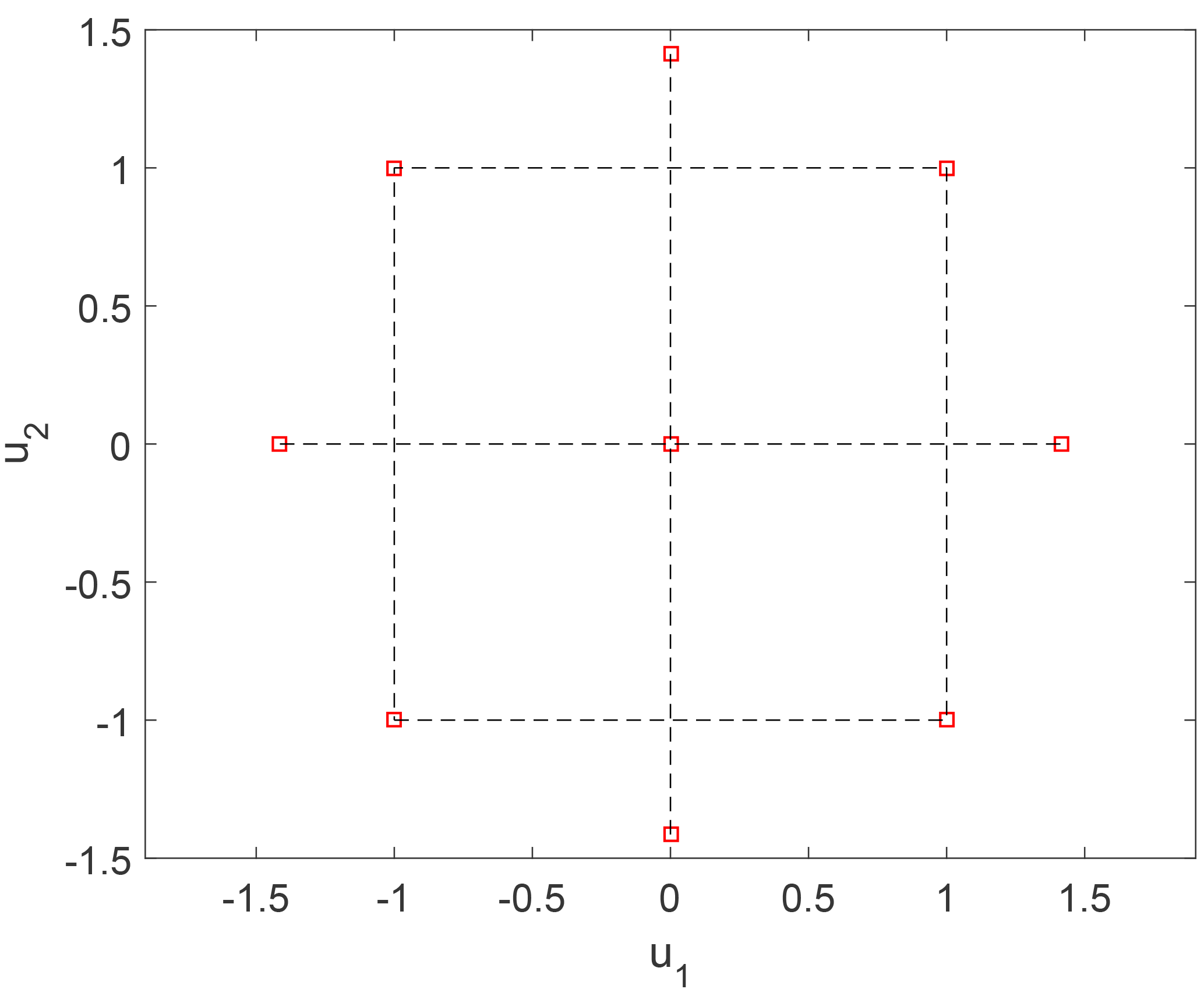
Figure 3Example of a rotatable central composite design (CCD) in a 2-dimensional standard normal space [u1,u2]. The CCD consists of a central point, a 2k “factorial design” with 2 levels and k=2 dimensions, and axial points at distance , meaning that all the outer points lie on a circle.
4.6 Sensitivity indices
We use the global Sobol indices, Sobol (2001), for evaluating the sensitivity of the response with respect to input variables. Having trained a surrogate model, the total Sobol indices can be computed efficiently by carrying out a MC simulation on the surrogate. For number of dimensions equal to M (e.g., M=9 in the present study) and for N (quasi) MC samples the required experimental design represents an N×2M matrix. This is divided into two N×M matrices, A and B. Then, for each dimension i, i=1…M, a third matrix ABi is created by taking the ith column of ABi equal to the ith column from B, and all other columns taken from A. The load surrogate is then evaluated for all three matrices, resulting in three model estimates: f(A), f(B), and f(ABi). By repeating this for i=1…M, simulation-based Sobol' sensitivity indices can be estimated as
where j=1…N is the row index in the design matrices A, B, and ABi (Saltelli et al., 2008). For the problem discussed in the present study, it was sufficient to use approximately 500 MC samples per variable dimension in order to compute the total Sobol indices.
4.7 Model reduction
For any polynomial-based regression model that includes dependence between variables, the problem grows steeply in size when the number of dimensions, M, and the maximum polynomial order, p, increase. In such situations, it may be desirable to limit the number of active coefficients by carrying out a least absolute shrinkage and selection operator (LASSO) regression (Tibshirani, 1996), which regularizes the regression by penalizing the sum of the absolute value of regression coefficients. For a PCE model, the objective function using a LASSO regularization is
where λ is a positive regularization parameter; larger values of λ increase the penalty and reduce the absolute sum of the regression coefficients, while λ=0 is equivalent to ordinary least-squares regression. In the present study, the LASSO regularization is used on the PCE-based models to reduce the number of coefficients.
One useful corollary of the orthogonality in the PCE polynomial basis is that the contribution of each individual term to the total variance of the expansion (i.e., the individual Sobol indices) can be easily computed based on the coefficient values (see Appendix A). This property can be used for eliminating polynomials that do not significantly contribute to the variance of the output, thus achieving a sparse, more computationally efficient, reduced model. By combining the variance truncation and the LASSO regression technique in Eq. (17), a model reduction of an order of magnitude or more can be achieved. For example, for the 9-dimensional PCE of order 6 discussed in Sect. 5.3, using LASSO regularization parameter λ=1 and retaining the polynomials that have a total variance contribution of 99.5 % resulted in a reduction of the number of polynomials from 5005 to about 200.
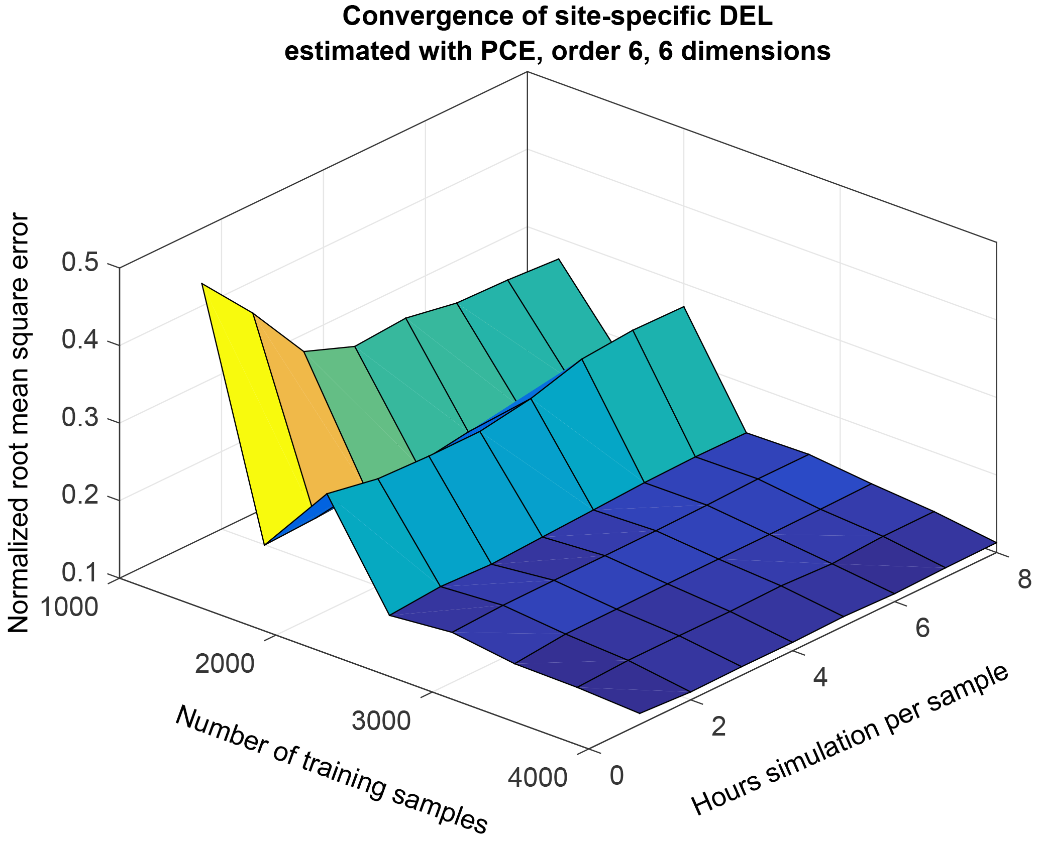
Figure 4Convergence of a PCE of dimension 6 and order 6, as a function of number of collocation points and hours of simulation per collocation point. The z axis represents the NRMSE obtained from the difference between 500 site-specific quasi-MC samples of blade root flapwise DEL for reference site 0, and the corresponding predictions from PCE.
5.1 Model convergence
We assess the convergence of PCE by calculating the normalized root-mean-square error (NRMSE) between a set of observed quantities (i.e., DELs from simulations) , and the PCE predictions, , over the same set of N sample points X(i) from the training sample defined in Sect. 2:
where E[y] is the expected value of the observed variable. Figure 4 shows the NRMSE for a non-truncated PCE of order 6 and with six dimensions as a function of the number of samples used to train the PCE, and the hours of load simulations (i.e., number of seeds) used for each sample point. The NRMSE shown in Fig. 4 is calculated based on a set of 500 quasi-MC points sampled from the joint pdf of reference site 0, and represents the difference in blade root flapwise DEL observed in each of the 500 points vs. the DEL predicted by a PC expansion trained on a selection of points from the high-fidelity database described in Sect. 2. Each of the quasi-MC samples is the mean from 48 turbulent 10 min simulations. To mimic the seed-to-seed uncertainty, each of the PCE predictions is also evaluated as the mean of 48 normally distributed random realizations, with mean and standard deviation prescribed by the PCE model for mean and standard deviation of the blade flapwise DEL, respectively.
Figure 4 illustrates a general tendency that using a few thousand training samples leads to convergence of the values of the PC coefficients, and the remaining uncertainty is due to seed-to-seed variations and due to the order of the PCE being lower than what is required for providing an exact solution at each sample point. Using longer simulations per sample point does not lead to further reduction in the statistical uncertainty due to seed-to-seed variations – with 4000 training samples, the NRMSE for 1 h simulation per sample is almost identical to the error with 8 h simulation per sample. The explanation for this observation is that the seed-to-seed variation introduces an uncertainty not only between different simulations within the same sampling point but also between different sampling points. This uncertainty materializes as an additional variance which is not explained by the smooth PCE surface. Further increase in the number of training points or simulation length will only reduce this statistical uncertainty, but will not contribute significantly to changes in the model predictions as the flexibility of the model is limited by the maximum polynomial order. Therefore, the model performance achieved under these conditions can be considered near to the best possible for the given PCE order and number of dimensions. However, it should be noted that the number of training points required for such convergence will differ according to the order and dimension of the PCE, and higher order and more dimensions will require more than the approximately 3000 points that seem sufficient for a PCE of order 6 with six dimensions, as shown in Fig. 4.
The IS procedure has relatively slow convergence compared to, for example, a quasi-MC simulation. Figure 5 shows an example of the convergence of an IS integration for reference site 0, based on computing the target (site-specific) distribution weights for all 104 points in a reference high-fidelity database. The CIs are obtained by bootstrapping.
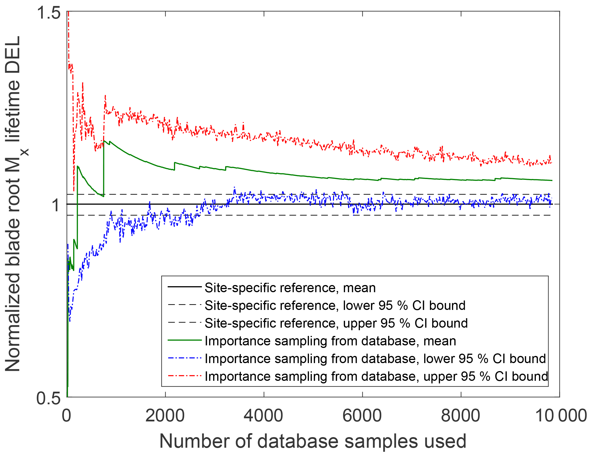
Figure 5Convergence of an importance sampling (IS) calculation of the blade root moment from the high-fidelity database towards site-specific lifetime fatigue loads for reference site 0 (Table 5).
Table 2Normalized root mean square error characterizing the difference between aeroelastic simulations and reduced-order models. Load channel abbreviations are the following: TB: tower base; TT: tower top; MS: main shaft; BR: blade root. Loading directions consist of Mx: fore-aft (flapwise) bending, My: side-side (edgewise) bending, and Mz: torsion.
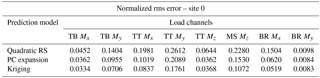
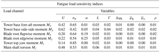
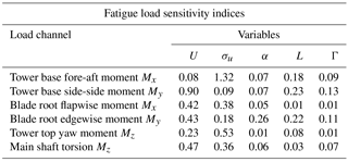
Table 3PCE-based Sobol sensitivity indices for the high-fidelity load database variable ranges.
5.2 One-to-one comparison and mean squared error
Since the prediction of lifetime fatigue loads is the main purpose of the present study, the performance of the load prediction methods with respect to estimating the lifetime DEL is the main criterion for evaluation. However, the lifetime DEL as an integrated quantity will efficiently identify model bias but may not reveal the magnitude of some uncertainties that result in zero-mean error. As an additional means of comparison we calculate the NRMSE, defined in Eq. (18), resulting from a point-by-point comparison of load predictions from a reduced-order model against actual reference values. The reference values are the results from the site-specific aeroelastic load simulations for reference site 0. At each sample point, the reference value yi represents the mean DEL from all turbulence seeds simulated with these conditions. The values of the NRMSE for site 0 for Kriging, RS, and PCE-based load predictions are listed in Table 2. In addition, Fig. 6 presents a one-to-one comparison where for a set of 200 sample points, the load estimates from the site-specific MC simulations are compared against the corresponding surrogate model predictions in terms of y−y plots.
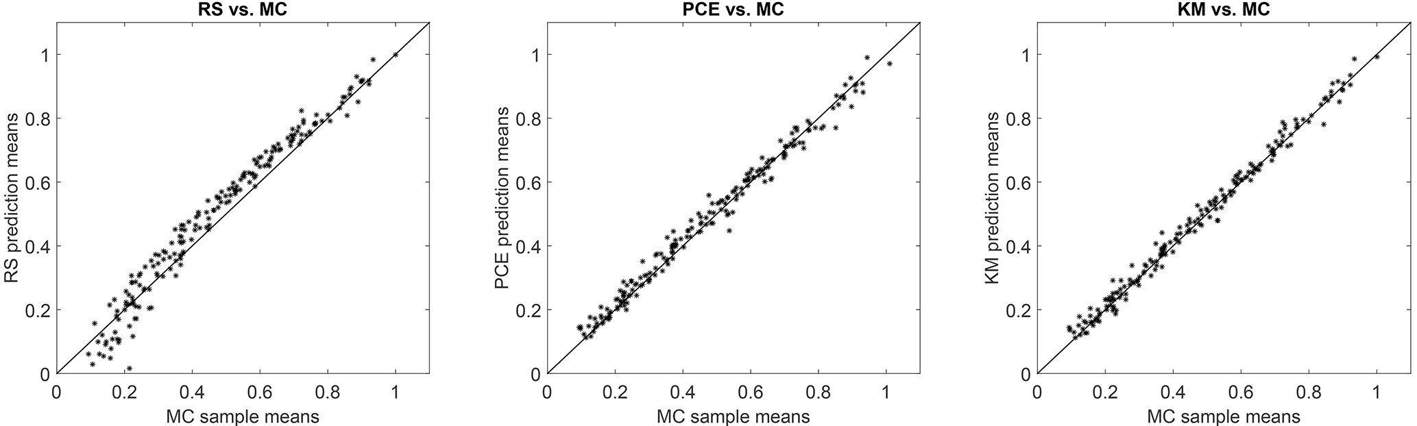
Figure 6y−y plots comparing the blade root flapwise 1 Hz damage-equivalent load (DEL) predictions for three load surrogate models – quadratic Response Surface, Polynomial Chaos expansion, and Kriging model, compared against site-specific Monte Carlo (MC) simulation. The x axis represents the loads obtained using site-specific MC simulations for reference site 0, and the y axis represents the mean 1 Hz-equivalent load estimated for the same sample points using a surrogate model. All values are normalized with the maximum equivalent load attained from the site-specific Monte Carlo (MC) simulation.
The RMS error analysis reveals a slightly different picture. In contrast to the lifetime DEL where the Kriging, PCE, and RS methods showed very similar results, the RMS error of the quadratic RS is for some channels about twice the RMS error of the other two approaches.
5.3 Variable sensitivities
As described earlier in Sect. 4.6, we consider variable sensitivities (i.e., the influence of input variables on the variance of the outcome) in terms of Sobol indices. By definition the Sobol indices will be dependent on the variance of input variables, meaning that for one and the same model, the Sobol indices will be varying under different (site-specific) input variable distributions. Taking this into account, we evaluate the Sobol indices for the two types of joint variable distributions used in this study – (1) a site-specific distribution, and (2) the joint distribution used to generate the database with high-fidelity load simulations. The total Sobol indices for the high-fidelity load database variable range are computed directly from the PCE fitted to the database by evaluating the variance contributions from the expansion coefficients (see Appendix A) and are listed in Table 3. The indices for the site-specific distribution corresponding to reference site 0 are computed using the method based on MC simulations described in Sect. 4.6, as direct PCE indices are not available for this sample distribution. The resulting total Sobol indices for the six variables available at site 0 are listed in Table 4. The two tables show similar results – the mean wind speed and the turbulence are the most important factors affecting both fatigue and extreme loads. Two other variables that show a smaller but still noticeable influence are the wind shear, α, and the Mann model turbulence length scale, L. The effect of wind shear is pronounced mainly for blade root loads that can be explained by the rotation of the blades, which, if subjected to wind shear, will experience cyclic changes in wind velocity. The effect of Mann model Γ, veer, yaw, tilt, and air density within the chosen variable ranges seems to be minimal, especially for fatigue loads.
Table 4Site-specific Sobol sensitivity indices derived for site 0 using MC simulation from a PCE.
6.1 Reference sites
The low-fidelity site-specific load calculation methods presented in this study are validated against a set of reference site-specific load calculations on a number of different virtual sites, based on real-world measurement data that cover most of the variable domain included within the high-fidelity database. In order to show a realistic example of situations where a site-specific load estimation is necessary, the majority of the virtual sites chosen are characterized with conditions that slightly exceed the standard conditions specified by a certain type-certification class. Exceptions are site 0, which has the most measured variables available and is therefore chosen as a primary reference site, and the virtual “sites” representing standard IEC class conditions. The IEC classes are included as test sites as they are described by only one independent variable (mean wind speed). They are useful test conditions as it may be challenging to correctly predict loads as a function of only one variable using a model based on up to nine random variables. The list of test sites is given in Table 5.
Table 5Reference virtual sites used for validation of the site-specific load estimation methods.
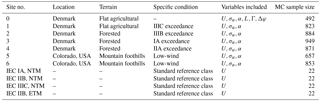
Site 0 (also referred to as the reference site) is located at the Nørrekær Enge wind farm in northern Denmark (Borraccino et al., 2017), over flat, open agricultural terrain. Site 1 is a flat-terrain near-coastal site at the National Centre for Wind Turbines at Høvsøre, Denmark (Peña et al., 2016). Sites 2 to 4 are based on the wind conditions measured at the Østerild Wind Turbine Test Field, which is located in a large forest plantation in northwestern Denmark (Hansen et al., 2014). Due to the forested surroundings of the site, the flow conditions are more complex than those in Nørrekær Enge and Høvsøre. By applying different filtering according to wind direction, three virtual site climates are generated and considered as sites 2–4.
Sites 5 and 6 are located at NREL's National Wind Technology Center (NWTC), near the base of the Rocky Mountain foothills just south of Boulder, Colorado (Clifton et al., 2013). Similar to Østerild, directional filtering is applied to the NTWC data to split it into two virtual sites – accounting for the different conditions and wind climates from the two ranges of directions considered.
For each site, the joint distributions of all variables are defined in terms of conditional dependencies, and generating simulations of site-specific conditions is carried out using the Rosenblatt transformation, Eq. (1). The conditional dependencies are described in terms of functional relationships between the governing variable and the distribution parameters of the dependent variable, e.g., the mean and standard deviation of the turbulence are modeled as linearly dependent on the wind speed as recommended by the IEC 61400-1 (ed. 3, 2005) standard. The wind shear exponent is dependent on the mean wind speed and on the turbulence, and the distribution parameters of α are defined by the relationship (Dimitrov et al., 2015; Kelly et al., 2014)
where μα and σα are the mean and standard deviation of α, respectively; is a characteristic turbulence intensity based on a turbulence quantile Q, as a function of the wind speed U. Here m s−1) is the reference characteristic turbulence intensity at U=15m s−1 and m s−1) is a reference wind shear exponent, with αc being an empirically determined constant. Since the turbulence quantities Ic(u) and Ic,ref are defined by the conditional relationship between wind speed and turbulence, the only site-specific parameters required for characterizing the wind shear are αref and cα. For each of the physical sites, the wind speed, turbulence and wind shear distribution parameters are defined based on anemometer measurements at the sites. The results are listed in Table 6. In addition, high-frequency 3-D sonic measurements were available at site 0 for the entire measurement period, which allowed for estimating Mann turbulence model parameters using the approach described in Dimitrov et al. (2017).
With this procedure, 1000 quasi-MC samples of the environmental conditions at each site are generated from the respective joint distribution. All realizations where the wind speed is between the DTU 10 MW wind turbine cut-in and cut-out wind speed are fed as input to load simulations. The actual number of load simulations for each site are given in Table 6. Similarly to the load database simulations, eight simulations with 1 h duration are carried out at each site-specific MC sample point. The resulting reference lifetime equivalent loads are then defined by applying Eq. (6) on the MC simulations using equal weights , while the uncertainty in the lifetime loads is estimated using bootstrapping on the entire MC sample.
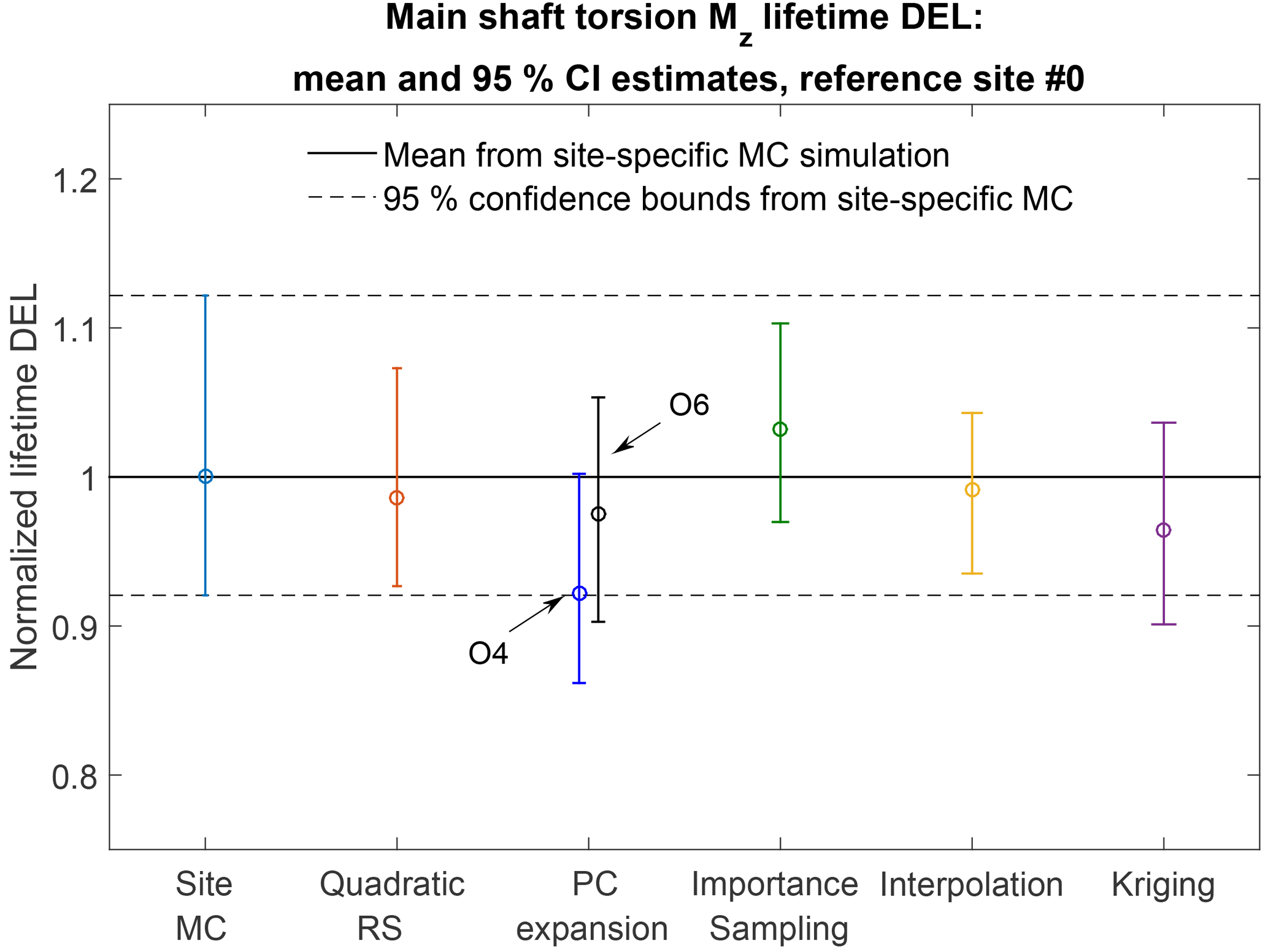
Figure 7Comparison of predictions of the lifetime damage-equivalent loads (DELs) for six different estimation approaches. All values are normalized with respect to the mean estimate from a site-specific Monte Carlo (MC) simulation, and the error bars represent the bounds of the 95 % confidence intervals (CIs). Results from two PCEs are shown: the blue bar corresponds to the output of a fourth-order PCE, while the black bar corresponds to a sixth-order PCE.
Table 6Parameters defining the conditional distribution relationships used in computing joint distributions of the environmental conditions for the test sites/conditions.
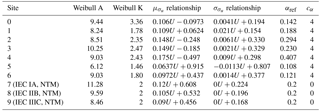
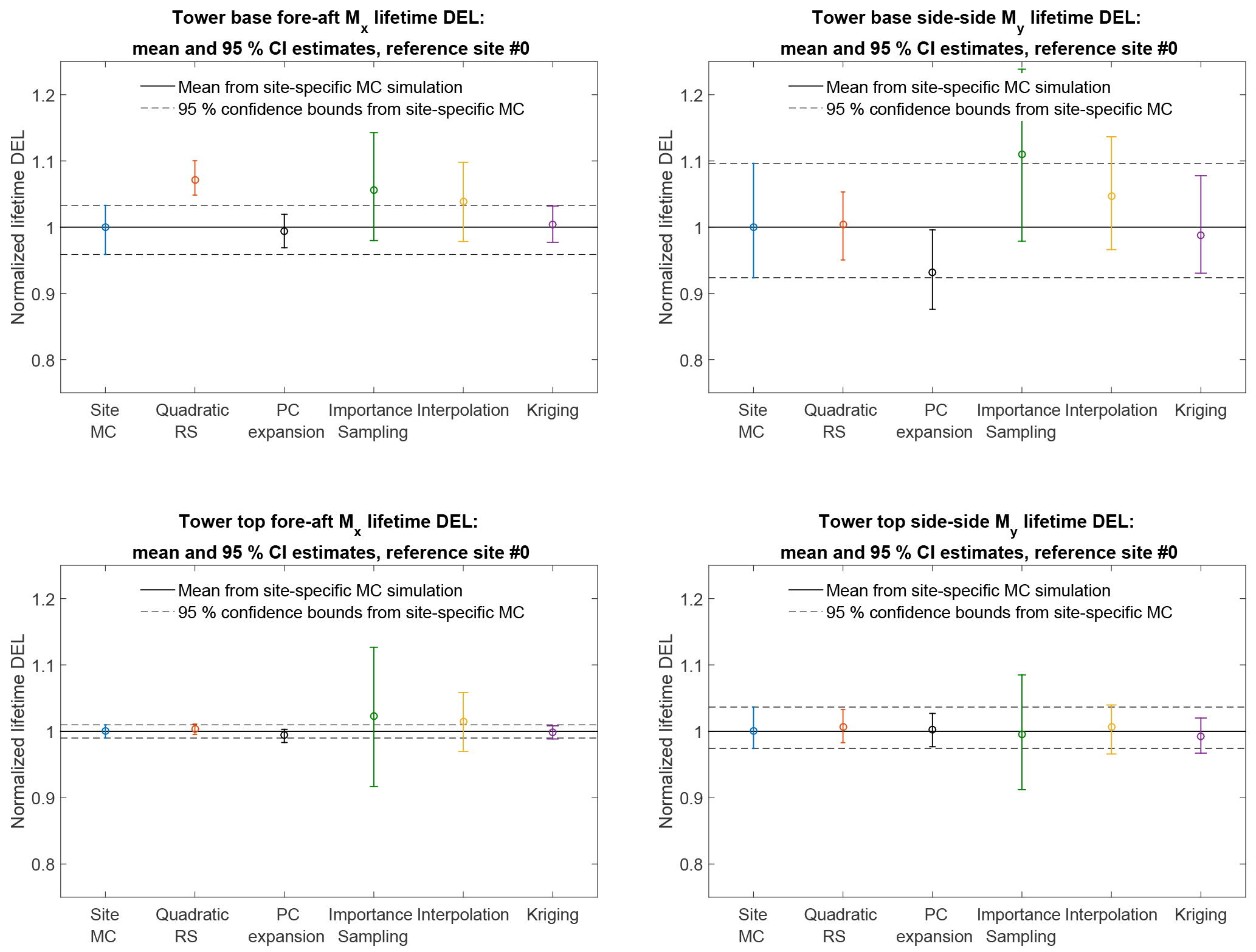
Figure 8Comparison of predictions of the lifetime damage-equivalent loads (DELs) for six different estimation approaches. All values are normalized with respect to the mean estimate from a site-specific Monte Carlo simulation.
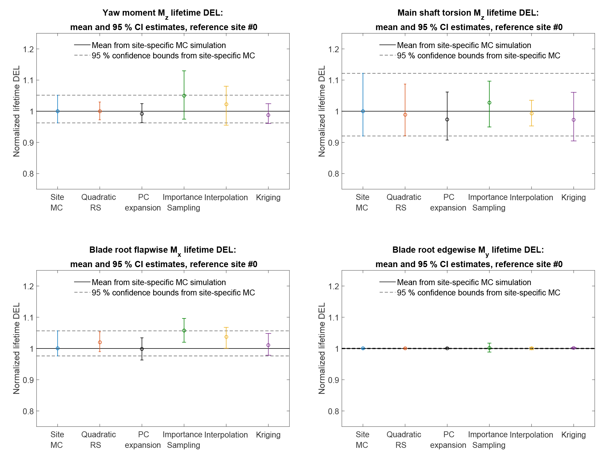
Figure 9Comparison of predictions of the lifetime damage-equivalent loads (DELs) for six different estimation approaches. All values are normalized with respect to the mean estimate from a site-specific Monte Carlo simulation.
6.2 Lifetime fatigue loads
The lifetime damage-equivalent loads (DELs) are computed for all reference sites in Table 5, using the five load surrogate models defined above: (1) quadratic response surface; (2) polynomial chaos expansion, (3) importance sampling, (4) nearest-neighbor interpolation, and (5) Kriging with the mean defined by polynomial chaos basis functions. Methods 2–5 are based on data from the high-fidelity load database described in Sect. 2. In addition to the surrogate model computations, a full MC reference simulation is carried out for each validation site. The load predictions with the MC approach are obtained by carrying out Hawc2 aeroelastic simulations on the same DTU 10 MW reference wind turbine model used for training the load surrogate models. A total of NMC=1000 quasi-MC samples are drawn from the joint distribution of environmental input variables characterizing each site, and 8 h of aeroelastic simulations are carried out for each of the quasi-MC samples where the wind speed is between cut-in and cut-out. An exception is the IEC-based sites, where the standard IEC procedure is followed and loads are evaluated for 22 wind speeds from cut-in to cut-out in 1 m s−1 steps. For each site, the full MC simulation is then used as a reference to test the performance of the other five methods. The load predictions from the PCE, Kriging, quadratic RS, and the nearest-neighbor interpolation procedures all use a quasi-MC simulation of the respective model with the same sample set of environmental inputs used in the reference MC simulations. The load predictions with importance sampling are based on the probability-weighted contributions from the samples in a high-fidelity load database. For each site-specific distribution, the database samples are ordered according to their weights, and only a number of points, NIS, with the highest weights are used in the estimation. For the sake of easier comparison between different methods, it is chosen that NIS=NMC. Based on computations from PCE with a different number of dimensions and different maximum order, it was observed that expansions of order 4 or 5 may not be sufficiently accurate for some response channels. This is illustrated in Fig. 7 where the prediction of main shaft torsion loads using order 4 and order 6 PC expansion are compared against other methods, and the order 4 calculation shows a significant bias. Therefore, the PC expansion used for reporting the results in this section is based on the same 6-dimensional variable input used with the quadratic response surface, and has a maximum order of 6. For evaluating CIs from the reduced-order models (Kriging, PCE, and quadratic response surface), two reduced-order models of each type are calibrated – one for the mean values, and the other for the standard deviations. This allows for generating a number of realizations for each sampled combination of input variables, and subsequently computing CIs by bootstrapping (Eq. 7). In this way, the bootstrapping is done simultaneously for a random sample of the input variables and the random seed-to-seed variations within each sample. As a result, the obtained CI reflects the combination of seed-to-seed uncertainty and the uncertainty due to a finite number of samples from the distribution of the input variables. This approach also allows for consistency with the importance sampling and nearest-neighbor interpolation techniques, where the same bootstrapping approach is used. Since the lifetime fatigue load is in essence an integrated quantity subject to the law of large numbers, the uncertainty in computations based on a random sample of size N will be proportional to . Comparing uncertainties and CIs as defined in Sect. 3.3 will therefore only be meaningful when approximately the same number of samples is used for all calculation methods. This approach is used for generating Figs. 8 and 9, where the performance of all site-specific load estimation methods is compared for reference site 0, for eight load channels in total, with the number of samples as listed in Table 8. Figure 8 shows results for tower base and tower top fore-aft and side-side bending moments, and Fig. 9 displays the tower top yaw moment, the main shaft torsion, and blade root flapwise and edgewise bending moments.
Table 7Lifetime-equivalent load predictions normalized with respect to MC simulations and averaged over 10 reference sites. Load channel abbreviations are the following: TB: tower base; TT: tower top; MS: main shaft; BR: blade root. Loading directions consist of Mx: fore-aft (flapwise) bending; My: side-side (edgewise) bending; and Mz: torsion.
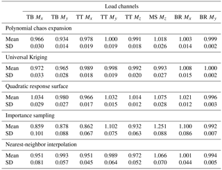
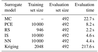
Table 8Model execution times for the lifetime damage-equivalent fatigue load computations for site 0.
The results for site 0 show that for all methods the prediction of blade root and tower top loads is more accurate than the prediction of tower base loads. Also, overall the predictions from the reduced models – the quadratic RS and the PCE, as well as from the Kriging model – are more robust than the IS and nearest-neighbor (NN) interpolation techniques. Similar performance is observed for most other validation sites. The summarized site-specific results for all surrogate-based load estimation methods are shown in Table 7. In order to compute these values, the load estimates for each site and load channel are normalized to the results obtained with the direct site-specific MC simulations. The values given in Table 7 are averaged over all reference sites. The results for individual sites and load channels are depicted as bar plots in Figs. 10 and 11 for tower load and rotor load channels, respectively. The largest observed errors amount to ≈9 % with Kriging, ≈10 % for the PCE, ≈10 % for the quadratic RS, ≈24 % for IS, and ∼15–17 % for NN interpolation. Noticeably, the low wind speed, high turbulence site 5 seems to be the most difficult for prediction – for most load prediction methods this is the site where the largest error is found. All models except the Kriging also show relatively large errors for the IEC class-based sites. That can be attributed to the significantly smaller number of samples used for the IEC-based sites (22 samples where only the wind speed is varied in 1 m s−1 steps from 4 to 25 m s−1). As mentioned above, the statistical uncertainty in the estimation of the lifetime DEL will diminish with increasing number of samples. In addition to this effect, as discussed in Sect. 4.1, the uncertainty in the IS model can increase when the site-specific distribution has fewer dimensions than the model because fewer points from the high-fidelity database will have high probabilities with respect to the site-specific distribution. It can be expected that this effect is strongest for the IEC class-based sites, as for them only a single variable – the wind speed – is considered stochastic.
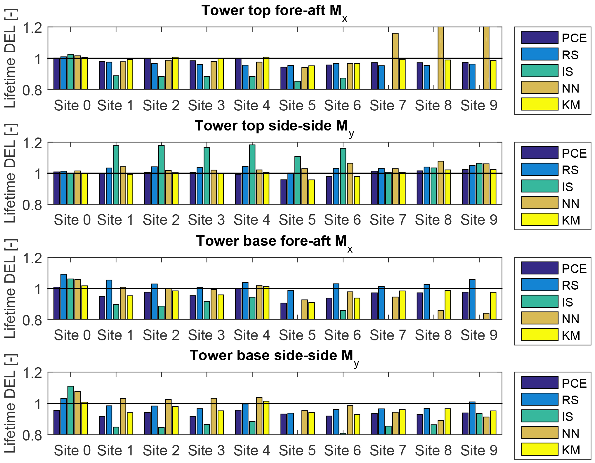
Figure 10Predictions of lifetime damage-equivalent tower loads for five different estimation approaches and four load channels for the different sites (0–6) and IEC conditions (virtual sites 7–9). All values are normalized with respect to the mean estimate from a site-specific Monte Carlo (MC) simulation. The abbreviations refer to PCE: polynomial chaos expansion; RS: quadratic response surface; IS: importance sampling; NN: nearest-neighbor interpolation; and KM: universal Kriging model.
Another important aspect to consider when comparing the performance of the surrogate models is the model execution speed, and whether there is a tradeoff between speed and accuracy. A comparison of the model evaluation times for the site-specific lifetime load computation for site 0 is given in Table 8. Noticeably, the Kriging model requires significantly longer execution time than other approaches, which is mainly due to the requirement of populating a cross-correlation matrix.
7.1 Discussion
The previous sections of this paper described a procedure for estimating site-specific lifetime damage-equivalent loads (DELs), using several simplified model techniques applied to 10 different sites and conditions. Based on the site-specific lifetime DEL comparisons, for quick site-specific load estimation, the three models based on machine learning were most viable (sufficiently accurate over the majority of the sampling space): polynomial chaos expansion, Kriging, and the quadratic response surface (RS). When estimating lifetime DEL, these methods showed approximately equal levels of uncertainty. However, in the one-to-one comparisons, the quadratic RS model showed larger error, especially for sample points corresponding to more extreme combinations of environmental conditions. This is due to the lower order and the relatively small number of calibration points of the quadratic RS, which means that the model accuracy decreases in the sampling space away from the calibration points, especially if there is any extrapolation. This inaccuracy is reflected in the NRMSE from one-to-one comparisons, but is less obvious in the lifetime fatigue load computations that average out errors with zero mean. The universal Kriging model demonstrated the smallest overall uncertainty, both in sample-to-sample comparisons and in lifetime DEL computations. This is to be expected since the Kriging employs a well-performing model (the PCE) and combines it with an interpolation scheme that subsequently reduces the uncertainty even further. However, in most cases the observed improvement over a pure PCE is not significant. This indicates that the sources of the remaining uncertainty are outside the models – e.g., the seed-to-seed turbulence variations: the models being calibrated with turbulence realizations different from the ones used to compute the reference site-specific loads. As a result, the trend function (the β term in Eq. 13) is the primary contribution to the Kriging estimator, and the influence of the Gaussian-field interpolation is minimal. A drawback of the Kriging model with respect to the other techniques is the larger computational demands due to the need of computing correlation matrices and the use of the training sample for each new evaluation.
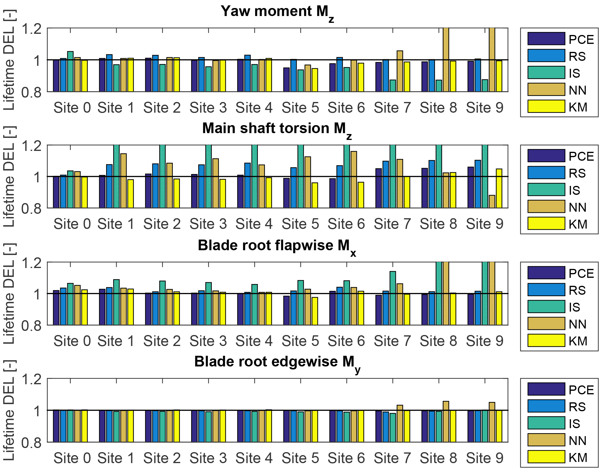
Figure 11Predictions of lifetime damage-equivalent loads (yaw, shaft torsion, blade-root) for five different estimation approaches and four load channels. All values are normalized with respect to the mean estimate from a site-specific Monte Carlo (MC) simulation. The abbreviations refer to PCE: polynomial chaos expansion; RS: quadratic response surface; IS: importance sampling; NN: nearest-neighbor interpolation; and KM: universal Kriging model.
For all site-specific load assessment methods discussed, the estimations are trustworthy only within the bounds of the variable space used for model calibration – extrapolation is either not possible or may lead to unpredictable results. It is therefore important to ensure that the site-specific distributions used for load assessment are not outside the bounds of validity of the load estimation model.
The variable bounds presented in this paper are based on a certain degree of consideration of atmospheric physics employed in the relationships between wind speed, turbulence, wind shear, wind veer, and turbulence length scale. The primary scope is to encompass the ranges of conditions relevant for fatigue load analysis, and the currently suggested variable bounds include all normal-turbulence (NTM) classes. However, for some other calculations it may be more practical to choose other bound definitions; for example, for the extreme turbulence models prescribed by the IEC 61400-1, the currently suggested bounds do not include ETM class A.
For the more advanced methods like PCE and Kriging, there is a practical limitation on the number of training points to be used in a single-computer setup. For a PCE the practical limit is mainly subject to memory availability when assembling and inverting the information matrix, and for a PCE of order 6 and with nine dimensions, this limit is on the order of 1–2×10⁴ points on a typical desktop computer (as of 2018). For Kriging, the computing time also plays a role: although a similar number of training points could be stored in memory as for the PCE, the computational time is much longer, and the practical limit of training points for most applications is less than for the PCE. However, as it was shown in Sects. 4.3 and 6, a training sample of 104 points or even half of that should be sufficient for most applications in site-specific load prediction.
Considering the overall merits of the load prediction methods analyzed, the PCE provided an accurate and robust performance. The Kriging approach showed slightly better accuracy but at the expense of increased computational demands. Taking this together with the other useful properties of the PCE, such as orthogonality facilitating creation of sparse models through variance-based sensitivity analysis, we consider the PCE as the most useful method overall.
In addition to the load-mapping approaches presented in this paper, artificial neural networks (ANNs) are interesting alternative candidates. ANNs (Goodfellow et al., 2016) are machine learning models that have gained popularity due to their flexibility and history of successful application to many different problems. It is very likely that a sufficiently large neural network model can provide similar output quality and performance as the methods described in the present study. This is therefore a matter that is worth future research. However, the PCE-based models may sometimes have a practical advantage over ANNs, due to the “white-box” features – such as being able to track separate contributions to variance (and uncertainty), as well as the possibility of obtaining analytical derivatives, which is important for applications to optimization problems.
The results from the site validations showed that for the majority of sites and load channels, the simplified load assessment techniques can predict the site-specific lifetime fatigue loads to within about 5 % accuracy. However, it should be noted that this accuracy is relative to full-fidelity load simulations, and not necessarily to the actual site conditions, where additional uncertainties (e.g., uncertainty in the site conditions or the turbine operating strategy) can lead to even larger errors. The procedures demonstrated in this study are thus very suitable for carrying out quick site feasibility assessments; the latter can help to decide in a timely fashion whether to discard a given site as unfeasible, or to make additional high-fidelity computations or more measurements of site conditions. The same procedure, but with additional variables (e.g., three variables for wake-induced effects as in Galinos et al., 2016) may also be useful as objective function or constraint in farm optimization problems.
7.2 Summary and conclusions
In the present work we defined and demonstrated a procedure for quick assessment of site-specific lifetime fatigue loads using load surrogate models calibrated by means of a database with high-fidelity load simulations. The performance of polynomial chaos expansion, quadratic response surface, universal Kriging, importance sampling, and nearest-neighbor interpolation in predicting site-specific lifetime fatigue loads was assessed by training the surrogate models on a database with aeroelastic load simulations of the DTU 10 MW reference wind turbine. Practical bounds of variation were defined for nine environmental variables and their effect on the lifetime fatigue loads was studied. The study led to the following main conclusions.
-
The variable sensitivity analysis showed that mean wind speed and turbulence (standard deviation of wind speed fluctuations) are the factors having the highest influence on fatigue loads. The wind shear and the Mann turbulence length scale were also found to have an appreciable influence, with the effect of wind shear being more pronounced for rotating components such as blades. Within the studied ranges of variation, the Mann turbulence parameter Γ, wind veer, yaw angle, tilt angle, and air density were found to have a small or negligible effect on the loads.
-
The best performing models had errors of less than 5 % for most sites and load channels, which is in the same order of magnitude as the variations due to realization-to-realization uncertainty.
-
A universal Kriging model employing polynomial chaos expansion as a trend function achieved the most accurate predictions, but also required the longest computing times.
-
A polynomial chaos expansion with Legendre basis polynomials was concluded to be the approach with best overall performance.
-
The procedures demonstrated in this study are well suited for carrying out quick site feasibility assessments conditional on a specific wind turbine model.
Due to storage limitations, only 10 min statistics are stored, as well as the scripts that can be used to regenerate the full data sets. Model training and evaluation was done entirely based on the 10 min statistics. These data are available upon request.
A1 Polynomial chaos expansion
Polynomial chaos expansion (PCE) is a popular method for approximating stochastic functions of multiple random variables, using an orthogonal polynomial basis. In the classical definition of PCE (Ghanem and Spanos, 1991) the input random variables X are defined in , with Hermite polynomials typically used as the polynomial basis1. Choosing a polynomial basis that is orthogonal to a non-Gaussian probability measure turns the PCE problem into the so-called Wiener–Askey or generalized chaos (Xiu and Karniadakis, 2002). For the present problem, a generalized PCE using Legendre polynomials is considered most suitable as the Legendre polynomials Pn(ξ) are orthogonal with respect to a uniform probability measure in the interval , which means that the PCE can conveniently be applied on the cumulative distribution functions of the variables X that are defined in the interval [0,1] so that
where F(Xi) is the CDF of a variable Xi∈X, . With this definition, the PCE represents a model applied to a set of transformed variables, which, due to the applied transformation, are independent and identically distributed (i.i.d.). Note that Eq. (10) and the evaluation of the cumulative distribution in general does not account for dependence between variables – this has to be addressed by applying an appropriate transformation. In the present case where the joint probability distribution of input variables is defined in terms of conditional dependencies, it is convenient to apply the Rosenblatt transformation as defined in Eq. (1). For the current implementation of PCE, only Eq. (1) is required since the expansion is based on the Legendre polynomials; however, the transformation to standard normal space in Eq. (2) is used for other procedures, e.g., the quadratic response surface model discussed later.
Using the notation defined by Sudret (2008), we consider the family of univariate Legendre polynomials Pn(ξ). A multivariate, generalized PCE with M dimensions and maximum polynomial degree p is defined as the product of univariate Legendre polynomials where the maximum degree is less than or equal to p. The univariate polynomial family for dimension i can be defined as
The multivariate polynomial of dimension M is then defined as
With the above, each multivariate polynomial is built as the product of M univariate polynomial terms, and α vector stores the orders for each univariate polynomial term. The total number of polynomials of this type is (Sudret, 2008):
The aim of using PCE is to represent a scalar quantity S=g(ξ(X)) in terms of a truncated sequence where ε is a zero-mean residual term. With this definition, the multivariate generalized PCE of dimension M and maximum degree p is given by
where are unknown coefficients that need to be determined, and are functions of X as defined in Eq. (10). The most straightforward way of determining S is minimizing the variance of the residual ε using a least-squares regression approach:
where Np is the number of polynomial coefficients in the PCE and Ne is the number of sampling points in the experimental design. For this purpose, a design experiment has to be set up and the so-called design matrix Ψ needs to be constructed:
Plugging the definition of Ψ in Eq. (24), the PCE can be expressed as y=ΨS. Under the condition that the residuals ϵ are (approximately) normally distributed, the solution for S that minimizes the sum of residuals is given by
with y=g(ξ(i)) being a vector with the outcomes of the functional realizations obtained from the design experiment, where i=1…Ne.
The solution of Eq. (27) requires that the so-called information matrix (ΨTΨ) is well conditioned, which normally requires that the number of collocation points Ne is significantly larger than the number of expansion coefficients Np. Subsequently, the problem grows steeply in size when M and p increase. In such situations, it may be desirable to limit the number of active coefficients by carrying out a least absolute shrinkage and selection operator (LASSO) regression (Tibshirani, 1996), which regularizes the model by penalizing the sum of the absolute value of model coefficients:
where λ is a positive regularization parameter; larger values of λ increase the penalty and reduce the absolute sum of the model coefficients, while λ=0 is equivalent to ordinary least-squares regression.
A2 Kriging
Kriging (Sacks et al., 1989; Santher et al., 2003) is a stochastic interpolation technique which assumes the interpolated variable follows a Gaussian process. A Kriging metamodel is described (Sacks et al., 1989) by
where X represents the input variables, and Y(X) is the output. The term f(X)Tβ is the mean value of the Gaussian process (a.k.a. the trend) represented as a set of basis functions and regression coefficients ; Z(X) is a stationary, zero-mean Gaussian process. The probability distribution of the Gaussian process is characterized by its covariance, which for two distinct points in the domain, x and w is
where σ2 is the overall process variance that is assumed to be constant, and is the correlation between Z(x) and Z(w). The hyperparameters θ define the correlation behavior, in terms of a correlation length for example. Given a set of points where the true function values y=Y(X) are known, the aim is to obtain a model prediction at a new point, x′. Based on Gaussian theory, the N known values Y(X) and the Kriging predictor will be jointly Gaussian distributed:
Here
-
Ψ is the design matrix collecting the terms constituting the basis functions f(X),
-
, where N is the number of samples and P is the total number of terms output from the basis functions – which may be different than the number of dimensions M as a basis function (e.g., a higher-order polynomial) can return more than one term per variable;
-
r(x′) is the vector of cross-correlations between the prediction point x′ and the known points X; and
-
R is the correlation matrix of the known points, .
It follows that the model prediction will have the following mean and variance (Santher et al., 2003):
where . Using the predictor functions above requires determining the regression coefficients (β), the field variance (σ2), and the correlation hyperparameters (θ). A suitable approach is to find the values of β, σ2, and θ which maximize the likelihood of y, (Lataniotis et al., 2015):
Here the hyperparameters, θ, appear within the correlation matrix R. Having set up the design matrix Ψ, the expansion coefficients β can be determined with the least-squares approach, by solving the equation for β:
Similarly, by solving for σ2, the field variance is obtained as
From Eqs. (34) and (35) it follows that β and σ2 can be expressed as functions of θ. Therefore, calibrating the Kriging model amounts to finding the values of θ that maximize the likelihood. By combining Eqs. (33)–(35) this leads to the optimization problem
For a problem with M dimensions, we assume that the correlation between sample points can be modeled using an anisotropic separable correlation function (Lataniotis et al., 2015; Sacks et al., 1989), which assumes a different correlation parameter for each dimension. The total correlation is expressed as the product of the individual one-dimensional correlation functions,
The one-dimensional correlation functions are assumed to follow an exponential relation to the distance between points,
One of the possibilities for tuning the performance of a Kriging model is selecting different trend functions. If the trend function is replaced by a constant (i.e., the mean of the field) the resulting model is referred to as simple Kriging. A linear trend is denoted as ordinary Kriging, while with any other more advanced function the model is called universal Kriging. In universal Kriging, the functional form of the mean field f(x)Tβ is identical to the generalized PCE defined in Eq. (27), meaning that the PCE is a possible candidate model for the mean in a Kriging interpolation. We adopt this approach and define the Kriging mean as a PCE with properties as described in Sect. 4.3.
The main practical difference between regression- or expansion-type models such as regular PCE and the Kriging approach is in the way the training sample is used in the model: in the pure regression-based approaches the training sample is only used to calibrate the regression coefficients, while in Kriging as in other interpolation techniques the training sample is retained and used in every new model evaluation. As a result, the Kriging model may have an advantage in accuracy since the model error tends to zero in the vicinity of the training points; however, this comes at the expense of an increase in the computational demands for new model evaluations. The extra computational burden is mainly the time necessary to assemble r(x′), the matrix of cross-correlations between the prediction points and the training sample, and the time to multiply r(x′) with other equation terms. Thus, while for a PCE the model evaluation time t(N) for a sample of size N would follow t(N)=𝒪(N), for a Kriging model t(N)=𝒪(N2). For a Kriging model, a gain in accuracy over the model represented by the trend function will only materialize in problems where there is a noticeable correlation between the residual values at different training points. In a situation where the model error is independent from point to point (e.g., in the case when the error is only due to seed-to-seed variations in turbulence) the inferred correlation length will tend to zero and the Kriging estimator will be represented by the trend function alone.
A3 Sobol indices from the PCE
One useful corollary of the orthogonality in the PCE polynomial basis is that the total variance of the expansion can be expressed as the sum of the contributions from individual terms (Sudret, 2008),
Each of the terms in the sum in Eq. (39) represents the contribution of the variables contained in the respective multivariate polynomials Ψγ,j where . This property can be used for eliminating polynomials that do not significantly contribute to the variance of the output, thus achieving a sparse, more computationally efficient reduced model. By combining the variance truncation and the LASSO regression technique in Eq. (17), a model reduction of an order of magnitude or more can be achieved. For example, for a 9-dimensional PCE of order 6, using LASSO regularization parameter λ=1 and retaining the polynomials that have a total variance contribution of 99.5 %, resulted in a reduction of the number of polynomials from 5005 to about 200.
Denoting as the set of all polynomials dependent upon a specific combination of input variables (and only on them), the sum of variance contributions over normalized by the total variance represents the PCE-based Sobol index with respect to variable set (Sudret, 2008):
Based on Eq. (40) it is also straightforward to obtain the total Sobol indices for a given variable γ by summing all where . Note that since each variable appears in multiple cross-terms in the expansion, the contributions of some polynomial coefficients are included multiple times in the total Sobol indices, meaning that the sum of the total indices will typically exceed 1.
The Sobol indices estimated using the above procedure represent the relative contribution to the model variance from variables following the joint input distribution used to calibrate the PCE. In the present case, this distribution would span the uniform variable space of the high-fidelity database defined in Sect. 2, and the indices will correspond to the load variation within the entire variable ranges as defined in Table 1.
ND carried out the load simulations, the calibration, and evaluation of surrogate models, as well as a major part of the paper writing. MCK devised the bounds for environmental conditions, wrote several parts of the paper (environmental conditions and parts of the Appendix), participated in the conceptual development, and provided critical review. AV analyzed data sets with environmental conditions and provided the reference site information, as well as a critical review of the paper. JB participated in the conceptual development of the study, contributed with text in the introduction, site-specific calculations, discussion, and critically reviewed the text.
The authors declare that they have no conflict of interest.
The work reported in this paper was carried out as part of the
Wind2Loads internal project at the Technical University of Denmark,
Department of Wind Energy. The authors thank their colleagues for the
valuable input and support.
Edited by:
Michael Muskulus
Reviewed by: two anonymous referees
Bak, C., Zahle, F., Bitsche, R., Kim, T., Yde, A., Henriksen, L. C., Natarajan, A., and Hansen, M.: Description of the DTU 10 MW reference wind turbine, Tech. Rep. I-0092, Technical University of Denmark, Department of Wind Energy, 2013. a, b, c
Berg, J., Natarajan, A., Mann, J., and Patton, E.: Gaussian vs non-Gaussian turbulence: impact on wind turbine loads, Wind Energy, 19, 1975–1989, 2016. a
Borraccino, A., Schlipf, D., Haizmann, F., and Wagner, R.: Wind field reconstruction from nacelle-mounted lidar short-range measurements, Wind Energ. Sci., 2, 269–283, https://doi.org/10.5194/wes-2-269-2017, 2017. a
Caflisch, R. E.: Monte Carlo and Quasi-Monte Carlo methods, Acta Numer., 7, 1–49, 1998. a
Choe, Y., Byon, E., and Chen, N.: Importance Sampling for Reliability Evaluation With Stochastic Simulation Models, Technometrics, 57, 351–361, https://doi.org/10.1080/00401706.2014.1001523, 2015. a
Clifton, A., Schreck, S., Scott, G., Kelley, N., and Lundquist, J.: Turbine Inflow Characterization at the National Wind Technology Center, J. Sol. Energ.-T. ASME, 135, 031017, https://doi.org/10.1115/1.4024068, 2013. a
Dimitrov, N., Natarajan, A., and Kelly, M.: Model of wind shear conditional on turbulence and its impact on wind turbine loads, Wind Energy, 18, 1917–1931, 2015. a, b
Dimitrov, N., Natarajan, A., and Mann, J.: Effect of Normal and Extreme turbulence spectral parameters on wind turbine loads, Renew. Energ., 101, 1180–1193, 2017. a, b, c
Ditlevsen, O. and Madsen, H. O.: Structural Reliability Methods, John Wiley & Sons Inc., Chichester, England, 1996. a
Efron, B.: Bootstrap methods: another look at the jackknife, Ann. Stat., 7, 1–26, 1979. a
Galinos, C., Dimitrov, N., Larsen, T. J., Natarajan, A., and Hansen, K. S.: Mapping Wind Farm Loads and Power Production – A Case Study on Horns Rev 1, J. Phys. Conf. Ser., 753, 032010, https://doi.org/10.1088/1742-6596/753/3/032010, 2016. a
Ganesh, N. and Gupta, S.: Estimating the Rain-Flow Fatigue Damage in Wind Turbine Blades Using Polynomial Chaos, in: Proceedings of the International Symposium on Engineering under Uncertainty: Safety Assessment and Management (ISEUSAM – 2012), https://doi.org/10.1007/978-81-322-0757-3, 2013. a
Ghanem, R. G. and Spanos, P. D.: Stochastic finite elements – a spectral approach, Springer, Berlin, 1991. a, b
Goodfellow, I., Bengio, Y., and Courville, A.: Deep Learning, MIT Press, available at: http://www.deeplearningbook.org (last access: 13 October 2018), 2016. a
Graf, P., Dykes, K., Damiani, R., Jonkman, J., and Veers, P.: Adaptive stratified importance sampling: hybridization of extrapolation and importance sampling Monte Carlo methods for estimation of wind turbine extreme loads, Wind Energ. Sci., 3, 475–487, https://doi.org/10.5194/wes-3-475-2018, 2018. a
Graf, P. A., Stewart, G., Lackner, M., Dykes, K., and Veers, P.: High-throughput computation and the applicability of Monte Carlo integration in fatigue load estimation of floating offshore wind turbines, Wind Energy, 19, 861–872, https://doi.org/10.1002/we.1870, 2016. a
Häfele, J., Hübler, C., Gebhardt, C. G., and Rolfes, R.: A comprehensive fatigue load set reduction study for offshore wind turbines with jacket substructures, Renew. Energ., 118, 99–112, https://doi.org/10.1016/j.renene.2017.10.097, 2018. a
Hansen, B. O., Courtney, M., and Mortensen, N. G.: Wind Resource Assessment – Østerild National Test Centre for Large Wind Turbines, Tech. Rep. E-0052, Technical University of Denmark, Department of Wind Energy, 2014. a
Hansen, M. H. and Henriksen, L. C.: Basic DTU Wind Energy Controller, Tech. Rep. E-0028, Technical University of Denmark, Department of Wind Energy, 2013. a
Hübler, C., Gebhardt, C. G., and Rolfes, R.: Hierarchical four-step global sensitivity analysis of offshore wind turbines based on aeroelastic time domain simulations, Renew. Energ., 111, 878–891, https://doi.org/10.1016/j.renene.2017.05.013, 2017. a
IEC: International Standard IEC61400-1: Wind Turbines – Part 1: Design Guidelines, 3rd Edn., 2005. a, b, c
Kashef, T. and Winterstein, S. R.: Relating turbulence to wind turbine blade loads: parametric study with multiple regression analysis, Solar Energy Engineering, 121, 156–161, 1999. a
Kelly, M.: From standard wind measurements to spectral characterization: turbulence length scale and distribution, Wind Energ. Sci., 3, 533–543, https://doi.org/10.5194/wes-3-533-2018, 2018. a, b
Kelly, M. and van der Laan, P.: Veer and shear relations: beyond Ekman, towards statistical characterization, Q. J. Roy. Meteor. Soc., in preparation, 2018. a
Kelly, M., Larsen, G., Natarajan, A., and Dimitrov, N.: Probabilistic meteorological characterization for turbine loads, J. Phys. Conf. Ser., 524, 012076, https://doi.org/10.1088/1742-6596/524/1/012076, 2014. a, b, c
Larsen, T. J. and Hansen, A. M.: How to HAWC2, the user's manual, Tech. Rep. R-1597, Technical University of Denmark, Department of Wind Energy, 2012. a, b
Lataniotis, C., Marelli, S., and Sudret, B.: UQLab user manual – Kriging (Gaussian process modelling), Tech. rep., Chair of Risk, Safety & Uncertainty Quantification, ETH Zurich, report UQLab-V0.9-105, 2015. a, b, c
Liu, P. L. and Der Kiureghian, A.: Multivariate distribution models with prescribed marginals and covariances, Probabilist. Eng. Mech., 1, 105–112, 1986. a
Mann, J.: The spatial structure of neutral atmospheric surface-layer turbulence, J. Fluid Mech., 273, 141–168, 1994. a, b
Mann, J.: The spectral velocity tensor in moderately complex terrain, J. Wind Eng., 88, 153–169, 2000. a
Manuel, L., Veers, P. S., and Winterstein, S. R.: Parametric models for estimating wind turbine fatigue loads for design, Solar Energy Engineering, 123, 346–355, 2001. a
Morokoff, W. J. and Caflisch, R. E.: Quasi-Monte Carlo Integration, Computational Physics, 122, 218–230, 1995. a, b, c
Mouzakis, F., Morfiadakis, E., and Dellaportas, P.: Fatigue loading parameter identification of a wind turbine operating in complex terrain, Wind Engineering and Industrial Aerodynamics, 82, 69–88, 1999. a
Müller, K. and Cheng, P. W.: Application of a Monte Carlo procedure for probabilistic fatigue design of floating offshore wind turbines, Wind Energ. Sci., 3, 149–162, https://doi.org/10.5194/wes-3-149-2018, 2018. a
Müller, K., Dazer, M., and Cheng, P. W.: Damage Assessment of Floating Offshore Wind Turbines Using Response Surface Modeling, Enrgy. Proced., 137, 119–133, https://doi.org/10.1016/j.egypro.2017.10.339, 2017. a, b
Murcia, J. P., Réthoré, P.-E., Dimitrov, N., Natarajan, A., Sørensen, J. D., Graf, P., and Kim, T.: Uncertainty propagation through an aeroelastic wind turbine model using polynomial surrogates, Renew. Energ., 119, 910–922, https://doi.org/10.1016/j.renene.2017.07.070, 2018. a
Peña, A., Floors, R., Sathe, A., Gryning, S.-E., Wagner, R., Courtney, M. S., Larsén, X. G., Hahmann, A. N., and Hasager, C. B.: Ten Years of Boundary-Layer and Wind-Power Meteorology at Høvsøre, Denmark, Bound.-Lay. Meteorol., 158, 1–26, https://doi.org/10.1007/s10546-015-0079-8, 2016. a
Rosenblatt, M.: Remarks on a multivariate transformation, Ann. Math. Stat., 23, 470–472, 1952. a
Rychlik, I.: A New Definition of the Rainflow Cycle Counting Method, Int. J. Fatigue, 9, 119–121, 1987. a
Sacks, J., Welch, W. J., Mitchell, T. J., and Wynn, H. P.: Design and analysis of computer experiments, Stat. Sci., 4, 409–423, 1989. a, b, c, d, e
Saltelli, A., Ratto, M., Andres, T., Campolongo, F., Cariboni, J., Gatelli, D., Saisana, M., and Tarantola, S.: Global Sensitivity Analysis: The Primer, John Wiley & Sons Inc., Chichester, England, 2008. a
Santher, T. J., Williams, B. J., and Notz, W. I.: The design and analysis of computer experiments, Springer-Verlag, New York, 2003. a, b, c
Sobol, I.: Global sensitivity indices for nonlinear mathematical models and their Monte Carlo estimates, Mathematics and Computers in Simulation, 55, 271–280, 2001. a
Stewart, G. M.: Design Load Analysis of Two Floating Offshore Wind Turbine Concepts, PhD thesis, University of Massachusetts – Amherst, available at: https://scholarworks.umass.edu/dissertations_2/601/ (last access: 13 October 2018), 2016. a
Sudret, B.: Global sensitivity analysis using polynomial chaos expansions, Reliability Engineering and Systems Safety, 93, 964–979, 2008. a, b, c, d, e
Teixeira, R., O'Connor, A., Nogal, M., Krishnan, N., and Nichols, J.: Analysis of the design of experiments of offshore wind turbine fatigue reliability design with Kriging surfaces, Procedia Structural Integrity, 5, 951–958, https://doi.org/10.1016/j.prostr.2017.07.132, 2017. a, b
Tibshirani, R.: Regression shrinkage and selection via the lasso, J. R. Stat. Soc. B, 58, 267–288, 1996. a, b
Toft, H. S., Svenningsen, L., Moser, W., Sørensen, J. D., and Thørgensen, M. L.: Assessment of Wind Turbine Structural Integrity using Response Surface Methodology, Engineering Structures, 106, 471–483, 2016. a, b, c, d
Xiu, D. and Karniadakis, G. E.: The Wiener-Askey polynomial chaos for stochastic differential equations, J. Sci. Comput., 191, 4927–4948, 2002. a, b, c
Yang, H., Zhu, Y., Lu, Q., and Zhang, J.: Dynamic reliability based design optimization of the tripod sub-structure of offshore wind turbines, Renew. Energ., 78, 16–25, https://doi.org/10.1016/j.renene.2014.12.061, 2015. a
Zwick, D. and Muskulus, M.: Simplified fatigue load assessment in offshore wind turbine structural analysis, Wind Energy, 19, 265–278, https://doi.org/10.1002/we.1831, 2016. a
- Abstract
- Introduction
- Definition of the surrogate load modeling procedure
- Post-processing and analysis
- Load mapping functions
- Model training and performance
- Site-specific calculations
- Discussion and conclusions
- Data availability
- Appendix A
- Author contributions
- Competing interests
- Acknowledgements
- References