Near-wake analysis of actuator line method immersed in turbulent flow using large-eddy simulations

The interaction between wind turbines through their wakes is an important aspect of the conception and operation of a wind farm. Wakes are characterized by an elevated turbulence level and a noticeable velocity deficit, which causes a decrease in energy output and fatigue on downstream turbines. In order to gain a better understanding of this phenomenon this work uses large-eddy simulations together with an actuator line model and different ambient turbulence imposed as boundary conditions. This is achieved by using the Simulator fOr Wind Farm Applications (SOWFA) framework from the National Renewable Energy Laboratory (NREL) (USA), which is first validated against another popular Computational Fluid Dynamics (CFD) framework for wind energy, EllipSys3D, and then verified against the experimental results from the Model Experiment in Controlled Conditions (MEXICO) and New Model Experiment in Controlled Conditions (NEW MEXICO) wind tunnel experiments. By using the predicted torque as a global indicator, the optimal width of the distribution kernel for the actuator line is determined for different grid resolutions. Then, the rotor is immersed in homogeneous isotropic turbulence and a shear layer turbulence with different turbulence intensities, allowing us to determine how far downstream the effect of the distinct blades is discernible. This can be used as an indicator of the extents of the near wake for different flow conditions.

1 Introduction

An important aspect for the conception of wind farms is the turbine spacing, which depends on the interaction of wind turbines through their wakes. This phenomenon can decrease the wind park energy output by up to 20 % due to the velocity deficit propagated by the wakes (Manwell et al., 2010). Additionally, it can increase the turbine fatigue due to the increased turbulence intensity. In order to study wake interactions, the flow around the rotor has to be modelled correctly. Hence, the model should account for the apparition of turbulent structures of different magnitudes, for instance, the vortices created by the blade tips and their interaction with the ambient turbulence.

As opposed to the far-wake region (Olivares Espinosa, 2017), the near-wake representation in a computational fluid dynamics simulation depends heavily on the applied rotor model. Approaches range from an actuator force representation inserted as momentum sink in the Navier–Stokes equations to full rotor modelling where the attached boundary layers on the blades are simulated (Sanderse et al., 2011). This work will apply the actuator line method (ALM) in order to model the transient behaviour of the rotor by representing distinctly the rotating blades as presented by Troldborg (2009). Each blade is represented by a force line allowing us to reproduce the helicoidal vortical structure in the near wake and allowing us to assess its interaction with the flow.

In order to evaluate the soundness of the present method, a comparative study of the Simulator fOr Wind Farm Applications (SOWFA) framework, from the National Renewable Energy Laboratory (NREL), and EllipSys3D, from DTU, was conducted as initially presented in Nathan et al. (2017). Based on this study, the method used throughout this work will be evaluated before proceeding to establish the base case for the non-turbulent inflow. For establishing the base case, the optimal width of the distribution kernel of the forces of the actuator line is determined. While previous work often focused on numerical stability as in Troldborg (2009) or Ivanell et al. (2010), when choosing the distribution width, Martínez-Tossas et al. (2015) states that, with decreasing distribution width, the line forces are getting too concentrated, resulting in a wrong prediction of the rotor torque. Hence, this work tries to evaluate the optimal width for each mesh resolution by using the predicted torque as a global indicator.

For the introduction of a turbulent inflow, different methods exist for imposing a statistically generated velocity field, such as inserting it via a momentum sink as done in Troldborg et al. (2011) or as boundary conditions as done in Olivares Espinosa (2017). This work adheres to the latter approach, as it was seen as more straightforward than the conversion of the velocity field to a force which then is translated back to the velocity field by the numerical solver.

Then, shear layer turbulence (Muller et al., 2014) is introduced, exposing the rotor model to a more realistic wind flow situation bearing more resemblance to applied wind energy. This novel approach takes into consideration the temporal evolution of the sheared velocity field, hence allowing it to be imposed as boundary condition as well. Also, this method was not yet applied to the actuator line method.

Finally, the numerical results are used to examine the spatial extents of the near-wake region. While in previous work such as Krogstad and Eriksen (2013) or Sarmast et al. (2016) often the profiles of velocity deficits or turbulent kinetic energy are taken into consideration for evaluating the near wake, this work uses the energy spectra to determine how far downstream the discernible effects of the distinct blades are noticeable. While the analysis of the turbulent inflow in previous work (Olivares Espinosa, 2017) has often been conducted using energy spectra, energy spectra including the rotor effects are seldom included in the analysis of the near wake. As with increasing turbulence intensity the statistical convergence tends to be longer, the energy spectra approach in this work permits the analysis of the spatial extensions of the near-wake region even without full convergence of second-order statistics.

2 Numerical methodology

The numerical simulations are based on the incompressible Navier–Stokes equations:

$$\begin{array}{}\text{(1)}& {\displaystyle \frac{\mathit{\delta }\mathbf{U}}{\mathit{\delta }t}}& {\displaystyle }+\mathrm{\nabla }\cdot \left(\mathbf{UU}\right)-\mathrm{\nabla }\cdot \left(\mathit{\nu }\mathrm{\nabla }\mathbf{U}\right)=-\mathrm{\nabla }p/\mathit{\rho }+\mathbf{F}\text{(2)}& {\displaystyle }\mathrm{\nabla }& {\displaystyle }\cdot \mathbf{U}=\mathrm{0},\end{array}$$

with F representing the actuator force inserted as a momentum sink, U the velocity, ∇p∕ρ the modified pressure and ν the kinematic viscosity. In Sect. 2.1 the rotor model and the derivation of the force term F are discussed. Then, in Sect. 2.2 an overview is given on the methods generating the two different ambient turbulences and how they are imposed as boundary conditions. Finally, a summary of the numerical framework and its setup is given in Sect. 2.3.

2.1 Rotor model

The force term F in Eq. (1) is obtained using

$$\begin{array}{}\text{(3)}& {\displaystyle }\mathbf{F}=\mathcal{G}\cdot (f_{\mathrm{tip}}\cdot (F_{\mathrm{L}}{\mathbf{e}}_L+F_{\mathrm{D}}{\mathbf{e}}_D\left)\right),\end{array}$$

with the lift and drag forces shown in Fig. 1, and defined as

$$\begin{array}{}\text{(4)}& {\displaystyle }& {\displaystyle }{F}_{\mathrm{L}}={\displaystyle \frac{\mathrm{1}}{\mathrm{2}}}{c}_{\mathrm{l}}{U}_{\mathrm{mag}}^{\mathrm{2}}c{l}_{\mathrm{s}},\text{(5)}& {\displaystyle }& {\displaystyle }{F}_{\mathrm{D}}={\displaystyle \frac{\mathrm{1}}{\mathrm{2}}}{c}_{\mathrm{d}}{U}_{\mathrm{mag}}^{\mathrm{2}}c{l}_{\mathrm{s}},\end{array}$$

with c_l and c_d being the lift and drag coefficient, U_mag the sampled velocity magnitude in the blade reference frame, c the chord width, l_s the length of the actuator segment, 𝒢 the Gaussian kernel and f_tip the tip correction.

Figure 1 Geometry and forces in an airfoil section of the blade.

The same unmodified airfoil coefficients were used as shown in Shen et al. (2012). These data were obtained from 2-D experiments without rotation in a wind tunnel, and therefore they do not include the stall delay due to boundary layer stabilizing effects such as Coriolis and centrifugal forcing, which enhance the lift of the airfoil (Vermeer et al., 2003) near the root of the blade. As shown in Nathan et al. (2017) using unmodified airfoil data results in problems predicting the blade forces in the root region for high wind speed flows. They seem to handle the moderate wind speeds which are in the focus of this work fairly well. Hence, despite their shortcomings, the unmodified airfoil data are used throughout this work. Then, the forces in Eqs. (4) and (5) are projected onto the blade reference frame using the unit vectors e_L and e_D in Eq. (3).

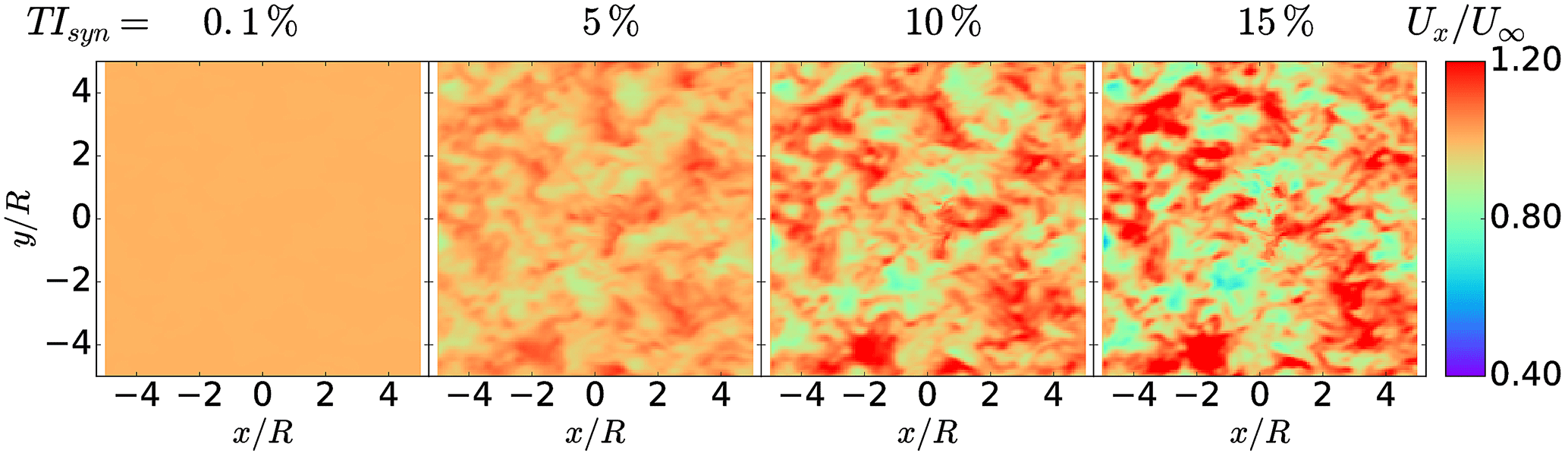
Figure 2 Midplane at $z/R=\mathrm{0}$ of the instantaneous normalized axial velocity component U_x∕U_∞ showing homogeneous isotropic turbulence for different turbulent intensities TI_syn in the numerical domain.

While the Glauert tip correction f_tip was originally intended (Glauert, 1935) to represent the otherwise absent tip vortices in the actuator disk model, it still proves advantageous for the ALM at lower resolutions as shown in Nathan (2018). Due to the relatively low resolution, the shed tip vortices from an ALM are much larger than the ones observed experimentally. Hence, the induction caused by the simulated vortices is weaker than in reality, and the Glauert tip correction permits us to compensate for it (Nathan et al., 2017).

Finally, in order to avoid spurious oscillations around the point of the inserted force, the punctual force is distributed using a kernel function $\mathcal{G}\cdot (\cdot )$. As done in previous works such as Troldborg (2009) or Olivares Espinosa (2017) this work adheres to a normal distribution with the distribution width ϵ=σΔx, with σ being the distribution width of the normal function and Δx the cell width.

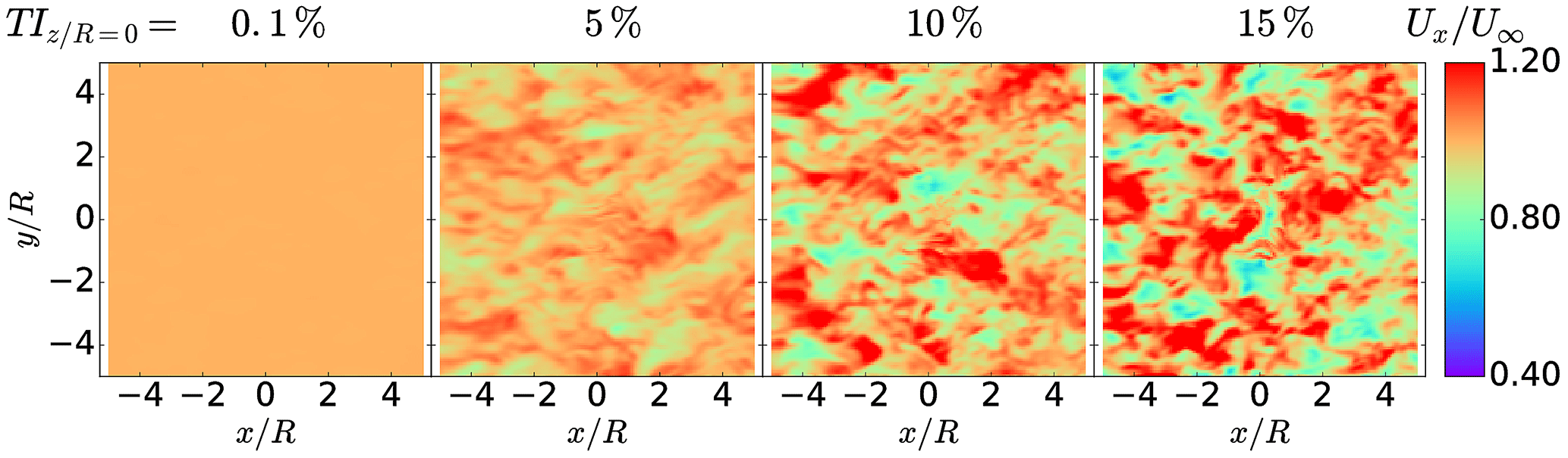
Figure 3 Horizontal plane of the instantaneous axial velocity component U_x in sheared flow for different longitudinal turbulence intensities TI${}_{z/R=\mathrm{0}}$ at hub position.

2.2 Turbulence inflow generation

2.2.1 Homogeneous isotropic turbulence

A synthetic velocity field representing homogeneous isotropic turbulence based on the von Kármán energy spectrum (Pope, 2000)

$$\begin{array}{}\text{(6)}& {\displaystyle }E\left(k\right)=\mathit{\alpha }{\mathit{ϵ}}^{\mathrm{2}/\mathrm{3}}{L}^{\mathrm{5}/\mathrm{3}}{\displaystyle \frac{L^{\mathrm{4}}{\mathit{\kappa }}^{\mathrm{4}}}{(\mathrm{1}+L^{\mathrm{2}}{\mathit{\kappa }}^{\mathrm{2}}{)}^{\mathrm{17}/\mathrm{6}}}}\end{array}$$

is obtained by using the algorithm proposed by Mann (1998). The technical details can be found in the article of Mann (1998) or more recently in Olivares Espinosa (2017). The main parameters for this approach are the integral length scale L and the coefficient αϵ^2∕3, which can be used as a scaling factor to obtain the desired amplitude of the turbulent structures. The range of wavenumber κ depends on the grid resolution and dimension extents. Hence, these parameters determine the ability of the numerical mesh to resolve a certain range of turbulent scales.

While several implementations of this method exist, e.g. Olivares Espinosa (2017) or Muller et al. (2014), the implementation of Gilling (2009) was chosen to synthesize the homogeneous isotropic turbulence (HIT) for several reasons. It is in public domain, it corrects for a divergence-free velocity field and allows us to impose HIT at the boundaries at relatively low computational cost.

In Fig. 2 the midplane of a generated turbulent field is shown for different turbulence intensities. The flow structures are identical apart from the different scaling of the velocity fluctuations. This results from using the same seed for the random number generator in the Mann algorithm and by scaling the obtained velocity field with αϵ^2∕3 to obtain the desired synthetic turbulence intensity TI_syn.

Contrary to Troldborg (2009) where the synthetic turbulence is imposed as a momentum source, in this work it is imposed as a boundary condition as done in Muller et al. (2014) and Olivares Espinosa (2017). The velocities are imposed by convecting the velocity field of the synthetic turbulence through the computational domain by the mean velocity U_∞ at each simulation time step. They are then projected by trilinear interpolation onto the computational points. In order to speed up the statistical convergence, the simulation is also initialized with the synthetic turbulence field.

2.2.2 Shear layer turbulence

Based on the Mann algorithm (Mann, 1998), Muller et al. (2014) developed a method to impose the synthetic turbulence on a sheared flow as boundary condition, including the evolution of the vortical structures. Apart from the turbulence intensity, no further turbulence characteristics were published by Schepers et al. (2012). Hence, a turbulence length scale of R∕4 was chosen. These scales were larger than the width of the coarsest cells in the numerical mesh in order to dampen the effect of numerical dissipation in axial direction. A typical flow field generated by this algorithm can be seen in Figs. 3 and 4.

Figure 4 Vertical plane of the instantaneous axial velocity component U_x in sheared flow for different longitudinal turbulence intensities TI${}_{z/R=\mathrm{0}}$ at hub position.

The mean velocity profile is obtained via the power law

$$\begin{array}{}\text{(7)}& {\displaystyle }{U}_x=U_{\mathrm{ref}}({\displaystyle \frac{z}{z_{\mathrm{ref}}}}{)}^{{\mathit{\alpha }}_p};\end{array}$$

hence, the velocity at the bottom of the domain has not necessarily got to be zero. Therefore, the computational mesh can be much smaller than in a wall-resolved flow, as its mesh has to include the ground and has to have a high refinement in this region. The reference height z_ref was set to hub height, and the reference velocity was set to U_ref=15 m s⁻¹. The parameter α_p can usually be deduced from experimental measurements if available. As they were not available for this experiment, standard conditions are assumed with ${\mathit{\alpha }}_p=\mathrm{1}/\mathrm{7}$ (Pope, 2000).

2.3 Numerical framework

This work is realized within the open-source framework OpenFOAM (version 2.2.2)¹ together with the SOWFA project,² which contains a similar implementation of the ALM as presented by Troldborg (2009). A more detailed explanation of the implementation can be found in Martínez-Tossas et al. (2016). OpenFOAM is a set of libraries and executables entirely written in C++. While the first released scientific article about the framework was by Weller et al. (1998), its inner workings are described in more detail by Jasak (1996).

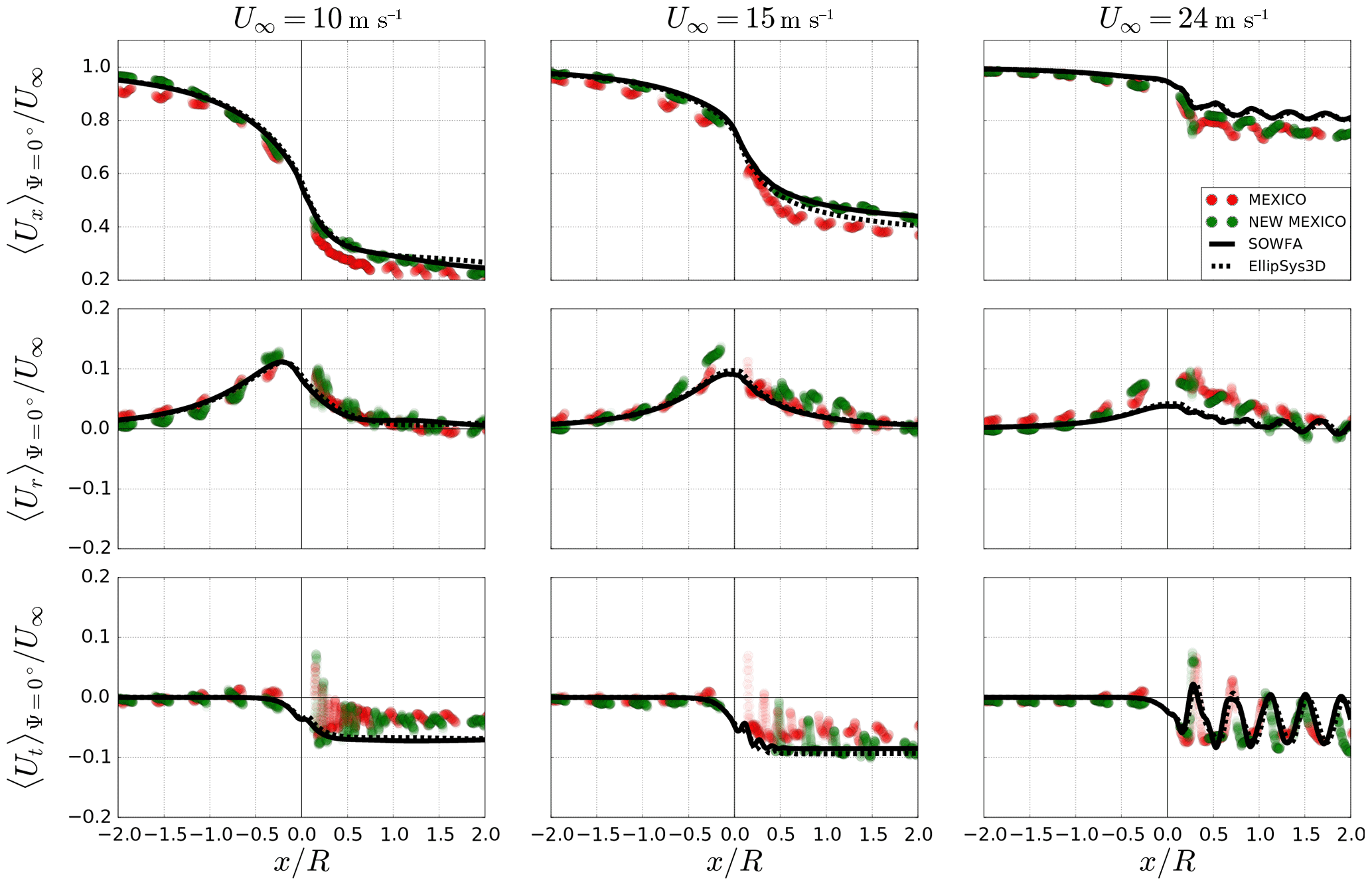
Figure 5 Axial profiles of phase-averaged (rotor position $\mathrm{\Psi }=\mathrm{0}{}^{\circ }$) velocity components normalized by the case-specific reference velocity U_∞. Three different flow cases for an outboard radial position are shown.

The computational domain is cubic with an edge length of $L_x=L_y=L_z=\mathrm{10}R$, with R being the rotor radius and the rotor positioned at the domain centre. The cells in the rotor vicinity are refined in the range of $-\mathrm{0.4}\le x/R\le \mathrm{0.4}$ with the size $\mathrm{\Delta }x=D/\mathrm{128}$. Within SOWFA, several refinement zones are applied, each time halving the cell edge length as also done in Vanella et al. (2008). The final mesh size consists of 1.9 × 10⁶ cells. The technique used in SOWFA proves highly advantageous in terms of computational cost. As the mesh dimensions at first sight seem relatively small compared to other work such as Troldborg (2009) or Martínez-Tossas et al. (2017), an extensive sensitivity study was conducted by varying domain extents in axial direction up- and downstream of the rotor as well as in the lateral direction for different grid refinements. The findings show that the dimensions used have a negligible impact as shown in Nathan (2018).

For the boundary conditions, the velocity is imposed as a uniform inflow velocity of $\mathbf{U}=(U_{\mathrm{\infty }},\mathrm{0},\mathrm{0})$ for the non-turbulent flow and in the turbulent cases as the synthetic velocity as explained in Sect. 2.2. The lateral boundaries are set as symmetric for the non-turbulent and homogeneous isotropic turbulence case. For the shear layer turbulence, the velocity is also imposed at the lateral boundaries.

The large eddy simulations use the dynamic Lagrangian sub-grid-scale model (Meneveau et al., 1996). For the discretization of the convective term, a linear combination of 75 % central differencing and 25 % second-order upwind scheme is applied as presented by Warming and Beam (1976). In OpenFOAM terminology, this scheme is called linear-upwind stabilized transport (LUST). The choice of the scheme is made as a trade-off between the accuracy of a linear discretization and the stability of an up-winding scheme. This scheme proved to preserve the turbulent structures well (Nathan, 2018). The remaining spatial terms are discretized by central differencing, and for the time discretization the Crank–Nicolson method is used.

The pressure is resolved using a geometric agglomerated algebraic multi-grid solver and the remaining variables are solved for with a bi-conjugate gradient method using a diagonally based incomplete LU preconditioner. The total simulation run-time comprises 60 rotor revolutions (≈8.5 s), and the time step has to be small enough to avoid the actuator point representing the blade tip skipping a computational cell during rotation. It is set to $\mathrm{0.327}\times {\mathrm{10}}^{-\mathrm{3}}$ s. The total run-time is chosen as first- and second-order statistics are deemed to be converged.

For the parameterization of the ALM, different distribution widths are chosen in order to obtain the optimum for the examined case and 40 actuator points are used to represent one blade in accordance with what was found in Nathan (2018).

3 Results

3.1 Validation and verification

The implementation was validated against EllipSys3D and verified against the Model Experiment in Controlled Conditions (MEXICO) and New Model Experiment in Controlled Conditions (NEW MEXICO) experiment in Nathan et al. (2017). The MEXICO rotor is a three-bladed rotor with a radius R=2.25 m. It rotates at a constant rpm of 424.5 min⁻¹ for the three different flow cases with $U_{\mathrm{\infty }}=\mathit{\{}\mathrm{10},\mathrm{15},\mathrm{24}\mathit{\}}$ m s⁻¹; hence, their respective tip speed ratios are 10.0, 6.7 and 4.2. As shown in Nathan (2018), the chord-based Reynolds number $Re=U_{\mathrm{\infty }}c/\mathit{\nu }$ varies from 0.4×10⁶ for the low-velocity case towards the hub up to 0.6×10⁶ for the high-velocity case in the tip region. The power coefficients for the observed cases are $C_{\mathrm{P}}=\mathit{\{}\mathrm{0.28},\mathrm{0.36},\mathrm{0.19}\mathit{\}}$. A comparison of the axial profiles of the velocity components can be seen (Fig. 5) showing that both codes reproduce very similar results in the near wake further away from the rotor. Apart for the high-velocity case where 3-D effects become important, an excellent agreement can be observed for the other two cases.

For the high-velocity case (U_∞=24 m s⁻¹), the vortex sheets shed from the blades become visible by the oscillations in the axial velocity component U_x.

3.2 Non-turbulent flow

When refining the grid using the actuator line method, the distribution parameter ϵ has to be adjusted to obtain a global torque 〈T〉 close to the reference value T_ref. In the following, only the case for U_∞=15 m s⁻¹ will be examined as the other cases in Nathan et al. (2017) served as extreme cases for determining how the model behaves at its limits.

Instead of relying on a constant ϵ∕Δx for different grid resolutions, this work adapts ϵ∕Δx depending on the grid resolution or number of cells across the rotor diameter $N=\mathrm{2}R/\mathrm{\Delta }x$. The results are shown in Eq. (6). A confidence interval of ±1 % was established around the reference torque value T_ref. Through iterations, an optimal distribution parameter is found to fall in this range.

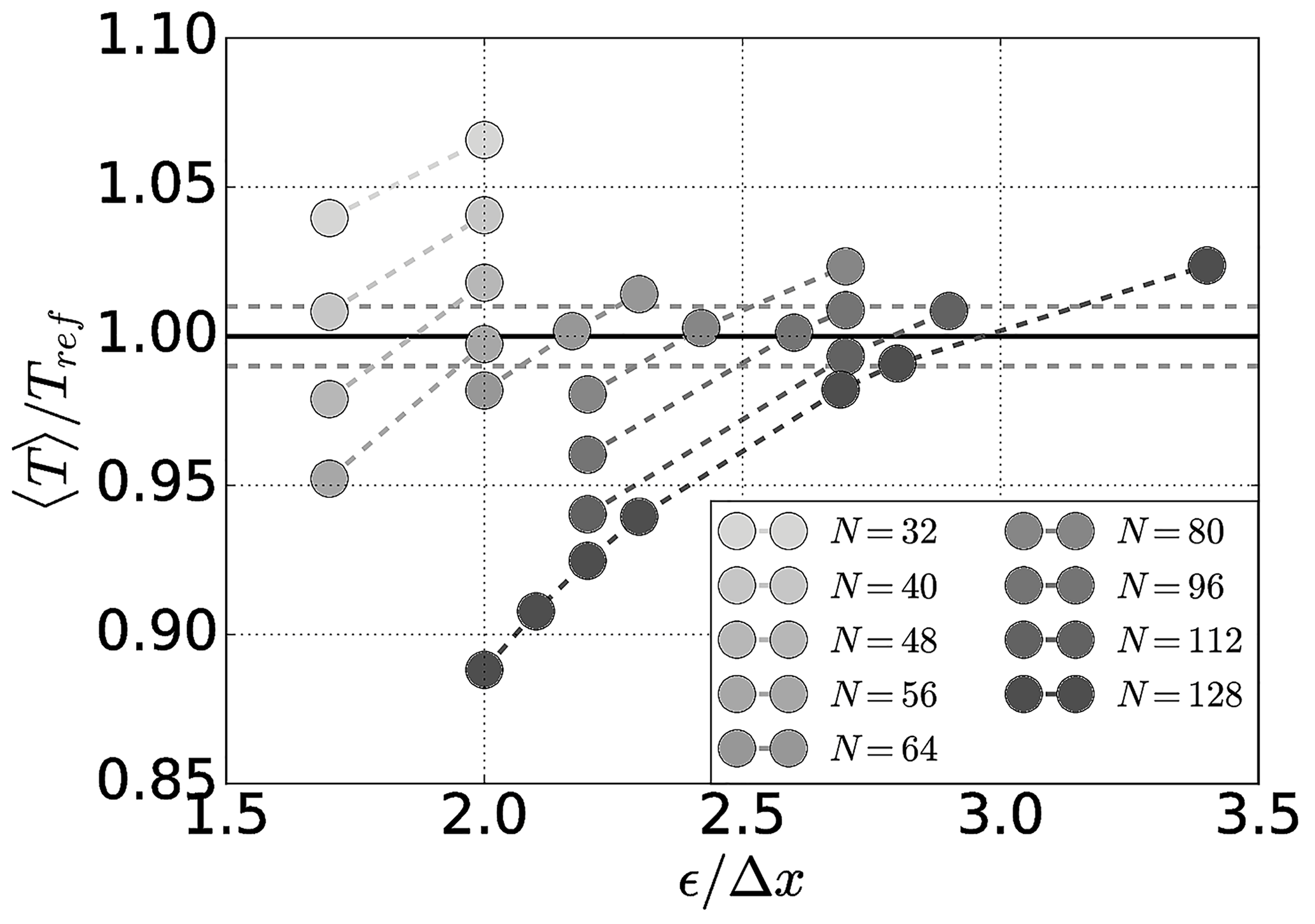
Figure 6 Relation between ϵ∕Δx and the resulting global torque normalized by the reference torque for U_∞=15 m s⁻¹.

The lower bound for the distribution parameter here is ϵ=1.7Δx for the sake of the numerical stability of the applied method. Other frameworks applying a different numerical discretization can go even lower, e.g. in Ivanell et al. (2010). By doing so, it can be seen that the best solution in terms of global torque for a resolution of $N=D/\mathrm{\Delta }x=\mathrm{32}$ is off by around 4 % in Fig. 6.

As a general trend, it can be seen that ϵ∕Δx has to be increased with increasing resolution. This stems from the fact that by refining the mesh with a constant ϵ∕Δx, the punctual induction caused by the blade would be too high and eventually the torque would be below the reference value, e.g. for ϵ=2Δx for N≥64. By contrast, when having a very low resolution, a constant ϵ distributes the force too widely, causing a lower induction around the rotor resulting in an overestimation of the torque, e.g. for ϵ=2Δx for N≤48.

The optimal distribution parameter ϵ∕Δx found in Fig. 6 is now shown in dependence on the grid resolution $N=D/\mathrm{\Delta }x$ in Fig. 7. It seems as if this value would eventually reach an asymptotic limit for higher resolutions. Looking at a more theoretical approach in Martínez-Tossas et al. (2017) suggests that the optimal distribution width ϵ lies between 0.14 and 0.25 of the chord c whereas in this case for $D/\mathrm{\Delta }x=\mathrm{128}$ the ϵ∕c lies between 0.5–8.9 depending on the span-wise location. The observation made by Martínez-Tossas et al. (2017) is backed by Shives and Crawford (2013), where ϵ∕c falls in the same range. But it should be kept in mind that Shives and Crawford (2013) use a much higher grid resolution, allowing $\mathit{ϵ}/\mathrm{\Delta }x\ge \mathrm{4}$ and in the case of Martínez-Tossas et al. (2017) even $\mathit{ϵ}/\mathrm{\Delta }x\ge \mathrm{5}$.

Figure 7 Optimal ϵ∕Δx over number of cells for resolving one rotor diameter D∕Δx.

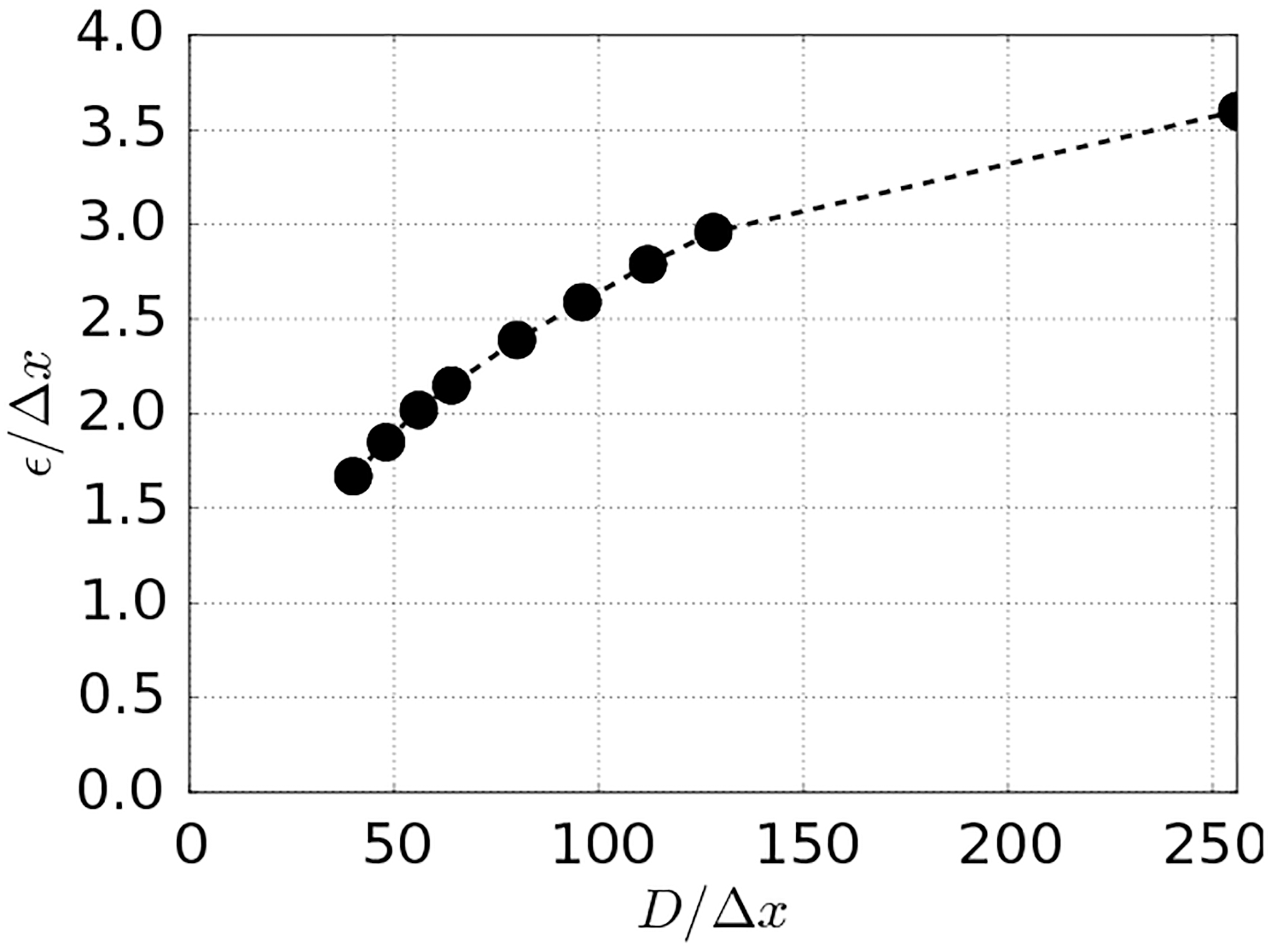
The curvature in Fig. 7 also confirms the findings of Jha et al. (2013) that keeping the relation $\mathit{ϵ}/\mathrm{\Delta }x=\mathrm{const}$ while increasing the resolution is not a very good solution. While Ivanell et al. (2010) suggests choosing the smallest possible distribution width ϵ in order to minimize interactions with the vortical structures ($\mathit{ϵ}/\mathrm{\Delta }x=\mathrm{1}$), the observations made here fall more in line with work such as Shives and Crawford (2013), suggesting ϵ∕Δx to be adapted to the physical model in order to distribute the force over a meaningful length scale.

For an excerpt of the resolutions presented in Fig. 6, the radial profiles of the velocity components can be found in Fig. 8. It can be seen that the method seems to converge towards a solution when refining the mesh. As shown in Fig. 6 the lowest resolution at N=32 over-predicts the torque by distributing the force to widely, which is also reflected in the low axial induction downstream at $x/R=\mathrm{0.13}$. Despite following the trend of the experimental values well, the method seems to converge towards radial profiles which are especially off in the tip and hub region where the strongest vortices are shed. These are limitations intrinsic to the ALM, which is less apparent when using high-fidelity approaches such as full rotor simulations (Carrión et al., 2015). In order to ameliorate the results at the tip, a non-isotropic kernel could be investigated (Rullaud et al., 2018).

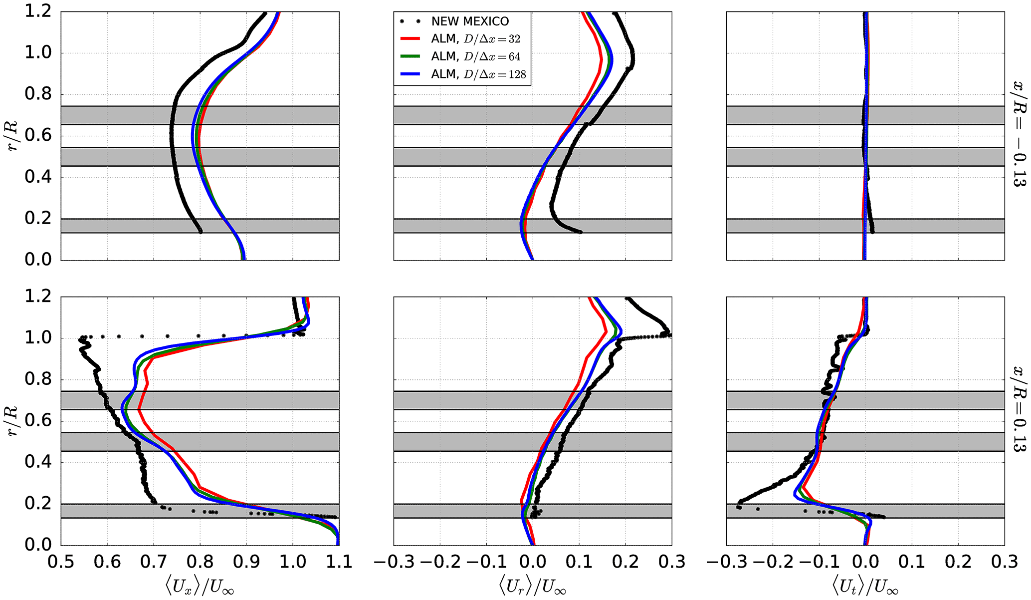
Figure 8 Radial profiles of time-averaged velocity components 〈U_x〉 (axial), 〈U_r〉 (radial) and 〈U_t〉 (tangential) for ALM in different grid resolutions at $x/R=\mathrm{0.13}$.

In Fig. 9 the shed vortical structures can be seen in dependence on the grid resolution. While the root vortex is rather diffuse, a clear tip vortex can be noticed. It is interesting to note the vortices shed around mid-span due to the suboptimal choice of the airfoils of the blade causing a sudden change in circulation.

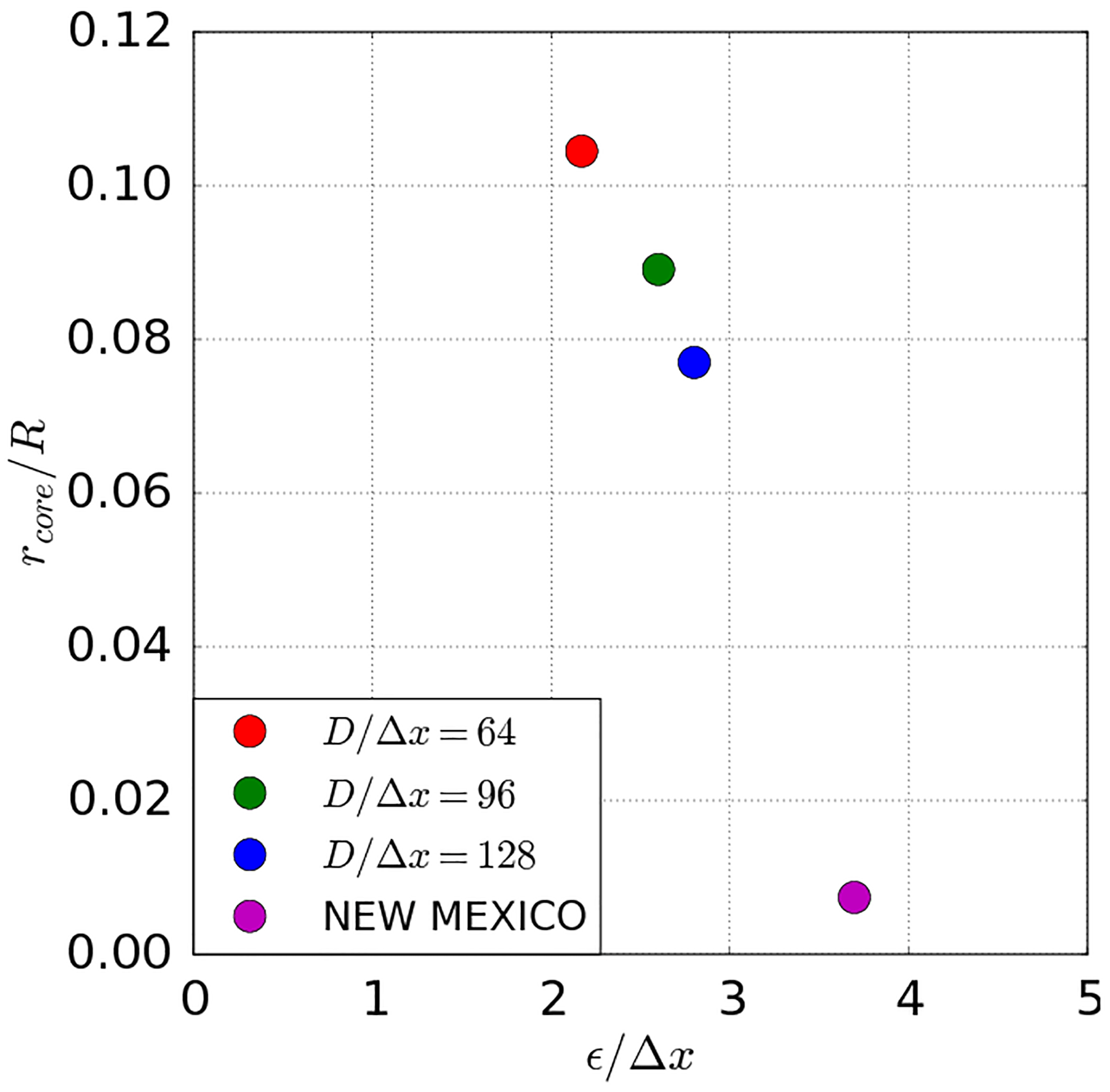
In order to estimate the resolution necessary to obtain tip vortex radii as seen in the MEXICO experiment, the vortex radii are shown in Fig. 10. The vortex radius r_core is defined as the limit containing 99 % of the circulation. The Gaussian distribution is used as an approximation for the vorticity distribution within the vortex. This assumption is normally applied for low Reynolds number flows, while this case exhibits a Reynolds number of $R{e}_{\mathrm{\Gamma }}=\mathrm{\Gamma }/\mathit{\nu }=\mathrm{220}\times {\mathrm{10}}^{\mathrm{3}}$. As these findings are related to the vortex dynamics of the flow Re_Γ is used instead of Re defined earlier. Nevertheless, this approximation is used in order to be able to draw an analogy between the experimental and the numerical results. It holds fairly well when comparing the Gaussian distribution and the vorticity for N=128 as shown in Nathan (2018). Hence, by assuming a Gaussian distribution for the vortices in the MEXICO experiment, a corresponding distribution parameter ϵ can be deduced as shown in Fig. 10.

This would necessitate a resolution of N≥4096 for the presented case, which would result in a computational grid beyond any justifiable computational scope. Full rotor calculations as conducted by Carrión et al. (2015) allowed us to obtain tip vortices of $r_{\mathrm{core}}/R\approx \mathrm{0.012}$ for N≈900 in the tip region, which corresponds very well to results in Fig. 10. Another result for the vortex radius can be found in Nilsson et al. (2015), where for $\mathit{ϵ}/\mathrm{\Delta }x=\mathrm{1}$ and N≈244 in the tip region a vortex core radius of $r_{\mathrm{core}}/R\approx \mathrm{0.055}$ was found. Despite the radii in this work and the references being calculated based on three different methods, the results fall within the same range.

Figure 9 Normalized vorticity $\langle \mathit{\omega }{\rangle }_{\mathrm{\Psi }=\mathrm{0}{}^{\circ }}/\langle \mathit{\omega }{\rangle }_{\mathrm{\Psi }=\mathrm{0}{}^{\circ },max}$ in the near wake for different grid resolutions.

Figure 10 Normalized vortex radius r_core∕R over normalized distribution parameter ϵ∕Δx.

3.3 Homogeneous isotropic turbulence

In Fig. 11 the longitudinal evolution of the turbulence intensities can be seen. There is a stronger decay for higher turbulence intensities, which was also found in Olivares Espinosa (2017). In that work EllipSys3D was compared to a solution based on OpenFOAM, and it was found that over the same longitudinal distance of 10R an absolute difference in the turbulence intensity of 48 % and 44 % occurred for each framework respectively. This stands in a stark contrast to the 4 % in this case for the high turbulence-intensity case. This huge decay, which is even more significant for EllipSys3D, necessitates approaching the introduction of the turbulence close to the turbine for high turbulence-intensity cases (Olivares Espinosa, 2017).

An important aspect when imposing a synthetic turbulence as boundary conditions of a Computational Fluid Dynamics (CFD) simulation is respecting the Nyquist–Shannon sampling theorem (Shannon, 1949) as also mentioned by Muller et al. (2014). Hence, a study considering different ratios between the grid resolution of the synthetic turbulence and the simulation was undertaken. It is found that the higher the computational resolution is compared to the one of the synthetic turbulence, the less the turbulence intensity decays in longitudinal direction. While the criterion of Nyquist–Shannon states that the resolution of the computational domain should be d$x/\mathrm{\Delta }x>\mathrm{2}$, this work uses the ratio of d$x/\mathrm{\Delta }x=\mathrm{2.5}$, with dx being the cell width of the synthetic field and Δx the cell width of the computational mesh.

When taking the case for TI_syn=5 %, it is interesting to note that while the resolved TI (green dashed line) is around 4.2 % at the rotor position $x/R=\mathrm{0}$, a huge part of the difference in relation to the imposed turbulence falls in the SGS model with $\langle {\mathrm{TI}}_{\mathrm{res}}\rangle +\langle {\mathrm{TI}}_{\mathrm{sgs}}\rangle =\mathrm{4.8}$ % and finally just a relatively small amount of the turbulent intensity or turbulent kinetic energy is “lost” by numerical dissipation.

Despite the fact that the computational grid respects the Nyquist–Shannon criterion for signal sampling in respect to the synthetic grid, immediately at the inlet a part of the turbulence falls in the sub-grid range. Due to the numerical dissipation caused by the differencing schemes and turbulence modelling, the energy cascade hands down its energy to lesser scales than the resolved ones.

It should be kept in mind, that the turbulence intensity the rotor model is experiencing through velocity sampling is the resolved turbulence intensity TI_res, and the sub-grid turbulence intensity TI_sgs is therefore only felt indirectly, by an augmentation of the effective viscosity. When looking at the fraction of the resolved turbulent kinetic energy over the total turbulent kinetic energy, it can be seen that the resolved scales exceed 96 %, which lies well above the criterion of 80 % proposed by Pope (2004). For the flow case with U_∞=15 m s⁻¹, the total simulation run-time t_tot results in roughly $t_{\mathrm{tot}}\cdot U_{\mathrm{\infty }}/\left(\mathrm{10}R\right)\approx \mathrm{5.5}$ flow through times. The synthetic turbulence field is large enough that it does not need to be recycled during one simulation.

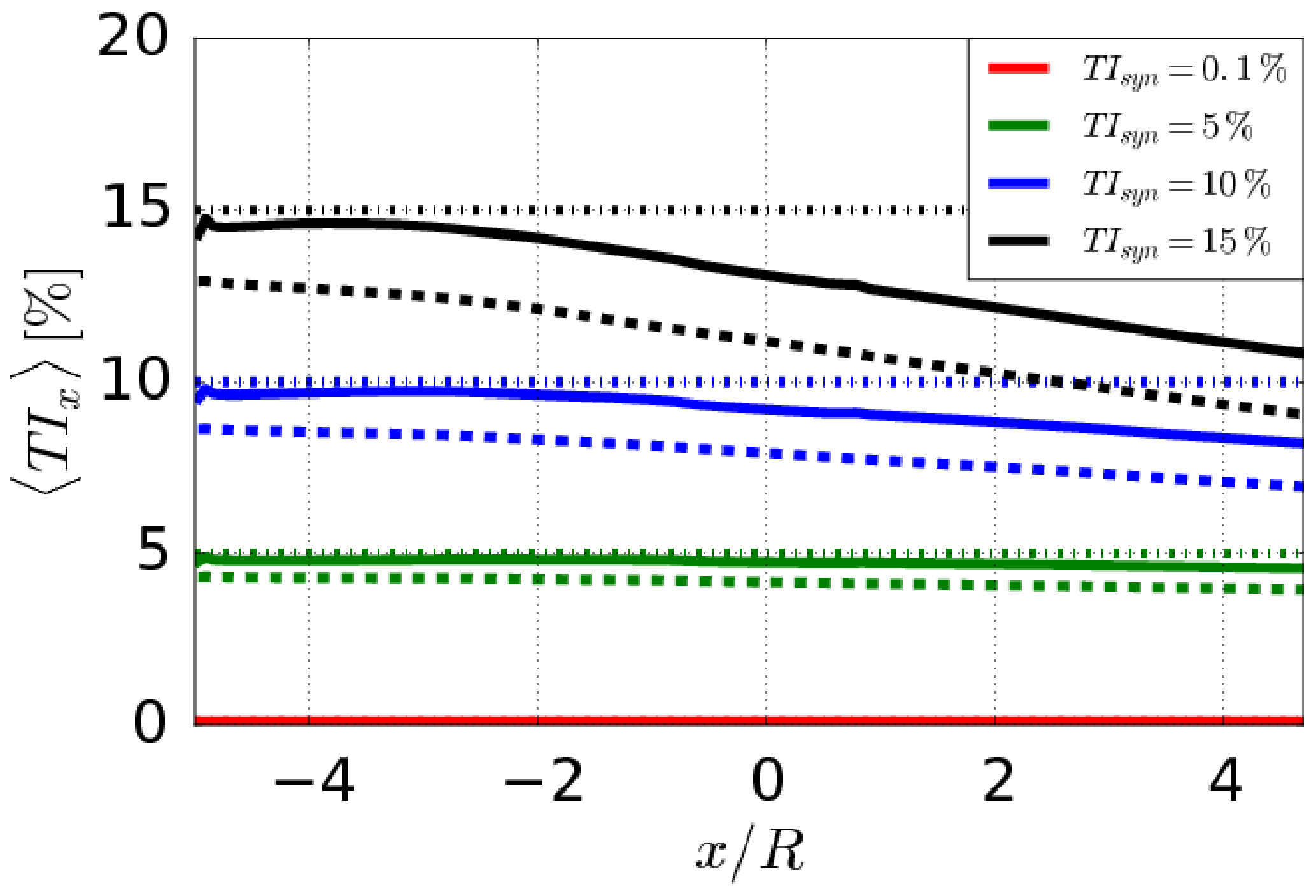
Figure 11 Longitudinal evolution of turbulence intensities for different turbulent intensities at the inlet in HIT without rotor effects. For each case the mean value 〈TI〉 is shown with the resolved TI 〈TI_res〉 (dashed line), resolved and subgrid scale TI 〈TI_res〉+〈TI_sgs〉 (solid line), and the inlet TI TI_syn (dotted line) as reference. The sudden spike at the end of the domain is caused by the outlet condition, and its influence is restricted to the last computational cell before the outlet.

In Fig. 12 the effects of the ambient turbulence on the turbine wake are shown. While there are no noticeable impacts for the low-turbulence case with TI_syn=0.1 %, the beginning of strong non-linear interactions can be observed for TI_syn>0.1 %. For TI_syn=15 % the inflow turbulent structures seem to outgrow the structures created by the wind turbine.

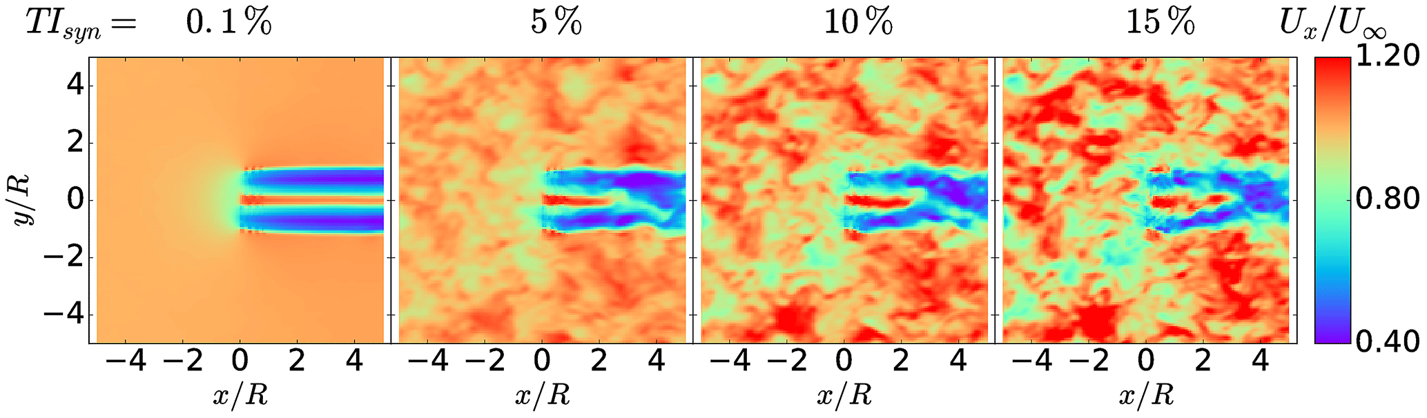
Figure 12 Normalized instantaneous axial velocity component U_x∕U_∞ of wind turbine wake immersed in HIT for different turbulence intensities.

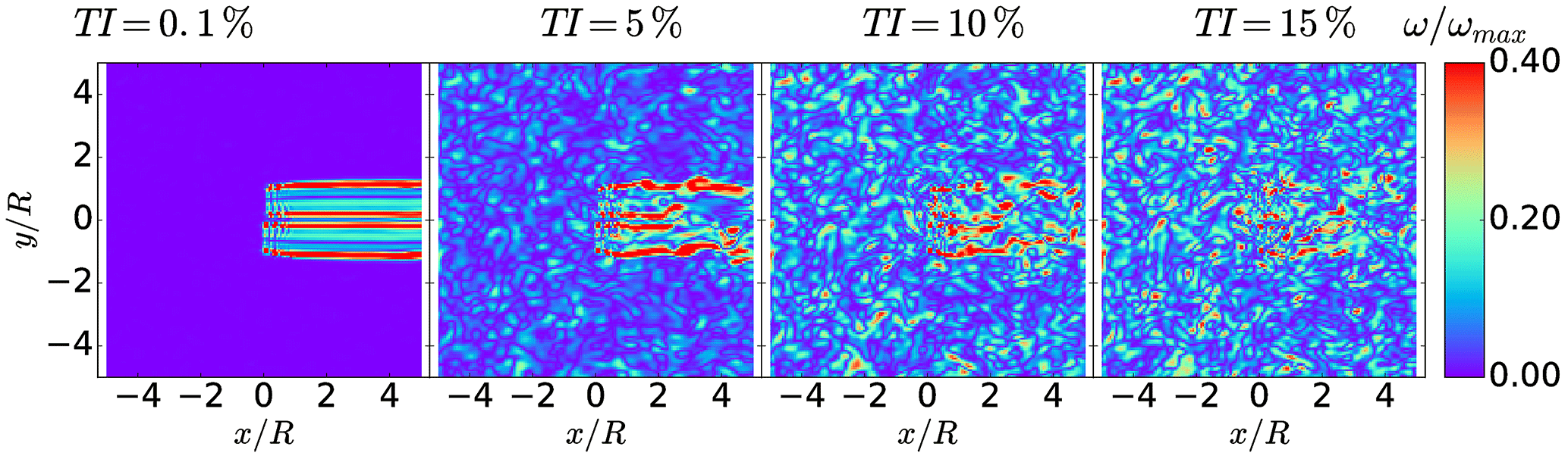
Figure 13 Normalized instantaneous vorticity ${\mathit{\omega }}_x/{\mathit{\omega }}_{max}$ of wind turbine wake immersed in HIT for different turbulence intensities.

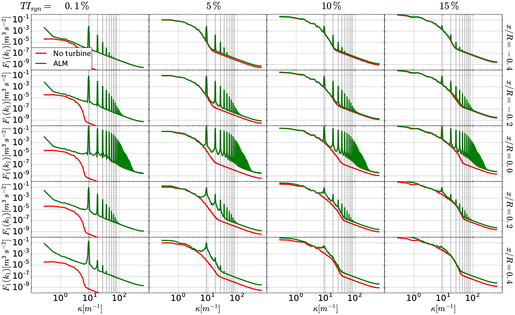
Figure 14 The energy spectra for the HIT based on the time series of the axial velocity component at different points in the near wake ($x/R=\mathit{\{}-\mathrm{0.4},-\mathrm{0.2},\mathrm{0},\mathrm{0.2},\mathrm{0.4}\mathit{\}}$) for different inlet turbulent intensities $T_{\mathrm{syn}}=\mathit{\{}\mathrm{0.1},\mathrm{5},\mathrm{10},\mathrm{15}\mathit{\}}$ % are shown. The impact of the rotor presence can be seen by the spikes at the wavenumber 3 times the rotor frequency and its higher harmonics (dotted black lines).

In Fig. 13 it can be seen how the strength of the vortical structures of the ambient fluid increases with higher turbulence intensity up to the point for T_syn=15 % where its amplitude almost equals the one emitted by the rotor model. In Fig. 14 the impact of the rotor presence on the energy spectrum can be seen. The wavenumber κ_p relating to the frequency of a blade passage (3 times rotor frequency) obtained by ${\mathit{\kappa }}_{\mathrm{p}}=\mathrm{2}\mathit{\pi }\mathrm{3}f/U_{\mathrm{\infty }}$ shows a very distinct peak and its higher harmonics at the multiples of κ_p.

As the velocity time series obtained from the simulations do not exhibit periodicity, the Welch method (Welch, 1967) is used to generate the energy spectra.

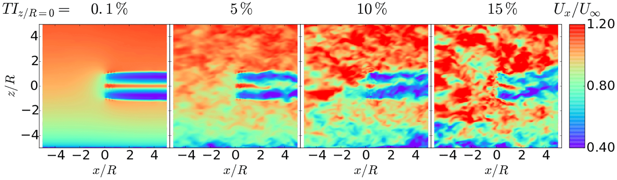
Figure 15 Vertical plane of the instantaneous axial velocity component U_x of wind turbine wake immersed in shear turbulent flow.

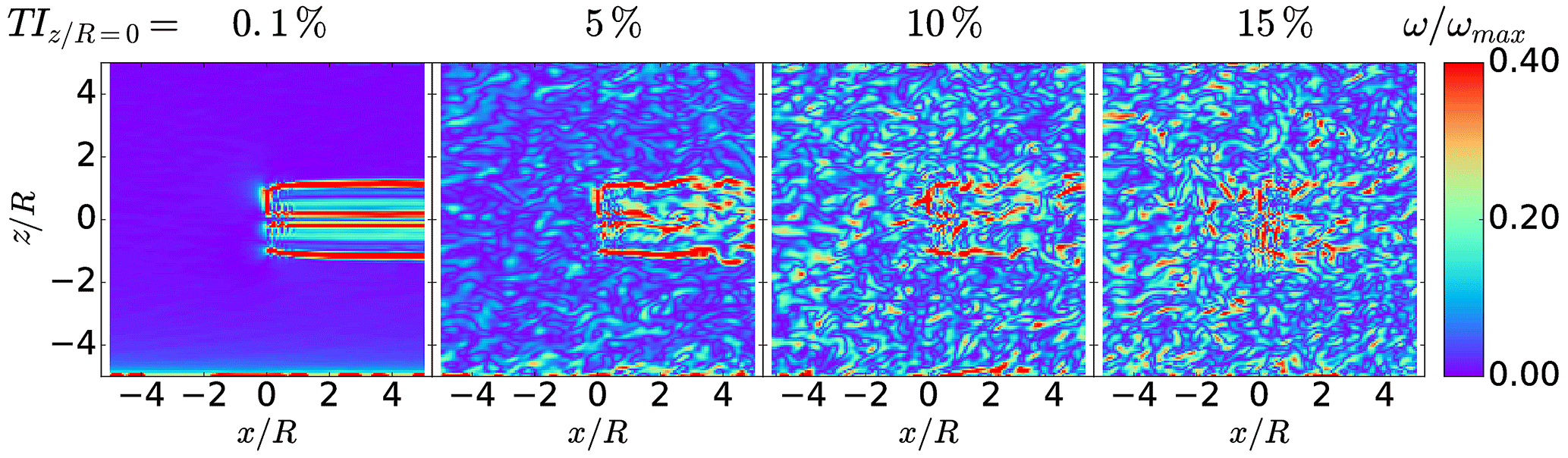
Figure 16 Instantaneous normalized vorticity $\mathit{\omega }/{\mathit{\omega }}_{max}$ in sheared flow for different longitudinal turbulence intensities TI_x at hub position. Vertical plane at $y/R=\mathrm{0}$.

It is interesting to note that the distinct peaks in the spectra occur at the wavenumber relating to the frequency of the blade passage and its harmonics. The harmonics are caused by the strong excitement of the fluid by the blade passage and its interaction with the non-linear term in the NS equations. As the blade forces and hence the strength of the tip vortices are very comparable, the peaks are very similar among the different cases for $-\mathrm{0.4}\le x/R\le \mathrm{0.2}$. The higher the turbulent kinetic energy content stemming from the ambient flow, the faster the peaks are dampened and blend into the ambient flow. For example there is almost no discernible effect by the blade at $x/R=\mathrm{0.4}$ for TI_syn=15 % while for TI_syn=0.1 % the velocity oscillations are still very noticeable. Although it is of lesser amplitude, the upstream region is also under the influence of the distinct blades to a certain extent.

3.4 Shear layer turbulence

When looking at the vertical planes in Fig. 15, the influence of the sheared flow can be seen by a higher velocity deficit in the wake on the lower half of the rotor. In the vertical plane in Fig. 16, it can be seen that there is an increase in the vorticity magnitude towards the ground. While the increase appears to be rather subtle, it is shown in Nathan (2018) that the TI increases significantly towards the ground as expected in a shear layer flow. Looking at the energy spectra in Fig. 17 reveals a similar picture as shown above for the case of homogeneous isotropic turbulence. As the blade forces and hence the strength of the tip vortices are very comparable, the peaks are very similar among the different cases for $-\mathrm{0.4}\le x/R\le \mathrm{0.2}$. Due to the dissipation caused by the ambient turbulence, these peaks dampen at a different pace as seen at $x/R=\mathrm{0.4}$.

While before and at the rotor position for $-\mathrm{0.4}\le x/R\le \mathrm{0}$ the peaks remain very distinct, vortical structures by the ambient fluid and emitted by the blade cause the injected peaks to dampen and distribute energy to adjacent wavenumbers as seen clearly for $x/R\ge \mathrm{0.2}$. Depending on the level of the ambient turbulence the peak gets attenuated up to a point where it almost completely blends in with ambient turbulence as seen for TI${}_{x,z/R=\mathrm{0}}=\mathrm{15}$ % at $x/R=\mathrm{0.4}$. This relates to the observation made earlier that ambient structures are almost as important as the structures emitted by the blade.

This means that in the near wake in a turbulent flow with an ambient turbulence intensity of TI${}_{x,z/R=\mathrm{0}}\ge \mathrm{10}$ %, the velocity fluctuations at $x/R=\mathrm{0.4}$ already seem to have only a weak relation to the injected turbulence by the rotor but a much stronger one to the ambient turbulence. This means that for this kind of flow, an actuator disk method would probably also be sufficient when looking at the flow characteristics beyond $x/R=\mathrm{0.4}$.

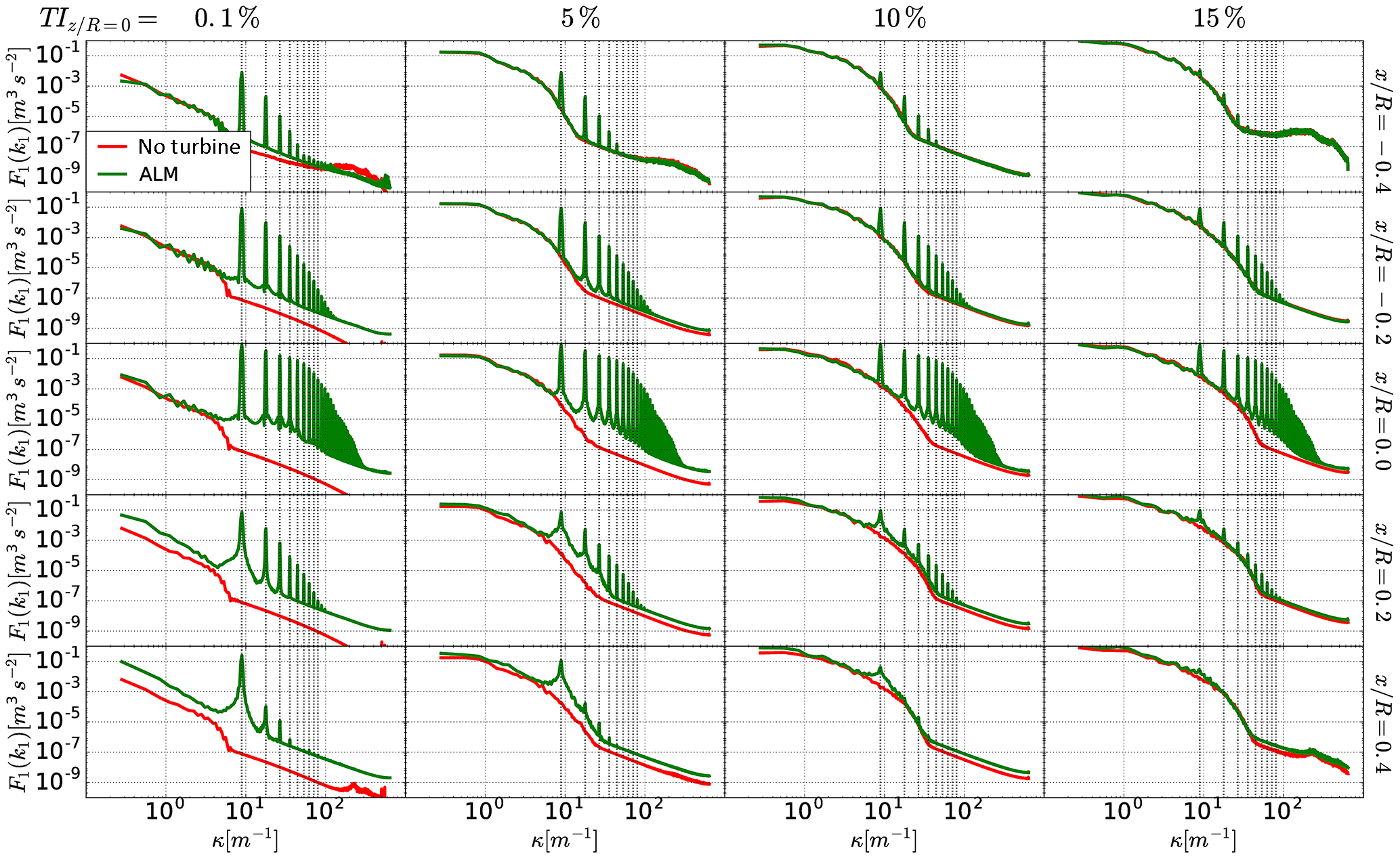
Figure 17 The energy spectra for the shear layer flow based on the time series of the axial velocity component at different points in the near wake ($x/R=\mathit{\{}-\mathrm{0.4},-\mathrm{0.2},\mathrm{0},\mathrm{0.2},\mathrm{0.4}\mathit{\}}$) for different inlet turbulent intensities $T_{\mathrm{syn}}=\mathit{\{}\mathrm{0.1},\mathrm{5},\mathrm{10},\mathrm{15}\mathit{\}}$ % at hub height $z/R=\mathrm{0.0}$ are shown. The impact of the rotor presence can be seen by the spikes at the wavenumber 3 times the rotor frequency and its higher harmonics (dotted black lines).

4 Conclusions

By using a validated actuator line implementation (Nathan et al., 2017), it was shown that the distribution width ϵ∕Δx has a non-linear dependence on the grid resolution and probably converges towards values suggested in Martínez-Tossas et al. (2016). The rotor torque is used as a global indicator for determining the distribution width, but the rotor thrust followed the same trend. Hence, it is interesting to see that while the rotor induction is predicted well, the velocity deficit agrees well only for $x/R>\mathrm{5}$ but not in the ultimate rotor vicinity.

It is also shown that with increasing grid resolution the spatial profiles seem to converge. This would be one aspect of a grid-independent solution, but it is still very far away from resolving the shed tip vortices correctly. Although it seems to converge towards a value of $\mathit{ϵ}/\mathrm{\Delta }x\approx \mathrm{4}-\mathrm{5}$ for which the dimensions of the experimental vortices would be attained, this causes excessive computational costs due to the large mesh.

When looking at the turbulent inflow, a synthetic turbulence generated by the Mann algorithm (Mann, 1998), it was shown that the decay of the turbulence intensity in longitudinal direction is much less pronounced than in previous work. As shown for the axial decay of the turbulence intensity, a significant part of the difference between the resolved turbulence intensity and the imposed one from the synthetic field resides within the sub-grid scales. Hence, there is very little loss due to numerical dissipation, which is also reflected in the energy spectra, which are the better the higher the turbulent content is.

As expected the wake does recover at a faster pace for a higher turbulence intensity. It is very interesting to note that the turbulent structures of the ambient flow eventually catch up with the amplitude of the structures emitted by the rotor. This is already noticeable in the instantaneous velocity fields but becomes even clearer when evaluating the spectra. When considering the velocity fluctuations in the downstream flow caused by the blade passages for determining the near wake, it can be observed that in this case for TI_syn≥10 %, the near wake already ends at $x/R=\mathrm{0.4}$. This is particularly interesting as a turbulence intensity of 15 % at hub height is still considered to be low turbulence intensity according to ISO 61400 (2015), and many real sites exhibit even higher turbulence intensities. Hence, for some cases, the limit of the near wake would be $x/R=\mathrm{0.4}$ and even lower.