the Creative Commons Attribution 4.0 License.
the Creative Commons Attribution 4.0 License.
 | 03 Apr 2019
Multipoint high-fidelity CFD-based aerodynamic shape optimization of a 10 MW wind turbine
Frederik Zahle
Niels N. Sørensen
Joaquim R. R. A. Martins
The wind energy industry relies heavily on computational fluid dynamics (CFD) to analyze new turbine designs. To utilize CFD earlier in the design process, where lower-fidelity methods such as blade element momentum (BEM) are more common, requires the development of new tools. Tools that utilize numerical optimization are particularly valuable because they reduce the reliance on design by trial and error. We present the first comprehensive 3-D CFD adjoint-based shape optimization of a modern 10 MW offshore wind turbine. The optimization problem is aligned with a case study from International Energy Agency (IEA) Wind Task 37, making it possible to compare our findings with the BEM results from this case study and therefore allowing us to determine the value of design optimization based on high-fidelity models. The comparison shows that the overall design trends suggested by the two models do agree, and that it is particularly valuable to consult the high-fidelity model in areas such as root and tip where BEM is inaccurate. In addition, we compare two different CFD solvers to quantify the effect of modeling compressibility and to estimate the accuracy of the chosen grid resolution and order of convergence of the solver. Meshes up to 14×106 cells are used in the optimization whereby flow details are resolved. The present work shows that it is now possible to successfully optimize modern wind turbines aerodynamically under normal operating conditions using Reynolds-averaged Navier–Stokes (RANS) models. The key benefit of a 3-D RANS approach is that it is possible to optimize the blade planform and cross-sectional shape simultaneously, thus tailoring the shape to the actual 3-D flow over the rotor. This work does not address evaluation of extreme loads used for structural sizing, where BEM-based methods have proven very accurate, and therefore will likely remain the method of choice.
- Article
(9009 KB) - Full-text XML
- BibTeX
- EndNote


Wind turbine rotor optimization aims to maximize wind energy extraction and has been an important area of research for decades. A common metric is to minimize the levelized cost of energy (LCoE) (Ning et al., 2014), which can be decreased by lowering installation costs and operating expenses or by increasing the annual energy production (AEP). Simply upscaling the turbine leads to an increase in swept area, which in turn extracts more energy. However, a naive upscaling does not capture the complexity of the problem (Ashuri, 2012).
A major drawback of naive upscaling is that mass increases with the cube of the rotor radius. The industry avoids the prohibitive mass increase by improving the blade design, which has resulted in blades that are more slender for a given power rating, where the increase in loads (and therefore mass) can be kept low. This further results in blades with increased capacity factors.
Traditionally, the blade design optimization process has been sequential, where the optimization of airfoils and planform are performed in two distinct steps. In the present work, we optimize the airfoils and the planform concurrently using 3-D computational fluid dynamics (CFD). This concurrent design optimization process is vital for the industry because, as previously shown, concurrent design processes result in a larger gain compared to sequential counterparts (Barrett and Ning, 2018), which is the main principle in multidisciplinary design optimization (MDO) (Martins and Lambe, 2013).
The use of 3-D CFD is particularly valuable near the turbine blade root and tip, since the blade element momentum (BEM) method uses empirical models to capture 3-D effects for these regions. The increase in fidelity also allows us to explore out-of-plane features such as blade pre-bend and winglets, which is outside the scope of traditional BEM approaches.
Industry still relies heavily on BEM, given that the 3-D CFD shape design of rotors poses several challenges. One of these challenges is modeling all the load cases that drive the design during an optimization. Much work has been done in steady-state computations with steady uniform inflow, but to truly generate realistic loads, one should transition to turbulent inflow and accurately resolve the time domain. This poses an immense challenge in terms of memory and computation time and is an active area of research.
In this paper, we present results from a high-fidelity aerodynamic shape optimization of a 10 MW offshore wind turbine rotor. By “high-fidelity”, we mean a detailed modeling of the rotor in 3-D and the use of Reynolds-averaged Navier–Stokes (RANS) equations to model the aerodynamics throughout the optimization. The optimization is based on the case study from the International Energy Agency (IEA) Wind Task 371, which allows for a comparison with the low-fidelity BEM results from this case study. Low-fidelity tools offer a fast and reliable modeling approach. However, BEM does not capture the physics as completely as high-fidelity CFD-based tools that solve the RANS equations. In the present work, we aim to quantify the pros and cons of each approach.
Ideally, one would include all the relevant disciplines in such an optimization. This has been addressed in previous work using BEM-based aeroelastic tools combined with various cross-sectional analytical or finite-element-based structural tools.
Zahle et al. (2016) showed that simultaneous design of the aerodynamic shape and structural layout of a blade leads to passive load alleviation. This was achieved through bend–twist coupling, which increased the AEP without increasing loads and blade mass. The LCoE has been minimized by other researchers while taking aerodynamics, structures, and controls into account, thereby truly treating it as an MDO problem both for 5 MW turbines (Ashuri et al., 2014) and for 20 MW turbines (Ashuri et al., 2016). While we could tackle high-fidelity aerostructural optimization using tools that have already been demonstrated in aircraft wing design (Kenway and Martins, 2014; Brooks et al., 2018; Kenway et al., 2014), we focus solely on aerodynamic shape optimization in the present work.
We start the remainder of this paper with a literature review on wind turbine optimization. We then explain the methodology (Sect. 3), followed by a comparison between the compressible flow solver and an incompressible flow solver (Sect. 4). The design optimization problem is presented in Sect. 5, followed by the optimization results in Sect. 6. We end with our conclusions in Sect. 7.
This literature review on wind turbine optimization is divided into three overall approaches: those that use low-fidelity and multi-fidelity models (Sect. 2.1), approaches that use CFD models without adjoint sensitivities (Sect. 2.2), and approaches that use CFD models with adjoint solvers (Sect. 2.3).
2.1 Low-fidelity and multi-fidelity shape optimization
CFD-based aerodynamic shape optimization is still rarely used in wind energy research, but both the aerospace and the automotive communities have been using it increasingly often (Chen et al., 2016; He et al., 2018). However, when it comes to low-fidelity shape optimization, the wind energy community has a large body of work.
BEM codes have been used extensively throughout the wind energy community for aerodynamic optimization. These codes are easy to implement and incur low computational cost. Robustness has been an issue in BEM codes, as they do not always converge (Maniaci, 2011). Robustness is critical, especially when the analysis is part of an optimization cycle. A lack of robustness will slow down the convergence in the best case, and interrupt the optimization altogether in the worst case. To address this issue, Ning (2014) re-parameterized the BEM equations using a single local inflow angle, resulting in guaranteed convergence.
It has long been known that the design of wind turbines is inherently a multidisciplinary endeavor. There have been more than two decades of research where BEM has been coupled with elastic beam models to account for structural deflections and material failure (Fuglsang and Madsen, 1999), including work in wind turbine optimization considering site-specific winds (Fuglsang and Thomsen, 1998, 2001; Fuglsang et al., 2002; Kenway and Martins, 2008).
BEM has also been coupled to structural models with different levels of fidelity. This allowed Bottasso et al. (2013) to study possible configurations to achieve bend–twist coupling resulting in load alleviation. They found that the highest load reduction is obtained by combining (passive) bend–twist coupling and (active) individual pitch control instead of using only a single approach. Another example where BEM is part of a larger multidisciplinary toolkit applied to the study of load alleviation is that of Zahle et al. (2016), who maximized AEP without exceeding the original overall loads of a 10 MW reference wind turbine (RWT). They achieved a 8.7 % AEP increase through passive load alleviation without an increase in the blade mass and only minor increases in the loads, despite blades that were 9 % longer. The parameterization was comprised of 60 design variables and just as in the work of Bottasso et al. (2013), they computed the gradients with finite differences. After an initial step size study, they ran a reduced set of design load cases to obtain the final turbine design, which was then evaluated on the full design load basis. Their work is a demonstration of the power of integrating design approaches.
As we will detail later, gradient-based optimization algorithms, combined with an adjoint method for computing the gradients, provide a powerful approach to address large-scale problems. For multidisciplinary systems, it is necessary to compute coupled derivatives, which presents additional challenges (Martins et al., 2005; Hwang and Martins, 2018). Ning and Petch (2016) introduced the application of the coupled adjoint method to the MDO of wind turbines.
One obstacle in using BEM codes is that the lift and drag data must be at hand. Typically, one uses data from wind tunnel experiments or low-fidelity numerical models, such as a panel code (Kenway and Martins, 2008). Another option is to use high-fidelity methods such as RANS CFD to generate the lift and drag coefficients for the BEM code (Barrett and Ning, 2016, 2018). Barrett and Ning (2018) combine BEM with both panel and 2-D RANS CFD in a comparison between two integrated blade design approaches (“precomputational” and “free-form”) and a sequential approach. They used a panel code iteratively to converge the BEM residual and then either a panel code or CFD to generate the final lift and drag coefficients. Like Zahle et al. (2016), they argued for the integrated design approach, but they found that the precomputational approach achieved most of the benefits yielded by the free-form approach. This is impressive, since the precomputational approach took marginally more computation time than the sequential approach.
Gradient-based, gradient-free, and hybrid approaches have all been used to optimize airfoils using panel codes. An example of a gradient-based optimization approach is the Risø-B1 airfoil family, which currently is in commercial use by several manufacturers. Fuglsang et al. (2004) described the design and experimental verification process, where they used an in-house MDO tool. They carried out the numerical design studies using XFOIL (Drela, 1989) and used the VELUX wind tunnel for 2-D experimental verification. Due to concerns with XFOIL's accuracy in predicting separation, they opted to verify the optimization results using the CFD code EllipSys2D, thus combining fidelities in an attempt to balance speed and accuracy.
Grasso et al. optimized airfoils dedicated to both the blade tip (Grasso, 2011) and the blade root (Grasso, 2012), using gradient-based and hybrid approaches, respectively, both based on the panel code RFOIL, which is based on XFOIL. More recent airfoil studies have turned to large, offshore, pitch-controlled wind turbines, including tests with vortex generators that resulted in the development of a new airfoil family (Grasso, 2016).
Medium-fidelity vortex methods are popular aerodynamic models in wind turbine applications. Vortex theory is based on potential flow, which does not model the viscous effects modeled in RANS CFD. However, it does provide a more realistic solution than BEM codes while still keeping the computational cost low compared to CFD. Well-established vortex codes in the wind energy community include the GENeral Unsteady Vortex Particle (GENUVP) code (Voutsinas, 2006), the Aerodynamic Wind Turbine Simulation Module (AWSM) (Garrel, 2003), and the method for interactive rotor aeroelastic simulations (MIRAS) (Ramos García et al., 2016).
These vortex codes have been widely used in analysis, but applications to design optimization have been less frequent. Early optimization studies were performed by Zhiquan et al. (1992), Chattot (2003), and Badreddinne et al. (2005). More recent efforts based on vortex codes include those of Sessarego et al. (2016), who report on a surrogate-based optimization methodology, and of Lawton and Crawford (2014), who use the complex-step method to carry out the gradient-based optimization of a winglet. Researchers have also developed analytic gradient computation for vortex methods by reformulating the vortex dynamics using the finite element method (FEM) (McWilliam, 2015). However, BEM is still well entrenched and is currently the default choice for optimization.
2.2 High-fidelity CFD-based shape optimization without adjoint gradients
Barrett and Ning (2016) compared two numerical models of different fidelities (a panel code and RANS CFD) to wind tunnel data. They found that the choice of aerodynamic model had a large impact on the optimal design, which thereby stresses the need for high-fidelity models such as RANS. This agrees with Lyu et al. (2014), who report serious issues with Euler-based aircraft wing design due to missing viscous effects (compared to RANS-based design). They found that while Euler-based design yields some insights, the RANS-based optimization is needed to achieve a realistic design. Therefore, we limit the discussion in the present section to RANS CFD optimization.
Kwon et al. (2012) used 2-D RANS with a transition model to carry out gradient-based optimization using finite differences with nine design variables and achieved an 11 % increase in torque. Similarly, Ribeiro et al. (2012) used nine design variables and a gradient-free method (a genetic algorithm) to perform both multi-objective and single-objective optimizations. By training a surrogate model, they sped up the optimization process by almost 50 % while achieving similar results. Liang and Li (2018) used two design variables (thickness and camber) to carry out 2-D shape optimization with a gradient-free method of airfoils (NACA0015) for vertical axis wind turbines (VAWTs). A subsequent 3-D modeling and CFD evaluation of the VAWT using the optimized airfoils achieved power coefficient increases up to 7 %. Finally, Zahle et al. (2014) carried out an airfoil optimization and wind tunnel validation. The developed optimization framework, based on the open-source framework OpenMDAO (Gray et al., 2019), included a combination of panel (XFOIL) and CFD (EllipSys2D) codes for the analysis, where the turbulence is described using the k−ω shear-stress transport (SST) turbulence model (Menter, 1993) and two transition models: (Menter et al., 2004; Langtry et al., 2004; Sørensen, 2009) and the eN Drela–Giles transition model (Drela and Giles, 1986) described by Madsen (2002, chap. 6). They used a total of 21 design variables and computed the gradients using finite differences. They ran 20 optimizations under various conditions, and since each optimization involved 2640 CFD simulations, they split the procedure into two steps of increasing fidelity to save time. First, they optimized using XFOIL, and then, they used this intermediate result as a starting point for a subsequent CFD-based optimization. Such “warm starts” are now common practice, and we also use them in the present work. Using this framework, Zahle et al. (2014) completed the optimization of a 30 % and a 36 % airfoil called LRP22-303 and LRP2-36, respectively. Finally, through experimental results from the Stuttgart Laminar Wind Tunnel for both LRP2-30 and LRP2-36, as well as the FFA-W3 counterparts (FFA-W3-301 and FFA-W3-360), they demonstrated that the new airfoils exhibit a superior performance compared to the FFA-W3 airfoils.
Shape optimization has also been used to optimize turbine blades using 3-D CFD in conjunction with gradient-free and gradient-based methods. Vucina et al. (2016) used 3-D RANS and a genetic algorithm to optimize the shape of wind turbine blades with up to 25 design variables. They concluded that their gradient-free framework was functional and robust, but also that many CFD evaluations were needed for the optimizer to converge due to the high number of variables. As a final example of the use of gradient-free methods with 3-D CFD models, Elfarra et al. (2014) optimized a winglet, also using a genetic algorithm. They used two design variables (cant and twist angle) to optimize the torque, resulting in a 9 % increase in power production. The results were obtained by training a surrogate model (an artificial neural network) using 24 CFD samples to reduce computational time.
There has been an increasing interest in blade extensions and winglets for wind turbines, since they can offer a cost-effective alternative to a complete blade redesign for site-specific performance enhancements. Zahle et al. (2018) explore such a design problem. They used 12 design variables to maximize the energy production while satisfying certain load constraints from the original blade design. Like Elfarra et al. (2014), they also used a surrogate model that they trained using a random sampling strategy. Here, they seek a more balanced design by using multiple wind speeds throughout the sampling. Using gradient-based optimization on the resulting surrogate model, they obtain a power increase of 2.6 % by adding a winglet, while not increasing the flapwise bending moment at 90 % radius.
To optimize with respect to large numbers of variables, gradient-based algorithms are the only hope if one wishes to achieve convergence to an optimum in a reasonable amount of time (Yu et al., 2018). The efficiency of gradient-based optimization is dependent in large part on the cost and accuracy of computing the gradients. Finite differences provide a way to compute gradients that is easy to implement, but they are subject to numerical errors, and they scale poorly with the number of design variables (Martins et al., 2003).
The complex-step derivative approximation method is an alternative to finite differences that is much more accurate but still scales linearly with the number of variables (Martins et al., 2003). This method has been widely used, including in some wind energy applications (Barrett and Ning, 2018; Kenway and Martins, 2008). Some efforts tried to reduce the computational cost by using semi-empirical gradients (Fuglsang and Madsen, 1999), surrogate models (Ribeiro et al., 2012; Elfarra et al., 2014; Zahle et al., 2018), and mixed-fidelity models (Barrett and Ning, 2018; Zahle et al., 2014).
For large numbers of variables, the adjoint method provides an efficient way to compute the required gradients (Peter and Dwight, 2010; Martins and Hwang, 2013), a fact that has also been verified in the wind energy community (Vorspel et al., 2017). The adjoint method is the subject of the next section.
2.3 High-fidelity CFD-based optimization using the adjoint method
We now detail previous efforts on RANS CFD-based shape optimization using the adjoint method, which we also use in the present work. These efforts are listed in Table 1.
Ritlop and Nadarajah (2009)Khayatzadeh and Nadarajah (2011)Schramm et al. (2014)Schramm et al. (2016)Barrett and Ning (2016)Vorspel et al. (2017)Schramm et al. (2018)Barrett and Ning (2018)Economon et al. (2013)Vorspel et al. (2016)Dhert et al. (2017)Vorspel et al. (2018)Tsiakas et al. (2018)Table 1Overview of related work using the adjoint method.
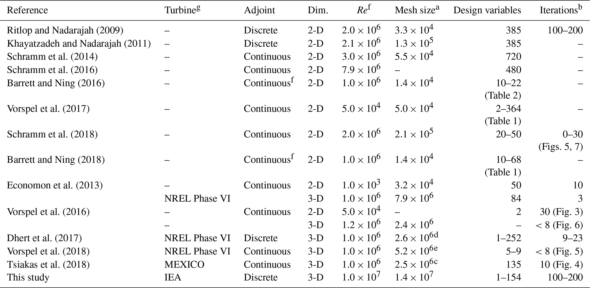
a Number of cells in largest mesh used for optimization. b Not all papers state the number of optimization iterations explicitly. In some cases, we report the number of iterations estimated from the cited figures. As mentioned in Vorspel et al. (2017), this number depends on the optimization problem and optimizer settings, meaning that cross-setup comparison is difficult. c Tsiakas et al. (2018) only gives the number of mesh nodes. d Reduced geometry where the root section was removed. e Applied symmetric boundary conditions (BCs) double the mesh size compared to others. f In cases where a range of Reynolds numbers were used, we report the maximum values. g We only found high-fidelity shape optimization for three turbine configurations in the literature: two smaller turbines – NREL Phase VI and MEXICO (Schepers et al., 2012) – and the large, commercial-scale IEA 10 MW wind turbine. We find it reasonable to assume that the simulations for NREL Phase VI and MEXICO have a Reynolds number on the order of Re=106 (Sørensen et al., 2002, p. 152; Schepers et al., 2012, p. 10), while we estimate the Reynolds number for the IEA turbine to be on the order of Re=107 (Bak et al., 2013, p. 15–16).
Ritlop and Nadarajah (2009) were the first to use a high-fidelity shape optimization method with an adjoint solver for wind turbine profiles. They optimize the lift-to-drag ratio starting from the S809 airfoil using a compressible solver, a low-Mach preconditioner (both for flow and adjoint solver), and the Spalart–Allmaras (SA) turbulence model and find a tendency to increase camber to gain more lift. Finally, they point to the k−ω SST turbulence model and a transition model as needed improvements. Khayatzadeh and Nadarajah (2011) optimized the same airfoil using an enhanced framework that included the cited improvements, where they attempted to postpone the onset of transition. They concluded that both the capability and accuracy of the discrete adjoint optimization framework improved by including the new adjoint variables for the transition model.
There have been several contributions to 2-D RANS shape optimization that use the continuous adjoint approach (Schramm et al., 2014, 2015, 2016, 2018). In these efforts, the continuous adjoint implemented for ducted flows in the flow solver OpenFOAM (Weller et al., 1998) was extended to handle external aerodynamics. First, Schramm et al. (2014) optimized the lift-to-drag ratio of the DU 91-W2-250 profile using 720 design variables while constraining cross-sectional area. They use the “frozen turbulence” assumption, which means that no adjoint equation is used for the turbulence model. Since each surface point in this work is a design variable, they smooth the gradient for stability. The result is a 5.7 % to 59 % increase in lift-to-drag ratio for angles of attack ranging from 6.15 to 9.66∘.
In a later work, Schramm et al. (2015, 2016) presented a finite-difference verification of the adjoint gradients. The same group performed the shape optimization of an upstream leading edge (LE) slat for the DU 91-W2-250 airfoil and a validation of the framework using wind tunnel data, showing good agreement below stall (Schramm et al., 2016). The optimization, which used 480 design variables, resulted in a 2 % decrease in drag. As mentioned previously, there have been other efforts in turbine blade design using 2-D RANS CFD with the adjoint method (Barrett and Ning, 2016, 2018) that used the open-source compressible solver SU2 (Palacios et al., 2013). These works couple the 2-D RANS and adjoint model to BEM, panel, and beam element analysis codes to arrive at a 3-D multi-fidelity and multidisciplinary design framework.
Vorspel et al. (2017) present a benchmark of different optimization algorithms (Nelder–Mead, steepest descent, and quasi-Newton) for unconstrained shape optimization in 2-D, where the continuous adjoint solver within OpenFOAM is used. The benchmark optimization problem is to find a target lift coefficient from any baseline shape. However, they both consider computation time and ease of use to grade the algorithms. As already mentioned, they point to the use of the adjoint method to compute the gradient for a large number of design variables. They recommend that further analysis be done within constrained optimization and within multidisciplinary optimization.
In a more recent work within unconstrained optimization, Schramm et al. (2018) investigated the effect of the “frozen turbulence” assumption in 2-D. They carried out their investigations on the NACA 0012 and DU 93-W-210 airfoils. In this single-point study, they concluded that the implementation of adjoint turbulence models results in better gradients than those obtained through the frozen turbulence assumption. Finally, they specifically mention thickness constraints as a future work topic.
OpenFOAM with a continuous adjoint solver has also been used in 3-D. This was done by Vorspel et al. (2016), who first performed a 2-D test case with two design variables. The 3-D test case consisted of an extruded airfoil with a spanwise length of five chords and a mesh of 2.4×10⁶ cells with an y+ of 2.5. They investigated both a twist and a bend–twist coupling case but found that the bending had no discernible effect. This is something they expect to change for future rotating blades applications.
The above work does not model the rotation, which is important to get the correct local angle of attack along the blade and thus accurately compute the forces acting on the blade. Several 3-D adjoint-based optimization efforts model rotation effects, three of which studied the NREL Phase VI rotor (Economon et al., 2013; Dhert et al., 2017; Vorspel et al., 2018), and another which studied the MEXICO rotor (Tsiakas et al., 2018). Economon et al. (2013) used a continuous adjoint formulation to perform single-point aerodynamic shape optimization using a compressible RANS model. In 2-D, they reduced drag starting from a NACA 4412 profile baseline by 4.86 % under imposed thickness constraints. They used a total of 50 design variables and completed 10 design iterations. In 3-D, they improved the torque coefficient on a mesh with 7.9 million cells by 4 % using 84 shape variables with no constraints imposed on geometry or loads. The free-form deformation (FFD) box covered part of the blade such that both the trailing edge and the innermost part of the blade could not deform.
The optimization was not fully converged, as only three design iterations were performed. One drawback in this early work is the use of the frozen turbulence assumption, which they also identified as an area of future work.
Dhert et al. (2017) used a discrete adjoint solver to carry out a multipoint optimization of a two-bladed rotor using a 2.6 million cell mesh, where they maximized the torque coefficient using up to 252 design variables. They used pitch, twist, and local shape design variables while constraining the thickness between 15 % and 50 % of the local blade chord to ensure adequate space for a structural box. The final multipoint optimization resulted in a 22.1 % increase in torque coefficient but also increased the thrust by 69 %. The original design was meant to be a three-bladed rotor, which explains the low thrust coefficients in the reported results (Dhert et al., 2017, Table 1). They found the optimized shapes for both single and multipoint optimization exhibited highly cambered trailing edges at the root region where the wind speed is reduced. While this does agree with what has been reported in 2-D cases (Ritlop and Nadarajah, 2009), it is also exactly what one would expect when chord is not included as a design variable.
The present work builds on Dhert et al. (2017), who used the same CFD solver, ADflow. Our improvements are summarized in Table 2. One major improvement has to do with the adjoint implementation that was used. As we will explain in more detail later (in Sect. 3.2.2), our adjoint implementation uses the automatic differentiation (AD) technique to compute certain derivatives (Mader et al., 2008). One major improvement is that we implemented the more memory-efficient reverse automatic differentiation. Dhert et al. (2017) was forced to use the less memory-efficient forward automatic differentiation because the reverse option did not include the rotating terms required to model wind turbine rotors. We also added constraints on maximum thrust and flapwise bending moment to align with the IEA case study and enlarged the design space to include chord design variables. Furthermore, Dhert et al. (2017) carried out their studies on the turbine blade excluding the root because of flow solution convergence issues, whereas we include the root. This was made possible by the robustness of the new approximate Newton–Krylov (ANK) solver in ADflow, which also increases its speed (Yildirim et al., 2018). Finally, we achieve an optimality convergence tolerance that is up to 5 orders of magnitude lower.
Dhert et al. (2017)Table 2Overview of differences between the work by Dhert et al. (2017) and the present work.
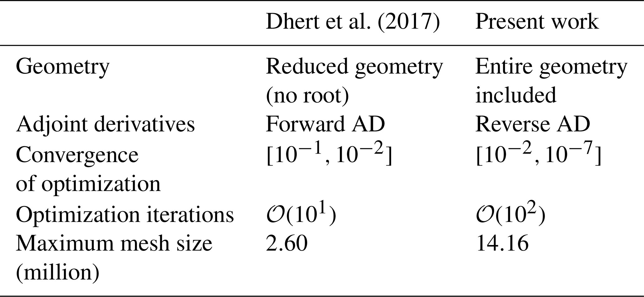
Table 3Overview of aerodynamic optimization works of wind turbine rotors using the adjoint method.

Multi: multipoint optimization; turbulence: whether the turbulence model is included in the adjoint solver; deformation: whether the entire blade was allowed to deform; geometry: whether the entire blade was modeled; geometric constraints: whether any geometric constraints were imposed.
Another recent effort is that of Vorspel et al. (2018), who performed unconstrained optimization of the NREL Phase VI rotor where they minimized the thrust by varying up to nine twist design variables using a steepest descent optimization algorithm. Not surprisingly, they mention convergence issues, in part due to the turbine being stall regulated and exhibiting separated flow at some inflow speeds. Vortices at tip and root further impaired the convergence, which in turn resulted in poor gradient quality. They addressed this issue by limiting the deformable area to only the outer 50 % of the blade length, which limited the shape design optimization. Like Economon et al. (2013), they used the frozen turbulence assumption. However, they differed in choice of turbulence model: Vorspel et al. (2018) used the k−ω SST model, while Economon et al. (2013) used the SA turbulence model. For future work, they suggested the use of more efficient optimization algorithms, and mentioned the inclusion of the adjoint turbulence equations and the study of turbines that are not stall regulated.
Finally, Tsiakas et al. (2018) used a continuous adjoint approach that included the SA turbulence equations to optimize the MEXICO RWT. The flow was modeled by the incompressible RANS equations and solved in a co-moving frame of reference. They maximized the power for a single wind speed of 10 m s−1. Compared to the present work, they used a different parameterization technique based on volumetric non-uniform rational B splines (NURBS), which confine the blade in a small volume. NURBS are used both for the deformation of the surface and the volume meshes, and the outermost NURBS control points are fixed to keep the outer volume mesh fixed. This only ensures C0 continuity. They use 385 NURBS, resulting in 135 design variables, which are only allowed to move in the direction perpendicular to the rotor plane. This choice of parameterization limits the design space; for example, no chord increase can be obtained without simultaneously changing profile shape. The flow and adjoint solvers take advantage of graphics processing unit (GPU) hardware, resulting in fast solutions. Indeed, they state that the overall optimization process can run up to 50 times faster on GPUs than on CPUs. They obtained a 3 % increase in the objective function and attribute this modest improvement to the limited freedom in the parameterization.
In spite of the contributions cited above, many improvements are needed before we achieve the ultimate goal of providing a “push-button solution” for wind turbine manufacturers. This paper contributes with some of these improvements by including all of the following features in a comprehensive high-fidelity 3-D RANS-based shape optimization framework:
-
enforcement of geometric constraints to ensure structural feasibility,
-
normal operation rotor load constraints limiting thrust and flapwise bending moment,
-
more precision and stability in the convergence of flow and adjoint solvers,
-
inclusion of a turbulence model in the adjoint solver,
-
a comprehensive set of design variables, and
-
modeling and deformation of the entire blade shape.
In Table 3, the present work is compared to the above-cited 3-D shape optimization efforts on wind turbine rotors.
As previously mentioned, structural considerations are crucial in wind turbine design. Anderson et al. (2018) partially addressed this issue by coupling the NSU3D RANS solver with the AStrO structural finite element solver through a fluid–structure interface to converge on realistic, steady-state loads on the SWiFT RWT. They used Abaqus to make a finite element model with shell elements. They performed a purely structural optimization of the composite blade, with the loads computed by the CFD. The optimization's objective was to, using gradient-based optimization, minimize the off-axis stress with respect to 16 310 ply orientation variables. They completed 10 optimization iterations considering five different load cases and achieved a reduction in the maximum fatigue stress between 40 % and 60 %. They did so without adding any constraints, but they did assume the material to be a single-ply, unidirectional fiber composite for each blade section. The logical next step would be to perform the simultaneous optimization of the structural sizing and aerodynamic shape optimization, as is already done in aircraft wing design (Kenway and Martins, 2014).
We now briefly describe all components of the optimization framework. The overall workflow is shown in Fig. 1 using an extended design structure matrix (XDSM) diagram (Lambe and Martins, 2012). An initial set of design variable values, x(0), is given to the optimizer. The optimizer passes the current design variables to the surface deformation module, prompting it to update the surface mesh (except for the very first iteration). The surface deformation module also provides analytic derivatives of the surface mesh with respect to the design variables, dxs∕dx. After the surface mesh has been updated, it is passed to the volume deformation module, which updates the volume mesh and computes its analytic derivatives with respect to the surface mesh, dxv∕dxs. Then, the flow solver computes the flow states, w. These states are passed to the adjoint solver, which computes the total derivative. Finally, the objective function, f (e.g., torque), as well as its derivatives, df∕dx, are provided to the optimizer, which computes a new step for another optimization iteration. Both the surface and volume deformation steps are fast explicit operations. On the other hand, the flow and adjoint solvers are costly iterative operations that take up the vast majority of the computation time. The optimization process involves 𝒪(102) major iterations, which is an absolute minimum bound on the number of CFD solutions and mesh updates; there are additional CFD solutions within each major iteration.
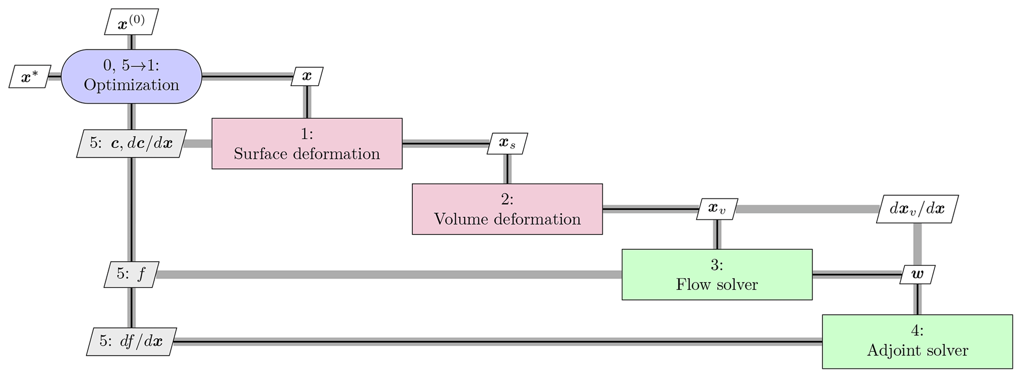
Figure 1Extended design structure matrix (XDSM) showing the optimization framework. Green blocks are iterative solvers, whereas red boxes represent explicit functions. Black lines represent the process flow in the order of the numbers; gray lines represent data dependencies.
3.1 Geometry and mesh deformation
To deform the surface geometry and mesh, we use the Python module pyGeo developed by Kenway et al. (2010), which implements the FFD (Sederberg and Parry, 1986) technique. Some of the key features of FFD are analytic derivatives and a machine-precision representation of the baseline geometry.
The volume deformation tool is called IDWarp and is based on the inverse distance weighting function (Edward et al., 2012). IDWarp is a fast and unstructured deformation algorithm that has been demonstrated in aerodynamic (Yu et al., 2018; He et al., 2018) and aerostructural applications (Brooks et al., 2018).
3.2 Flow and adjoint solvers
3.2.1 EllipSys3D
EllipSys3D is an in-house, structured, multi-block, finite volume method (FVM) flow solver developed at DTU Wind Energy by Michelsen (1992, 1994) and Sørensen (1995), and we use it in the present work to perform the comparison between CFD solvers. It discretizes the incompressible RANS equations using general curvilinear coordinates and couples velocity and pressure through the SIMPLE algorithm.
In this study, we run EllipSys3D using the third-order quadratic upwind interpolation for convection kinematics (QUICK) scheme and the k−ω SST (Menter, 1993) model to calculate the turbulent eddy viscosity, which compares favorably to other turbulence models for wind turbine applications (Reggio et al., 2011).
EllipSys3D has been validated against experimental data for the MEXICO RWT (Bechmann et al., 2011) and the NREL Phase VI RWT (Sørensen et al., 2002; Sørensen and Schreck, 2014), and also in a blind comparison (Simms et al., 2001). In addition, the unsteady interaction between tower and blade has been simulated for the NREL Phase VI RWT with EllipSys3D using overset grid capabilities, and an overall good agreement was found with experimental data (Zahle et al., 2009). EllipSys3D has been used in various rotor applications to perform computations, such as aerodynamic power (Johansen et al., 2009) and fluid–structure interaction (Heinz et al., 2016). The latter work also encompasses a comparison across fidelities between the CFD-based tool, HAWC2CFD, and the BEM-based HAWC2 solvers where a good agreement was found. EllipSys3D has also been compared with OpenFOAM for a case with atmospheric flow over complex terrain. EllipSys3D was found to be 2–6 times faster while producing almost identical numerical results (Cavar et al., 2016). More recent sources also show that these two solvers yield comparable results (Sørensen et al., 2016; Yilmaz et al., 2017; Boorsma et al., 2018).
3.2.2 ADflow
ADflow is a compressible RANS solver based on SUmb (Weide et al., 2006), a structured FVM CFD solver written in Fortran 90 that uses cell-centered variables on a multi-block grid. Unlike EllipSys3D, ADflow uses the Spalart–Allmaras (SA) turbulence model (Spalart and Allmaras, 1994) and works with state variables computed using the Jameson–Schmidt–Turkel (JST) scheme. More recently, Kenway et al. (2017) implemented overset mesh capability. ADflow is wrapped with Python to provide a more convenient user interface and to facilitate integration with optimization algorithms and other components of an MDO framework.
ADflow has been coupled to a structural finite element solver in the MACH (MDO for aircraft configurations with high fidelity) framework (Kenway et al., 2014), which has been used to perform not only aerostructural optimization of aircraft configurations (Kenway and Martins, 2014; Brooks et al., 2018; Burdette and Martins, 2018, 2019) but also hydrostructural optimization of hydrofoils (Garg et al., 2019, 2017).
As previously mentioned, we use an ANK solver, which is implemented in ADflow to provide robustness. The ANK implementation is important since it is crucial to properly converge the flow field in order to obtain accurate gradients. Newton–Krylov (NK) methods are not robust because they might not converge if the starting point is outside the basin of attraction. ANK addresses this convergence issue using a globalization method called pseudo-transient continuation, which starts with the stable but inefficient backward Euler method with a small time step, and then increases the time step to approach the higher convergence rate of the NK solver. The ANK method involves the solution of large linear systems using preconditioners. These systems are solved in a matrix-free fashion with the generalized minimal residual (GMRES) algorithm (Saad and Schultz, 1986) using the Portable, Extensible Toolkit for Scientific Computation (PETSc) library (Balay et al., 2018a, b, 1997). The adjoint solver linear systems are solved using the same algorithm. ADflow is considered converged when the ratio of the L2 norm of the residuals at iteration n and the same norm of the free stream residual is below a given tolerance, i.e., when
For the optimizations presented below, we typically set , whereas the L2 convergence for the adjoint equation is set to 10−7. These convergence thresholds are not to be confused with the optimality tolerance, which we set to 10−4.
One crucial capability in ADflow is the efficient computation of gradients through its adjoint solver. Together with the geometry and mesh deformation tools mentioned above, and the optimization software mentioned in the next section, this enables aerodynamic shape optimization with respect to hundreds of design variables (Lyu et al., 2014; Chen et al., 2016; Dhert et al., 2017). All the optimization results in Sect. 6 are obtained with the ADflow framework.
We now derive the adjoint equations and briefly explain how they are assembled and solved. A detailed description of the implementation is provided in previous work (Mader et al., 2008; Mader and Martins, 2011; Lyu et al., 2013). The CFD solver computes the flow field, w, for a given set of design variables, x, by converging the residuals R(x,w) of the governing equations to zero. Then, any function of interest, f(x,w), can be computed. Gradient-based optimizers require the gradient of the objective and constraint functions with respect to the design variables. To compute this gradient, we use the equation for the total derivative:
Here, the partial derivatives correspond to derivatives of explicit functions, while the total derivative involves the iterative solution of the governing equations. Thus, the partial derivatives can be found analytically at a low computational cost, but the direct computation of the total derivative dw∕dx should be avoided. A similar total derivative equation can be written for the residuals, which must remain zero for the CFD solution to hold, and thus
We can now substitute the solution of the Jacobian given by the above equation into the total derivative equation (Eq. 2) to obtain
where we have only partial derivative terms that can be found analytically at a low computational cost. The linear system in this equation can either be solved by computing the solution Jacobian, dw∕dx, from the linear system from Eq. (3) or by solving the adjoint system:
where Ψ is the adjoint vector, which can be substituted into the total derivative equation (Eq. 2), i.e.,
The cost of the adjoint method is independent of the number of design variables because the adjoint equation (Eq. 5) does not contain x. However, if there are multiple functions of interest f, we need to solve Eq. (5) for each f with a different right-hand side. Given that our problem has 𝒪(102) design variables and only a few functions of interest, the adjoint method is particularly advantageous.
In the adjoint equation (Eq. 5) and total derivative equation (Eq. 6), we need to provide two matrices and two vectors of partial derivatives. As mentioned above, these derivatives involve only explicit operations and are in principle cheap to compute. However, they still require the differentiation of parts of a complex CFD code, and a good implementation is essential to preserve the accuracy and efficiency of the adjoint approach. Traditionally, adjoint method developers have derived these partial derivatives by differentiating the equations or code manually and programming new functions that compute those derivatives. This process is labor intensive and prone to programming errors. To address this drawback, Mader et al. (2008) pioneered the use of automatic differentiation to compute the partial derivatives. Automatic differentiation is a technique that takes a given code and produces new code that computes the derivatives of the outputs with respect to the inputs (Griewank, 2000). Using a pure automatic differentiation approach to compute our derivatives of interest, df∕dx, would mean applying the automatic differentiation tool to the whole CFD code, including the iterative solver. While this produces accurate derivatives, it is not an efficient approach. By selectively using automatic differentiation to produce code that computes only the partial derivatives, which do not involve the iterative solver, we lower the adjoint implementation effort while keeping the efficiency of the traditional adjoint implementation approach. There are still many details involved in making our adjoint implementation approach efficient; these details have been presented in previous work (Mader et al., 2008; Lyu et al., 2013).
As briefly mentioned in the introduction, there are two modes for automatic differentiation: the forward mode and the reverse mode. Dhert et al. (2017) had used automatic differentiation in forward mode to compute and store the flow Jacobian, , as well as the other partial derivatives. Then, these stored matrices are used by the adjoint solver to compute transpose-matrix-vector products to converge the adjoint solution, Ψ. Using the reverse mode, no storage of the Jacobian is needed. Instead, a matrix-free approach is used, where the transpose-matrix-vector products required to converge the adjoint solution are computed directly through the reverse mode derivative routines. While the reverse mode is more efficient in terms of memory usage, the reverse mode implementation was missing the rotation terms required for wind turbine modeling. We have fixed this for the implementation in the present work and use the reverse mode instead. The implemented reverse AD routines may also lead to speed up depending on the number of Krylov iterations needed to converge the adjoint system.
3.3 Optimizer
We use the Sparse Nonlinear OPTimizer (SNOPT) (Gill et al., 2002) for all optimizations herein. SNOPT implements a sequential quadratic programming (SQP) algorithm. We use it through the open-source Python wrapper pyOptSparse4, which provides a common interface to this and other optimization software. The convergence in SNOPT is set through the “major optimality tolerance” setting (Gill et al., 2007). We aim at converging all optimization problems to 10−4.
In this work, we use ADflow as the CFD solver in the design optimization due to its adjoint gradient computation and integration with geometry parameterization, mesh deformation, and optimization tools. However, EllipSys3D has been more thoroughly validated for wind turbine rotor flows, so in this section, we verify ADflow against EllipSys3D for a three-bladed pitch-regulated rotor geometry. In this section, we only include a mesh convergence study for one operational condition. A more detailed flow comparison is included in Appendix Appendix A.
4.1 Fluid model and computational mesh
All simulations are steady-state 3-D RANS of the rotor only, where effects from both tower and nacelle have been neglected. Since we study a rigid upwind turbine, neglecting tower and nacelle should have a limited effect. We also note that we compute the flow field using a co-rotating, non-inertial reference frame that is attached to the rotor. Therefore, the RANS equations have additional terms to account for Coriolis and centripetal forces. Just as for the IEA Wind Task 37 case, the three-bladed pitch-regulated rotor geometry in the analysis is a design based on the DTU 10 MW RWT (Bak et al., 2013), where both chord and twist distributions have been altered to allow for more room for improvement using design optimization. We compare the twist and thickness distributions for the DTU 10 MW RWT and the IEA Wind Task 37 baseline in Fig. 2
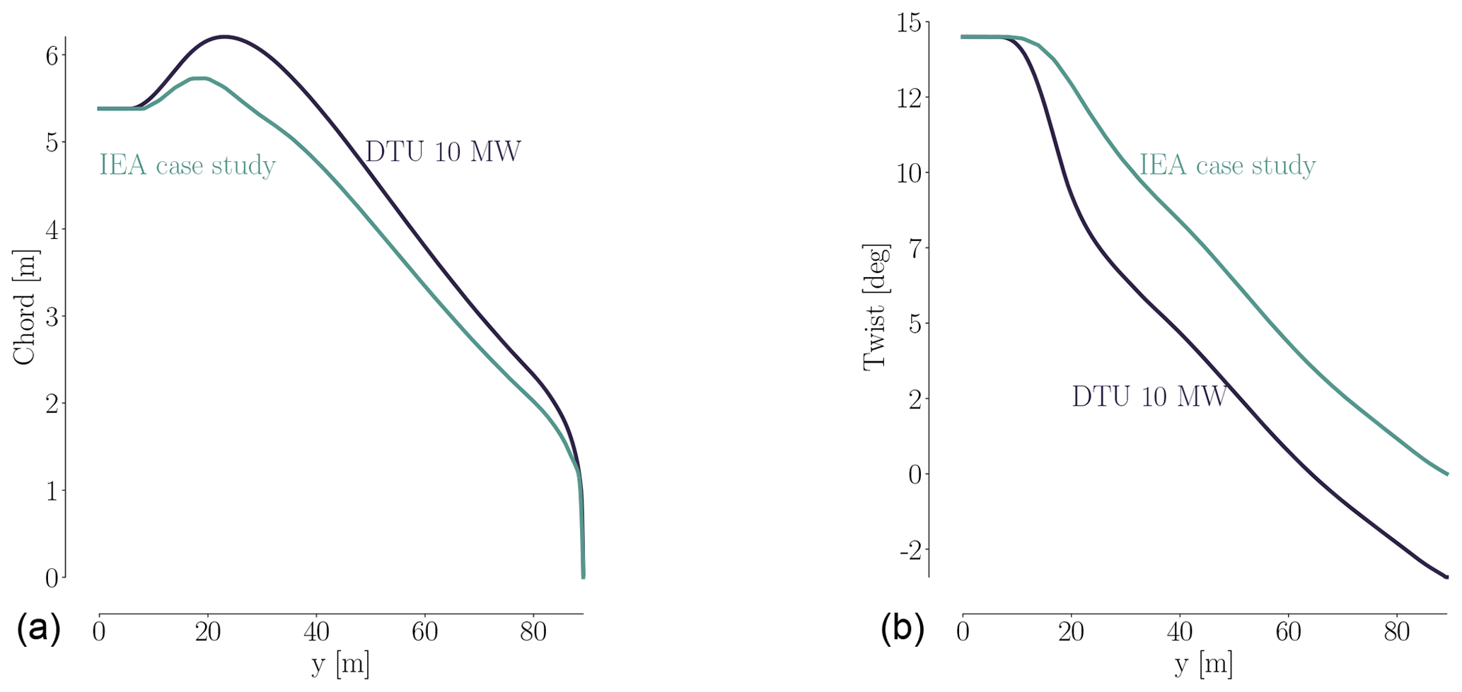
Figure 2Comparison of chord (a) and twist (b) for the DTU 10 MW RWT and the perturbed design used as the starting point for the IEA optimization case study. Both the chord and twist are reduced. The baseline blade design is based on the FFA-W3 airfoil family with relative thicknesses in the range of [24 %,36 %].
The surface mesh consists of three blades, each with 36 blocks. For each blade, there are 256 cells in the chordwise direction and 128 in the spanwise direction (tip excluded). The surface mesh is generated using the in-house Parametric Geometry Library (PGL). The tip was constructed using four blocks of 32×32 cells each, resulting in a total surface mesh with 110 592 mesh cells.
The spherical volume mesh has an O–O topology generated with the hyperbolic in-house mesh generator HypGrid (Sørensen, 1998). Setting the first boundary layer cell height to 10−6 m yields a y+ of around 1 for the given operational conditions, and a total of 128 cell layers are grown from the surface mesh where the farthest vertices reach a distance of 1740 m. This results in a total of 432 blocks, each with cells, which is equivalent to 14.155776 million cells. Given a span of R=89.166 m, the surrounding spherical mesh expands to about 20 times the blade span.
The mesh we just described above is the finest mesh we use, which we call the L0 mesh. A coarser (L1) mesh is obtained by coarsening L0 once, i.e., by removing every second cell in all three directions. Similarly, the L2 mesh is obtained by coarsening L1. Unless otherwise stated, we use these three meshes in all the work herein. The turbine geometry and the surrounding spherical mesh are shown in Fig. 3, and a more detailed view of the rotor is shown in Fig. 4.
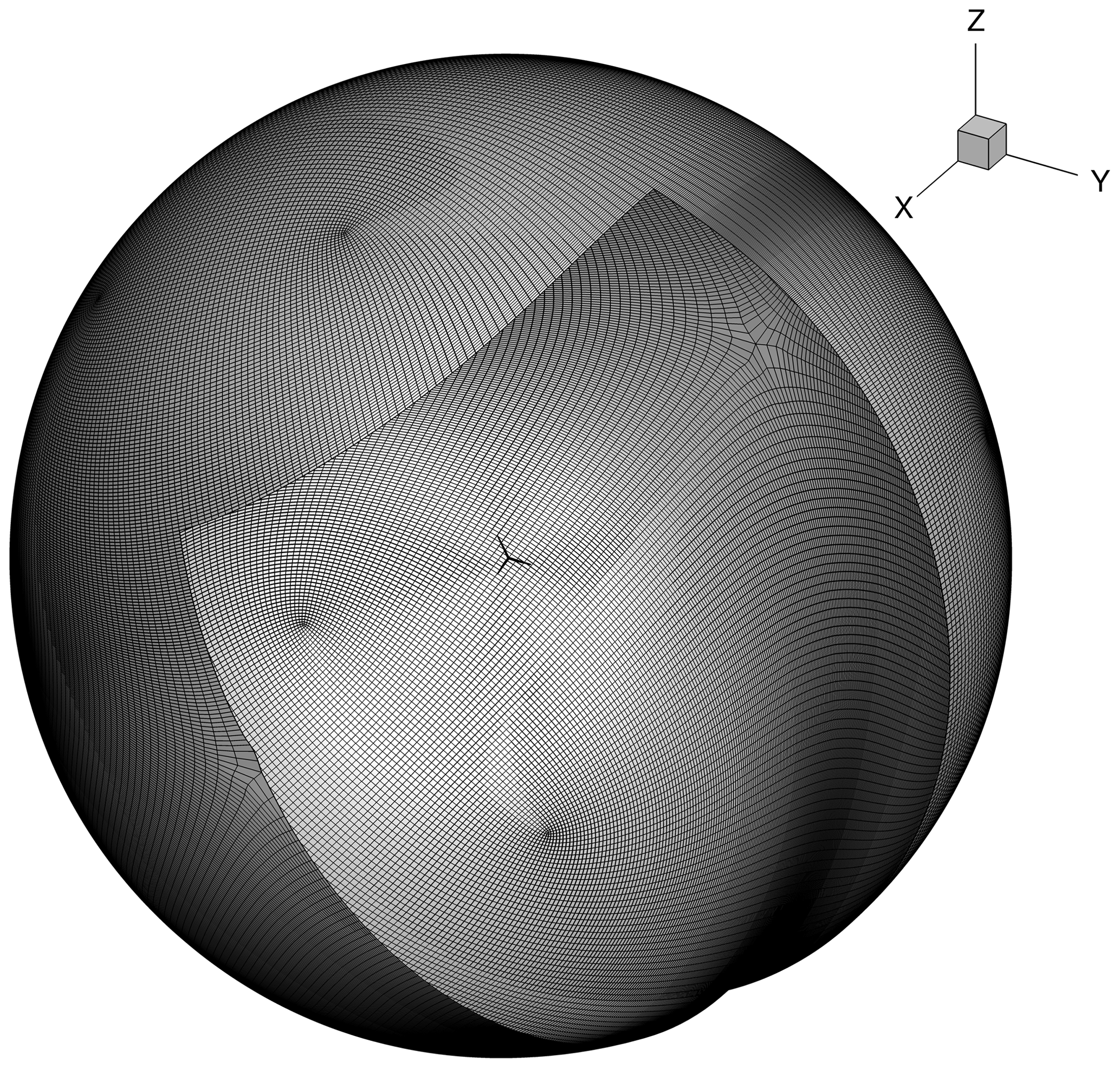
Figure 3The baseline wind turbine design with the spherical L0 mesh around it. The blade span is 89.166 m, and the spherical mesh stretches to 20 times the blade span.
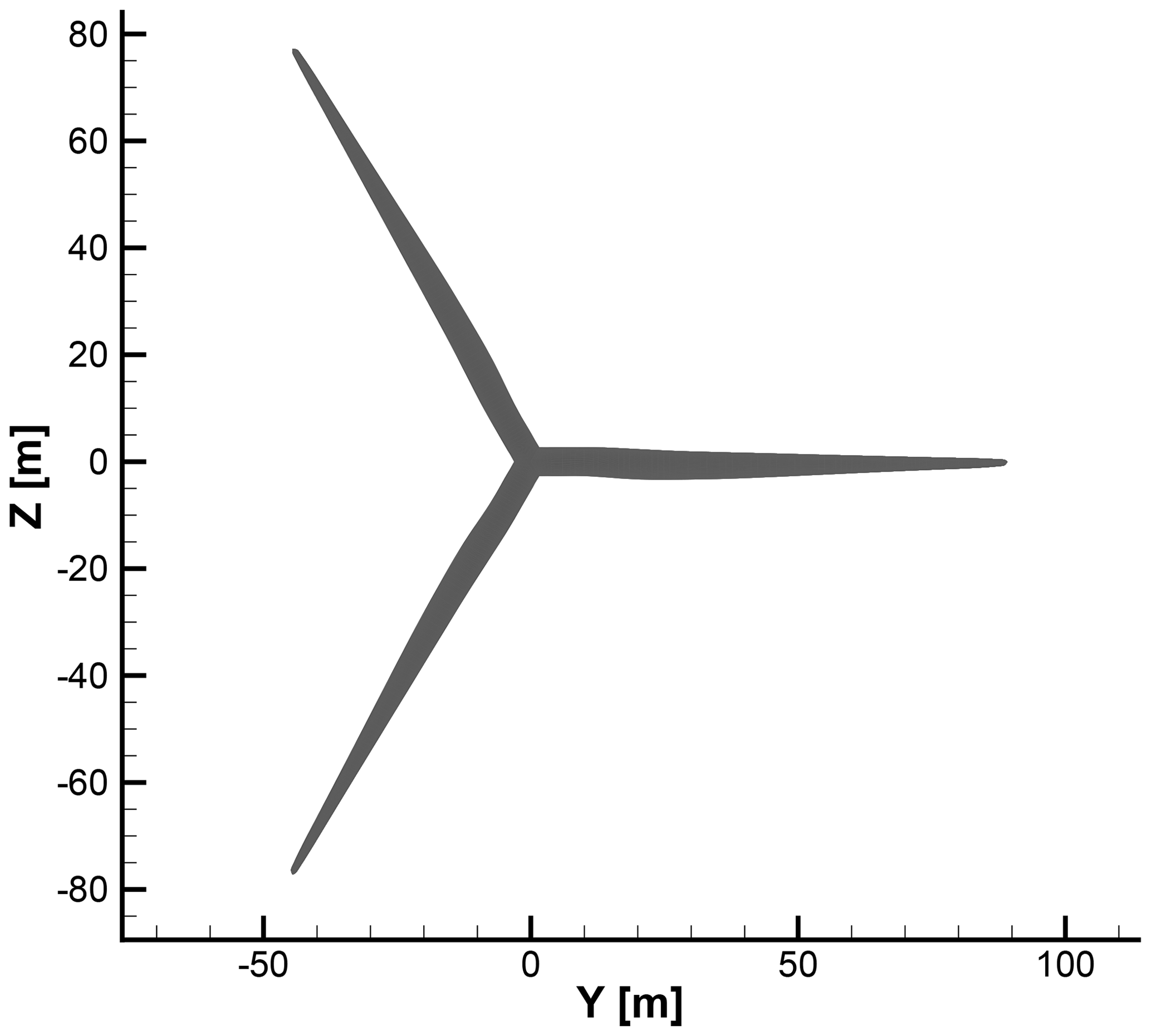
Figure 4Baseline geometry used in the flow solver comparison and as starting point for the optimization. Each blade has a surface mesh with 36 square blocks. Each block has 32×32 cells, resulting in 110 592 surface mesh cells.

4.2 Mesh convergence study
To quantify the mesh dependence for each solver, we compute the integrated metrics – torque and thrust – for the three mesh levels (L0, L1, and L2) and list them in Table 4. The operational condition corresponds to a wind speed of 8 m s−1 and rotor speed of 6.69 rpm at zero blade pitch, which is one of the conditions listed in Table A1 in Appendix Appendix A. As is evident from the results for meshes L2, L1, and L0 in Table 4, ADflow does not produce a sufficiently mesh-independent solution on mesh L0. This agrees with an earlier mesh convergence study (Dhert et al., 2017, Table 1), where up to 22 million cells were used without reaching convergence. Therefore, we generated a finer mesh with more than 47 million cells called L-1. The L-1 mesh is made exclusively for the present grid convergence study and will not be used in the ensuing optimizations.
Table 4Mesh convergence study for the compressible solver ADflow and the incompressible solver EllipSys3D. The operational conditions for the convergence study correspond to the 8 m s−1 case listed in Table A1. The error percentages are estimated using the Richardson extrapolations from Fig. 5.
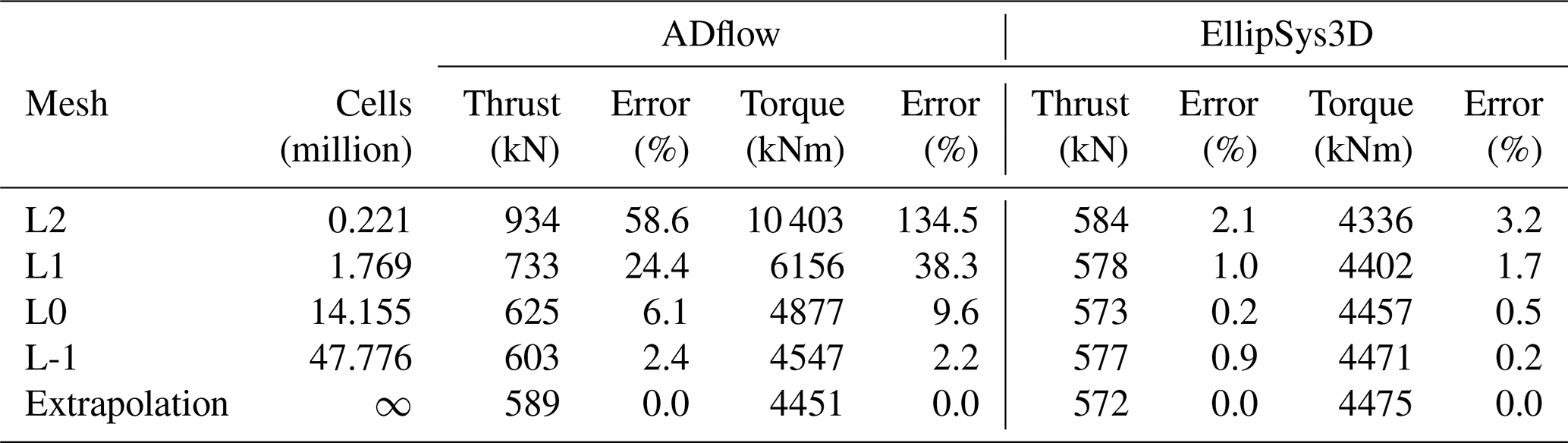
Table 4 shows that error reduction from L0 to L-1 for ADflow is much lower (with reductions of about 4 % in thrust and 7 % in torque) than the error reduction from L2 to L1 (15 % and 21 %) or from L1 to L0 (22 % and 41 %). The errors are computed using the Richardson extrapolation values from Fig. 5, which are based on an estimate of the continuum value (in the limit of an infinitely fine mesh), given by Roache (1994):
where fc is the continuum value, f1 and f2 are the values obtained using the L0 and L1 meshes, respectively, and r is the grid refinement ratio.
In Table 4, we can also see that the two solvers tend to converge towards the same thrust and torque continuum values – 0.3 % difference for thrust and 0.7 % difference for torque. Based on the results in this table, we determine that the L0 mesh represents a reasonable compromise between accuracy (less than 10 % error) and speed.
It is clear from Fig. 5 that mesh level L2 is very coarse and yields very different results. As we will demonstrate later, the suggested design trends from such a coarse mesh can sometimes lead to savings in computation time and, other times, lead to completely wrong design trends. Thus, one should use such coarse meshes with care. We report the results obtained with L2 throughout the presented work to substantiate this claim.
There is a slight increase in error for EllipSys3D in the thrust value on the finest mesh level, which is unexpected. It is also surprising that the compressible solver seems to benefit so drastically from an increase in cell count. Recent studies have suggested this can be the case for some compressible solvers (Sørensen et al., 2016). From the expressions for the Prandtl–Glauert compressibility corrections (Glauert, 1928), one would expect that compressible effects could be at play, which agrees with our results. Compressibility effects in wind turbine applications have become increasingly significant as turbine rotor sizes have increased. One of the conclusions from the AVATAR project was that compressibility effects play a role in large wind turbines (Sørensen et al., 2017, p. 9). In the AVATAR project, results from EllipSys3D were compared to results from a compressible CFD code. Here, they studied a case with an inflow speed of 14 m s−1 and a Mach number of 0.2457 (Sørensen et al., 2017, Fig. 8), where the obtained Cp curves differed in particular on the suction side close to the trailing edge (TE). The resulting sectional forces on the blade differed up to 12.9 % (Sørensen et al., 2017, Table 3). The cited Mach number of 0.2457 is within the Mach number range of the present work, where we have Mach numbers close to 0.3 at the tip depending on the inflow speed. The effects of compressibility near the tip region have recently been studied by Sørensen et al. (2018). This work also includes results obtained with EllipSys3D. They find that classical compressibility corrections to incompressible results can be applied in a post-processing step in order to reduce the lift and drag error to within 2.5 % for Mach numbers up to 0.3. The cases studied by Sørensen et al. (2018) include Mach numbers ranging from 0 to 0.5.
This suggests that we could hope to further align the results between ADflow and EllipSys3D in future work by using classical compressibility corrections. Based on the grid convergence study above and in Appendix Appendix A, where we provide more details on the flow phenomena and solver performance, we conclude that while there are discrepancies due to different turbulence models, compressibility effects, and numerical scheme order, the trends for the two solvers largely agree.
In this section, we first introduce the design optimization problems for all the CFD and BEM cases we solve. We then explain the FFD parameterization, geometric constraints, and rotor load constraints.
5.1 Design optimization problem
We adapt and extend the design optimization problem from the IEA Wind Task 37 case study, which is to maximize the AEP for a range of wind speeds by varying chord and twist, while constraining the increase in thrust and bending moment to be no more than 14 % and 11 %, respectively. Thickness constraints are enforced over the blade to ensure structural integrity. Mathematically, the IEA Wind Task 37 design optimization problem can be expressed as follows:
The AEP is computed using a specified Weibull distribution (with scale and shape parameters A=8 and k=2, respectively) and the power produced for each wind speed, which is computed from the torque, Q, produced by the turbine ().
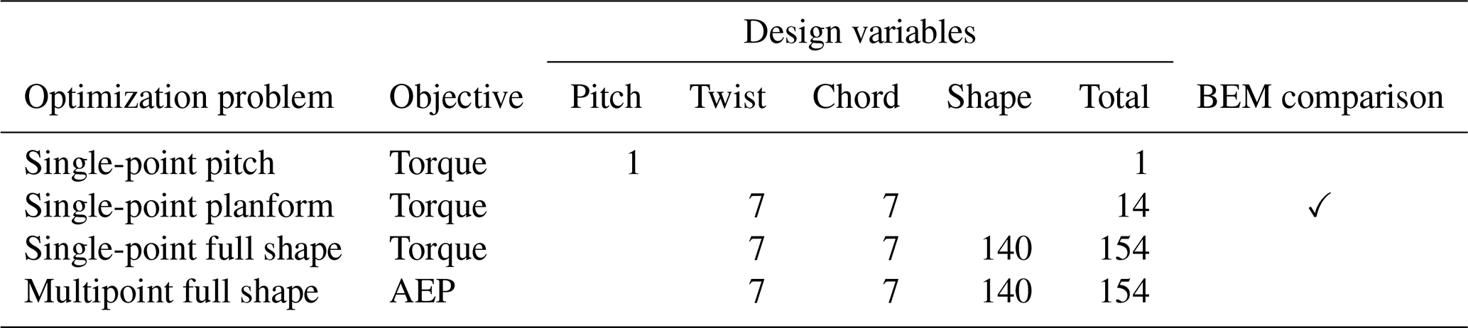
We solve four different CFD-based optimizations derived from the problem above:
- Single-point pitch optimization:
-
This is used to maximize torque on the turbine with respect to blade pitch for a single wind speed (which in this case is equivalent to maximizing AEP). The purpose of this case is to validate the newly implemented rotational terms in the adjoint solver.
- Single-point planform optimization:
-
This is the same as the IEA Wind Task 37 problem (Eq. 8), except with the objective of maximizing torque for a single wind speed. We solve this problem because it is well suited for comparison with BEM.
- Single-point full shape optimization:
-
This is the same as the single-point planform optimization but with the addition of blade shape variables. This problem takes advantage of the additional design freedom that is not available for BEM-based models.
- Multipoint full shape optimization:
-
This is the same as the IEA Wind Task 37 problem (Eq. 8) but with the addition of blade shape variables.
The single-point optimizations are all performed for a wind speed of 8 m s−1 and rotational rate of 6.69 rpm at zero blade pitch, which is one of the conditions listed in Table A1 in Appendix Appendix A. For the multipoint optimizations, we use the wind speeds 5, 8, and 11 m s−1, and the relevant operational conditions can again be found in Table A1 in Appendix Appendix A. Furthermore, we use the initial values at 12 m s−1 in the thrust and flapwise bending moment constraint for the multipoint optimizations because we know from the solver comparison (Appendix Appendix A, Fig. A1) that the maximum thrust occurs at that speed.
In addition to the CFD-based optimizations, we solve two BEM-based optimization problems for comparison with the CFD-based planform optimization:
- BEM1:
-
identical to the single-point planform optimization.
- BEM2:
-
identical to the multipoint full shape optimization, except the shape variables are replaced by spanwise thickness distribution variables.
The thickness is handled by interpolating between the predefined airfoil data. While both BEM1 and BEM2 use specified airfoil polar data, BEM2 can change the relative thickness of the airfoils. The airfoils vary from 72 % to 24 % in relative thickness.

Figure 6Overview of baseline geometry and FFD boxes (a). Each FFD box has nine spanwise sections. Each blade (b) has 15 thickness constraints (blue) and seven LE/TE constraints (red). Thickness distributions (c) are for the baseline thickness (green) and minimum allowed thickness (purple). Profile section (d) at 36 m span shows the shape control points (20), the thickness constraints (10 blue segments) and LE/TE constraints (two red segments). The LE/TE constraints are only relevant for the full shape optimizations.
5.2 Parameterization
The baseline design is shown in Fig. 6a, along with the three FFD boxes used to parameterize the geometry. The FFD boxes have control points (shown in black), where 10 is the number of control points from LE to TE, 9 is the number of spanwise sections, and 2 corresponds to the top and bottom of the FFD box. Our approach to deciding on the number of control points is to use the largest number possible to provide maximum freedom in the optimization. However, as the density of control points approaches that of the CFD mesh, numerical issues occur because the physical model no longer resolves the effect of the geometry change. We have found that, as a rule of thumb, we should have no more than one control point for every four CFD mesh points.
The FFD boxes are used to apply the pitch, twist, chord, and shape variables to each blade. Since we want all three blades to have the same pitch and shape, the variables are forced to be the same. Furthermore, the FFD boxes have two fixed sections close to each other at the root to ensure C1 continuity there, while the seven outer sections are free to move and deform the blades. Pitch, xpitch, is achieved by rotating all free FFD sections by the same amount along the reference axis, which is at 35 % of the chord from the LE. Twist, xtwist, is achieved by rotating each spanwise section of FFD control points independently. The chord variables, xchord, are achieved by scaling each spanwise section in the chord and thickness direction. Thus, the relative thickness at each section is preserved during the CFD planform optimization. Only for the full shape optimizations, where the shape variables are added, can the relative thickness change. The shape variables, xshape, move each control point independently in the direction perpendicular to the chord to control the airfoil shape.
In Fig. 6, the thickness constraints are highlighted in blue. The thickness constraints in the BEM comparison are only enforced on the inner 80 % of the blade, as detailed in the definition of the IEA case study. This is also visualized in Fig. 6c.
There were a few necessary changes we made to the IEA case study, but only for the full shape optimizations. One such deviation is the dashed segment connected to the thickness limit curve in Fig. 6, which prevents negative cell volumes. Furthermore, there are constraints applied to the LE and TE of the FFD box. The LE/TE constraints (shown in red in Fig. 6) are only implemented for the single-point and multipoint full shape optimizations. These constraints force each pair of points to move exactly the same amount in opposite directions, so that the midpoint in the segment remains stationary. This ensures that the individual FFD control points do not apply skewing twist, since they are meant to control only airfoil profiles. Finally, we mention that the thickness limit is fully imposed only for the fourth thickness constraint (counting from the LE), while the remaining nine constraints in a section are relaxed to not unnecessarily restrict the possible design space.
The results are split into the four main problems listed in Table 5. First, we perform a single design variable optimization where pitch is varied to maximize the torque (Sect. 6.1). This simple optimization is included to validate the adjoint formulation for rotating frame of reference flows. Second, we perform a planform optimization where chord and twist are varied (Sect. 6.2). This optimization is well suited for comparison with BEM results because the airfoil shapes do not change. The two final optimizations are full shape optimization problems where all variables, including airfoil shape variables, are allowed to change. First, we solve the problem as a single-point optimization (Sect. 6.3). Then, we solve it as a multipoint optimization (Sect. 6.4).
6.1 Pitch optimization
In the pitch optimization, the pitch angle for the seven outer FFD sections on each blade is controlled by a single design variable. The optimization result is an increase in torque of 25.7 %, 26.1 %, and 23.0 % for mesh levels L2, L1, and L0, respectively. Figures 7–9 summarize the optimization history for the three mesh levels.
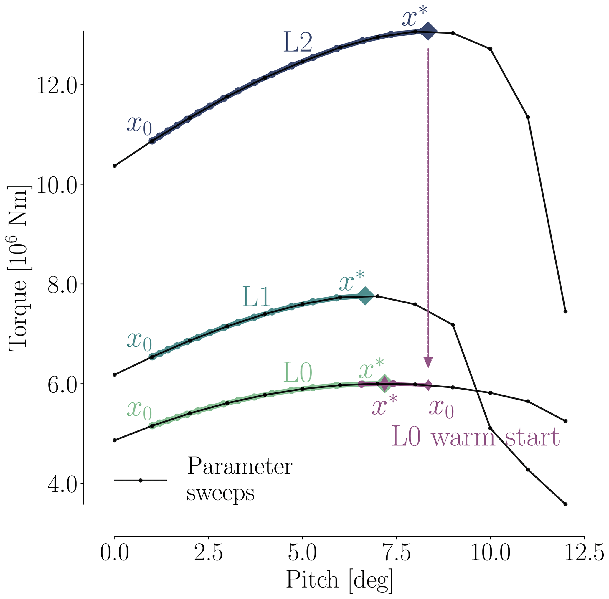
Figure 7 shows the torque as a function of pitch. Before optimizing, we performed a sweep of CFD evaluations of the torque for the whole range of pitch values, for all three mesh levels. These are represented by black dots in Fig. 7. The thin black lines are linearly interpolated from these points. Although the torque value varies between mesh levels, the trends are consistent, and the maximum torque is achieved around 7∘ of pitch. The optimization histories for each mesh are shown in color; they start from the initial pitch, x0, and end at the optimal one, x*. The purple line shows the optimization history on the finest (L0) mesh that was obtained by using the result from a coarser mesh (L2) as a starting point. We use this “warm start” technique since coarser meshes are much faster to converge. This technique leads to a reduction of computation time since fewer steps are taken by the optimizer on the finest mesh level. This is seen in Table 6, where only four steps were needed instead of the 16 steps taken in the original optimization. In this case, it reduced the computation time at approximately 50 %. As expected, the result of this warm start optimization is identical to the result of optimizing solely on the finest mesh level. Now that we have introduced (and visualized in Fig. 7) the use of warm starts, we will start using them regularly. This means that an L1 optimization from now on uses the result of an L2 optimization, and an L0 optimization uses the result of an L1 optimization.
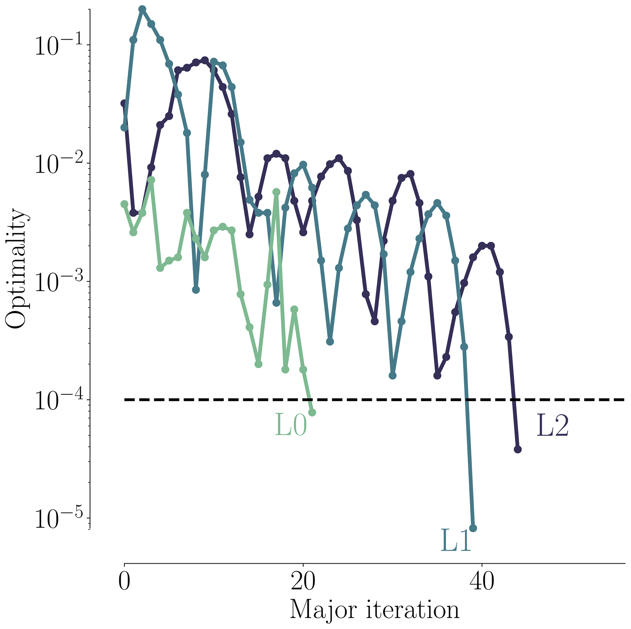
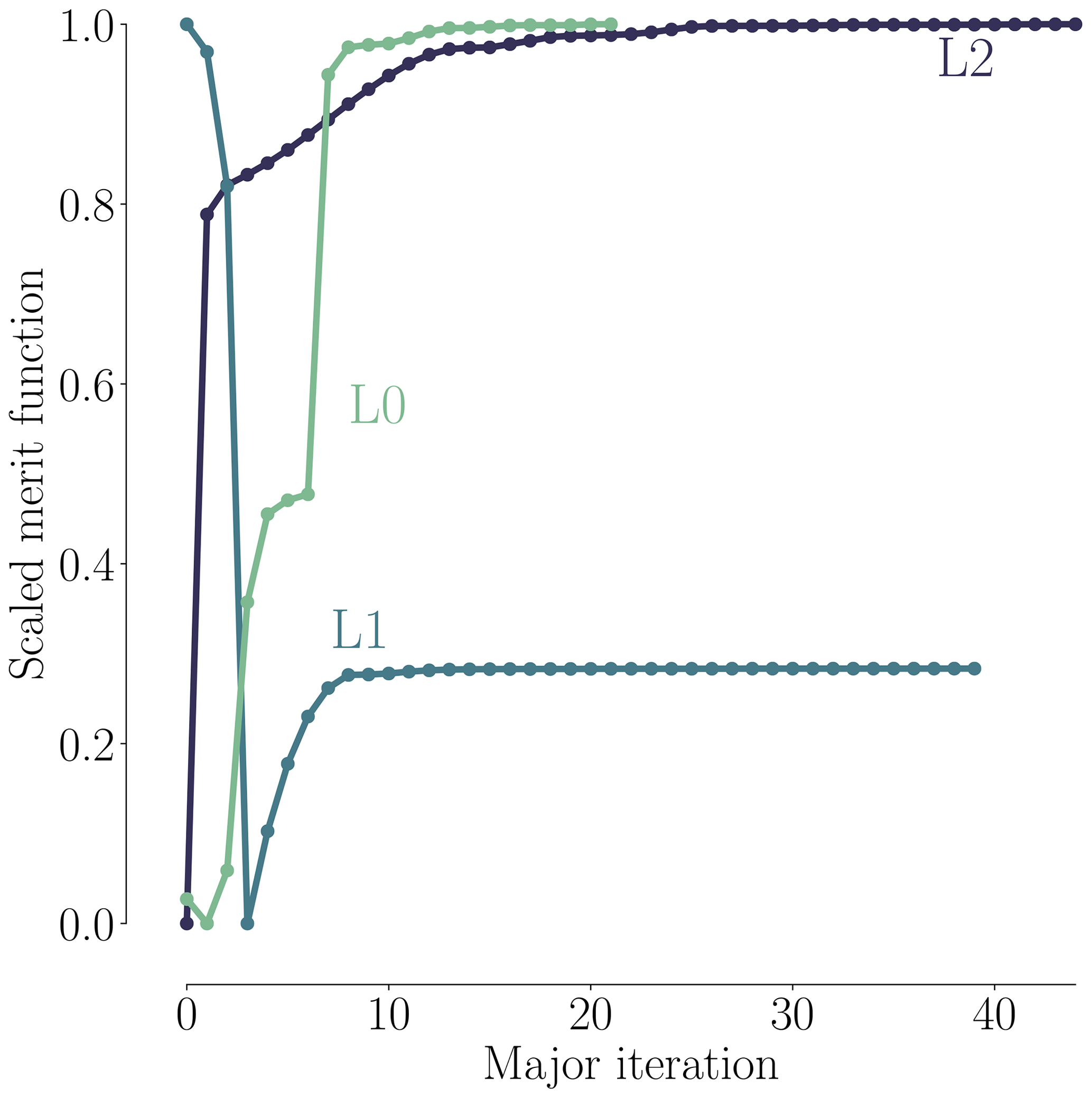
As shown in Fig. 8, all optimizations converged to an optimality of at least 10−4 (black dashed line). Figure 9 shows the merit function, which combines the scaled objective function value and constraint feasibility. The merit function value is equivalent to the scaled objective function value when all constraints are satisfied towards the end of the optimization process. As we can see in Fig. 9, the curves flatten towards the end, and further iterations are not worthwhile because the optimizer reaches the limit of what it can achieve with the provided precision of the function evaluations. The pitch optimizations are summarized in Table 6.

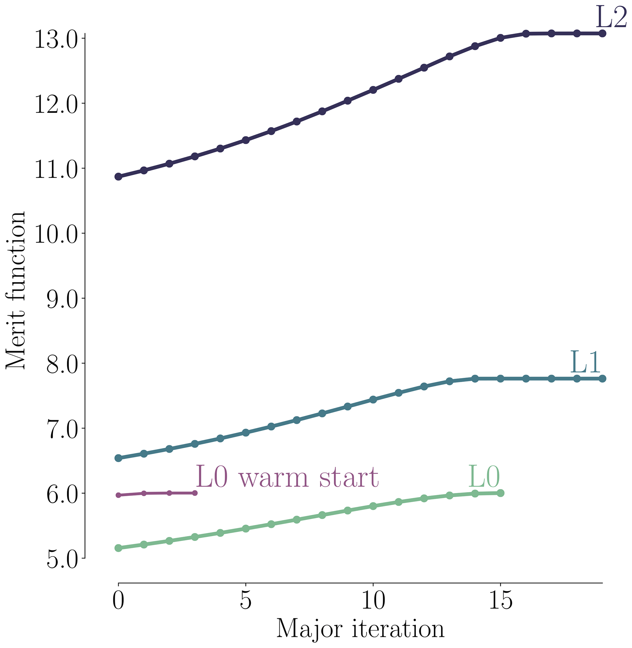
Table 6Pitch design variable optimization. All runs used 216 processors. This means that, for example, the L2 optimization had an actual wall-clock time just under 30 min.

* Warm start with the L2 optimum, resulting in a total CPU time of 106.9 h + 6436.3 h = 6543.2 h.
6.2 Planform optimization
For the planform optimization, described in Sect. 5.1, both twist and chord are controlled at the seven outer FFD sections along the blade, which results in 14 design variables. The high-fidelity planform optimization results are visualized in Figs. 10–12, which show the final chord and twist distributions as well as the history of the convergence and merit functions.
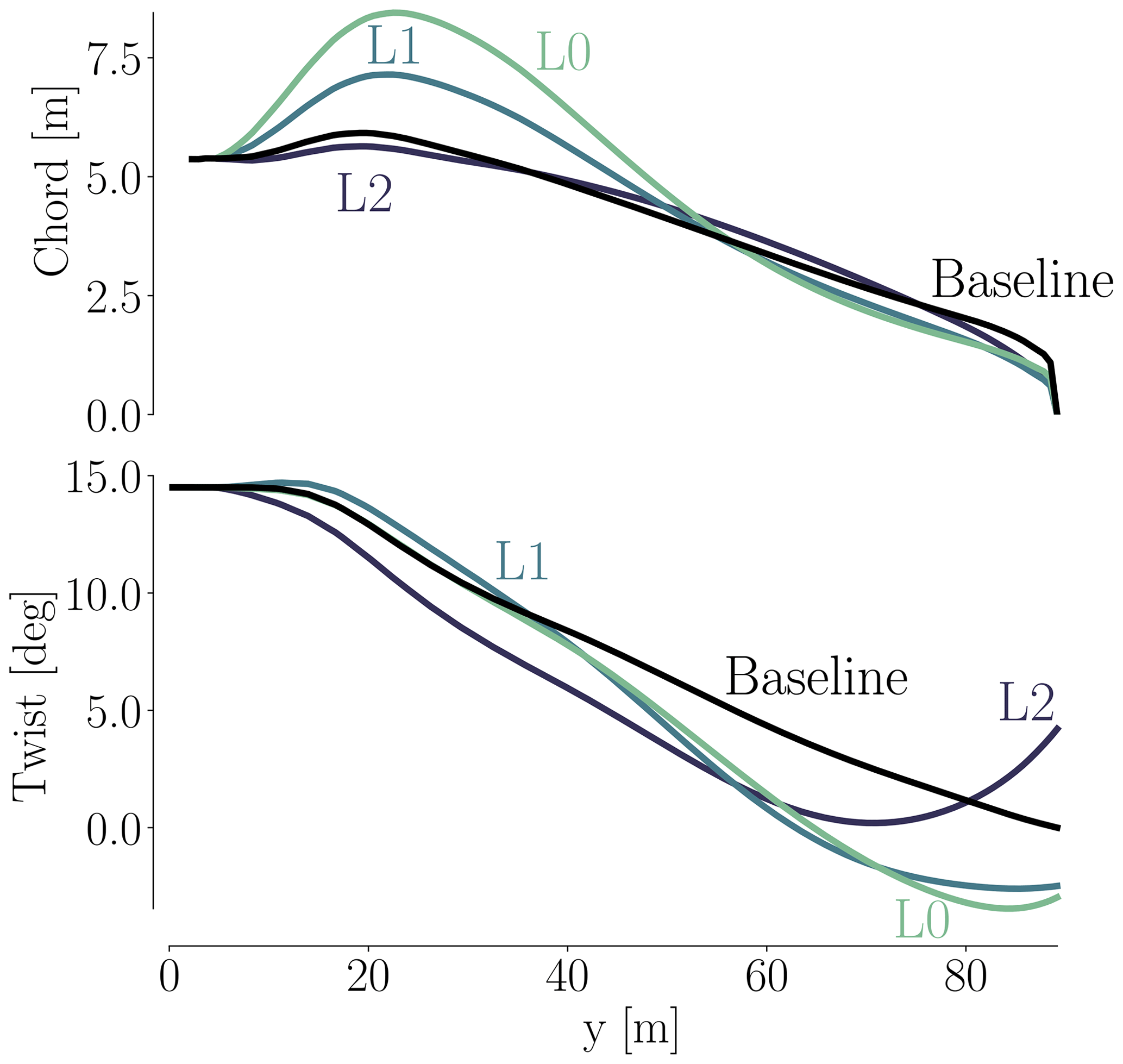
As we can see in Fig. 10, the optimized shape for the finest mesh level has a large increase in chord towards the root and a decrease in chord towards the tip, just as we would expect for an aerodynamically optimized blade. The optimized chord distribution is reminiscent of the DTU 10 MW turbine's chord distribution from Fig. 2, which was also designed for maximum power. However, the DTU 10 MW root chord is not as high due to a constraint on maximum chord of 6.2 m. Turning to the optimized twist (green curve) in the lower plot in Fig. 10, we see it exhibits a large variation towards the tip compared to its baseline. The result is a more aggressive twist distribution.
Comparing the results across mesh levels, there is a much larger spread than for the pitch optimization. The result using the coarsest (L2) mesh is significantly different from the ones obtained with the finer meshes (L1 and L0); therefore, the L2 mesh is too coarse to obtain physically representative results, which is consistent with the mesh convergence study (Table 4). We cannot rule out that, in some cases, the L2 result can be useful to perform a warm start sequence, as shown for the pitch optimization (Fig. 7 and Table 6). However, the planform results certainly show that one should use the L2 mesh with care and not for final results.
Figure 11 shows the convergence history for the three mesh levels. Again, all optimizations were converged to at least 10−4. In Fig. 12, we see a similar trend to that of the pitch optimization (Fig. 9), where much of the improvement is gained in the first half of the optimization. Thus, an easy way to speed up the design process would be to take an intermediate design. However, one should make sure to check the constraint feasibility, since SQP methods often explore infeasible regions before fully converging. The sharp initial decrease for L1 is due to the (infeasible) warm start from L2. Note that the function is scaled differently for each mesh level to accommodate all the results in one figure.
We now compare our L0 result from the planform optimization to our results from the BEM1 and BEM2 optimization problems. We obtain the BEM results by running HAWTOpt2 (Zahle et al., 2016), which uses HAWCStab2 (Hansen, 2004) as the underlying analysis code. Since this is a comparison between results obtained with completely different models, we do not expect an exact match, but we expect similar trends. As previously mentioned, the CFD planform optimization problem and the BEM1 optimization are completely identical in problem definition, and the relative thickness is fixed in both optimizations. For the BEM2 optimization, the main difference is that it is solved as a multipoint optimization and that the relative thicknesses can be changed through interpolation. We refer to Sect. 5 for further information.
The BEM optimizations are performed with SNOPT. The baseline and optimized chord and twist distributions are shown in Fig. 13. Although both chord and twist distributions show clear discrepancies for the final designs, there are several similar traits. When it comes to chord, there is a large difference in maximum chord. BEM1 converges to a 26 % increase, BEM2 converges to a 74 % increase, and the CFD optimization converges to somewhere between these two (43 %). BEM1 is the surprising result of the three, because it seems that the relation between power and thrust is so poor that it makes little sense to increase the chord at the root. This is owed to the fact that BEM1 has fixed relative thickness for all sections. It makes sense that BEM2 can increase the chord further since it can change the relative thickness. Given that our CFD-based planform optimization also has fixed relative thickness, it also makes sense that the BEM2 chord values are larger than those from the CFD-based planform optimization.
Both the BEM1 and the BEM2 results have a steeper, more pronounced increase in chord values, which we suspect our CFD framework could not reproduce due to difference in the parameterization. The two innermost fixed FFD sections ensuring the C1 mesh continuity make such a steep increase in chord impossible so close to the root. As a final comment on the discrepancies at the root, we suspect that BEM profile data for such thick airfoils are far from precise. Besides, the empirical 3-D correction used on said 2-D profile data is also likely to be imprecise. Needless to say, the combination of the two could yield shaky results. To make matters worse, we know from the comparative analysis (Fig. A3) that separation reaches up to about 37 m span, which further complicates the situation. A more uniform picture is seen for the tip region where the chord distributions have converged to a reduced chord, where only minor differences can be seen. In conclusion, the overall trends in optimal chord distribution are mirrored across the BEM and CFD models, and the discrepancies are less pronounced towards the tip.
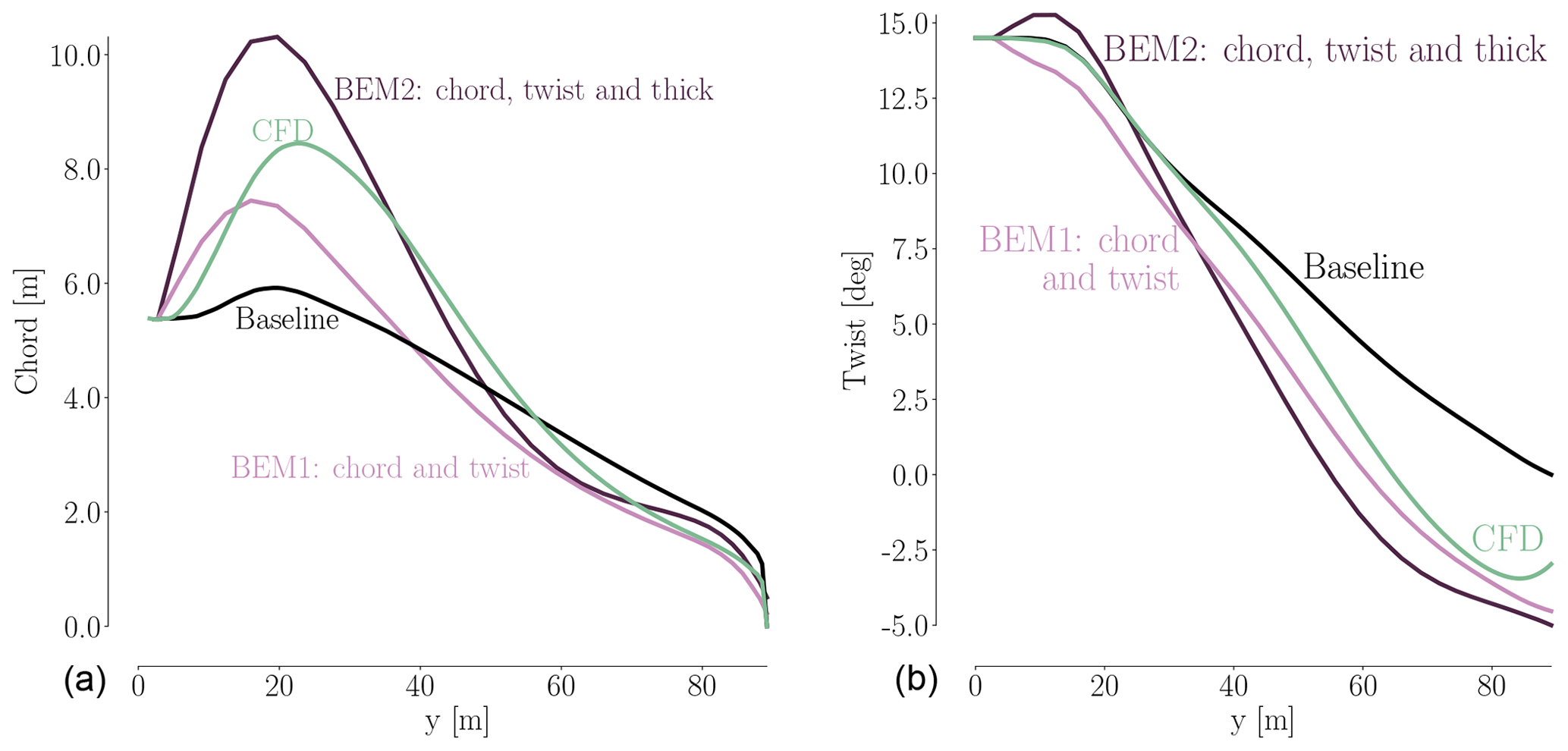
Figure 13Comparison between optimal chord (a) and twist (b) distributions for the IEA Wind Task 37 case study. The three design optimization problems – (i) single-point planform optimization, (ii) BEM1, and (iii) BEM2 – are further described in Sect. 5.1.
As for the twist comparison (Fig. 13b), both CFD and BEM results exhibit the overall trend of decreasing the twist relative to the baseline, but the BEM twist is consistently 1–2∘ lower than the CFD result. This difference is likely due to the different modeling. The CFD parameterization is limited near the root due to the two fixed sections that enforce C1 continuity, so it cannot match the more abrupt change in twist for the BEM result in that region. The BEM2 result exhibits an increase in twist near the root, which is very different from the BEM1 trend. This is because BEM2 is free to control the chord while lowering the relative thickness. Thus, BEM2 uses a large chord increase near the root to optimize the loading, instead of using twist. The planform optimization and BEM comparison are summarized in Table 7.
Table 7Planform optimization comparison between CFD and BEM results.
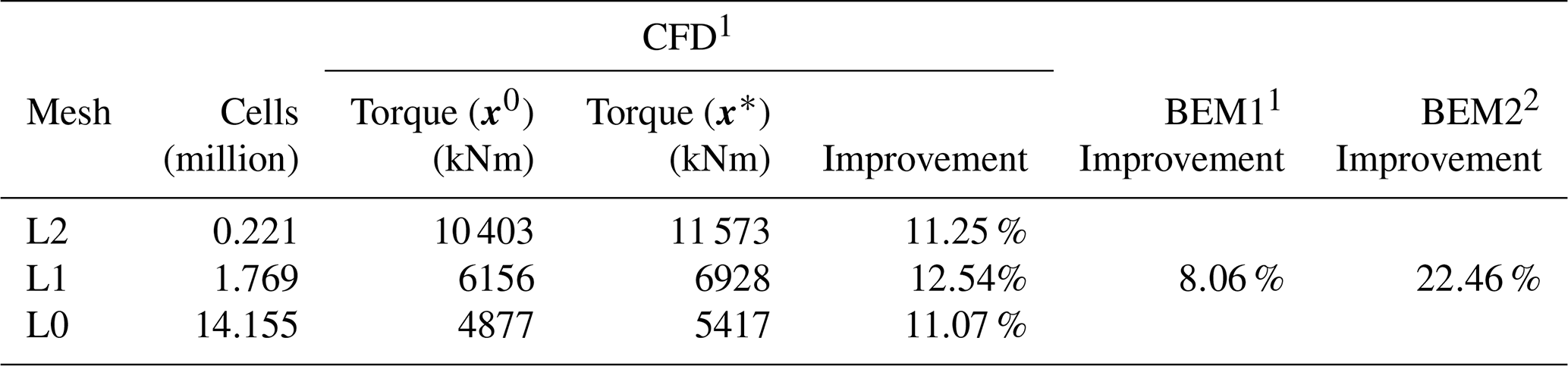
1 Relative improvement in torque. 2 Relative improvement in AEP.
Using values for torque from Table 7, we can obtain the power coefficient, CP, defined as
where P is power, ρ is the air density, V is wind speed, and A is the area swept by the rotor. The resulting coefficients are for mesh levels L2, L1, and L0, respectively. Clearly, the coarser the mesh, the more unphysical the coefficient. The Betz limit for power coefficients () is violated for L2 and L1, which draws the results from coarse mesh levels into doubt. Judging from the huge spread in these coefficients, it is not surprising that the optimized designs differ greatly across mesh levels.
6.3 Single-point shape optimization
We now solve the full shape optimization problem as a single-point optimization. As stated in Sect. 5, this problem is equivalent to optimizing for torque, when only a single wind speed is used. Figure 14 shows convergence (left) and scaled merit function (right) histories for the free-form shape optimizations. Since we typically request an optimization convergence tolerance that is smaller than what is possible for the level of the CFD solver convergence, the optimizer stops before the optimization convergence tolerance is met. Comparing the convergence history to similar plots for the pitch and planform optimizations (Figs. 8 and 11), we see that as the mesh is refined, the optimization is better converged, and the finest mesh level almost meets the requested tolerance (black dashed line). However, the scaled merit function plots (Fig. 14b) do seem flat for L2 and L1 (albeit the latter curve is less smooth), hinting that the merit function could have plateaued.
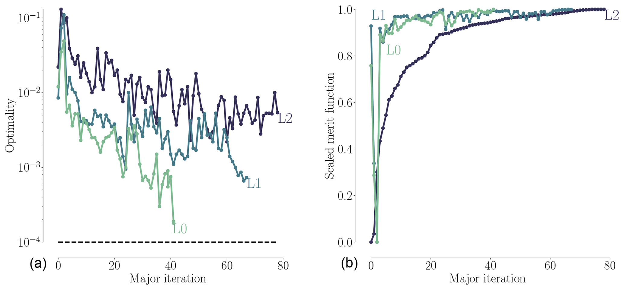
Figure 14Convergence history (a) and scaled merit function history (b) for the single-point shape optimizations.
Table 8 shows the improvement achieved by the optimization. The achieved improvement on the finest mesh (15.89 %) is higher than that of the planform optimization (11.07 %, Table 7), which is expected because this case includes all the planform design optimization variables plus the additional freedom to optimize the airfoil shapes. One should not compare these results to the pitch optimization results since they do not include any thrust constraint. A comparison to the BEM code results is given farther down in Table 9 once the multipoint optimization results have been presented.
Table 8Overview of single-point optimization results for the operational conditions of the 8 m s−1 case listed in Table A1.

We now turn to the shape and pressure (Cp) distributions for the baseline and optimized geometries in Fig. 15. The optimized blade increases the chord near the root. This design trend agrees with the planform optimization result.

Figure 15Comparison of Cp distributions for the baseline and optimized result from the single-point shape optimization. There is an increase in TE camber, especially at the root, as well as a less pronounced suction peak.
Comparing the airfoil shapes and corresponding Cp distributions at the bottom of Fig. 15, we can see that the optimization reduced the thickness and slightly increased the camber. The thickness reduction is expected when considering only the aerodynamics with no structural strength constraints. Since we use thickness constraints as a surrogate for structural feasibility, the optimizer exploits this by producing the thinnest airfoils that satisfy these constraints. The increased camber, owed to the physical incentive to generate more lift, is consistent with the results of Dhert et al. (2017), but the increase in camber here is more modest because the optimizer can increase the torque by tailoring camber, chord, and twist instead of just camber. The incentive to operate at high lift coefficient is due to the fact that high Cl∕Cd is most easily achieved by operating at high Cl, especially for airfoils designed assuming a fully turbulent boundary layer.
Another feature of the optimized airfoil shapes is the sharper LE. This is expected due to the fact that we are maximizing the performance at a single wind speed. This shape is not robust to changes in wind speed and would perform poorly at other wind speeds. This issue can be addressed by enforcing the LE radius constraints or by considering the performance for multiple wind speeds in the objective function, as we will see in the next section.
6.4 Multipoint shape optimization
The motivation for this multipoint optimization is to take a whole range of wind speeds into consideration to achieve a more robust design. We consider both cases for normal power production and also cases leading to peak loading conditions. The design optimization problem and model are the same as those for the single-point optimizations (detailed in Sect. 5.1), except for the objective function. The objective function here is the AEP estimate, which we describe in Sect. 5.1.
When it comes to selecting the wind speeds in a multipoint optimization, it is important to consider speeds that lie outside the ideal operational range. Typically, the rotational rate of the wind turbine rotor is controlled to match a target tip speed ratio, which is the ratio of the tip speed and the wind speed, given by . As long as the tip speed ratio is the same, the blade angle of attack is the same, and a given design has similar aerodynamic performance. However, for low wind speeds, the rotational speed has a lower bound to avoid tower excitation, and at higher wind speeds, the rotational speed is kept constant, and the turbine starts regulating pitch to maintain rated mechanical power. In our case, the target tip speed ratio is λ=7.8, and the rotor speeds corresponding to the minimum and maximum limits are 6.0 and 9.6 rpm, respectively. The variation of rotor speed with wind speed is shown in Fig. 16. There are two reasons we consider wind speeds outside the constant tip speed ratio range. First, the angles of attack are different at these operating points, which should lead to a more balanced design. Additionally, we need to consider the load constraints defined in the optimization case study. For this reason, we choose 5 m s−1 as the lower wind speed, and 11 m s−1, because this is just below the wind speed at which the rotor reaches rated rotational speed and rated power and thus peak thrust and flapwise moment.
Research has shown that, in reality, the angle of attack varies significantly (more than 4∘) over just one rotor revolution (Madsen et al., 2014, Fig. 5). The explanation for this can be found in the complex operating conditions for turbines containing, for example, turbulent inflow and inflow wind shear. To simulate these effects, it would be ideal to add turbulent inflow and transition from steady-state RANS to unsteady RANS. A cheaper way could be a multipoint optimization with a fixed rpm for all turbines operating at slightly different wind speeds. We leave this for future work.
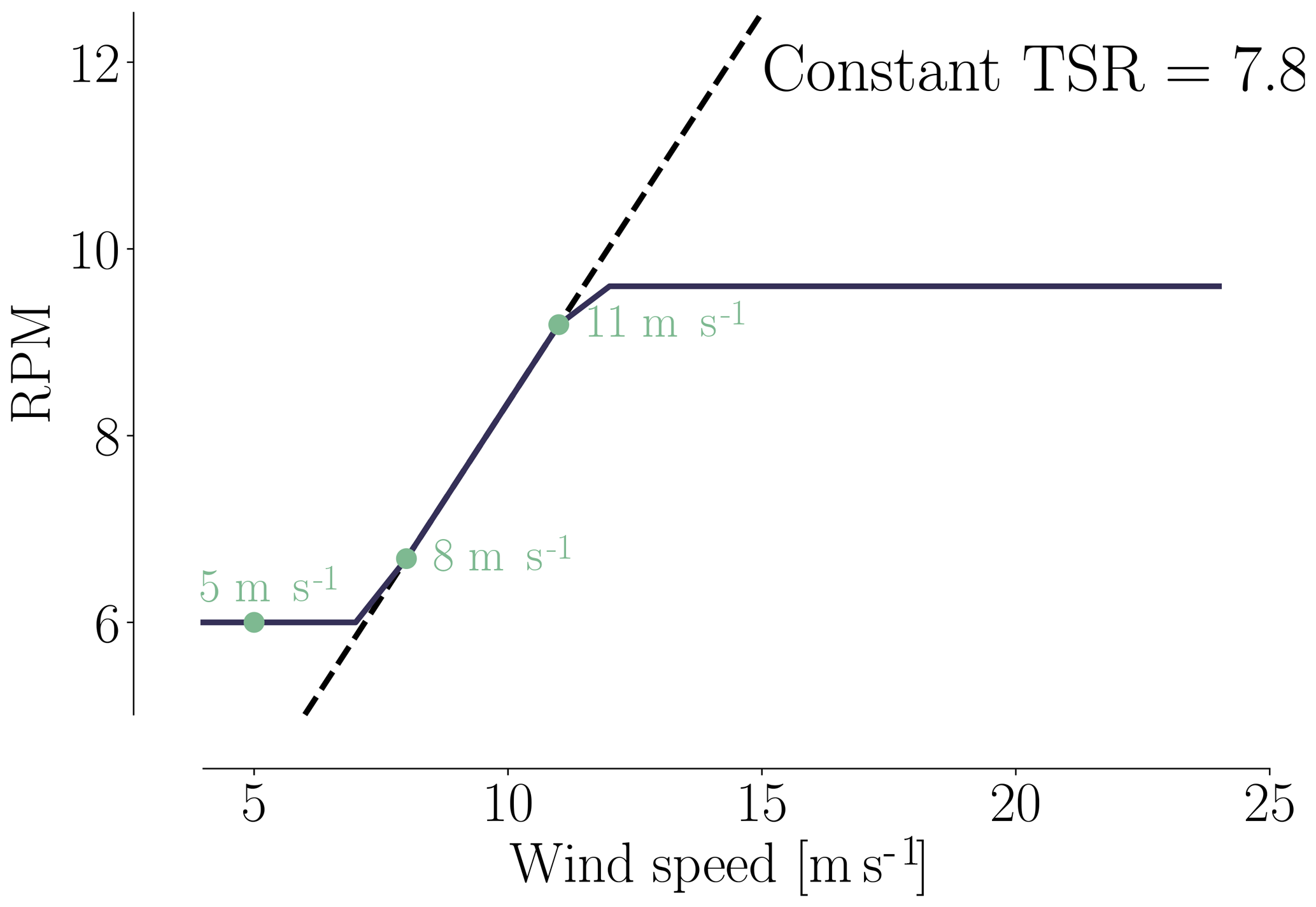
Figure 16Rotational rate schedule with wind speed, showing the ideal constant tip speed rate. The green dots are the wind speeds used in the multipoint optimizations.
The history of convergence and merit functions are shown in Fig. 17. Just as for the single-point optimization, the selected threshold is not quite met. However, as before, the scaled merit function flattens enough that we determined that the design is close enough to the optimum.

Figure 17History of convergence (a) and scaled merit functions (b) for the multipoint shape optimizations.
We first turn to the airfoil shape to assess the effect of adding geometrical constraints while taking multiple angles of attack into consideration. The airfoil shapes for the multipoint optimizations are compared to the single-point ones in Fig. 18. As we can see, the LE shapes are somewhat improved but still unrealistically sharp. This points towards the necessity of including off-design operational cases resulting in wider ranges of angles of attack, where such a sharp LE would result in deterioration in performance.

Figure 18Comparison of airfoil profiles obtained from single-point and multipoint optimizations. The profiles are taken from 35, 64, and 84 m spanwise positions.
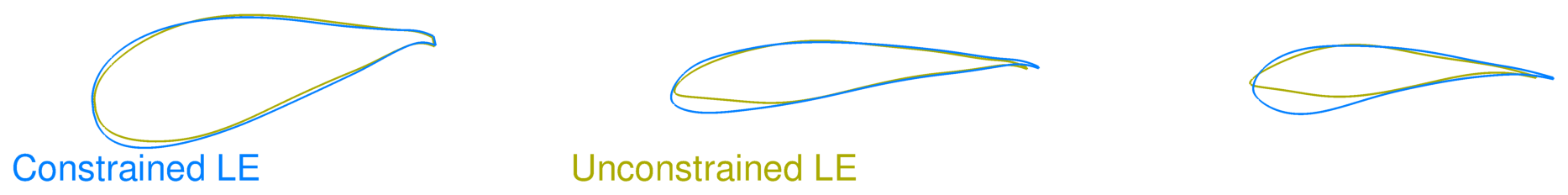
Figure 19Comparison of airfoil profiles obtained from multipoint optimizations with and without LE geometric constraint.
To obtain more realistic LE shapes, we added an LE thickness constraint to the optimization problem. The geometric constraint was enforced as a thickness constraint close to the LE. The resulting shapes are shown in Fig. 19, where we compare them to the shape obtained by the multipoint optimization without the LE constraints. While we choose to focus solely on the 2-D profile improvement from single-point to multipoint optimizations, the optimizations are indeed all 3-D rotor optimizations. As we can see, enforcing the geometric constraint results in a more round LE shape that is much more similar to previously published wind turbine airfoil shapes.
Having verified that the resulting shapes for the multipoint full shape optimizations are much improved, we now compare the multipoint optimization results to other optimization results in Table 9. Whereas the single-point BEM1 result (8.06 %) is close to the single-point planform optimization result (11.07 %), the multipoint BEM2 result (22.46 %) is comparable to the multipoint full shape optimizations result (23.76 %) since relative thicknesses can change in both cases. The multipoint result (23.76 %) is somewhat higher than the single-point full shape optimization result (15.89 %), which can be explained by the relaxed thrust constraint for multipoint optimizations. Here, we use the thrust from the 12 m s−1 case instead of the 8 m s−1 case to define the initial constraint values for thrust and bending moment. Indeed, the thrust constraint relaxation results in the constraint not being active at convergence for the CFD-based multipoint full shape optimization, as seen in Table 9.
These results do not show that the industry can necessarily gain a 20 % increase simply by using high-fidelity optimization. Indeed, the amount of improvement depends on the performance of the baseline turbine. Since we study an intentionally poor baseline design, we therefore get a large improvement.
Table 9Overview of optimization results. As further detailed in Sect. 5.1, the single-point and multipoint optimizations use the operational conditions for the 8 m s−1 case and 5, 8, and 11 m s−1 cases, respectively. Operational conditions are listed in Table A1.
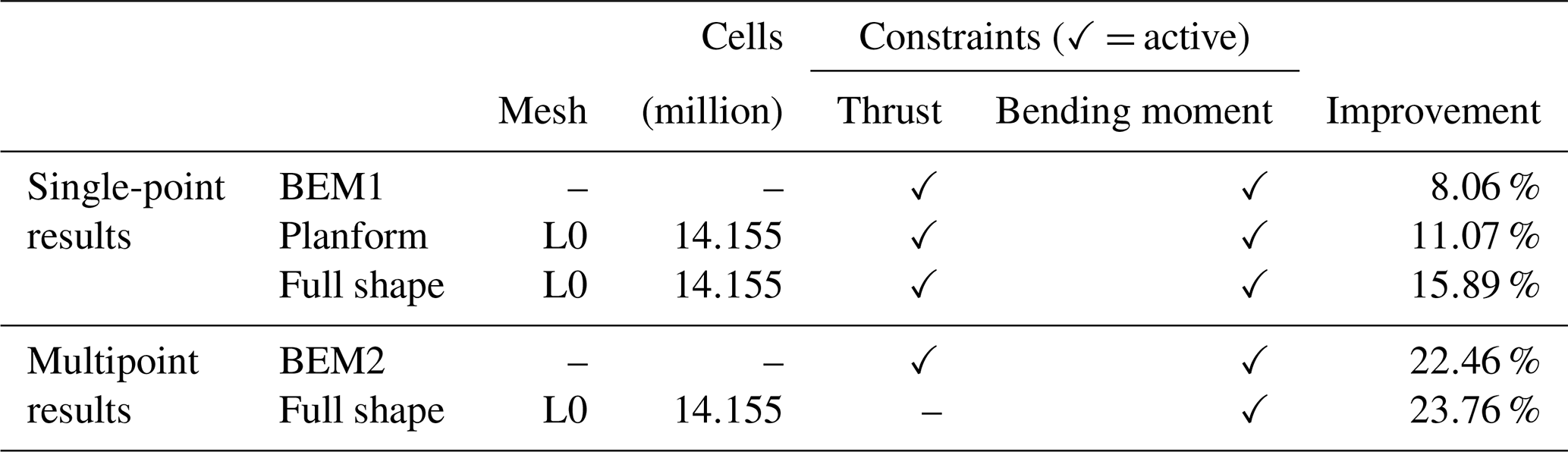
To analyze the optimized designs from single-point and multipoint shape optimizations in more detail, we plot the spanwise forces for both optimized and baseline designs in Fig. 20.
The normal force acts normal to the rotor plane and, integrated over all three blades, yields the rotor thrust. Likewise, the torque can be derived from the driving force by integrating its first moment along all three blades.
For the single-point shape optimization results, we see, as expected, an overall large increase in tangential loading across the blade, and we observe that a high loading is achieved in the root region of the blade as well. This is partially due to the chord increase but also due to the fact that the blade is optimized based on modeling that accounts for the complex three-dimensional flow field, which is particularly dominant in the root region. The thrust constraint and moment constraint were both essential for the design to be industrially relevant for the single-point result: the thrust constraint helped lower the overall thrust values to maintain structural feasibility. The bending moment constraint resulted in a change in the normal force distribution, where the peak moved farther inboard to reduce high loads close to the tip region, as one would expect. Based on the optimization output, we can verify that both constraints are active for the single-point optimization, meaning that thrust and moment have reached the upper limits of 14 % and 11 % increase in thrust and moment, respectively. In the multipoint full shape optimization, the moment constraint is again active at an 11 % increase in bending moment. However, the thrust constraint is only at 11 % and is, as mentioned, not active at convergence due to the relaxed constraint. With these constraints, we could add span as a design variable in future work.
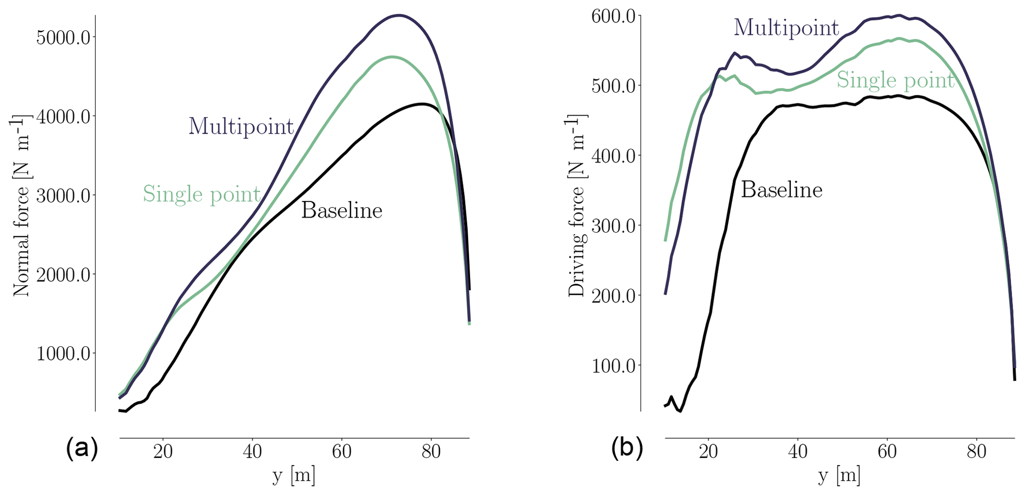
Figure 20Comparison of normal (a) and driving (b) forces for baseline and optimized designs. The shape optimization increases the normal force, and the peak has also moved further inboard. The driving force is increased considerably both at the root and close to the tip region.
We find the same overall trends for the multipoint results as we did for the single-point optimization. The relaxed thrust constraint for the multipoint optimization results in a rotor with slightly higher loads, which explains why the more robust design from the multipoint optimization outperforms the single-point result.
The multipoint optimization problem presented in this section is functional but should be further improved in the future to obtain truly practical wind turbines. First, the laminar to turbulent boundary layer transition should be modeled, since this affects the optimal airfoil shapes. In this work, we just assumed the boundary layer to be turbulent throughout. Second, a wider range of operating points should be considered by, for example, varying the rotation rate or pitch setting for a given wind speed.
In this work, we presented results from the high-fidelity RANS-based shape optimization of a 10 MW RWT. Based on our literature review of the high-fidelity shape optimization efforts in wind turbine design, we determined that this was a promising area of research.
We compared two state-of-the-art compressible and incompressible CFD solvers to quantify the mesh dependence and discrepancies across different RANS models applied on the same rotor. The results were compatible, and future work involving classical compressibility corrections was identified.
We investigated the advantage of using higher-fidelity models by comparing our optimization results to low-fidelity BEM results from the same case study. We did this through a planform optimization with chord and twist variables, where shape changes were restricted to keep the design case comparable with the BEM-based optimization. The overall design trends were the same across fidelities, with differences due the parameterizations and models. The same overall amount of improvement was observed.
Finally, full shape optimization was performed with respect to twist, chord, and airfoil shape design variables, which raised the number of design variables from 14 to 154. Here, the planform results were further improved with a factor of 1.44. The improvement was enabled by a decrease in relative thickness as well as the novel airfoil shapes.
While further developments are required to obtain truly practical wind turbine blade shapes, this work shows that with the right tools, we can model the entire geometry, including the root, and optimize modern wind turbine rotors at the cost of 𝒪(102) CFD evaluations.
Data are available upon request to the corresponding author.
The following is a continuation of Sect. 4 to extend the comparison between the flow solvers: EllipSys3D and ADflow.
Table A1Operational conditions for the simulations in the analysis. For the compressible solver (ADflow), we use velocity, density, and temperature as input parameters. ADflow then computes the complete thermodynamic conditions. The density is set to 1.225 kg m−3, temperature to 15 ∘C, and dynamic viscosity to kg m−1 s−1.
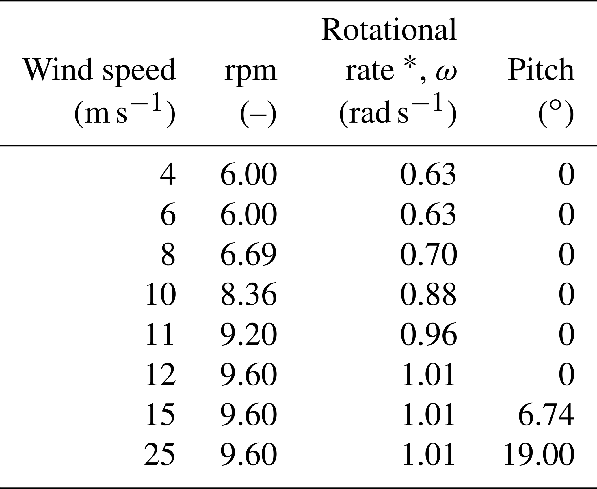
* Based on a target tip speed ratio of γ=7.8, where .
A1 Operational conditions
The case study is defined with a cut-in speed of 4 m s−1 and a cut-out speed of 25 m s−1. Within this range, we use the eight operational conditions defined in Table A1 to compare the solvers.
A2 Integrated loads
Integrated loads, in the form of thrust and torque, have been computed for each simulation in Table A1 and are visualized in Fig. A1. As seen, the ADflow results are consistently higher than the EllipSys3D results. This trend could partially be accounted for by applying the mentioned Prandtl–Glauert correction to the incompressible computations but is also a result of ADflow results on mesh L0 not being fully mesh independent, as shown in Table 4. As a low-fidelity reference, we have added the integrated loads (in gray) from steady-state BEM results using HAWCStab2. A general agreement between the CFD results and the HAWCStab2 results can be seen, save for the torque value at 25 m s−1, which could be corrected with a slight change in pitch setting given in Table A1. Agreement is expected between EllipSys3D and BEM since the airfoil data used in BEM are computed using EllipSys2D.
A3 Spanwise forces, pressure distribution and flow visualization
Figure A2 shows the spanwise forces and shows that the difference between solvers is more or less spread out over the entire span. Not surprisingly, the ADflow values are consistently higher. We will revisit the distribution of spanwise forces after the optimization to inspect where performance increase occurs on the blade.
Turning to the surface-restricted streamlines in Fig. A3, we first note the rather large amount of separation. Even the pressure side shows a distinct area of separation from 19 to 41 m span. Comparing said area with the pressure side separation for the unperturbed DTU 10 MW rotor in Fig. A4, where only a small separation area at the root is seen, it is clear that the perturbed design we use as a starting point for the optimization seen in Fig. A3 suffers a more poor aerodynamic design owed to the reduced chord distribution and increase in relative thickness. The suction side in Fig. A3 looks more like one would expect, save for the expanded separation area reaching just above 37 m in the spanwise direction. Here, the DTU 10 MW only has separation below the 32 m span, as seen in Fig. A4.
In Fig. A5, we compare the obtained Cp curves at three spanwise positions: 35, 64, and 84 m (positions marked in red in Fig. A3), where the Cp distribution is found using the dynamic pressure, and the far-field pressure, p∞:
The slice at 35 m shows the least consistent comparison, which we suspect is due to the large amount of separation present both at suction and pressure side. Given that the solvers use different turbulence models, it would be surprising to find a perfect match at this position. We also note that the pressure side separation results in a Cp curve with a typical flat, squeezed shape in the 30 % closest to the trailing edge (TE). The Cp curves for the sections at 64 m span and 84 m span show, in general, a better likeness to one another. Early investigations showed that the chordwise distribution of cells has a distinct impact on the solvers' ability to capture the stagnation point and suction peak. Therefore, we chose a distribution that seemed to have enough cells close to the stagnation point while still having an adequate amount of cells to resolve the TE area. In general, the ADflow suction peaks seem to be more pronounced than those from EllipSys3D. The same can be said for the blunt TE, where the ADflow Cp curve again has a more pronounced spike.
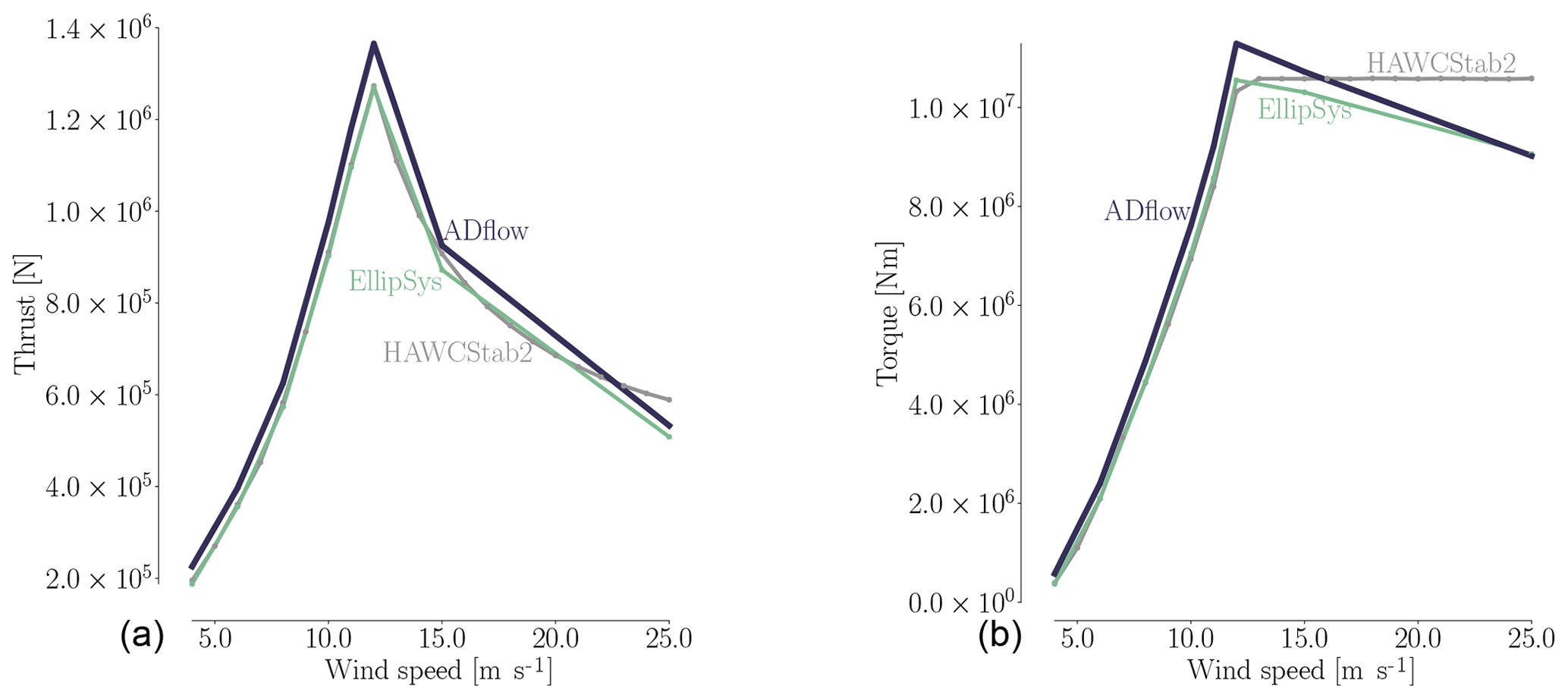
Figure A1Total thrust (a) and torque (b) as a function of wind speed for the rotor geometry used as the starting point for the optimization computed using mesh L0. As expected, the torque increases rapidly from cut-in speed to the rated speed at 12 m s−1, which is also where the thrust peak occurs. From rated to cut out, the torque curve flattens. Here, the pitch setting found with steady-state BEM results using HAWCStab2 (seen in gray) clearly does not result in the CFD solvers tracking rated power accurately due to the model changes. ADflow consistently overshoots the EllipSys results, which is consistent with the trend seen in Table 4. Operational conditions for the eight simulations are given in Table A1.
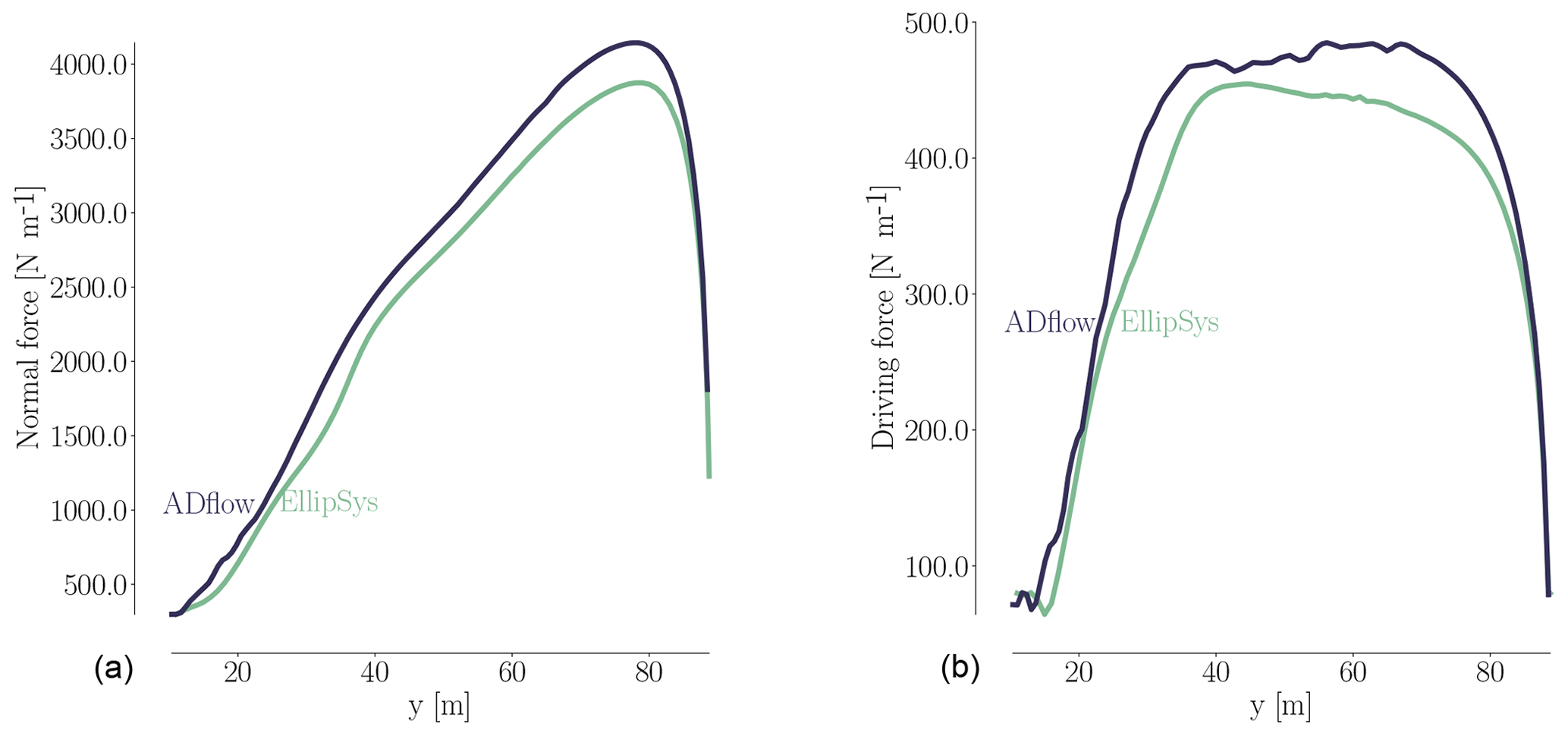
Figure A2Spanwise distribution of the normal force (a) and driving force (b) for the 8 m s−1 case listed in Table A1.
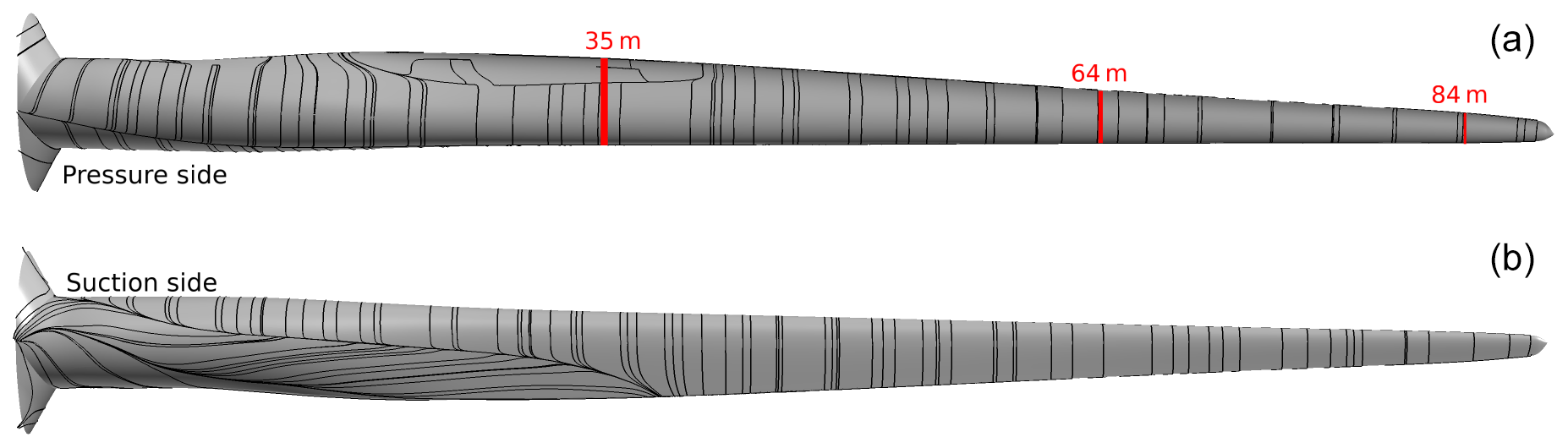
Figure A3Surface-restricted streamlines from the EllipSys solution for a wind speed of 8 m s−1, both for the pressure side (a) and the suction side (b) for the perturbed design we use as a starting point for the optimization. The operational conditions are listed in Table A1.
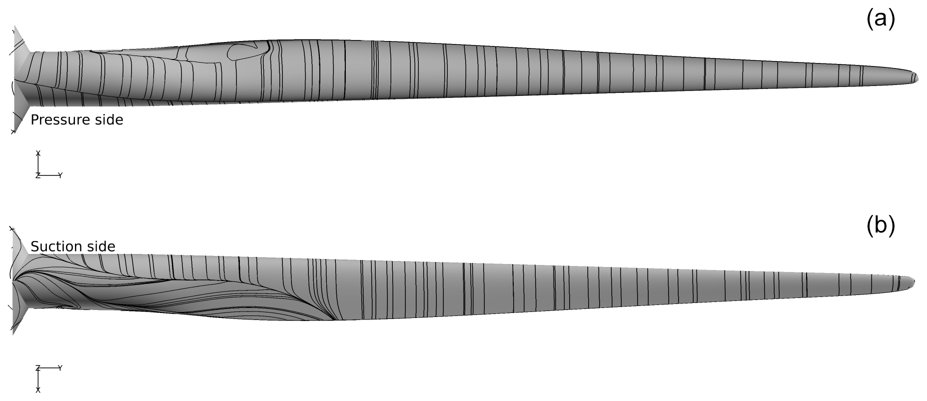
Figure A4Surface-restricted streamlines from the EllipSys solution obtained using the original DTU 10 MW wind turbine geometry for the 8 m s−1 case in Table A1 both for the pressure side (a) and the suction side (b).
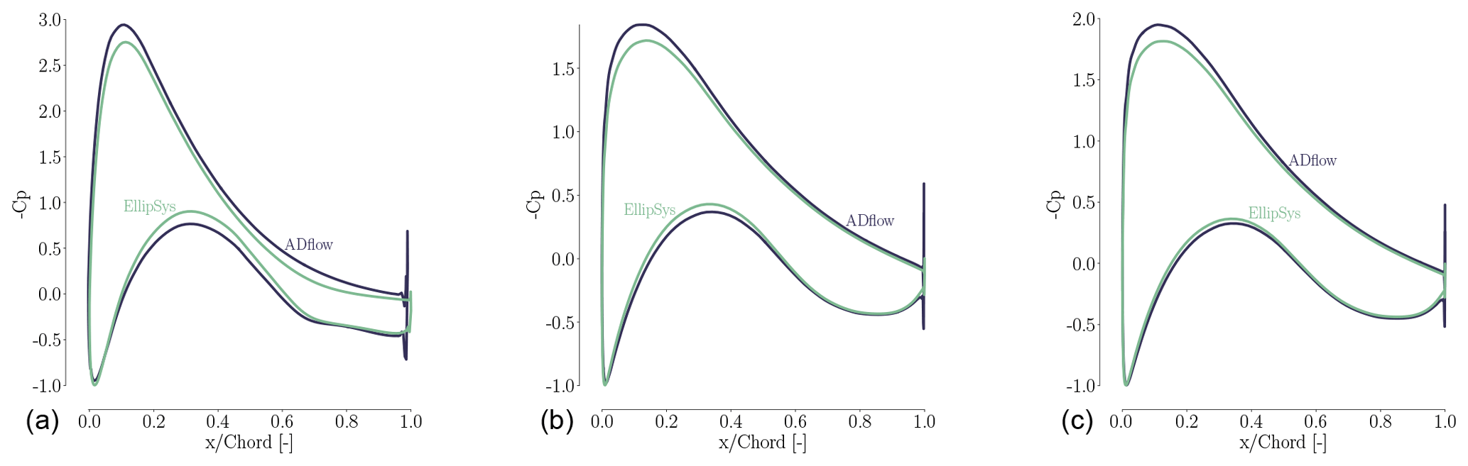
MHAM compiled the literature review, implemented the geometry constraint and the algorithmic differentiation contributions, created the FFD boxes and CFD meshes for the test cases, ran the analysis and optimizations, postprocessed the cases, and wrote the bulk of the paper. FZ assisted in work related to CFD meshes, analysis and optimization, and carried out all BEM optimizations. NNS assisted with CFD expertise within mesh generation, CFD solver settings, and issues related to compressibility effects. JRRAM guided the project, secured access to clusters, and gave technical advice on the entire tool chain at the University of Michigan. All authors took part in writing and editing the paper.
The authors declare that they have no conflict of interest.
We would like to thank the members of the MDO Lab for their support. We thank, in particular, Eirikur Jonsson for assistance with programs in the MACH framework, Nicholas Bons for helping with pyGeo, and Anil Yildirim for his assistance with the ANK solver. We also thank Charles A. Mader for consulting on the AD improvements implemented in the adjoint solver. Finally, researcher Michael McWilliam at DTU kindly assisted with IEA material.
This paper was edited by Alessandro Bianchini and reviewed by Joseph Saverin and one anonymous referee.
Anderson, E., Bhuiyan, F., Mavriplis, D., and Fertig, R.: Adjoint-Based High-Fidelity Aeroelastic Optimization of Wind Turbine Blade for Load Stress Minimization, 2018 Wind Energy Symposium, AIAA SciTech Forum (AIAA 2018-1241), https://doi.org/10.2514/6.2018-1241, 2018. a
Ashuri, T.: Beyond Classical Upscaling: Integrated Aeroservoelastic Design and Optimization of Large Offshore Wind Turbines, PhD thesis, Delft University of Technology, Delft, the Netherlands, 2012. a
Ashuri, T., Zaaijer, M. B., Martins, J. R. R. A., van Bussel, G. J. W., and van Kuik, G. A. M.: Multidisciplinary Design Optimization of Offshore Wind Turbines for Minimum Levelized Cost of Energy, Renew. Energ., 68, 893–905, https://doi.org/10.1016/j.renene.2014.02.045, 2014. a
Ashuri, T., Martins, J. R. R. A., Zaaijer, M. B., van Kuik, G. A., and van Bussel, G. J.: Aeroservoelastic Design Definition of a 20 MW Common Research Wind Turbine Model, Wind Energy, 19, 2071—2087, https://doi.org/10.1002/we.1970, 2016. a
Badreddinne, K., Ali, H., and David, A.: Optimum project for horizontal axis wind turbines “OPHWT”, Renew. Energ., 30, 2019–2043, https://doi.org/10.1016/j.renene.2004.12.004, 2005. a
Bak, C., Zahle, F., Bitsche, R., Kim, T., Yde, A., Henriksen, L., Natarajan, A., and Hansen, M.: Description of the DTU 10 MW Reference Wind Turbine, Tech. rep., Risø National Laboratory, 2013. a, b
Balay, S., Gropp, W., McInnes, L., and Smith, B.: Efficient management of parallelism in object oriented numerical software libraries, in: Modern Software Tools in Scientific Computing, edited by: Arge, E., Bruaset, A. M., and Langtangen, H. P., Birkhäuser Press, 163–202, 1997. a
Balay, S., Abhyankar, S., Adams, M., Brown, J., Brune, P., Buschelman, K., Dalcin, L., Eijkhout, V., Gropp, W., Kaushik, D., Knepley, M., May, D., McInnes, L., Mills, R., Munson, T., Rupp, K., Sanan, P., Smith, B., Zampini, S., Zhang, H., and Zhang, H.: PETSc Web page, available at: http://www.mcs.anl.gov/petsc (last access: 1 March 2019), 2018a. a
Balay, S., Abhyankar, S., Adams, M., JBrown, Brune, P., Buschelman, K., Dalcin, L., Eijkhout, V., Gropp, W., Kaushik, D., Knepley, M., May, D., McInnes, L., Mills, R., Munson, T., Rupp, K., PSanan, Smith, B., Zampini, S., Zhang, H., and Zhang, H.: PETSc Users Manual, Tech. Rep. ANL-95/11 - Revision 3.9, Argonne National Laboratory, available at: https://www.mcs.anl.gov/petsc/documentation/index.html (last access: 1 March 2019), 2018b. a
Barrett, R. and Ning, A.: Comparison of airfoil precomputational analysis methods for optimization of wind turbine blades, IEEE T. Sustain. Energ., 7, 1081–1088, https://doi.org/10.1109/TSTE.2016.2522381, 2016. a, b, c, d
Barrett, R. and Ning, A.: Integrated free-form method for aerostructural optimization of wind turbine blades, Wind Energy, 21, 663–675, https://doi.org/10.1002/we.2186, 2018. a, b, c, d, e, f, g
Bechmann, A., Sørensen, N., and Zahle, F.: CFD simulations of the MEXICO rotor, Wind Energy, 14, 677–689, https://doi.org/10.1002/we.450, 2011. a
Boorsma, K., Schepers, J., Gomez-Iradi, S., Herraez, I., Lutz, T., Weihing, P., Oggiano, L., Pirrung, G., Madsen, H., Shen, W., Rahimi, H., and Schaffarczyk, P.: Final Report of IEA Wind Task 29 Mexnext (Phase 3), Tech. Rep. ECN-E–18-003, https://www.ecn.nl/publications/ECN-E–18-003, 2018. a
Bottasso, C., Campagnolo, F., Croce, A., and Tibaldi, C.: Optimization-based study of bend-twist coupled rotor blades for passive and integrated passive/active load alleviation, Wind Energy, 16, 1149–1166, https://doi.org/10.1002/we.1543, 2013. a, b
Brooks, T. R., Kenway, G. K. W., and Martins, J. R. R. A.: Benchmark Aerostructural Models for the Study of Transonic Aircraft Wings, AIAA J., 56, 2840–2855, https://doi.org/10.2514/1.J056603, 2018. a, b, c
Burdette, D. and Martins, J. R. R. A.: Design of a Transonic Wing with an Adaptive Morphing Trailing Edge via Aerostructural Optimization, Aerosp. Sci. Technol., 81, 192–203, https://doi.org/10.1016/j.ast.2018.08.004, 2018. a
Burdette, D. A. and Martins, J. R. R. A.: Impact of Morphing Trailing Edge on Mission Performance for the Common Research Model, J. Aircraft, 56, 369–384, https://doi.org/10.2514/1.C034967, 2019. a
Cavar, D., Réthoré, P.-E., Bechmann, A., Sørensen, N. N., Martinez, B., Zahle, F., Berg, J., and Kelly, M. C.: Comparison of OpenFOAM and EllipSys3D for neutral atmospheric flow over complex terrain, Wind Energ. Sci., 1, 55-70, https://doi.org/10.5194/wes-1-55-2016, 2016. a
Chattot, J.: Optimization of wind turbines using helicoidal vortex model, J. Sol. Energ.-T. ASME, 125, 418–424, https://doi.org/10.1115/1.1621675, 2003. a
Chen, S., Lyu, Z., Kenway, G. K. W., and Martins, J. R. R. A.: Aerodynamic Shape Optimization of the Common Research Model Wing-Body-Tail Configuration, J. Aircraft, 53, 276–293, https://doi.org/10.2514/1.C033328, 2016. a, b
Dhert, T., Ashuri, T., and Martins, J. R. R. A.: Aerodynamic Shape Optimization of Wind Turbine Blades Using a Reynolds-Averaged Navier–Stokes Model and an Adjoint Method, Wind Energy, 20, 909–926, https://doi.org/10.1002/we.2070, 2017. a, b, c, d, e, f, g, h, i, j, k, l, m, n
Drela, M.: XFOIL: An Analysis and Design System for Low Reynolds Number Airfoils, in: Low Reynolds Number Aerodynamics, edited by: Mueller, T. J., Springer Berlin Heidelberg, Berlin, Heidelberg, 1–12, 1989. a
Drela, M. and Giles, M.: Viscous-inviscid analysis of transonic and low Reynolds number airfoils, AIAA Paper, 131–140, 1986. a
Economon, T., Palacios, F., and Alonso, J.: A viscous continuous adjoint approach for the design of rotating engineering applications, 21st AIAA Computational Fluid Dynamics Conference, San Diego, CA, 24–27 June 2013. a, b, c, d, e, f
Edward, L., Eric, C., and Eric, B.: A fast mesh deformation method using explicit interpolation, J. Comput. Phys., 231, 586–601, https://doi.org/10.1016/j.jcp.2011.09.021, 2012. a
Elfarra, M., Sezer-Uzol, N., and Akmandor, I.: NREL VI rotor blade: numerical investigation and winglet design and optimization using CFD, Wind Energy, 17, 605–626, https://doi.org/10.1002/we.1593, 2014. a, b, c
Fuglsang, P. and Madsen, H.: Optimization method for wind turbine rotors, J. Wind Eng. Ind. Aerod., 80, 191–206, https://doi.org/10.1016/S0167-6105(98)00191-3, 1999. a, b
Fuglsang, P. and Thomsen, K.: Site specific design optimization of wind turbines, A Collection of the 1998 Asme Wind Energy Symposium Technical Papers, 294–303, 1998. a
Fuglsang, P. and Thomsen, K.: Site-specific design optimization of 1.5-2.0 MW wind turbines, J. Sol. Energ.-T ASME, 123, 296–303, https://doi.org/10.1115/1.1404433, 2001. a
Fuglsang, P., Bak, C., Schepers, J., Bulder, B., Cockerill, T., Claiden, P., Olesen, A., and Rossen, R.: Site-specific design optimization of wind turbines, Wind Energy, 5, 261–279, https://doi.org/10.1002/we.61, 2002. a
Fuglsang, P., Bak, C., Gaunaa, M., and Antoniou, I.: Design and verification of the Risø-B1 airfoil family for wind turbines, J. Sol. Energ.-T ASME, 126, 1002–1010, https://doi.org/10.1115/1.1766024, 2004. a
Garg, N., Kenway, G. K. W., Martins, J. R. R. A., and Young, Y. L.: High-fidelity Multipoint Hydrostructural Optimization of a 3-D Hydrofoil, J. Fluid Struct., 71, 15–39, https://doi.org/10.1016/j.jfluidstructs.2017.02.001, 2017. a
Garg, N., Pearce, B. W., Brandner, P. A., Phillips, A. W., Martins, J. R. R. A., and Young, Y. L.: Experimental Investigation of a Hydrofoil Designed via Hydrostructural Optimization, J. Fluid Struct., 84, 243–262, https://doi.org/10.1016/j.jfluidstructs.2018.10.010, 2019. a
Garrel, A.: Development of a wind turbine aerodynamics simulation module, Tech. Rep. ECN-C–03-079, available at: https://www.ecn.nl/publications/E/2003/ECN-C–03-079 (last access: 18 March 2019), 2003. a
Gill, P. E., Murray, W., and Saunders, M. A.: SNOPT: An SQP algorithm for large-scale constrained optimization, SIAM Journal of Optimization, 12, 979–1006, https://doi.org/10.1137/S1052623499350013, 2002. a
Gill, P. E., Murray, W., and Saunders, M. A.: User's Guide for SNOPT Version 7: Software for Large-Scale Nonlinear Programming, Systems Optimization Laboratory, Stanford University, California, 94305-4023, Technical Report, 2007. a
Glauert, H.: The Effect of Compressibility on the Lift of an Aerofoil, P. Roy. Soc. A-Math. Phy., 118, 113–119, https://doi.org/10.1098/rspa.1928.0039, 1928. a
Grasso, F.: Usage of numerical optimization in wind turbine airfoil design, J. Aircraft, 48, 248–255, https://doi.org/10.2514/1.C031089, 2011. a
Grasso, F.: Hybrid optimization for wind turbine thick airfoils, 53rd AIAA/ASME/ASCE/AHS/ASC Structures, Structural Dynamics and Materials Conference, AIAA 2012-1354, https://doi.org/10.2514/6.2012-1354, 2012. a
Grasso, F.: ECN-G1-21 Airfoil: Design and wind-tunnel testing, J. Aircraft, 53, 1478–1848, https://doi.org/10.2514/1.C033089, 2016. a
Gray, J. S., Hwang, J. T., Martins, J. R. R. A., Moore, K. T., and Naylor, B. A.: OpenMDAO: An open-source framework for multidisciplinary design, analysis, and optimization, Struct. Multidiscip. O., 1–30 https://doi.org/10.1007/s00158-019-02211-z, in press, 2019. a
Griewank, A.: Evaluating Derivatives: Principles and techniques of algorithmic differentiation, SIAM, Philadelphia, ISBN 0-89871-451-6, 2000. a
Hansen, M. H.: Aeroelastic stability analysis of wind turbines using an eigenvalue approach, Wind Energy, 7, 133–143, https://doi.org/10.1002/we.116, 2004. a
He, P., Mader, C. A., Martins, J. R. R. A., and Maki, K. J.: An Aerodynamic Design Optimization Framework Using a Discrete Adjoint Approach with OpenFOAM, Comput. Fluids, 168, 285–303, https://doi.org/10.1016/j.compfluid.2018.04.012, 2018. a, b
Heinz, J., Sørensen, N., and Zahle, F.: Fluid-structure interaction computations for geometrically resolved rotor simulations using CFD, Wind Energy, 19, 2205–2221, https://doi.org/10.1002/we.1976, 2016. a
Hwang, J. T. and Martins, J. R. R. A.: A computational architecture for coupling heterogeneous numerical models and computing coupled derivatives, ACM T. Math. Software, 44, 37, https://doi.org/10.1145/3182393, 2018. a
Johansen, J., Madsen, H., Gaunaa, M., Bak, C., and Sørensen, N.: Design of a wind turbine rotor for maximum aerodynamic efficiency, Wind Energy, 12, 261–273, https://doi.org/10.1002/we.292, 2009. a
Kenway, G. K., Kennedy, G. J., and Martins, J. R. R. A.: A CAD-Free Approach to High-Fidelity Aerostructural Optimization, in: Proceedings of the 13th AIAA/ISSMO Multidisciplinary Analysis Optimization Conference, AIAA 2010-9231, Fort Worth, TX, https://doi.org/10.2514/6.2010-9231, 2010. a
Kenway, G. K. W. and Martins, J. R. R. A.: Aerostructural Shape Optimization of Wind Turbine Blades Considering Site-Specific Winds, in: Proceedings of the 12th AIAA/ISSMO Multidisciplinary Analysis and Optimization Conference, Victoria, BC, 10–12 September 2008, AIAA 2008-6025, https://doi.org/10.2514/6.2008-6025, 2008. a, b, c
Kenway, G. K. W. and Martins, J. R. R. A.: Multipoint High-Fidelity Aerostructural Optimization of a Transport Aircraft Configuration, J. Aircraft, 51, 144–160, https://doi.org/10.2514/1.C032150, 2014. a, b, c
Kenway, G. K. W., Kennedy, G. J., and Martins, J. R. R. A.: Scalable Parallel Approach for High-Fidelity Steady-State Aeroelastic Analysis and Derivative Computations, AIAA Journal, 52, 935–951, https://doi.org/10.2514/1.J052255, 2014. a, b
Kenway, G. K. W., Secco, N., Martins, J. R. R. A., Mishra, A., and Duraisamy, K.: An Efficient Parallel Overset Method for Aerodynamic Shape Optimization, in: Proceedings of the 58th AIAA/ASCE/AHS/ASC Structures, Structural Dynamics, and Materials Conference, AIAA SciTech Forum, Grapevine, TX, 9–13 January 2017, https://doi.org/10.2514/6.2017-0357, 2017. a
Khayatzadeh, P. and Nadarajah, S.: Aerodynamic Shape Optimization via Discrete Viscous Adjoint Equations for the k−ω SST Turbulence and Transition Models, 49th AIAA Aerospace Sciences Meeting Including the New Horizons Forum and Aerospace Exposition, Orlando, Florida, 4–7 January 2011, https://doi.org/10.2514/6.2011-1247, 2011. a, b
Kwon, H., You, J., and Kwon, O.: Enhancement of wind turbine aerodynamic performance by a numerical optimization technique, J. Mech. Sci. Technol., 26, 455–462, https://doi.org/10.1007/s12206-011-1035-2, 2012. a
Lambe, A. B. and Martins, J. R. R. A.: Extensions to the Design Structure Matrix for the Description of Multidisciplinary Design, Analysis, and Optimization Processes, Struct. Multidiscip. O., 46, 273–284, https://doi.org/10.1007/s00158-012-0763-y, 2012. a
Langtry, R., Menter, F., Likki, S., Suzen, Y., Huang, P., and Vølker, S.: A correlation-based transition model using local variables part II – Test cases and industrial applications, Proceedings of the Asme Turbo Expo 2004, 4, 69–79, 2004. a
Lawton, S. and Crawford, C.: Investigation and Optimization of Blade Tip Winglets Using an Implicit Free Wake Vortex Method, J. Phys. Conf. Ser., 524, 012033, https://doi.org/10.1088/1742-6596/524/1/012033, 2014. a
Liang, C. and Li, H.: Effects of optimized airfoil on vertical axis wind turbine aerodynamic performance, J. Braz. Soc. Mech. Sci., 40, 88, https://doi.org/10.1007/s40430-017-0926-2, 2018. a
Lyu, Z., Kenway, G. K., Paige, C., and Martins, J. R. R. A.: Automatic Differentiation Adjoint of the Reynolds-Averaged Navier–Stokes Equations with a Turbulence Model, in: 21st AIAA Computational Fluid Dynamics Conference, San Diego, CA, 24–27 June 2013, https://doi.org/10.2514/6.2013-2581, 2013. a, b
Lyu, Z., Xu, Z., and Martins, J. R. R. A.: Benchmarking Optimization Algorithms for Wing Aerodynamic Design Optimization, in: Proceedings of the 8th International Conference on Computational Fluid Dynamics, Chengdu, Sichuan, China, iCCFD8-2014-0203, 2014. a, b
Mader, C. A. and Martins, J. R. R. A.: Computation of Aircraft Stability Derivatives Using an Automatic Differentiation Adjoint Approach, AIAA J., 49, 2737–2750, https://doi.org/10.2514/1.J051147, 2011. a
Mader, C. A., Martins, J. R. R. A., Alonso, J. J., and van der Weide, E.: ADjoint: An Approach for the Rapid Development of Discrete Adjoint Solvers, AIAA J., 46, 863–873, https://doi.org/10.2514/1.29123, 2008. a, b, c, d
Madsen, H., Bertagnolio, F., Fischer, A., and Bak, C.: Correlation of amplitude modulation to inflow characteristics, Proceedings of 43rd International Congress on Noise Control Engineering, 2014. a
Madsen, H. A.: Forskning i aeroelasticitet EFP-2001, 2002. a
Maniaci, D.: An investigation of WT_Perf convergence issues, 49th AIAA Aerospace Sciences Meeting Including the New Horizons Forum and Aerospace Exposition, https://doi.org/10.2514/6.2011-150, 2011. a
Martins, J. R. R. A. and Hwang, J. T.: Review and Unification of Methods for Computing Derivatives of Multidisciplinary Computational Models, AIAA J., 51, 2582–2599, https://doi.org/10.2514/1.J052184, 2013. a
Martins, J. R. R. A. and Lambe, A. B.: Multidisciplinary Design Optimization: A Survey of Architectures, AIAA J., 51, 2049–2075, https://doi.org/10.2514/1.J051895, 2013. a
Martins, J. R. R. A., Sturdza, P., and Alonso, J. J.: The Complex-Step Derivative Approximation, ACM T. Math. Software, 29, 245–262, https://doi.org/10.1145/838250.838251, 2003. a, b
Martins, J. R. R. A., Alonso, J. J., and Reuther, J. J.: A Coupled-Adjoint Sensitivity Analysis Method for High-Fidelity Aero-Structural Design, Optim. Eng., 6, 33–62, https://doi.org/10.1023/B:OPTE.0000048536.47956.62, 2005. a
McWilliam, M.: Towards Multidisciplinary Design Optimization Capability of Horizontal Axis Wind Turbines, PhD, University of Victoria, Department of Mechanical Engineering, available at: https://dspace.library.uvic.ca//handle/1828/6441 (last access: 18 March 2019), 2015. a
Menter, F.: Zonal Two Equation Kappa-Omega Turbulence Models for Aerodynamic Flows, 24th Fluid dynamics conference, Orlando, Florida, 6–9 July 1993, AIAA93-2906, 1993. a, b
Menter, F., Langtry, R., Likki, S., Suzen, Y., Huang, P., and Völker, S.: A correlation-based transition model using local variables part I - Model formulation, Proceedings of the Asme Turbo Expo 2004, 4, 57–67, 2004. a
Michelsen, J.: Basis3D – a Platform for Development of Multiblock PDE Solvers, Tech. Rep. AFM 92-05, Department of Fluid Mechanics, Technical University of Denmark, 1992. a
Michelsen, J.: Block structured multigrid solution of 2D and 3D elliptic PDE's, Tech. Rep. AFM 94-06, Department of Fluid Mechanics, Technical University of Denmark, 1994. a
Ning, A.: A simple solution method for the blade element momentum equations with guaranteed convergence, Wind Energy, 17, 1327–1345, https://doi.org/10.1002/we.1636, 2014. a
Ning, A. and Petch, D.: Integrated design of downwind land-based wind turbines using analytic gradients, Wind Energy, 19, 2137–2152, https://doi.org/10.1002/we.1972, 2016. a
Ning, A., Damiani, R., and Moriarty, P.: Objectives and constraints for wind turbine optimization, J. Sol. Energ.-T. ASME, 136, 041010, https://doi.org/10.1115/1.4027693, 2014. a
Palacios, F., Colonno, M., Aranake, A., Campos, A., Copeland, S., Economon, T., Lonkar, A., Lukaczyk, T., Taylor, T., and Alonso, J.: Stanford University Unstructured (SU2): An open-source integrated computational environment for multi-physics simulation and design, 51st AIAA Aerospace Sciences Meeting Including the New Horizons Forum and Aerospace Exposition 2013, Grapevine, Texas, 7–10 January 2013. a
Peter, J. E. V. and Dwight, R. P.: Numerical Sensitivity Analysis for Aerodynamic Optimization: A Survey of Approaches, Comput. Fluids, 39, 373–391, https://doi.org/10.1016/j.compfluid.2009.09.013, 2010. a
Ramos García, N., Sørensen, J., and Shen, W.: Three-dimensional viscous-inviscid coupling method for wind turbine computations, Wind Energy, 19, 67–93, https://doi.org/10.1002/we.1821, 2016. a
Reggio, M., Villalpando, F., and Ilinca, A.: Assessment of turbulence models for flow simulation around a wind turbine airfoil, Model. Simul. Eng., 2011, 714146, https://doi.org/10.1155/2011/714146, 2011. a
Ribeiro, A., Awruch, A., and Gomes, H.: An airfoil optimization technique for wind turbines, Appl. Math. Model., 36, 4898–4907, https://doi.org/10.1016/j.apm.2011.12.026, 2012. a, b
Ritlop, R. and Nadarajah, S.: Design of wind turbine profiles via a preconditioned adjoint-based aerodynamic shape optimization, 47th AIAA Aerospace Sciences Meeting Including the New Horizons Forum and Aerospace Exposition, Orlando, Florida, 5–8 January 2009, aIAA 2009-1547, 2009. a, b, c
Roache, P.: Perspective – A method for uniform reporting of grid refinement studies, J. Fluid Eng.-T ASME, 116, 405–413, https://doi.org/10.1115/1.2910291, 1994. a
Saad, Y. and Schultz, M.: GMRES – A generalized minimal residual algorithm for solving nonsymmetric linear-systems, SIAM J. Sci. Stat. Comp., 7, 856–869, https://doi.org/10.1137/0907058, 1986. a
Schepers, J., Boorsma, K., Cho, T., Gomez-Iradi, S., Schaffarczyk, P., Jeromin, A., Shen, W., Lutz, T., Meister, K., Stoevesandt, B., Schreck, S., Micallef, D., Pereira, R., Sant, T., Aagaard Madsen, H., and Sørensen, N.: Analysis of Mexico wind tunnel measurements: Final report of IEA Task 29, Mexnext (Phase 1), Energy Research Centre of the Netherlands (ECN), 2012. a, b
Schramm, M., Stoevesandt, B., and Peinke, J.: Adjoint optimization of 2D-airfoils in incompressible flows, 11th World Congress on Computational Mechanics, Wccm 2014, 5th European Conference on Computational Mechanics, Eccm 2014 and 6th European Conference on Computational Fluid Dynamics, ECFD 2014, 20–25 July 2014, Barcelona, Spain, 6200–6211, 2014. a, b, c
Schramm, M., Stoevesandt, B., and Peinke, J.: Lift optimization of airfoils using the adjoint approach, European Wind Energy Association Annual Conference and Exhibition 2015, EWEA 2015 – Scientific Proceedings, Paris, France, 17–20 November 2015. a, b
Schramm, M., Stoevesandt, B., and Peinke, J.: Simulation and Optimization of an Airfoil with Leading Edge Slat, J Phys. Conf. Ser., 753, 022052, https://doi.org/10.1088/1742-6596/753/2/022052, 2016. a, b, c, d
Schramm, M., Stoevesandt, B., and Peinke, J.: Optimization of airfoils using the adjoint approach and the influence of adjoint turbulent viscosity, Computation, 6, 5, https://doi.org/10.3390/computation6010005, 2018. a, b, c
Sederberg, T. and Parry, S.: Free-form deformation of solid geometric models, Comp. Graph., 20, 151–160, https://doi.org/10.1145/15886.15903, 1986. a
Sessarego, M., Shen, W., Sørensen, J., and Ramos García, N.: Design of Large Wind Turbines using Fluid-Structure Coupling Technique, DTU Wind Energy, Denmark, 2016. a
Simms, D., Schreck, S., Hand, M., and Fingersh, L.: NREL Unsteady Aerodynamics Experiment in the NASA-Ames Wind Tunnel: A Comparison of Predictions to Measurements, Technical Report, NREL/TP-500-29494, https://doi.org/10.2172/783409, 2001. a
Sørensen, N.: General purpose flow solver applied to flow over hills, PhD thesis, Risø National Laboratory, Roskilde, Denmark, 1995. a
Sørensen, N.: HypGrid2D. A 2-d mesh generator, Tech. Rep. RisøR-1035(EN), Risø National Laboratory, 1998. a
Sørensen, N.: CFD modelling of laminar-turbulent transition for airfoils and rotors using the gamma-(Re)over-tilde (theta) model, Wind Energy, 12, 715–733, https://doi.org/10.1002/we.325, 2009. a
Sørensen, N. and Schreck, S.: Transitional DDES computations of the NREL Phase-VI rotor in axial flow conditions, J. Phys. Conf. Ser., 555, 012096, https://doi.org/10.1088/1742-6596/555/1/012096, 2014. a
Sørensen, N., Michelsen, J., and Schreck, S.: Navier-Stokes predictions of the NREL phase VI rotor in the NASA Ames 80-by-120 wind tunnel, 2002 Asme Wind Energy Symposium, 40. AIAA Aerospace Sciences Meeting and Exhibit, 94–105, 2002. a, b
Sørensen, N., Méndez, B., Muñoz, A., Sieros, G., Jost, E., Lutz, T., Papadakis, G., Voutsinas, S., Barakos, G., Colonia, S., Baldacchino, D., Baptista, C., and Ferreira, C.: CFD code comparison for 2D airfoil flows, J. Phys. Conf. Ser., 753, 082019, https://doi.org/10.1088/1742-6596/753/8/082019, 2016. a, b
Sørensen, N., Gonzalez-Salcedo, A., Martin, R., Jost, E., Pirrung, G., Rahimi, H., Schepers, G., Sieros, G., Madsen, H., Boorsma, K., Garcia, N., Voutsinas, S., and Lutz, T.: Aerodynamics of large rotors WP 2, Deliverable 2.8; Engineering models for complex inflow situations, Tech. rep., ECN, Faruenhofer IWES, CENER, NTUA, DTU, US, UO, 2017. a, b, c
Sørensen, N., Bertagnolio, F., Jost, E., and Lutz, T.: Aerodynamic effects of compressibility for wind turbines at high tip speeds, J. Phys. Conf. Ser., 1037, 022003, https://doi.org/10.1088/1742-6596/1037/2/022003, 2018. a, b
Spalart, P. and Allmaras, S.: A one-equation turbulence model for aerodynamic flows, Recherche Aerospatiale, 5–21, 1994. a
Tsiakas, K., Trompoukis, X., Asouti, V., and Giannakoglou, K.: Shape Optimization of Wind Turbine Blades Using the Continuous Adjoint Method and Volumetric NURBS on a GPU Cluster, in: Advances in Evolutionary and Deterministic Methods for Design, Optimization and Control in Engineering and Sciences, Springer, Cham, 48, 131–144, https://doi.org/10.1007/978-3-319-89988-6_8, 2018. a, b, c, d, e
Vorspel, L., Herráez, I., Peinke, J., and Stoevesandt, B.: Towards the optimization of wind turbine rotor blades by means of computational fluid dynamics and the adjoint approach, 34th AIAA Applied Aerodynamics Conference, AIAA AVIATION Forum, Washington, DC, 13–17 June 2016, AIAA 2016-3728, https://doi.org/10.2514/6.2016-3728, 2016. a, b
Vorspel, L., Schramm, M., Stoevesandt, B., Brunold, L., and Bünner, M.: A benchmark study on the efficiency of unconstrained optimization algorithms in 2D-aerodynamic shape design, Cogent Engineering, 4, 1354509, https://doi.org/10.1080/23311916.2017.1354509, 2017. a, b, c, d
Vorspel, L., Stoevesandt, B., and Peinke, J.: Optimize rotating wind energy rotor blades using the adjoint approach, Appl. Sci., 8, 1112, https://doi.org/10.3390/app8071112, 2018. a, b, c, d, e
Voutsinas, S. G.: Vortex methods in aeronautics: how to make things work, Int. J. Comput. Fluid D., 20, 3–18, https://doi.org/10.1080/10618560600566059, 2006. a
Vucina, D., Marinic-Kragic, I., and Milas, Z.: Numerical models for robust shape optimization of wind turbine blades, Renew. Energ., 87, 849–862, https://doi.org/10.1016/j.renene.2015.10.040, 2016. a
Weide, E., Kalitzin, G., Schluter, J., and Alonso, J.: Unsteady turbomachinery computations using massively parallel platforms, 44th AIAA Aerospace Sciences Meeting and Exhibit, Reno, Nevada, 9–12 January 2006, https://doi.org/10.2514/6.2006-421, 2006. a
Weller, H., Tabor, G., Jasak, H., and Fureby, C.: A tensorial approach to computational continuum mechanics using object-oriented techniques, Comput. Phys., 12, 620–631, https://doi.org/10.1063/1.168744, 1998. a
Yildirim, A., Kenway, G. K. W., Mader, C. A., and Martins, J. R. R. A.: A Jacobian-free approximate Newton–Krylov startup strategy for RANS simulations, J. Comput. Phys., submitted, 2018. a
Yilmaz, Ö., Pires, O., Xabier, M., Sørensen, N., Reichstein, T., Schaffarczyk, A., Diakakis, K., Papadakis, G., Daniele, E., Schwarz, M., Lutz, T., and Prieto, R.: Summary of the blind test campaign to predict the high Reynolds number performance of DU00-W-210 airfoil, 35th Wind Energy Symposium, AIAA SciTech Forum, Grapevine, Texas, 9–13 January 2017, AIAA 2017-0915, https://doi.org/10.2514/6.2017-0915, 2017. a
Yu, Y., Lyu, Z., Xu, Z., and Martins, J. R. R. A.: On the influence of optimization algorithm and starting design on wing aerodynamic shape optimization, Aerosp. Sci. Technol., 75, 183–199, https://doi.org/10.1016/j.ast.2018.01.016, 2018. a, b
Zahle, F., Sørensen, N., and Johansen, J.: Wind turbine rotor-tower interaction using an incompressible overset grid method, Wind Energy, 12, 594–619, https://doi.org/10.1002/we.327, 2009. a
Zahle, F., Bak, C., Sørensen, N., Vronsky, T., and Gaudern, N.: Design of the LRP airfoil series using 2D CFD, J. Phys. Conf. Ser., 524, 012020, https://doi.org/10.1088/1742-6596/524/1/012020, 2014. a, b, c
Zahle, F., Tibaldi, C., Pavese, C., McWilliam, M., Blasques, J., and Hansen, M.: Design of an aeroelastically tailored 10 mw wind turbine rotor, J. Phys. Conf. Ser., 753, 062008, https://doi.org/10.1088/1742-6596/753/6/062008, 2016. a, b, c, d
Zahle, F., Sørensen, N., McWilliam, M., and Barlas, A.: Computational fluid dynamics-based surrogate optimization of a wind turbine blade tip extension for maximising energy production, J. Phys. Conf. Ser., 1037, 042013, https://doi.org/10.1088/1742-6596/1037/4/042013, 2018. a, b
Zhiquan, Y., Zhaoxue, C., Jingyi, C., and Shibao, B.: Aerodynamic optimum design procedure and program for the rotor of a horizontal-axis wind turbine, J. Wind Eng. Ind. Aerod., 39, 179–186, https://doi.org/10.1016/0167-6105(92)90544-K, 1992. a
https://community.ieawind.org/tasks/taskdirectory (last access: 18 March 2019)
LRP stands for Light Rotor Project.
https://energiteknologi.dk/node/1197 (last access: 18 March 2019)
https://github.com/mdolab/pyoptsparse (last access: 18 March 2019)