the Creative Commons Attribution 4.0 License.
the Creative Commons Attribution 4.0 License.
 | 08 May 2019
Polynomial chaos to efficiently compute the annual energy production in wind farm layout optimization
Andrés Santiago Padrón
Jared Thomas
Andrew P. J. Stanley
Juan J. Alonso
In this paper, we develop computationally efficient techniques to calculate statistics used in wind farm optimization with the goal of enabling the use of higher-fidelity models and larger wind farm optimization problems. We apply these techniques to maximize the annual energy production (AEP) of a wind farm by optimizing the position of the individual wind turbines. The AEP (a statistic) is the expected power produced by the wind farm over a period of 1 year subject to uncertainties in the wind conditions (wind direction and wind speed) that are described with empirically determined probability distributions. To compute the AEP of the wind farm, we use a wake model to simulate the power at different input conditions composed of wind direction and wind speed pairs. We use polynomial chaos (PC), an uncertainty quantification method, to construct a polynomial approximation of the power over the entire stochastic space and to efficiently (using as few simulations as possible) compute the expected power (AEP). We explore both regression and quadrature approaches to compute the PC coefficients. PC based on regression is significantly more efficient than the rectangle rule (the method most commonly used to compute the expected power). With PC based on regression, we have reduced on average by a factor of 5 the number of simulations required to accurately compute the AEP when compared to the rectangle rule for the different wind farm layouts considered. In the wind farm layout optimization problem, each optimization step requires an AEP computation. Thus, the ability to compute the AEP accurately with fewer simulations is beneficial as it reduces the cost to perform an optimization, which enables the use of more computationally expensive higher-fidelity models or the consideration of larger or multiple wind farm optimization problems. We perform a large suite of gradient-based optimizations to compare the optimal layouts obtained when computing the AEP with polynomial chaos based on regression and the rectangle rule. We consider three different starting layouts (Grid, Amalia, Random) and find that the optimization has many local optima and is sensitive to the starting layout of the turbines. We observe that starting from a good layout (Grid, Amalia) will, in general, find better optima than starting from a bad layout (Random) independent of the method used to compute the AEP. For both PC based on regression and the rectangle rule, we consider both a coarse (∼225) and a fine (∼625) number of simulations to compute the AEP. We find that for roughly one-third of the computational cost, the optimizations with the coarse PC based on regression result in optimized layouts that produce comparable AEP to the optimized layouts found with the fine rectangle rule. Furthermore, for the same computational cost, for the different cases considered, polynomial chaos finds optimal layouts with 0.4 % higher AEP on average than those found with the rectangle rule.
- Article
(4203 KB) - Full-text XML
- BibTeX
- EndNote


In 2015, wind energy growth accounted for almost half of global electricity supply growth. In the United States, it accounted for 41 % of new power capacity, raising the wind energy supply to 4.7 % of the total electricity generated in 2015 and on target to reach 10 % by 2020 (U.S. Department of Energy, 2015; AWEA, 2016; GWEC, 2016). Most of the current and upcoming wind energy comes from large turbines (greater than 1 MW) situated in clusters – wind farms. A problem with putting turbines together in confined spaces is that they operate in the wakes of other turbines, i.e., in regions of reduced speed and increased turbulence. This leads to an underproduction of power and decreased (10 %–20 %) energy output for the farm (Barthelmie et al., 2007, 2009; Briggs, 2013) when compared to ideal conditions. This loss in energy capture results in millions of dollars of loss for operators and investors and increased economic uncertainty for new installations. Many current wind farms have grid-like layouts, whereby wind turbines are aligned in rows, which further exacerbate the wake losses. By optimizing the layout of the wind farm, the wake losses can be minimized, with a corresponding increase in energy production and revenue.
Wind farm optimization is a complex, multidisciplinary, and high-dimensional problem. The wind farm may contain dozens or even hundreds of wind turbines, and each turbine may be parametrically described using several design variables. Furthermore, the wind conditions (wind direction, wind speed, wind turbulence, etc.) are stochastic (uncertain), and thus we need a statistic to evaluate the performance of the wind farm. A common statistic is the expected power or the annual energy production (AEP). Many model simulations are needed to estimate the statistic (Padrón et al., 2016; Murcia et al., 2015). The statistic is usually the objective function of the optimization (Herbert-Acero et al., 2014); thus, wind farm optimization is a problem of optimization under uncertainty (Fig. 1). Optimization under uncertainty (OUU) differs from deterministic optimization in that it contains a nested uncertainty quantification loop to compute statistics. In the OUU problem, for every optimization step many model evaluations are needed to compute the relevant statistics. Thus, even with a very small number of design variables per turbine, the total number of variables and simulations required by the wind farm optimization can grow very rapidly (Gebraad et al., 2017) and quickly make the problem infeasible, especially when using a high-fidelity model for the wind farm simulation.
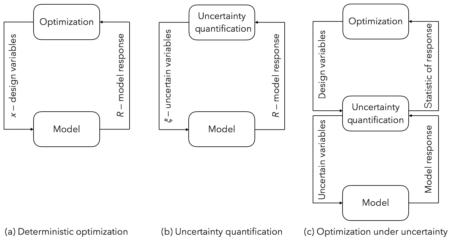
Figure 1Examples of applications that require many model evaluations. In deterministic optimization (a), we evaluate the model at different values of the design variables while searching for an optimum response. In uncertainty quantification (b), we query the model multiple times at different instances of the uncertain variables to generate an ensemble of responses from which we can compute statistics and probabilities of the model response. In optimization under uncertainty (OUU), we optimize a statistic. OUU is computationally expensive as it requires many model evaluations because of the nested loop in the problem formulation (c).
We see three approaches to improving wind farm optimization capabilities. Each approach focuses on the different blocks of the OUU problem (Fig. 1c). The first approach is to improve the modeling quality of entire wind farms, i.e., improve the models in all the disciplines (aerodynamics, structures, controls, electrical, acoustics, atmospheric physics, policy, economics, etc.) that are relevant to building and operating a wind farm, as well as the interaction between the different turbines. The second approach is to improve the optimization problem formulation and the algorithms to solve the optimization. And the third approach is to improve the treatment of the stochastic nature of the problem, i.e., develop better uncertainty quantification methods to efficiently compute the relevant wind farm statistics (and their gradients with respect to the design variables of the problem) used in the OUU problem.
The first approach increases the fidelity of the model, whereas the second (optimization) and third (uncertainty quantification) approaches seek to reduce the number of model evaluations, as this enables the study of larger and more realistic problems.
Here, we focus on the uncertainty quantification approach (the third approach), as it has not been considered in detail before. The most recent and thorough review of the wind farm optimization literature (Herbert-Acero et al., 2014) does not mention it. It only mentions the first two approaches. In the existing work in the literature, the third approach typically focuses on simple integration methods to compute the statistics, which quantify the effect of the stochastic inputs (Kusiak and Song, 2010; Kwong et al., 2012; Chowdhury et al., 2013; Fleming et al., 2016; Gebraad et al., 2017). Simple integration methods, such as the rectangle rule, are inefficient in the number of samples (simulations of the model) needed to accurately estimate a statistic, such as the AEP. They are especially inefficient if multiple stochastic inputs are considered simultaneously. Normally only the wind direction and/or the wind speed are considered stochastic input variables. Recent work (Padrón et al., 2016; Murcia et al., 2015) is starting to move beyond these simple integration techniques to compute the AEP and instead use the uncertainty quantification method of polynomial chaos to compute the AEP.
In this paper, which is meant as a comprehensive introduction to uncertainty quantification methods applied to wind farm simulations, we describe in detail the polynomial chaos (PC) method and show that, for the efficient (small number of model simulations) computation of the AEP, the PC method based on regression should be used. An additional benefit of the PC method is that it makes it feasible to consider multiple uncertain variables (e.g., wind direction, wind speed, wind turbulence, wake model parameter) that impact the computation of the AEP. An example in which a wake model parameter is considered an uncertain variable in addition to the wind speed and wind direction can be found in Padrón (2017). In addition, the PC method can be used to efficiently compute the gradient of statistics, such as the AEP. Eldred (2011) describes how to compute the gradients for PC based on quadrature. Here we show how to compute the gradients for PC based on regression (Sect. 4.3). The use of gradients allows us to efficiently tackle much larger optimization problems (Gebraad et al., 2017). To compute the gradients of the wake model, we use the recently developed Floris wake model with the modifications by Thomas et al. (2017) that provide analytic and continuous gradients of the wake model.
We first discuss the details of computing the power and the AEP of a wind farm in Sect. 2. Then, we discuss uncertainty quantification in Sect. 3 and the polynomial chaos method in Sect. 4. Finally, we discuss the details of the problem formulation in Sect. 5 and the results in Sect. 6.
We first describe the aerodynamic wake model we use (Sect. 2.1). The wake model gives an estimate of the hub-height velocity at each wind turbine, from which we can compute the power produced by the wind farm (Sect. 2.2). Then, to obtain the annual energy production (AEP) we need to integrate the power over all wind conditions that occur in a year (Sect. 2.3) and weigh the results proportionally to the frequency with which such wind conditions manifest themselves.
2.1 Floris
The Floris (FLow Redirection and Induction in Steady-state)1 (Gebraad et al., 2016) wake model is an enhancement of the Jensen wake model (Jensen, 1983) and the wake deflection model presented in Jiménez et al. (2009). The Floris model builds on the Jensen model by defining three separate wake zones with differing expansion and decay rates (controlled by tunable coefficients) to more accurately describe the velocity deficit across the wake region. A simple overlap ratio of the area of the rotor in each zone of each shadowing wake to the full rotor area is used to determine the effective hub velocity of a given turbine. A simple overview of the Floris model, showing the zones and overlap areas, is shown in Fig. 2. We use the Floris wake model with changes to remove discontinuities and add curvature to regions of nonphysical zero gradient to make the model more suitable for gradient-based optimization (Thomas et al., 2017). In this work, we use the parameter values recommended in Gebraad et al. (2016) and Thomas et al. (2017) and set the yaw-offset angle of each turbine to zero.
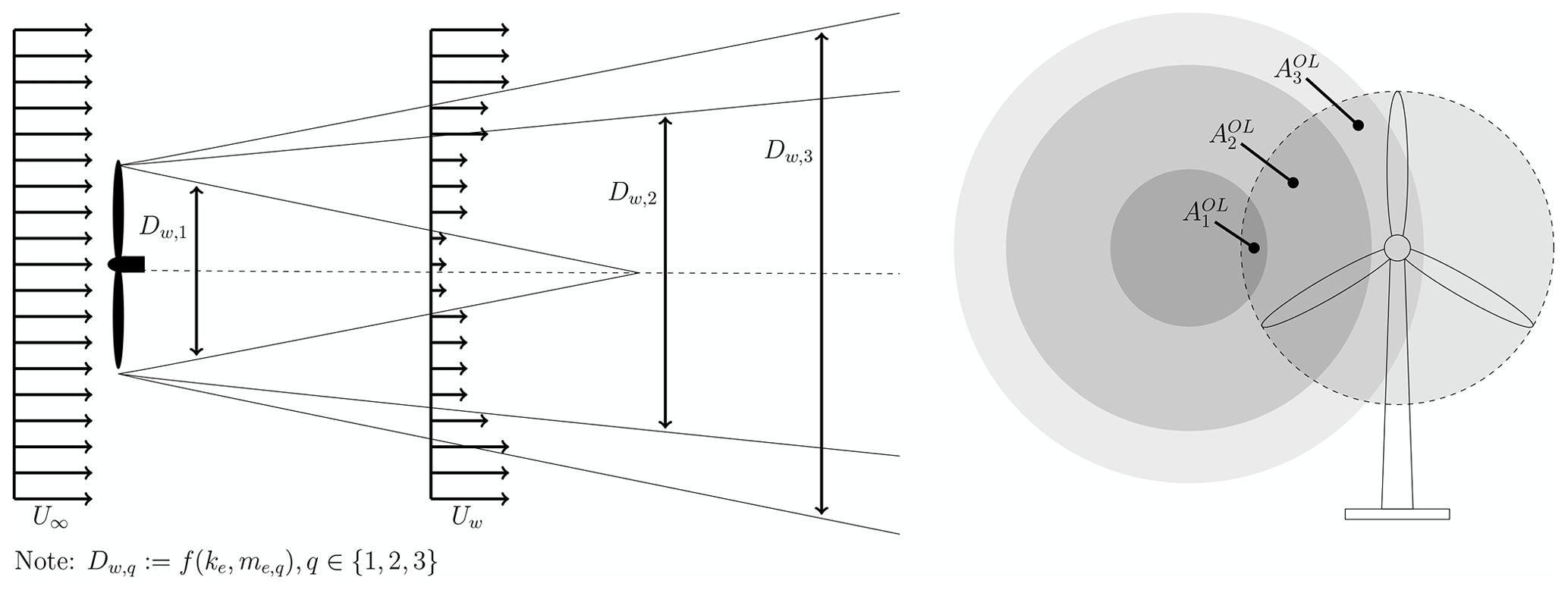
Figure 2Schematic of the Floris wake model. The model has three zones with varying diameters, Dw,q, that depend on tuning parameters ke and me,q. The effective hub velocity is computed using the overlap ratio, , of the part of the rotor-swept area overlapping each wake zone respective to the total rotor-swept area.
2.2 Computing the power of a wind farm
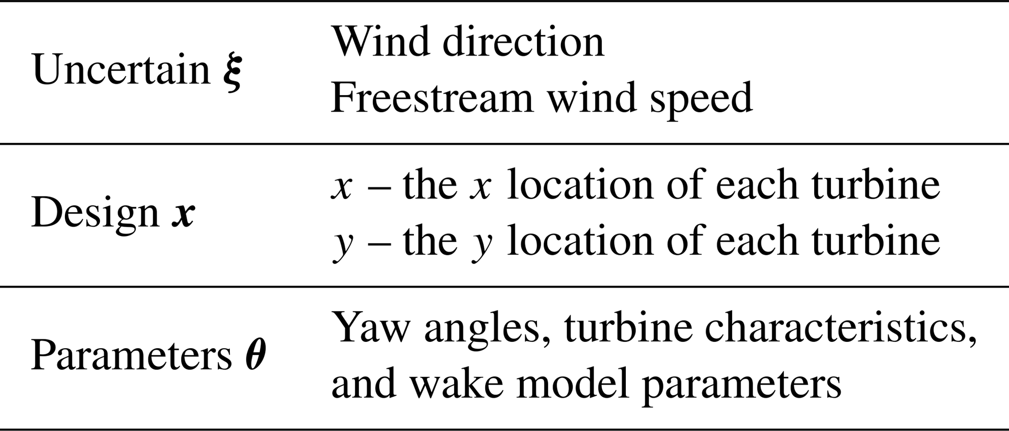
We will consider the power of the wind farm to be a function of three classes of variables: uncertain variables ξ, design variables x, and parameters θ:
Uncertain variables are variables that follow a probability distribution, design variables are variables that an optimizer can vary, and parameters are important constants that govern the behavior of the system. The classification of the variables is problem dependent. For instance, the rotor yaw could be considered a design variable, a parameter, or an uncertain variable to account for yaw-offset measurement error. A tunable parameter of a wake model, such as the wake expansion coefficient, could be considered a parameter or an uncertain variable given by a particular distribution.
For the problems considered in this work, Table 1 lists the categories into which we place each variable that influences the power computation. The uncertain variables are the wind direction and wind speed with probability distributions described in Sect. 5.1.
The power of the wind farm for a given wind direction and wind speed is equal to the sum of the power produced by each turbine . The power of each turbine is calculated from
where ρ is the air density, A is the rotor-swept area, CP is the power coefficient, and Ui is the effective hub velocity for each turbine, which is calculated by the wake model and is a function of the three types of variables described above, ). The power coefficient captures both the aerodynamic and electromechanical properties of the wind turbine. It is a complex function of many variables (Herbert-Acero et al., 2014) and is usually reported by wind turbine manufacturers as a function of the tip-speed ratio, which depends on wind speed at hub height Ui. A simple expression for CP can also be computed using the classical actuator disk theory (Sanderse, 2009).
2.3 Computing the annual energy production (AEP) of a wind farm
The annual energy production (AEP) is an important metric used to describe a wind farm. The AEP is a statistic. Specifically, it is a mean, as it is a function of the expected power multiplied by the number of hours in a year:
The expected power, E[P(ξ)], or the mean of the power, μP, is defined as
where is a vector of random variables, which we refer to as the uncertain variables, ρ(ξ) is the joint probability density function of the uncertain variables, Ω is the domain of the uncertain variables, and P is the power produced by the wind farm (Eq. 1). Common uncertain variables are the wind direction and the freestream wind speed.
The expected power, and hence the AEP, is normally computed as a weighted average, which amounts to the rectangle rule of integration (Sect. 3.1.1). Other uncertainty quantification methods (Sect. 3) can be used to compute the expected value (AEP). Specifically, we can compute the AEP efficiently by using polynomial chaos (Sect. 4).
Uncertainty quantification (UQ) is the process of (1) characterizing input uncertainties and then (2) propagating these input uncertainties through a computational model with the goal of quantifying their effect on the model's output. There are many sources of uncertainty in the modeling of a problem, and different classifications of the uncertainties have been proposed (Kennedy and O'Hagan, 2001; Oberkampf et al., 2001; Beyer and Sendhoff, 2007). A common classification is to divide the uncertainty into aleatory and epistemic uncertainties (Oberkampf et al., 2001).
In this work, we consider aleatory uncertainties that arise from the variability in the inputs to our model caused by changing environmental conditions. We describe this input variability as random variables with associated probability distributions. Thus, the first step of characterizing the input uncertainties is concerned with finding the probability distributions that describe the model's inputs. This process is known as statistical inference, model calibration, and inverse uncertainty quantification (Smith, 2014). Here, we assume that this step has been completed; i.e., we have distributions that characterize the uncertain inputs (Sect. 5.1). We focus on the second step of propagating the input uncertainties to find the statistics that describe the output.
3.1 Uncertainty propagation methods
The goal of uncertainty propagation methods is to compute the statistics that describe the effect of the uncertain inputs on the model output. There are several methods to propagate the uncertainties and compute statistics (Le Maître and Knio, 2010; Smith, 2014), and each method has its advantages and disadvantages depending on the type and size of the problem. The most common methods are sampling or Monte Carlo methods (Caflisch, 1998). Other methods include direct integration methods and stochastic expansion methods. Direct integration methods are currently used to compute the AEP of a wind farm; we briefly describe them below (Sect. 3.1.1). We describe the stochastic expansion method of polynomial chaos in detail in Sect. 4 and compare the different methods to propagate the uncertainties to compute the AEP in Sect. 6.2.
3.1.1 Direct numerical integration (rectangle rule)
As the name implies, this method numerically evaluates the integrals in the definition of the statistics. The integrals to evaluate the mean (or expected value) and the variance are
where R(ξ) is the model output and ξ the uncertain input variables. The random vector with joint probability distribution ρ(ξ) describes the input variability over the domain Ω. Each random input can follow a particular distribution ρi(ξi). For the case of independent random variables, the joint distribution is the product of each univariate distribution .
There are many quadrature methods to evaluate integrals (Ascher and Greif, 2011). We describe the rectangle rule, as this is currently used in the wind farm community to compute the AEP.
Rectangle rule
The rectangle rule, or midpoint rule, is the simplest and most straightforward quadrature method. To approximate the mean or expected value,
with the rectangle rule, we divide the domain of the uncertain variable2 into m equal subintervals of length . Next, we construct rectangles with base B=Δξ and height equal to the product of the response of the model and the density evaluated at the midpoint of the subinterval H=R(ξj)ρ(ξj). Then, the rectangle rule approximates the expected value by adding up the areas of the m rectangles:
A simple improvement is to integrate the density exactly within each subinterval:
This improvement is easily done as the density is known. This modification is helpful for a small number of evaluations m. We will use this modified rectangle rule and simply refer to it as the rectangle rule.
Polynomial chaos (PC) is the name of an uncertainty quantification (UQ) method that approximates a function with a polynomial expansion made up of orthogonal polynomials. This function has random variables as inputs, and we are interested in the effects of the random (uncertain) inputs on the output of this function. Statistics of the output can describe the effects of the inputs. We use the polynomial chaos method to efficiently compute these statistics and the gradients of these statistics.
We first describe the polynomial chaos method in Sect. 4.1. We then discuss two methods – quadrature and regression – to compute the coefficients used in the PC expansion (Sect. 4.2). In Sect. 4.3, we describe how to compute the gradients of statistics from the polynomial chaos expansion. And, in Sect. 4.4, we discuss how the PC method can be extended to include correlated random inputs.
4.1 Polynomial chaos expansion
Let R(ξ) be a function of interest that depends on the uncertain variable ξ. We can approximate the function by using a polynomial expansion:
The approximate response is a polynomial of order p. Usually, the larger the polynomial order, the closer the approximation is to the true response R(ξ).
The polynomial basis is determined by the distribution of the uncertain variable – the polynomial basis is orthogonal with a weight function that corresponds up to a constant to the probability density function of the uncertain variable. Common random (uncertain) variables (normal, uniform, exponential, beta) have corresponding classical orthogonal polynomials (Hermite, Legendre, Laguerre, Jacobi) (Eldred et al., 2008). Empirically determined distributions, such as those obtained from wind conditions, do not have corresponding classical orthogonal polynomials. For the distributions obtained from the wind conditions, we need to numerically generate custom orthogonal polynomials in order to preserve the optimal convergence property of the polynomial chaos expansion (Oladyshkin and Nowak, 2012). Details about the numerical generation of orthogonal polynomials can be found in Gautschi (2004) and an example of the generation of orthogonal polynomials for wind distributions in Padrón (2017). In addition to the optimal convergence properties, the use of orthogonal polynomials allows us to analytically compute statistics from the polynomial chaos expansion (Sect. 4.1.1).
In addition to the orthogonal polynomials, the other component of the expansion Eq. (11) is the coefficients αi. The coefficients can be computed either by quadrature or regression as described in Sect. 4.2.
For the case of multiple uncertain variables and using a multi-index , we write the multidimensional polynomial approximation as
The multidimensional basis functions Φi(ξ) are given by products of the one-dimensional orthogonal polynomials:
When the uncertain variables are independent, the multidimensional basis functions are also orthogonal (Sect. 4.4). The values of the elements ij of the multi-index depend on how the expansion is truncated, i.e., on how the index set ℐp is defined. There are two common ways in which to define the index set: total-order expansion and tensor-product expansion.
In total-order expansion a total polynomial-order bound p is enforced:
which for an expansion of total-order p with n uncertain variables results in an expansion with terms.
In tensor-product expansion a per-dimension polynomial-order bound pj is enforced:
which results in an expansion with terms.
An example showing the multidimensional basis polynomials, Eq. (13), for both the total-order expansion and tensor-product expansion can be found in Padrón (2017).
Note that for both total-order expansion and tensor-product expansion the number of terms exhibits an exponential increase with an increase in the number of uncertain dimensions n. This result is known as the curse of dimensionality. The tensor-product expansion is the preferred approach when the coefficients are computed with quadrature (Sect. 4.2.1) because of increased monomial coverage and accuracy (Eldred and Burkardt, 2009). The total-order expansion is the preferred approach when the coefficients are computed with regression (Sect. 4.2.2) because it keeps the sampling requirements lower (Eldred and Burkardt, 2009).
4.1.1 Mean and variance from the polynomial chaos expansion
The mean and variance of the function of interest R(ξ) are a function of the coefficients αi of the polynomial chaos expansion. The statistics are obtained by substituting the polynomial chaos expansion Eq. (12) into the definitions of the mean Eq. (5) and variance Eq. (8), and by integrating the expansion and simplifying using the orthogonality of the polynomials.
The mean is the zeroth coefficient,
and the variance is the sum of the product of the square of the coefficients – excluding the zeroth coefficient – with the inner product :
where the inner product is defined as and 0 is the first multi-index – the one with all zero elements.
4.2 Calculating polynomial chaos coefficients
The coefficients of the polynomial chaos expansion Eq. (12) can be calculated via quadrature or by linear regression.
4.2.1 Quadrature
To obtain the coefficients of the polynomial chaos expansion,
via quadrature, we take the inner product of both sides of Eq. (18) with respect to Φj(ξ) to yield
Making use of the orthogonality of the polynomials and solving for the coefficients in Eq. (19), we obtain
where the domain Ω is the Cartesian product of 1D domains Ωj for each dimension, , and is the joint probability density of the stochastic parameters. The inner product is known analytically or inexpensively computed. Thus, most of the computational expense in solving for the coefficients resides in evaluating the model R(ξ) in the multidimensional integral ∫ΩR(ξ)Φi(ξ)ρ(ξ) dξ. This integral is solved with quadrature (numerical integration). Note that the zero coefficient in Eq. (20) reduces to the definition of the mean:
which the direct numerical integration methods attempt to compute directly (Sect. 3.1.1).
4.2.2 Regression
To obtain the coefficients of the polynomial chaos expansion Eq. (12) via regression, we construct a linear system,
and solve for the coefficients α that best represent a set of responses R. The set of responses is generated by evaluating the model at m realizations of the uncertain vector ξ. The m uncertain vectors are most commonly obtained by sampling the density of the uncertain variables (Hosder et al., 2007).
Each row of the matrix Φ contains the orthogonal polynomials Φj evaluated at a sample ξi:
The size of the m×n matrix is determined by the number of samples m and by how the polynomial chaos expansion is truncated (Sect. 4.1), which results in n terms. It is common to specify a total-order expansion along with a collocation ratio to determine the number of samples m. The collocation ratio determines if the system is overdetermined cr>1 or underdetermined cr<1.
For overdetermined systems, the most popular method (and the one we use) to estimate the coefficients is least squares, in which we pick coefficients that minimize the residual sum of squares:
For underdetermined systems, solving a regularized least-squares problem is preferred (Doostan and Owhadi, 2011).
For a given number of samples m in the linear system Eq. (23) we can use cross-validation (Hastie et al., 2009) to pick the best polynomial-order n to approximate the response.
4.3 Gradients of statistics with polynomial chaos
Let R(ξ,x) be a function of interest that depends on uncertain variables ξ and also on design variables x. We assume independence between the design and uncertain variables3. Now the polynomial chaos expansion – over the uncertain variables – becomes
This expansion is only valid for a particular design vector – the coefficients αi(x) are a function of the design variables. Therefore, the statistics are also a function of the design variables. Specifically, the mean and the variance are
4.3.1 Gradients of the statistics with polynomial chaos
We want to know the gradients of the statistics with respect to the design variables, and we proceed to derive them below. For simplicity, we drop the subscript from the statistics μR=μ, the explicit variable dependence , the bolded notation, and we use the following notation for the gradient .
The gradient of the mean from Eq. (26) is
and the gradient of the variance from Eq. (27) is
Both the mean and the variance gradients depend on the gradient of the coefficients .
4.3.2 Gradients of the coefficients
The gradient of the coefficients can be computed with quadrature or regression, similarly to how the coefficients can be calculated with quadrature (Sect. 4.2.1) or regression (Sect. 4.2.2).
Quadrature
We start from the equation for the coefficients Eq. (20) and take the gradient to obtain
Replacing this equation into the gradient of the mean Eq. (28) we obtain
And replacing Eq. (30) into the gradient of the variance Eq. (29) we obtain
To obtain the gradients of the statistics with respect to each design variable we need to evaluate the multidimensional integral containing . The integral is evaluated with quadrature (Sect. 4.2.1) and requires the computation of the gradient of the response at each of the quadrature points. Ideally, one would use adjoint methods (Giles and Pierce, 2000) or algorithmic differentiation (Griewank and Walther, 2008) to compute the gradients, , efficiently.
Regression
We start from the linear system Eq. (22) and take the gradient to obtain the following.
To solve for the gradient of the coefficients, we solve the linear system one column at a time of the matrix with the corresponding column of the matrix of the gradients . The linear system for the multiple right-hand sides can be solved with the methods described in Sect. 4.2.2.
Again, the gradient of the mean Eq. (28) and the gradient of the variance Eq. (29) are a function of the gradient of the coefficients. Thus, to obtain the gradient of the mean, take the first row of the matrix, and for the gradient of the variance use the gradient of the coefficients from all the other rows.
4.3.3 Gradients of the statistics by direct numerical integration
Similarly to computing the mean and variance with direct numerical integration (Sect. 3.1.1), we can also compute the gradients of the mean and variance directly with numerical integration by differentiating the definitions of the mean, Eq. (5), and the variance, Eq. (8).
4.4 Correlated random variables
As described, the polynomial chaos method assumes that the uncertain variables are statistically independent. In wind farm layout optimization, the uncertain variables of wind speed and wind direction are usually correlated. There are different approaches to use polynomial chaos for problems with inputs made up of correlated (dependent) random variables. One approach is to perform a (linear or nonlinear) variable transformation (Feinberg and Langtangen, 2015) to uncorrelate the variables before applying polynomial chaos. Another approach is to construct polynomials that are orthogonal to the multivariate distribution instead of orthogonal polynomials for each dimension (Navarro et al., 2014). A third approach, which is the most applicable for the wind farm layout optimization problem, consists of breaking up the domain of the uncertain variables into smaller domains (elements) and then constructing a polynomial chaos expansion for each of the small domains and combining them in a piecewise manner to cover the whole domain. This approach of breaking up the domain is known as multielement polynomial chaos (Wan and Karniadakis, 2006). In the context of the wind farm layout optimization problem, the new distributions for the uncertain variables in the small elements can be considered independent. For example, the wind direction and wind speed at a particular wind farm site are usually correlated, but if the wind direction domain is broken into sectors, it can be assumed that within each sector the wind direction and wind speed are independent (Herbert-Acero et al., 2014; Murcia et al., 2015).
Here, we describe the details of computing AEP in the wind farm. We first describe and discuss the inputs, which are the wind direction and wind speed (uncertain variables) (Sect. 5.1), as well as the wind turbine positions (design variables) (Sect. 5.2). Then, we describe details about the output, the average AEP error (Sect. 5.3), that we use to compare the different methods we consider to compute the AEP (Sect. 5.4).
5.1 Probability distributions of the uncertain wind conditions
We consider the wind direction and the wind speed as uncertain variables with probability distributions shown in Fig. 3. The distributions show the likelihood of a particular wind direction or wind speed occurring during a year. For simplicity, we assume that the wind direction and wind speed distributions are independent (Sect. 4.4). We construct the independent distributions starting from the wind measurements taken near the Princess Amalia wind farm (Sect. 5.2) by the NoordZeeWind meteorological mast during a year (Brand et al., 2012). For a wind rose of the measurements, see Gebraad et al. (2017). The wind rose has a wind direction bin width of 5∘ and a wind speed bin width of 1 m s−1 throughout the operational range of the turbine.

Figure 3The uncertain variable probability distributions. The vertical lines show the cut-in and cut-out speed of a single wind turbine.
We construct the wind direction distribution (Fig. 3a) by linearly interpolating the wind measurements of the likelihood of the wind coming from a particular binned wind direction for all wind speeds. The zero degree direction is set at north and increases clockwise.
For the wind speed, instead of linearly interpolating the data, we fit a Weibull distribution4 and then truncate it5 (Fig. 3b). We truncate the distribution to correspond to the operational range of the turbine from the cut-in speed of 3 m s−1 to the cut-out speed of 25 m s−1.
The probability distributions are the weight functions of the orthogonal polynomials used in the polynomial chaos method (Sect. 4.1). For both of the distributions (weight functions), we use a histogram of 50 equal width bins to describe each distribution. Using these weight functions, we then numerically generate their corresponding orthogonal polynomials.
5.2 The wind farm layouts
To showcase the results, we will focus on four representative layouts: Grid, Amalia, Optimized, and Random (Fig. 4). Each layout has 60 turbines, and in the figures each turbine is represented by a dot to scale – the diameter of the dot represents the rotor diameter. The Grid layout fits in a box of equivalent area to that of the Amalia layout. The Amalia layout, which is grid-like, is that of the Princess Amalia wind farm located 23 km off the coast of the Netherlands. The Optimized layout is a representative optimal layout obtained by running the optimization problem (Sect. 6.3.1); specifically, it is the layout shown in Fig. 11a. When we refer to this particular optimized layout, we will capitalize the word optimized. The Random layout was generated by random sampling and keeping the turbines that are contained within the convex hull of the Amalia wind farm while also satisfying a minimum inter-turbine spacing of three diameters. We will refer to the Grid and Amalia as grid-like layouts and the Optimized and Random as non-grid-like layouts.
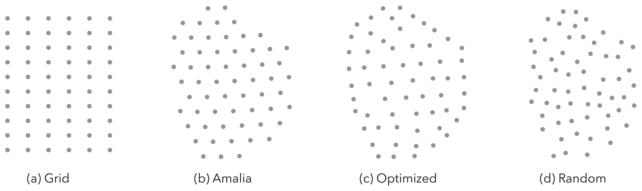
Figure 4Representative wind farm layouts used in the results. Each dot represents a wind turbine to scale – the dot represents the swept area of the rotor.
In reality, the 60 turbines in the Princess Amalia wind farm are the Vestas V80 model. For each of the layouts in our study, we use the NREL 5 MW reference turbine (Jonkman et al., 2009), as this turbine has an open-source design.
5.3 Convergence metric – the average AEP error
We use an ensemble of 10 AEP results to compute the average AEP error. The average AEP error allows us to better illustrate the differences between the different methods used to compute the AEP and to avoid drawing conclusions from one-off solutions. We found that averaging over 10 AEP results is enough to illustrate the difference between methods and to smooth out the convergence of the AEP error (Fig. 8). The ensemble of results accounts for the fact that the zero (starting) position for the wind direction is arbitrary (it could be north, south, east, west, etc.). Also, averaging the AEP errors helps smooth out the AEP convergence curves by reducing the sensitivity of the AEP to the quadrature (sample) points used to compute the AEP. We generate the ensemble of AEP results by selecting 10 different input sets. For example, for the rectangle rule, if we consider 36 wind directions the 10 sets are ; ; …; . For the polynomial chaos based on quadrature, the quadrature points are the numerically generated Gaussian quadrature points for the interval. Thus, to create 10 different sets, we pick 10 different intervals; i.e., we pick different starting positions. We set the starting positions for the intervals at ∘ for i=0…9. For both the rectangle and polynomial chaos based on quadrature, the wind speed points for each set are the same. For the polynomial chaos based on regression and for Monte Carlo, the wind directions and wind speed pairs are generated by sampling the distribution. Thus, to obtain 10 different sets, 10 different samplings are performed. We use the average AEP error as the convergence metric:
5.3.1 Baseline AEP
We take as the baseline or true AEP the AEP computed with 200 000 Monte Carlo samples. We picked 200 000 Monte Carlo samples to ensure that the 99 % confidence interval for the true AEP was smaller than 1 % of the computed AEP value for all layouts. We consider an AEP within 1 % of the baseline AEP to be accurate, and we will use it as a reference for the results. AEP predictions of real wind farms usually have an error of 10 %–20 % (Barthelmie et al., 2007; Briggs, 2013) due to uncertainty in wind conditions and the errors of wake models, and thus resolving the AEP to less than 1 % is unnecessary.
5.4 Methods to compute the AEP
Here, we provide the details of the methods used to compute the AEP and the abbreviations for the methods.
- rect
-
rectangle rule (Sect. 3.1.1)
- PC-Q
-
polynomial chaos based on quadrature (Sect. 4.2.1)
- PC-R
-
polynomial chaos based on regression (Sect. 4.2.2)
For the quadrature-based methods (rect, PC-Q), we use tensor-product quadrature to compute multidimensional integrals. We use the same number of points for each dimension because we did not see any benefit in favoring a particular dimension. For PC-Q, we use Gaussian quadrature. For Monte Carlo, we use the traditional Monte Carlo method, i.e., random samples. For PC-R, we use Latin hypercube sampling (McKay et al., 1979) to generate the samples needed to construct the linear system. We solve the linear system with least squares. For a given number of samples, given by the total polynomial order p, we use 10-fold cross-validation to find the least-squares best fit from polynomials of total order 1 up to total order p. The sampling methods and the polynomial chaos methods we use are implemented in the open-source DAKOTA toolkit (Adams et al., 2017).
We first characterize the power output of the wake model for different input conditions (Sect. 6.1). Next, we focus on the convergence of the AEP (Sect. 6.2) and then on the wind farm layout optimization problem to maximize the AEP (Sect. 6.3).
6.1 Power response as a function of the uncertain variables
The power production, computed with the Floris wake model, for the four wind farm layouts (Sect. 5.2) as a function of both the wind direction and the wind speed is shown in Fig. 5. The wind direction is measured from north and increases clockwise. The power response as a function of the wind direction is highly oscillatory, and for layouts with structure6, it is periodic. The peaks in the contour lines identify wind directions for which there is a poor performance (low power). The grid-like layouts (top row of Fig. 5) have larger peaks due to wind turbines being aligned along particular directions and thus experiencing full-wake conditions. The worst wind direction for the Grid layout is directly from north (0∘) or south (180∘) when rows of 10 turbines are aligned.
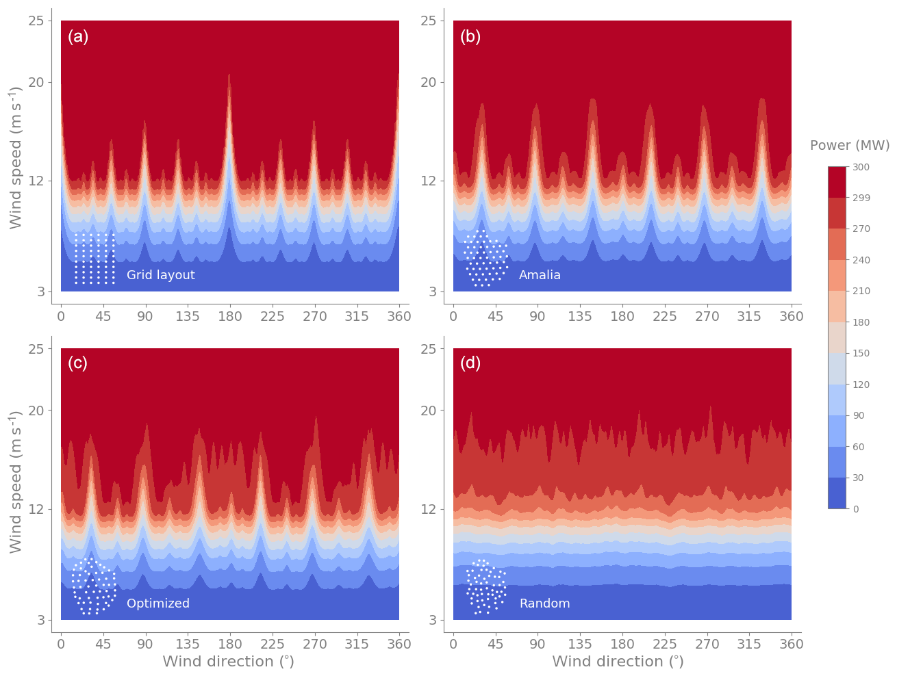
Figure 5Power contours as a function of wind direction and wind speed for the Grid, Amalia, Optimized, and Random layouts. The grid-like layouts (a, b) have larger peaks due to wind turbines being aligned along particular directions and thus experiencing full-wake conditions. For all layouts, as the speed increases the power increases until the wind farm reaches its rated power of 300 MW.
The power response as a function of the wind direction has similar shapes for different wind speeds until the speed is high enough (larger than the rated speed of the layout) that the response gets clipped at 300 MW (all 60 turbines are operating at their rated power 5 MW). As a function of the wind speed, for each wind direction, the power response starts after the cut-in speed of 3 m s−1 and is cubic (concave up) until individual turbines start reaching rated power. After that, the power increases more slowly (concave down) until the farm reaches its rated power. The less grid-like layouts show a smoother transition to the maximum power because each turbine reaches its rated speed (11.4 m s−1) at different freestream speeds.
The power response as a function of the uncertain variables (wind direction and wind speed) is a complicated function, which needs to be integrated weighted by the likelihood of the wind conditions, to obtain the AEP of the wind farm. Next, we show that using polynomial chaos instead of the rectangle rule results in better estimates of the AEP.
6.2 AEP convergence: polynomial chaos vs. rectangle rule
We consider the AEP as a function of two uncertain variables: the wind speed and the wind direction. The AEP is usually considered a function of these two variables. We compare the convergence of the AEP for the different methods to compute the AEP: polynomial chaos (based on quadrature and regression), the rectangle rule, and Monte Carlo (Fig. 6). The polynomial chaos based on regression (PC-R) performs the best for all layouts. It is followed by the polynomial chaos based on quadrature (PC-Q) and the rectangle rule, which perform similarly. The worst performer is Monte Carlo. The slow convergence of statistics with Monte Carlo is well known. Monte Carlo will start to outperform the other methods when the AEP is a function of a large number (5–10) of uncertain variables, as it does not suffer from the curse of dimensionality.
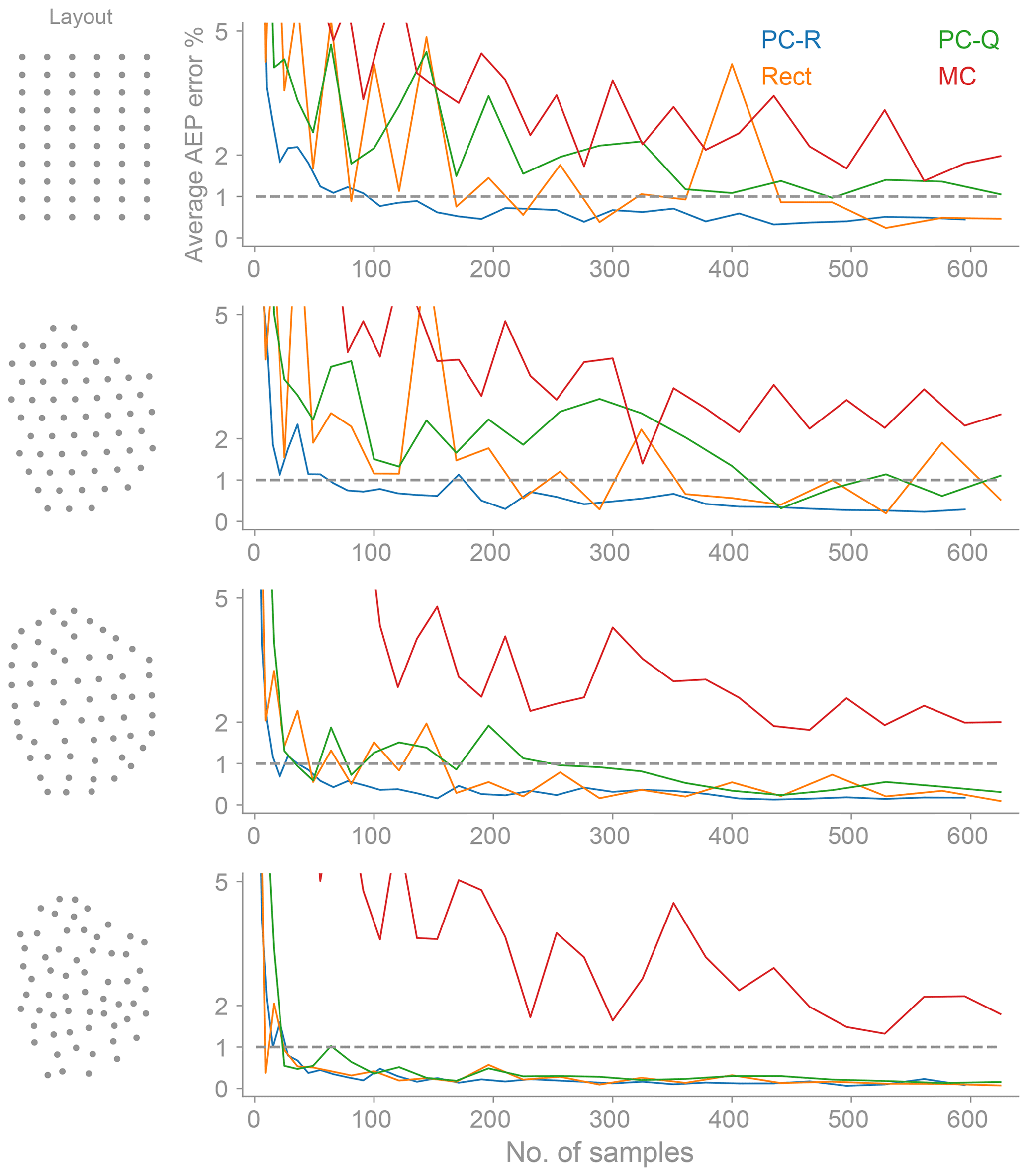
Figure 6The average AEP error as a function of the number of samples for polynomial chaos (based on regression and quadrature), the rectangle rule, and Monte Carlo. The AEP is a function of two uncertain variables: the wind direction and wind speed. The polynomial chaos based on regression performs best for all layouts.
The superior performance of the polynomial chaos based on regression, especially for the grid-like layouts (Grid and Amalia), is due to the following: the polynomial chaos fit based on regression does not chase all the high-frequency oscillations in the power response (Fig. 5); i.e., it smooths out the response. The PC-R fit is usually not higher than an 8 total-order polynomial (Sect. 4.1), whereas the PC-Q-order fit is higher, as it is directly proportional to the number of samples per dimension7. A downside of the PC-R being able to predict the mean (AEP) accurately is that it can underpredict the true variance (standard deviation) of the response (Fig. 7). Usually, the standard deviation of the power response (energy) over a year is not considered as a function to optimize. A common objective in wind farm optimization is to maximize the total amount of energy produced over a year independent of the variability in the power production over the year. For a wind farm, the variability of the energy produced over a year is less important than the variability caused by the changing wind conditions during the day.
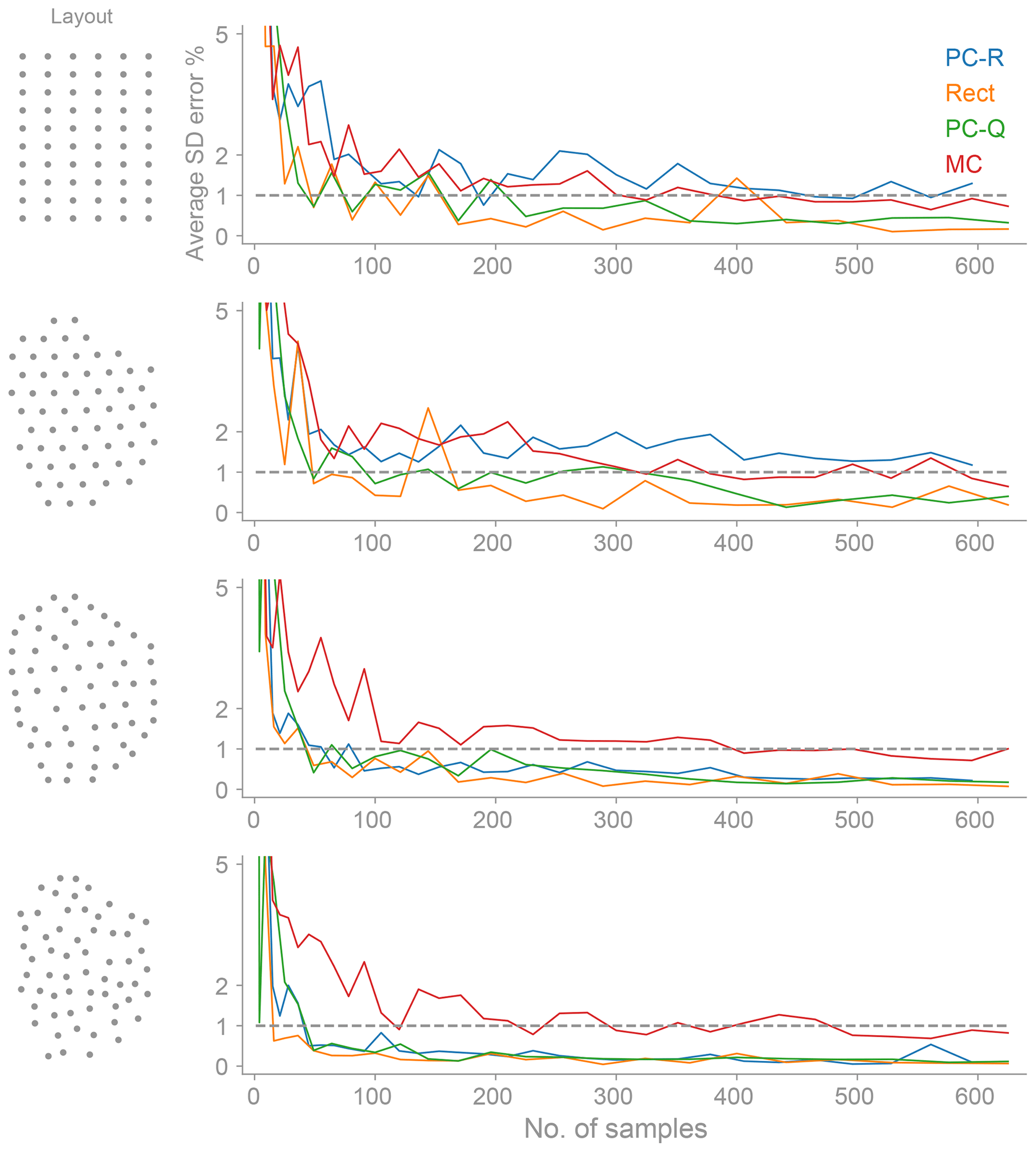
Figure 7The average standard deviation of the energy (SD) error as a function of the number of samples for polynomial chaos (based on regression and quadrature), the rectangle rule, and Monte Carlo. The SD is a function of two uncertain variables: the wind direction and wind speed. Note that the PC-R response is biased for the Grid and Amalia layouts. The PC-R underpredicts the true SD at the expense of computing the mean (AEP) more accurately (see Fig. 6).
In what follows we will compare the PC-R (the best-performing method) with the rectangle rule (the method most commonly used in practice) to quantify the reduction of samples needed to compute the AEP accurately. Also, we will sometimes use polynomial chaos to refer to polynomial chaos based on regression. Figure 8 only keeps PC-R and the rectangle rule results from Fig. 6, and, in addition, the figure shows the average AEP error computed with 10 and 100 sets of samples for each method. For the rectangle rule, there is hardly any difference between the average AEP error computed with 10 or 100 sets. For the PC-R method, the average error with 100 sets shows a smoother convergence. In general, averaging the AEP error over 10 sets of samples is enough to minimize the AEP's sample location sensitivity and to clearly see the differences between the methods used for computing the AEP (Sect. 5.3).
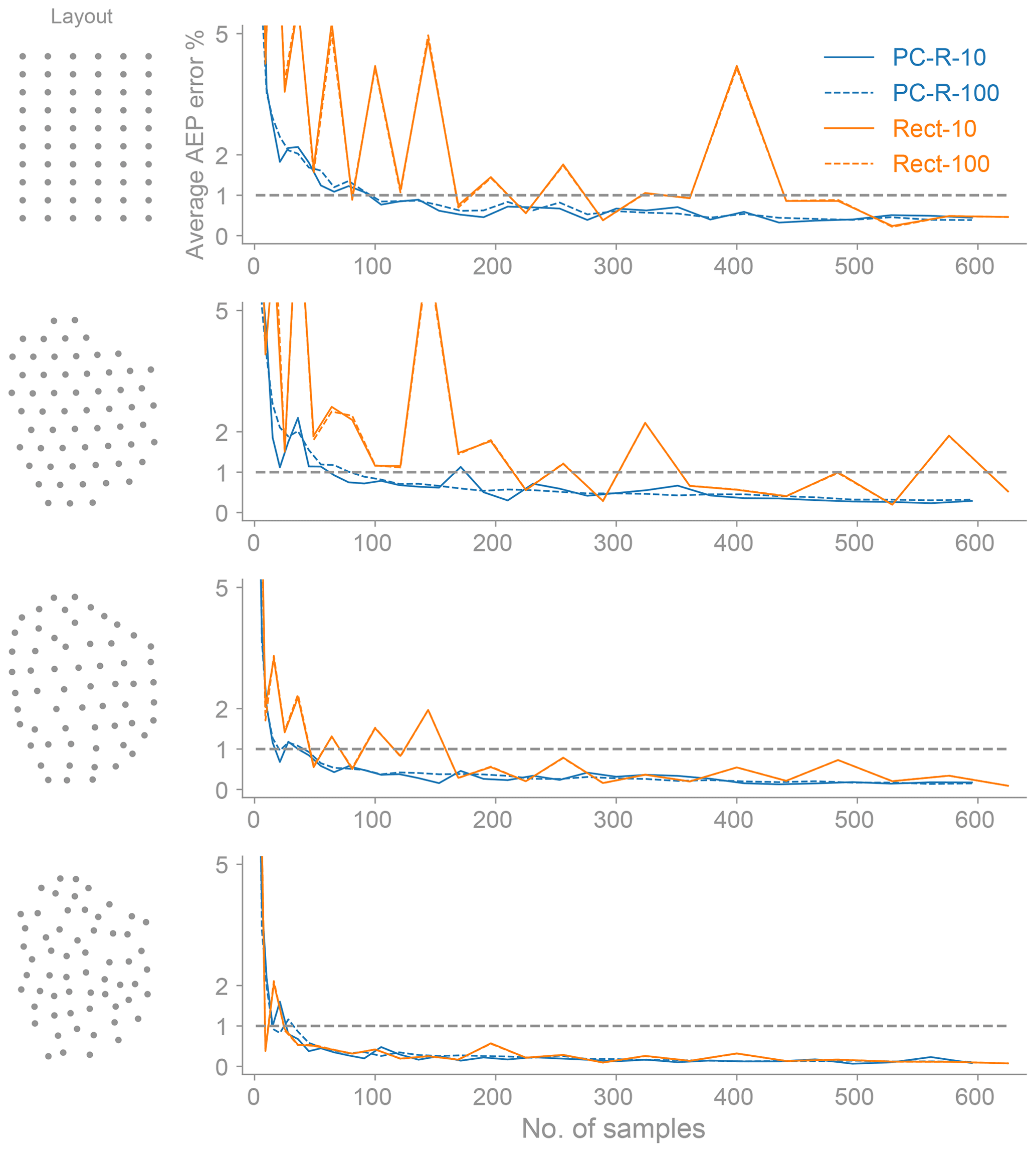
Figure 8The average AEP error as a function of the number of samples for both the rectangle rule and polynomial chaos based on regression (this is the same as Fig. 6, with only keeping the PC-R and the rectangle rule results). In addition, we show the average AEP error computed with 10 (solid line) and 100 (dashed line) sets of samples (Sect. 5.3). The AEP is a function of two uncertain variables: the wind direction and wind speed. The polynomial chaos method computes the AEP more accurately with fewer samples.
In Fig. 8, we see that the PC-R convergence curve is consistently below the rectangle rule curve; i.e., PC-R has a smaller error for the same number of samples or the same error for a smaller number of samples. Using the 1 % average AEP error as a metric, we see that PC-R achieves this error with fewer samples than the rectangle rule. The reduction in the number of samples is on the order of 4 times for the Grid layout, 8 times for the Amalia, 4 times for the Optimized, and no significant improvement for the Random. These reductions in the number of samples are considerable. In addition to providing faster convergence of the AEP, the polynomial chaos based on regression method converges the AEP more smoothly, with less oscillatory, more monotone convergence. Smooth convergence is always a desired property, and it is especially useful when performing an optimization. Both methods, PC-R and the rectangle rule, perform better for the less grid-like layouts because there is less variability in the power responses as a function of wind direction (see Fig. 5). This is beneficial, as in the first few iterations of an optimization the starting grid-like layouts become non-grid-like and start to resemble the Optimized layout.
The polynomial chaos based on regression is not only better on average, as we have seen in Fig. 8, but it is also better in general, as shown in Fig. 9. The shaded area in Fig. 9 shows the spread between the maximum and minimum AEP for 10 realizations of each of the number of samples (Sect. 5.3). The solid line shows the average of those 10 realizations and the dashed lines the ±1 % of the baseline AEP. We see that the spread is significantly smaller for the polynomial chaos based on regression and that by around 300 samples the predictions are almost always within 1 % of the true AEP for the grid-like layouts (Grid and Amalia) and around 100 samples for the non-grid-like layouts (Optimized and Random). In contrast, for the rectangle rule, the error in the AEP is still larger than 1 % at 400 samples for the Grid layout and 600 samples for the Amalia layout.
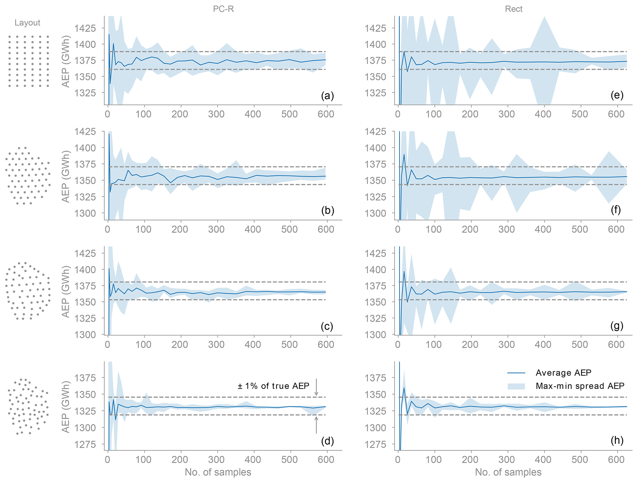
Figure 9Variability in the convergence of the AEP. Panels (a)–(d) are for polynomial chaos based on regression and panels (e)–(h) for the rectangle rule. The shaded area shows the spread between the maximum and minimum AEP for 10 realizations of each of the number of samples. The range in the plots corresponds to ±5 % of the true AEP for each layout. The variability is significantly smaller for polynomial chaos, which shows that in general it outperforms the rectangle rule. The PC-R method obtains smaller variability by smoothing out the high-frequency oscillations present in the power response (Fig. 5).
6.3 Wind farm layout optimization
6.3.1 Optimization problem
The objective of the wind farm layout optimization is to maximize the AEP (Sect. 2.3) by changing the position of the wind turbines. We assume a fixed number of turbines, 60, of the same type (NREL 5 MW; Jonkman et al., 2009) and constrain the turbines to stay within a given area and with a minimum separation between them. This objective and the constraints result in a problem of nonlinear optimization under uncertainty with deterministic constraints:
where Si,j is the distance between each pair of turbines i and j, and D is the turbine diameter. The normal distance, Ni,b, from each turbine i to each boundary b is defined as positive when a turbine is inside the boundary and negative when it is outside of the boundary. The boundary is the convex hull of the Princess Amalia layout – a 14-sided convex polygon (dashed-line boundary in the upper left of Fig. 10). The design variables are the x, y coordinates of the 60 wind turbines, resulting in 120 design variables. The uncertain variables ξ in the objective are the wind direction and wind speed.
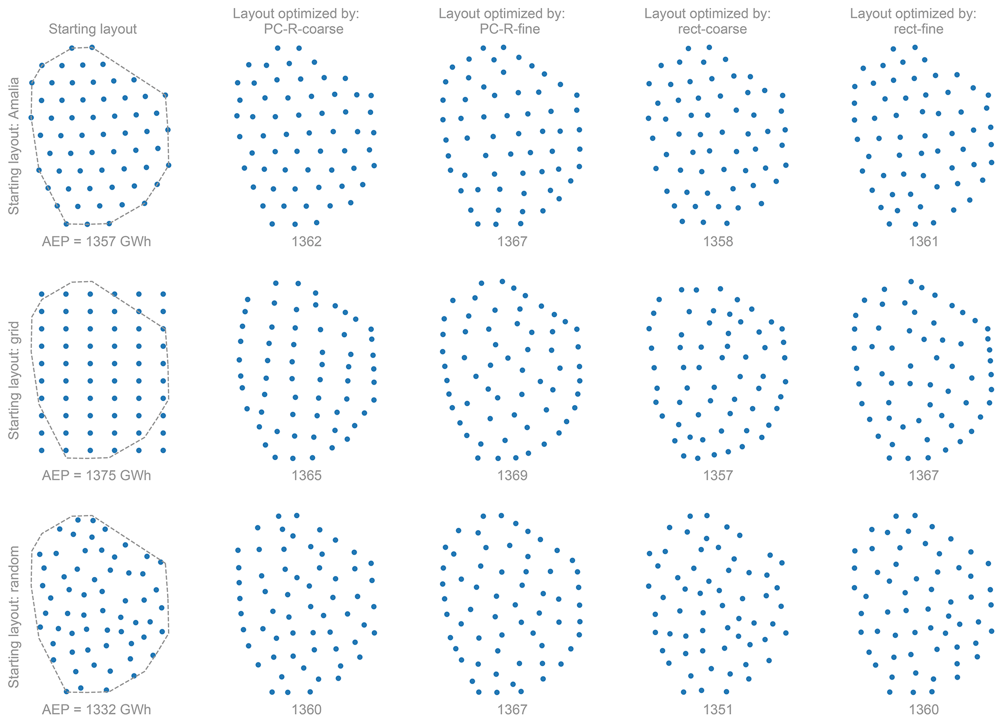
Figure 10Optimal wind farm layouts achieved for each method to compute the AEP. The layouts in the first column show the turbine starting positions for the optimization along with the boundary constraint (dashed line). The optimal layouts correspond to those with the maximum AEP from Table 2.
We solve the optimization problem with the gradient-based sequential quadratic programming optimizer SNOPT (Gill et al., 2005). We use OpenMDAO (Gray et al., 2010) and its wrapper for pyOptSparse (Perez et al., 2012) to call SNOPT from Python. We scale the variables, constraints, and the objective to make them of order 1 and set the tolerances to per the function (AEP) precision.
6.3.2 Optimization results
We solve the optimization-under-uncertainty problem, Eq. (37), using the rectangle rule and polynomial chaos based on regression methods to compute the AEP. For each method, we consider a coarse and fine number of samples to compute the AEP. Also, for each method, we run 10 optimizations, and each optimization uses different sample points to compute the AEP (see Sect. 5.3). The 10 optimizations enable us to get a better understanding of which method is better at finding layouts with high AEP and to avoid drawing conclusions from one-off local optima. Furthermore, we consider three different starting layouts for the optimization: Amalia, Grid, and Random (Sect. 5.2). The results of the optimizations are reported in Table 2.
Table 2The AEP of the optimized layouts. We generate the AEP statistics for each method from a set of 10 different optimizations. For a similar number of samples, both coarse and fine, polynomial chaos based on regression produces better optimal layouts than the rectangle rule. Furthermore, using about one-third of the samples, PC-R optima are comparable with the optima obtained with the rectangle rule that used 625 samples to compute the AEP. The values of the AEP reported are computed with 200 000 Monte Carlo samples.
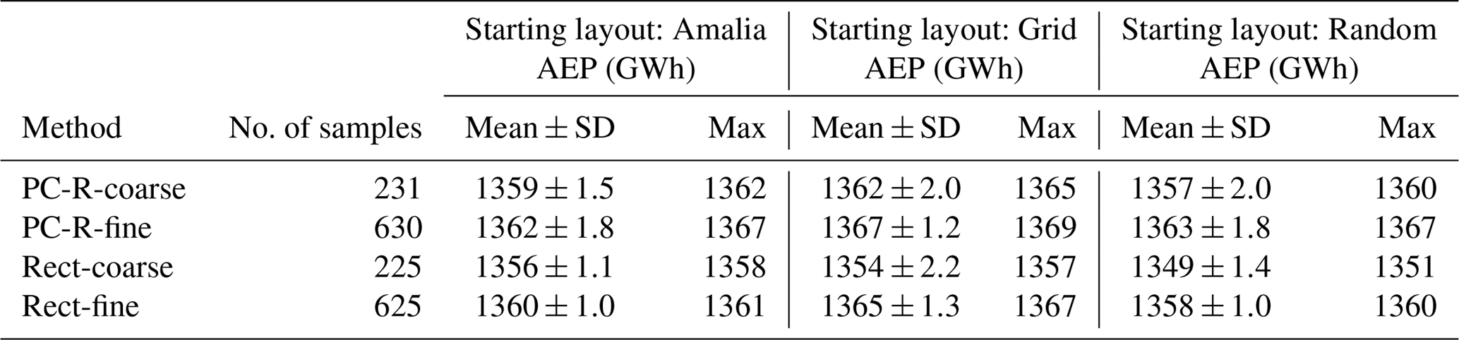
The optimum layouts obtained with polynomial chaos based on regression are better than those obtained with the rectangle rule. For a similar number of samples to compute the AEP, the optimizations with polynomial chaos produce on average optimal layouts with 0.4 % higher AEP than the optimizations with the rectangle rule. Also, using about one-third of the samples, the optima obtained with polynomial chaos are comparable to those obtained with the rectangle rule. Furthermore, polynomial chaos finds better local optima than the rectangle rule for all the different starting layouts considered (Table 2).
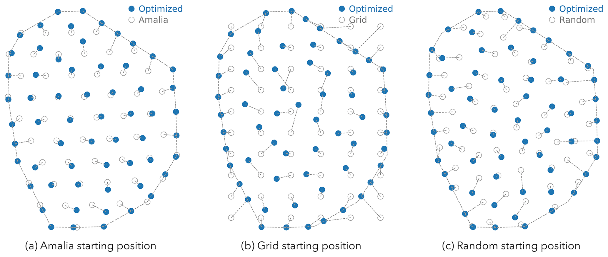
Figure 11The initial and optimized position of the turbines for the layouts obtained with the PC-R-fine method from Fig. 10. To minimize wake losses, the turbines try to spread out as much as possible and position themselves at the boundary of the layout.
The optimal layouts with the maximum AEP for each method and starting layout are shown in Fig. 10. As can be seen in that figure, the wind farm layout optimization problem contains many local optima. In general, the turbines – in the local optima – position themselves in non-grid-like patterns to minimize wake losses. Also, to minimize wake losses, the turbines try to spread out as much as possible and position themselves at the boundary of the layout (Fig. 11). For the optima obtained starting from the Amalia layout, we see that the distribution of the turbines is somewhat similar to the starting layout. As the Amalia layout is already a good layout8, it is not surprising that the local optima somewhat resemble the Amalia layout. The optima found starting from the Grid layout have on average the highest AEP (Table 2 and Fig. 10). When considering all methods, on average, the optimal layouts found starting from the Grid layout are 0.2 % higher than the optimal layouts starting from the Amalia layout and 0.4 % higher than the optimal layouts starting from the Random layout. The Grid layout is infeasible, as many of the turbines do not satisfy the boundary constraint (Fig. 11). However, starting from the infeasible layout is beneficial as it nudges the turbines to position themselves on the boundary. The optima found starting from the Random layout have on average the lowest AEP, but they have the most improvement in AEP over the starting layout, showing that we can find a good layout even from a poor starting position (Fig. 12). Due to the presence of many local optima, starting from a good layout will usually find layouts that are better than those starting from a bad layout, such as the Random.
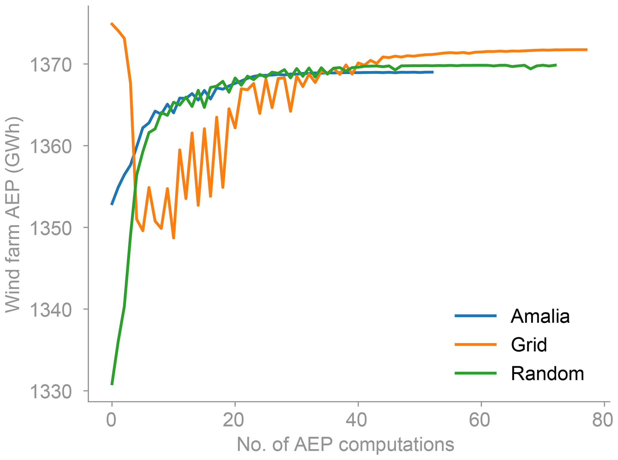
Figure 12Convergence history of the optimization for the different starting layouts. The convergence history is for the layouts in Fig. 11.
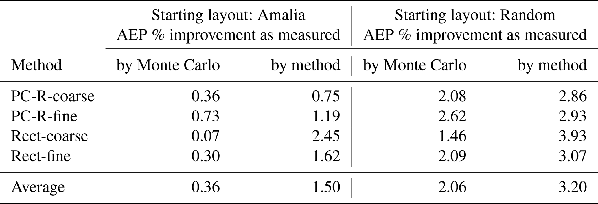
To properly compare the results obtained by the different methods used to compute the AEP in the optimization, we should compute the AEP of the optimal layout with a method that was not used in the optimization. The values of the AEP reported in Table 2 and Fig. 10 are computed with 200 000 Monte Carlo samples. For consistency, and to avoid potential uncertainty in the results introduced by the sample locations, we use the same 200 000 samples – wind direction, wind speed pairs – to evaluate the optimal layouts obtained by each method. Using the AEP computed with Monte Carlo, the improvement of the optimal layout over the starting layout will in general be lower than the improvement in AEP as measured by the method used in the optimization (Table 3). For example, for the optimal layouts in Fig. 10, with the Amalia starting layout, the average improvement in AEP over the starting layout for all the methods is 0.36 % when measured with the Monte Carlo samples and 1.50 % when measured by using the method used in the optimization. For the optimizations starting from the Random layout, the average AEP improvements are 2.06 % for Monte Carlo and 3.20 % for the method used in the optimization. As the optimizations starting from the Grid layout are infeasible, we do not include the improvement in AEP for the Grid layout in Table 3. The improvements we have found starting from the Amalia layout are similar to those found by Gebraad et al. (2017) for turbine position optimization.
Table 3The improvement in AEP of the optimized layouts from Fig. 10 over their starting layouts. The improvements are smaller when measured by 200 000 Monte Carlo samples rather than directly by the method used to compute the AEP in the optimization.
Most optimizations required on the order of 100 AEP computations. The optimization history for the layouts in Fig. 11 is shown in Fig. 12. Note that each AEP computation requires hundreds (the number of samples specified for each method in Table 2) of calls to the wake model, resulting in tens of thousands of calls to the wind farm wake model per optimization. If the gradients of the AEP are computed with a first-order finite difference, 120 (the number of design variables) times as many wind farm wake model calls would be needed per optimization. We showed that using polynomial chaos finds comparable optima to the rectangle rule but using only about one-third of the samples per AEP computation. Thus, polynomial chaos finds comparable optima for roughly one-third of the optimization computational cost. And, for the same computational cost, polynomial chaos produces optimal layouts with 0.4 % higher AEP on average.
A single wind farm layout optimization requires tens to hundreds of thousands of model evaluations. During the design phase of a new wind farm, designers need to perform many optimizations. The designers may explore scenarios with different turbine types, different sites, larger farms with a different number of turbines, and possibly even systems of wind farms. Also, the presence of local optima would require many optimizations with different restarts to find the best layout. And, furthermore, there is a desire to increase the fidelity of the models used to simulate the wind farm, which will increase the time and computational cost of the optimizations9. Thus, to facilitate the design phase of new wind farms and to incorporate the use of higher-fidelity models in the design phase requires significant improvements to reduce the simulation requirements (computational cost) of performing the wind farm problem of optimization under uncertainty (OUU) (Fig. 1c).
We proposed the use of polynomial chaos (PC) to improve the uncertainty quantification step of the OUU problem. We computed AEP convergence plots and showed that polynomial chaos based on regression (PC-R) could compute the AEP accurately using on average one-fifth of the simulations required using the rectangle rule, the method currently used in practice in the wind industry. PC-R computes the AEP accurately (error less than 1 %), usually with only 200 simulations or fewer depending on the wind farm layout – a significant improvement over the current industry practice of using more than 1000 model evaluations to compute the AEP.
The layout of the wind farm influences the convergence of the AEP because the layout has a significant effect on the power output of the farm as the wind conditions vary (Fig. 5). We considered four representative layouts: Grid, Amalia, Optimized, and Random. The power response of the grid-like layouts (Grid and Amalia) has large oscillations caused by the large drops in power that occur when rows of wind turbines are aligned with particular wind directions. Because of the larger variability in the power response, the grid-like layouts require more simulations than the non-grid-like layouts (Optimized and Random) to converge the AEP. An extension of this work that could potentially further improve the convergence of the AEP, especially for the grid-like layouts, would be to build an approximation to the power output that takes into consideration the oscillatory and periodic behavior of the wind farm response with respect to the wind direction (Fig. 5): for instance, by using Fourier series to approximate the wind direction response and polynomials for the wind speed response.
In addition to computing the AEP efficiently, a benefit of using polynomial chaos is that it can also compute the gradient of the AEP efficiently. The use of gradients is essential to enable large-scale wind farm optimization. We described how to compute the gradients of the AEP in Sect. 4.3. A benefit of using the rectangle rule is that no special consideration is necessary for correlated uncertain variables, whereas for polynomial chaos, some extra considerations are necessary as discussed in Sect. 4.4. Another benefit of using PC is that it can easily incorporate multiple-fidelity models to accelerate the convergence of statistics (Ng and Eldred, 2012; Palar et al., 2016), such as the AEP (Padrón, 2017). Furthermore, the effect of other uncertain variables (such as wake model parameters) on the AEP can easily be incorporated in the polynomial chaos framework. As the number of uncertain variables increases, polynomial chaos based on regression will continue to outperform the rectangle rule (see Padrón, 2017, for an example with three uncertain variables – wind speed, wind direction, and wake model parameter). For a large number (5–10) of uncertain variables, the Monte Carlo method will start to outperform polynomial chaos because it does not suffer from the curse of dimensionality (Smith, 2014).
We performed multiple gradient-based wind farm layout optimizations to compare the optimization results obtained with the different methods to compute the AEP: polynomial chaos based on regression and the rectangle rule. The goal of the optimization was to maximize the annual energy production (AEP) of the wind farm. The layout optimization is an OUU problem (Fig. 1c) with the wind speed and wind direction as uncertain variables and the positions of the wind turbines as design variables. In the resulting optimal layouts, the turbines position themselves in non-grid-like patterns and spread toward the boundary to minimize wake losses. For the optimization problem posed, there are many local optima with different patterns and similar AEP (Fig. 10). To search for the best optimum, we considered different starting layouts (Grid, Amalia, and Random). We observed that starting from a good layout (Grid, Amalia) will, in general, find better optima than starting from a bad layout (Random) independent of the method used to compute the AEP.
An ensemble of optimizations should be used to properly compare the optimal layouts obtained using the different methods to compute the AEP. Also, for proper comparison, the AEP of the optimized layouts should be evaluated in the same way and with a method different from the one used in the optimization. To be confident about the differences between the optimal layouts, we evaluated the AEP of each optimized layout using the same 200 000 Monte Carlo samples. We found that the benefits of being able to efficiently compute the AEP with PC-R translate to being able to find better optima than those obtained when computing the AEP with the rectangle rule when using the same number of simulations. For the cases considered, on average, with PC-R we find optima that are 0.4 % better than those found with the rectangle rule. This is a significant improvement, as a 1 % increase in the AEP for a modern large wind farm can increase its annual revenue by millions of dollars. Also, using about one-third of the simulations, coarse PC-R finds comparable optima to those found by using the fine rectangle rule for the optimization cases considered.
An interesting extension of this work that could further improve the AEP would be to allow yaw-based control in the optimization problem to take advantage of wake deflection. Gebraad et al. (2017) found that including yaw for each wind direction in a secondary layout optimization, after layout optimization without yaw, resulted in an additional 3.7 % increase in AEP. Including wake deflection in the wind farm layout optimization increases the complexity of the problem in terms of the number of design variables because every wind direction (and, to a lesser extent, wind speed) calls for different yaw values for each turbine. The increased number of design variables makes the problem much more difficult for gradient-free optimization methods and can slow down gradient-based optimization methods as well (Thomas et al., 2017). As we have seen, polynomial chaos reduces the number of simulations (wind directions and wind speeds considered). Thus, it could also greatly reduce the number of simulations in optimization with yaw control.
Data are available at https://doi.org/10.5281/zenodo.2667424 (Padrón et al., 2019).
ASP performed the investigations and wrote the article. All authors reviewed and edited the manuscript. JT assisted with the wake model. JT and APJS assisted with setting up the optimization problems. AN and JJA provided direction and supervision for the entire project.
The authors declare that they have no conflict of interest.
Funding for this research was provided by the National Science Foundation under a collaborative research grant (nos. 1539384 and 1539388).
This paper was edited by Johan Meyers and reviewed by three anonymous referees.
Adams, B. M., Ebeida, M. S., Eldred, M. S., Jakeman, J. D., Swiler, L. P., Stephens, J. A., Vigil, D. M., Wildey, T. M., Bohnhoff, W. J., Dalbey, K. R., Eddy, J. P., Hu, K. T., Bauman, L. E., and Hough, P. D.: Dakota, a multilevel parallel object-oriented framework for design optimization, parameter estimation, uncertainty quantification, and sensitivity analysis: version 6.6 user's manual, Tech. rep., Sandia National Laboratories, Albuquerque, New Mexico, USA, 2017. a
Ascher, U. M. and Greif, C.: Chapter 15: numerical integration, in: A First Course Numer. Methods, 441–479, SIAM, Philadelphia, PA, https://doi.org/10.1137/9780898719987.ch15, 2011. a
AWEA: AWEA U.S wind industry annual market report year ending 2015, Tech. rep., American Wind Energy Association, available at: https://www.awea.org/resources/publications-and-reports/market-reports/2015-u-s-wind-industry-market-reports (last access: 28 April 2019), 2016. a
Barthelmie, R. J., Frandsen, S. T., Nielsen, M. N., Pryor, S. C., Réthoré, P. E., and Jørgensen, H. E.: Modelling and measurements of power losses and turbulence intensity in wind turbine wakes at middelgrunden offshore wind farm, Wind Energy, 10, 517–528, https://doi.org/10.1002/we.238, 2007. a, b
Barthelmie, R. J., Hansen, K., Frandsen, S. T., Rathmann, O., Schepers, J. G., Schlez, W., Phillips, J., Rados, K., Zervos, A., Politis, E. S., and Chaviaropoulos, P. K.: Modelling and measuring flow and wind turbine wakes in large wind farms offshore, Wind Energy, 12, 431–444, https://doi.org/10.1002/we.348, 2009. a
Belu, R. and Koracin, D.: Statistical and spectral analysis of wind characteristics relevant to wind energy assessment using tower measurements in complex terrain, J. Wind Energy, 2013, 1–12, https://doi.org/10.1155/2013/739162, 2013. a
Beyer, H. G. and Sendhoff, B.: Robust optimization – a comprehensive survey, Comput. Method. Appl. M., 196, 3190–3218, https://doi.org/10.1016/j.cma.2007.03.003, 2007. a
Brand, A., Wagenaar, J., Eecen, P., and Holtslag, M.: Database of measurements on the offshore wind farm Egmond aan Zee, European Wind Energy Conference and Exhibition 2012, EWEC 2012, 2012. a
Briggs, K.: Navigating the complexities of wake losses, North Am. Wind., 10, 37–42, 2013. a, b
Caflisch, R. E.: Monte Carlo and quasi-Monte Carlo methods, Acta Numer., 7, 1–49, 1998. a, b
Chowdhury, S., Zhang, J., Messac, A., and Castillo, L.: Optimizing the arrangement and the selection of turbines for wind farms subject to varying wind conditions, Renew. Energ., 52, 273–282, https://doi.org/10.1016/j.renene.2012.10.017, 2013. a
Doostan, A. and Owhadi, H.: A non-adapted sparse approximation of PDEs with stochastic inputs, J. Comput. Phys., 230, 3015–3034, https://doi.org/10.1016/j.jcp.2011.01.002, 2011. a
Eldred, M. S.: Design under uncertainty employing stochastic expansion methods, Int. J. Uncertain. Quan., 1, 119–146, https://doi.org/10.1615/IntJUncertaintyQuantification.v1.i2.20, 2011. a
Eldred, M. S. and Burkardt, J.: Comparison of non-intrusive polynomial chaos and stochastic collocation methods for uncertainty quantification, in: 47th AIAA Aerosp. Sci. Meet. Incl. New Horizons Forum Aerosp. Expo., AIAA, 1–20, https://doi.org/10.2514/6.2009-976, 2009. a, b
Eldred, M. S., Webster, C. G., and Constantine, P. G.: Evaluation of non-intrusive approaches for wiener-askey generalized polynomial chaos, in: 49th AIAA/ASME/ASCE/AHS/ASC Struct. Struct. Dyn. Mater. Conf., AIAA, 1–22, https://doi.org/10.2514/6.2008-1892, 2008. a
Feinberg, J. and Langtangen, H. P.: Chaospy: An open source tool for designing methods of uncertainty quantification, J. Comput. Sci., 11, 46–57, https://doi.org/10.1016/j.jocs.2015.08.008, 2015. a
Fleming, P. A., Ning, A., Gebraad, P. M. O., and Dykes, K.: Wind plant system engineering through optimization of layout and yaw control, Wind Energy, 19, 329–344, https://doi.org/10.1002/we.1836, 2016. a
Gautschi, W.: Orthogonal polynomials computation and approximation, Oxford University Press Inc., New York, 2004. a
Gebraad, P., Thomas, J. J., Ning, A., Fleming, P., and Dykes, K.: Maximization of the annual energy production of wind power plants by optimization of layout and yaw-based wake control, Wind Energy, 20, 97–107, https://doi.org/10.1002/we.1993, 2017. a, b, c, d, e, f
Gebraad, P. M. O., Teeuwisse, F. W., van Wingerden, J. W., Fleming, P. A., Ruben, S. D., Marden, J. R., and Pao, L. Y.: Wind plant power optimization through yaw control using a parametric model for wake effects-a CFD simulation study, Wind Energy, 19, 95–114, https://doi.org/10.1002/we.1822, 2016. a, b, c
Giles, M. B. and Pierce, N. A.: An Introduction to the adjoint approach to design, Flow, Turbul. Combust., 65, 393–415, https://doi.org/10.1023/A:1011430410075, 2000. a
Gill, P. E., Murray, W., and Saunders, M. A.: SNOPT: an SQP algorithm for large-scale constrained optimization, SIAM Rev., 47, 99–131, https://doi.org/10.1137/S0036144504446096, 2005. a
Gray, J., Moore, K., and Naylor, B.: OpenMDAO: an open source framework for multidisciplinary analysis and optimization, in: 13th AIAA/ISSMO Multidiscip. Anal. Optim. Conf., AIAA, https://doi.org/10.2514/6.2010-9101, 2010. a
Griewank, A. and Walther, A.: Evaluating derivatives: principles and techniques of algorithmic differentiation, 2nd Edn., SIAM, Philadelphia, PA, https://doi.org/10.1137/1.9780898717761, 2008. a
GWEC: Global wind report: annual market update, Tech. rep., Global Wind Energy Council, available at: http://www.gwec.net/wp-content/uploads/vip/GWEC-Global-Wind-2015-Report_April-2016_22_04.pdf (last access: 27 April 2019), 2016. a
Hastie, T., Tibshirani, R., and Friedman, J.: The elements of statistical learning, Springer Series in Statistics, Springer New York, New York, https://doi.org/10.1007/b94608, 2009. a
Herbert-Acero, J. F., Probst, O., Rethore, P. E., Larsen, G. C., and Castillo-Villar, K. K.: A review of methodological approaches for the design and optimization of wind farms, Energies, 7, 6930–7016, https://doi.org/10.3390/en7116930, 2014. a, b, c, d, e
Hosder, S., Walters, R. W., and Balch, M.: Efficient sampling for non-intrusive polynomial chaos applications with multiple uncertain input variables, in: Collect. Tech. Pap. – AIAA/ASME/ASCE/AHS/ASC Struct. Struct. Dyn. Mater. Conf., AIAA, Vol. 3, 2946–2961, https://doi.org/10.2514/6.2007-1939, 2007. a
Jensen, N. O.: A note on wind generator interaction, Risø-M-2411 Risø Natl. Lab. Roskilde, 1–16, available at: http://orbit.dtu.dk/files/55857682/ris_m_2411.pdf (last access: 27 April 2019), 1983. a
Jiménez, Á., Crespo, A., and Migoya, E.: Application of a LES technique to characterize the wake deflection of a wind turbine in yaw, Wind Energy, 13, 559–572, https://doi.org/10.1002/we.380, 2009. a
Jonkman, J., Butterfield, S., Musial, W., and Scott, G.: Definition of a 5-MW Reference Wind Turbine for Offshore System Development, Tech. Rep. TP-500-38060, National Renewable Energy Laboratory (NREL), Golden, CO, https://doi.org/10.2172/947422, 2009. a, b
Kennedy, M. C. and O'Hagan, A.: Bayesian calibration of computer models, J. R. Stat. Soc. B, 63, 425–464, https://doi.org/10.1111/1467-9868.00294, 2001. a
Kusiak, A. and Song, Z.: Design of wind farm layout for maximum wind energy capture, Renew. Energ., 35, 685–694, https://doi.org/10.1016/j.renene.2009.08.019, 2010. a
Kwong, W. Y., Zhang, P. Y., Romero, D., Moran, J., Morgenroth, M., and Amon, C.: Wind Farm Layout Optimization Considering Energy Generation and Noise Propagation, in: Vol. 3, 38th Des. Autom. Conf. Parts A B, ASME, p. 323, https://doi.org/10.1115/DETC2012-71478, 2012. a
Le Maître, O. P. and Knio, O. M.: Spectral methods for uncertainty quantification, Scientific Computation, Springer Netherlands, Dordrecht, https://doi.org/10.1007/978-90-481-3520-2, 2010. a
McKay, M. D., Beckman, R. J., and Conover, W. J.: Comparison of three methods for selecting values of input variables in the analysis of output from a computer code, Technometrics, 21, 239–245, https://doi.org/10.1080/00401706.1979.10489755, 1979. a
Murcia, J. P., Réthoré, P. E., Natarajan, A., and Sørensen, J. D.: How many model evaluations are required to predict the AEP of a wind power plant?, J. Phys. Conf. Ser., 625, 1–11, https://doi.org/10.1088/1742-6596/625/1/012030, 2015. a, b, c
Navarro, M., Witteveen, J., and Blom, J.: Polynomial chaos expansion for general multivariate distributions with correlated variables, arXiv Prepr. arXiv1406.5483, 1–23, 2014. a
Ng, L. and Eldred, M. S.: Multifidelity uncertainty quantification using non-intrusive polynomial chaos and stochastic collocation, in: 53rd AIAA/ASME/ASCE/AHS/ASC Struct. Struct. Dyn. Mater. Conf. 20th AIAA/ASME/AHS Adapt. Struct. Conf. 14th AIAA, AIAA, 1–17, https://doi.org/10.2514/6.2012-1852, 2012. a
Oberkampf, W., Helton, J., and Sentz, K.: Mathematical representation of uncertainty, in: 19th AIAA Appl. Aerodyn. Conf., AIAA, https://doi.org/10.2514/6.2001-1645, 2001. a, b
Oladyshkin, S. and Nowak, W.: Data-driven uncertainty quantification using the arbitrary polynomial chaos expansion, Reliab. Eng. Syst. Safe., 106, 179–190, https://doi.org/10.1016/j.ress.2012.05.002, 2012. a
Padrón, A. S.: Polynomial chaos and multi-fidelity approximations to efficiently compute the annual energy production in wind farm layout optimization, PhD thesis, Stanford University, available at: https://purl.stanford.edu/sc655fd3999 (last access: 27 April 2019), 2017. a, b, c, d, e
Padrón, A. S., Stanley, A. P. J., Thomas, J. J., Alonso, J. J., and Ning, A.: Polynomial chaos for the computation of annual energy production in wind farm layout optimization, J. Phys. Conf. Ser., 753, 032021, https://doi.org/10.1088/1742-6596/753/3/032021, 2016. a, b
Padrón, A. S., Thomas, J., Stanley, A. P. J., Alonso, J. J., and Ning, A.: Polynomial chaos to efficiently compute the annual energy production in wind farm layout optimization, Zenodo, https://doi.org/10.5281/zenodo.2667424, 2019. a
Palar, P. S., Tsuchiya, T., and Parks, G. T.: Multi-fidelity non-intrusive polynomial chaos based on regression, Comput. Methods Appl. M., 305, 579–606, https://doi.org/10.1016/j.cma.2016.03.022, 2016. a
Perez, R. E., Jansen, P. W., and Martins, J. R. R. A.: pyOpt: a python-based object-oriented framework for nonlinear constrained optimization, Struct. Multidiscip. O., 45, 101–118, https://doi.org/10.1007/s00158-011-0666-3, 2012. a
Sanderse, B.: Aerodynamics of wind turbine wakes: Literature review, ECN – Energy research Centre of the Netherlands, 1–46, 2009. a
Smith, R. C.: Uncertainty quantification theory, implementation, and applications, SIAM, available at: http://bookstore.siam.org/cs12/ (last access: 27 April 2019), 2014. a, b, c
Thomas, J. J., Gebraad, P. M., and Ning, A.: Improving the FLORIS wind plant model for compatibility with gradient-based optimization, Wind Engineering, 41, 1–16, https://doi.org/10.1177/0309524X17722000, 2017. a, b, c, d
U.S. Department of Energy: Wind vision: A new era for wind power in the United States, Tech. rep., U.S. Department of Energy, Washington, DC, available at: http://www.energy.gov/sites/prod/files/WindVision_Report_final.pdf (last access: 27 April 2019), 2015. a
Wan, X. and Karniadakis, G. E.: Multi-element generalized polynomial chaos for arbitrary probability measures, SIAM J. Sci. Comput., 28, 901–928, https://doi.org/10.1137/050627630, 2006. a
We use the name Floris for the model, instead of FLORIS, the name used in Gebraad et al. (2016).
For simplicity, we describe the one-dimensional case, ξ=ξ.
For most applications, the design and uncertain variables are independent. For instance, the design variables are the wind turbine locations and the uncertain variables are the wind conditions.
The fitted Weibull – – has shape parameter α=1.8 and scale parameter β=12.55. The Weibull distribution is the preferred distribution to model the wind speed distribution (Belu and Koracin, 2013; Herbert-Acero et al., 2014).
The truncated distribution is no longer a full Weibull distribution and needs to be scaled to ensure it is a valid probability density function (it integrates to 1).
Wind turbines are aligned in particular directions. The layouts are grid-like and have symmetry planes.
For the two-dimensional problem at 625 samples (25×25 grid) the polynomial order in each dimension is 24.
The Amalia layout is an optimal layout for a different optimization problem: the designers of the Princess Amalia wind farm likely considered different optimization constraints and objectives, used a different wake model in the analysis, and, as mentioned in Sect. 5.2, used a different wind turbine.
If instead of using the Floris wake model in the optimization, we had used a high-fidelity fully resolved large eddy simulation to model the wind farm, a back-of-the-envelope calculation shows that the optimization would require the total annual energy production (AEP) of the wind farm to power the computers used in the simulation.