the Creative Commons Attribution 4.0 License.
the Creative Commons Attribution 4.0 License.
 | 12 Sep 2019
Significant multidecadal variability in German wind energy generation
Nour Eddine Omrani
Noel Keenlyside
Dirk Witthaut
Wind energy has seen large deployment and substantial cost reductions over the last decades. Further ambitious upscaling is urgently needed to keep the goals of the Paris Agreement within reach. While the variability in wind power generation poses a challenge to grid integration, much progress in quantifying, understanding and managing it has been made over the last years. Despite this progress, relevant modes of variability in energy generation have been overlooked. Based on long-term reanalyses of the 20th century, we demonstrate that multidecadal wind variability has significant impact on wind energy generation in Germany. These modes of variability can not be detected in modern reanalyses that are typically used for energy applications because modern reanalyses are too short (around 40 years of data). We show that energy generation over a 20-year wind park lifetime varies by around ±5 % and the summer-to-winter ratio varies by around ±15 %. Moreover, ERA-Interim-based annual and winter generations are biased high as the period 1979–2010 overlaps with a multidecadal maximum of wind energy generation. The induced variations in wind park lifetime revenues are on the order of 10 % with direct implications for profitability. Our results suggest rethinking energy system design as an ongoing and dynamic process. Revenues and seasonalities change on a multidecadal timescale, and so does the optimum energy system layout.
- Article
(3121 KB) - Full-text XML
- BibTeX
- EndNote


Wind energy is on the rise. Following a period of high subsidies, drops in wind energy costs have been dramatic. In some places, onshore wind energy outperforms all other types of power generation in terms of levelized costs of electricity (IEA/IRENA, 2017). This economic development, in conjunction with the necessity to eliminate carbon emissions from the electricity sector in the next decades (Schleussner et al., 2016; Rogelj et al., 2015), will most certainly lead to substantial investments in wind energy.
Wind parks are costly long-term investments. Since 2000, almost EUR 95 billion has been invested in wind parks in Germany (BMWi, 2018). Compared to current stock exchange values, this figure is higher than the value of Volkswagen and only marginally lower than that of Germany's most valuable company SAP (PWC, 2018). While planning is typically based on 20-year lifetimes, real-world experiences suggest that turbines can be operated even longer (Ziegler et al., 2018). The current German market design privileges renewables over conventional generators via a guaranteed feed-in, and wind park operators are compensated for congestion-related curtailment. This implies that there is no market incentive for planners to increase the system-friendliness of their wind parks. In particular in cases where a trade-off has to be made between total energy generation and system-friendliness, planners and investors will likely prefer the former over the latter.
Wind power generation is variable, which complicates its integration into power systems. This fact is increasingly accounted for in energy system models (a recent overview is provided by Ringkjøb et al., 2018). Portfolios of different renewables and large-scale transmission can mitigate generation variability (e.g., Heide et al., 2011; Schlachtberger et al., 2017). Underlying wind generation time series are typically based on modern reanalysis (e.g., Gonzalez Aparcio et al., 2016; Staffell and Pfenninger, 2016; Moraes et al., 2018). These time series cover around 40 years as the observations that they rely on became available in the late 1970s. Many characteristics of renewable generation variability, such as monthly, seasonal and even decadal variability can be investigated using these datasets. But are 40 years sufficient to capture all relevant modes of wind variability?
Some components of the climate system vary on very long timescales and interactions can give rise to low-frequency variability in atmospheric processes. For example, the North Atlantic Oscillation (NAO) has a low-frequency component that is linked to ocean and stratospheric variability (Omrani et al., 2016). The NAO has also been shown to impact the British wind sector (Brayshaw et al., 2011; Ely et al., 2013) and solar generation in Iberia (Jerez et al., 2013). These links suggest that renewable power systems could be affected by low-frequency climate variability. While much attention has been given to the impacts of climate change on renewable power systems (e.g., Pryor and Barthelmie, 2010; Reyers et al., 2016; Tobin et al., 2016; Wohland et al., 2017; Weber et al., 2018; Schlott et al., 2018; Karnauskas et al., 2018; Jerez et al., 2019), little emphasis has been put on the natural low-frequency variability in wind energy (with the notable exception of Bett et al., 2013, 2017). Natural low-frequency variability could also help to explain trends in surface wind speeds computed over a few decades (commonly referred to as global stilling; Vautard et al., 2010) if the period featuring the trend coincides with the downward-sloping fraction of multidecadal variability. The fact that climate change assessments unanimously report relatively small-to-negligible impacts of climate change in Europe does not necessarily imply that natural variability is insignificant because climate models exhibit major discrepancies in simulating low-frequency climate variability (e.g., Ba et al., 2014).
In this study, we investigate the long-term evolution of wind energy generation in Germany. We aim to verify if there are relevant modes of variability on timescales of multiple decades. If these modes exist, it is crucially important to incorporate them into long-term decision-making with regard to the design and operation of future power systems. Moreover, they would not only matter on a system level but also affect individual investments.
Our focus is on the effect of long-term natural climate variability on wind power generation. To isolate the imprint of the climate, we neglect potential changes in technology and deployment of wind parks. Specifically, we freeze the current configuration of wind parks and compute their theoretical energy generation over the 20th century. This approach allows us to quantify the importance of climate-driven multidecadal variability in wind energy in Germany.
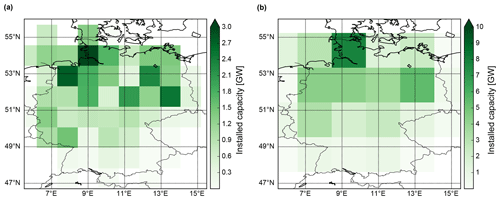
We derive nationally aggregated wind generation time series for the period 1901–2010 following the procedure detailed in Wohland et al. (2018). In short, the method consists of vertical extrapolation of 10 m wind speeds to 80 m hub height using a power law followed by the application of a standard turbine power curve at each grid point and finally a multiplication with the installed capacities (from OPSD, 2017). Projections of the installed capacities onto the grids of the 20th century reanalyses are shown in Fig. 1.
2.1 Twentieth century reanalyses
Wind speeds come from the full set of current 20th century reanalyses and are provided by two different centers: the European Centre for Medium-Range Weather Forecasts (ECMWF) and the National Oceanic and Atmospheric Administration (NOAA) from the USA. NOAA provided the first 20th century reanalysis named 20CR (Compo et al., 2011). 20CR is an atmospheric reanalysis that assimilates sea-level pressure observations only. In this study, we use the ensemble mean wind speeds from version 20CRv2c, which has 58 ensemble members. ECMWF followed a different approach and assimilates both sea-level pressure and marine wind observations. This difference in approaches yields substantial disagreement with respect to long-term wind speed trends (Wohland et al., 2019) but, as we show, there is large agreement regarding seasonal to multidecadal variability after subtraction of the linear trends. ECMWF provides an atmosphere (ERA20C; Poli et al., 2016) and a coupled atmosphere–ocean 20th century reanalysis (CERA20C; Laloyaux et al., 2018). ERA20C is deterministic (i.e., has only 1 member) and CERA20C comes with a 10-member ensemble. Unless otherwise stated, we report the CERA20C ensemble mean as the spread is usually very limited. Our analysis is based on 10 m wind speeds. In contrast to higher-altitude wind speeds, they are available for all 20th century reanalyses allowing us to apply the same methodology to all datasets and thereby ensuring comparability. We validate the approach in Sect. 3.
The longer temporal coverage comes at the cost of reduced spatial resolution as compared with modern reanalyses such as ERAINT (Dee et al., 2011), MERRA/MERRA2 (Rienecker et al., 2011) or ERA5 (Hennermann, 2018). ERA20C and CERA20C have a spatial resolution of and the 20CR resolution is even coarser (). While the datasets are thus clearly not well suited for site-specific assessments, they are sufficiently detailed for country-level assessments (see also Fig. 1). Temporal resolution is 3 h for all datasets and hence allows us to capture intraday effects.
2.2 Trend removal and timescale of interest
There is a demonstrated disagreement in the 20th century reanalyses in terms of wind speed trends, which originate from the assimilation of marine winds by ECMWF (Wohland et al., 2019). We thus remove the long-term (1901–2010) trends by subtraction of the zero-mean trend that is obtained via least-squares fitting of a linear fit function and subsequent subtraction of the trends mean:
where Graw(t) denotes the raw annual or seasonal time series, Gtrend(t) denotes the linear fit and 〈Gtrend(t)〉 is its mean value.
We focus on the long-term evolution of 20-year generation averages because 20 years is a typical lifetime for wind parks. Moreover, the averaging smooths the pronounced interannual variability, which has already been extensively studied elsewhere. Both energy system planning and wind park investment are forward procedures in the sense that infrastructure built today will be operated under the weather conditions of the future. We therefore decided to compute 20-year forward running means of wind power generation G20 as
where G(t′) denotes the annual wind power generation in year t′. To study the evolution in different seasons (winter DJF, spring MAM, summer JJA, autumn SON), we similarly compute the seasonal 20-year means as
where G(t′)season denotes the wind power generation in the respective season of year t′. Note that G20(t) and are ill defined at the end of the dataset when 20 years are not available. We thus only compute them up to 1990. We generally report normalized lifetime generation or normalized seasonal lifetime generation, which is obtained by division of G20(t) or with the 1901–2010 mean 〈G(t)〉 or 〈G(t)〉season, respectively.
2.2.1 Seasonality
In addition to seasonal generation averages, we report the seasonality S, which we define as the ratio of normalized winter to summer generation:
Seasonality is an important metric for power system design and has a large influence on optimum technology mixes (e.g., Heide et al., 2010). In Germany, wind power generation is generally higher in autumn and winter than in spring and summer. To ensure stable operation of the power system (i.e., a balance of generation and demand at all time steps), seasonality has to be accounted for in power system design. For example, the dimensioning of storage or backup infrastructure and optimum wind to solar mixes depend on the seasonality. For completeness, we provide an extended definition of seasonality , which also includes autumn and spring as
2.2.2 Bias
We use the term bias to assess whether the period covered by ERAINT is representative for the longer period covered by the 20th century reanalyses. For example, if the seasonality over 1979–2010 is higher than over 1900–2010, we call the seasonality estimates of modern reanalyses biased high.
2.3 Multitaper spectral estimation
We test significance of low-frequency components in the annual and seasonal wind generation time series using the multitaper method (MTM; Ghil, 2002). Classical approaches, such as Fourier spectral analysis, suffer from spectral leakage when applied to relatively short time series, hindering reliable assessments. MTM provides an alternative in that it calculates tapers that are designed to minimize leakage. We use K=3 tapers with a bandwidth of p=2 years as suggested by Ghil (2002) for a comparable time series. Eigentapers are weighted based on their eigenvalues and the computation is performed via the Python package spectrum (Cokelaer and Hasch, 2017).
Significance testing is based on the null hypothesis of red noise. The underlying process that creates a red-noise spectrum is referred to as a autoregressive model of first order or AR(1). The parameters of the red-noise spectrum, SR(f), are fitted to minimize the mismatch between the median smoothed real and the red-noise spectrum (as suggested by Ghil, 2002; Mann and Lees, 1996). A peak in the real spectrum S(f) at frequency f′ is considered significant at the 90 % level if
again following (Ghil, 2002). χ2(90 %,2 K) denotes the chi-squared distribution with 2 K degrees of freedom at a 90 % confidence level. White noise is a special case of red noise and is characterized by a constant spectrum (i.e., SW(f)=S0, where S0 is a real positive number). White noise is generated by an autoregressive model of zeroth order, AR(0).
2.4 Impacts on investments
In an investment decision, the installation and operational costs of an asset have to be compared with expected revenues. Taking into account risks and alternative investments, an investment is made if the expected revenues exceed the total costs by some amount. The expected revenue may be substantially flawed if it is based on only a couple of years of wind data. In contrast, decision makers that are aware of all modes of wind variability gain an advantage through more reliable revenue estimates.
To quantify this impact of low-frequency wind variability on wind park investments, we calculate the discounted lifetime cash inflows as
where γ=5.5 % yr−1 is the discount rate, Δη≈1.5 % yr−1 accounts for the decline in turbine performance (Staffell and Green, 2014), τ=20 years is the conservatively assumed lifetime, c is the revenue per generated unit of electricity and G is wind power generation. We set c to be constant because the German system is still designed to guarantee prices for wind park operators. Prior to the recent shift towards auctions, the price was determined politically. Since the latest reform of the renewable energy act in 2017, the price is determined via auctions but is still guaranteed over 20 years (BMWi, 2017). Both for old and new wind parks it is thus justified to use constant prices, albeit the price will differ depending on the date of construction and the auction outcome.
2.5 North Atlantic Oscillation
To gain more insight into the coevolution of wind generation variability and the general circulation of the atmosphere, we include the North Atlantic Oscillation (NAO). The NAO is the leading pattern of climate variability in the North Atlantic sector affecting weather and climate over Europe, particularly in winter (Marshall et al., 2001). It is here defined as the first principle component of sea-level pressure over the area 20–80∘ N and 90∘ W–40∘ E as detailed in Omrani et al. (2016). Our NAO index is computed from sea-level pressure data from the Hadley Center (Rayner, 2003) over the winter months December, January and February.
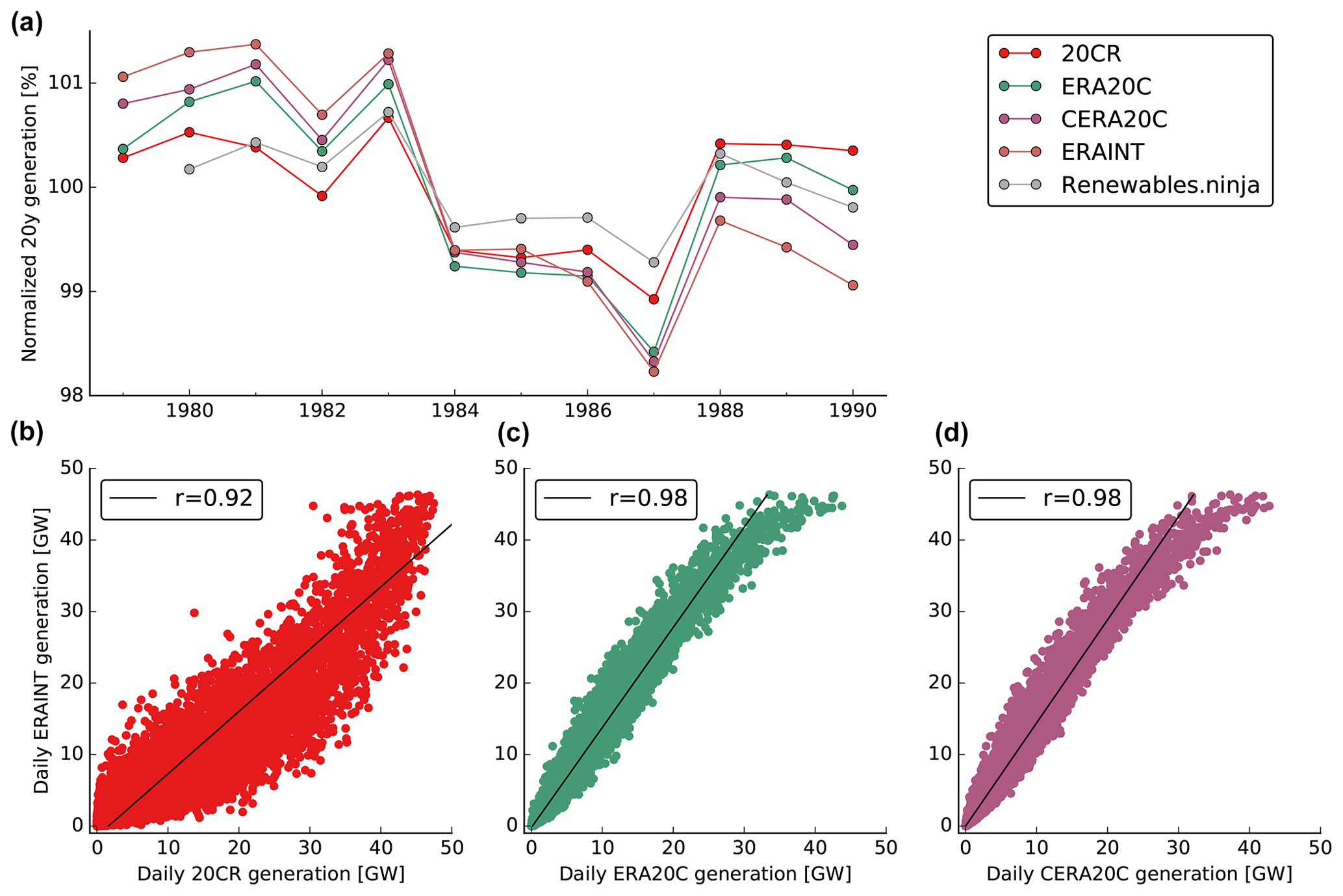
Figure 2German wind power generation from modern reanalyses (ERAINT, MERRA2) and 20th century reanalyses (20CR, ERA20C, CERA20C) for period of overlap. (a) Normalized lifetime generation (i.e., the reported value for 1990 is the average wind power generation of the years 1990–2009 normalized with the long-term mean). “Renewables.ninja” is an openly available generation dataset that is based on MERRA2. (b–d) Scatter plots of daily generation from ERAINT versus daily values from 20CR (b), ERA20C (c) and CERA20C (d) for the 30-year period from 1979 to 2009. The Pearson correlation coefficient, r, between the daily data is given in the legends. The data are shown prior to long-term trend removal, which was performed for the centennial analysis (see Sect. 2).
In a recent study, we have shown that ERAINT has skill to reproduce reported wind power generation in Germany (Wohland et al., 2018). It thus appears logical to test the 20th century reanalyses by comparison with ERAINT over the overlapping period (1979–2009). We also add the widely used Renewables.ninja wind energy dataset that is based on MERRA2 (Staffell and Pfenninger, 2016).
The evolution of the normalized lifetime mean generation is similar for all reanalyses under consideration (see Fig. 2a). All start with a period of high values that is followed by roughly 5 years of low values. Towards the end, the normalized lifetime generation recovers but not to the same levels as in the first couple of years.
On a finer temporal scale, there are good correlations between the daily generations based on ERAINT and 20CR and ERA20C and CERA20C (see Fig. 2b–d). 20CR overestimates daily generation (slope <1 in Fig. 2b). In contrast, ERA20C and CERA20C underestimate daily generation (slopes >1 in Fig. 2c, d). This systematic over- or underestimation of daily wind generations, however, is of minor importance in this study because it is reduced by normalization with the long-term mean. All 20th century reanalyses agree well with ERAINT for very high daily generations larger than around 40 GW. Pearson correlation is high for 20CR (r=0.92) and even higher for the ECMWF products (r=0.98). A similar result is found for the RMSE, which is 4.3 GW for 20CR and around 1.3 GW for ERA20C and CERA20C, again indicating larger agreement across the ECMWF reanalyses. This larger agreement could be due to more similar spatial resolutions that allow us to capture the same processes in (C)ERA20C as in ERAINT. It may also reflect the common institutional origin as ERAINT and (C)ERA20C have been developed at ECMWF and are based on different versions of the same model. In any case, the substantial agreement in the detrended time series on different timescales creates confidence in the 20th century reanalyses.
From visual inspection, there also seems to be a downward trend over the period 1979–1990. A trend analysis of the ERAINT data indeed reveals a significant (at the 99 % level) downward trend of the normalized lifetime generation, highlighting the relevance of long-term assessments. However, this trend should be interpreted cautiously as it is calculated using only 11 (not independent) values of G20. The remainder of the paper is therefore based on longer time series to allow more robust assessments of multidecadal variability.
4.1 Trends
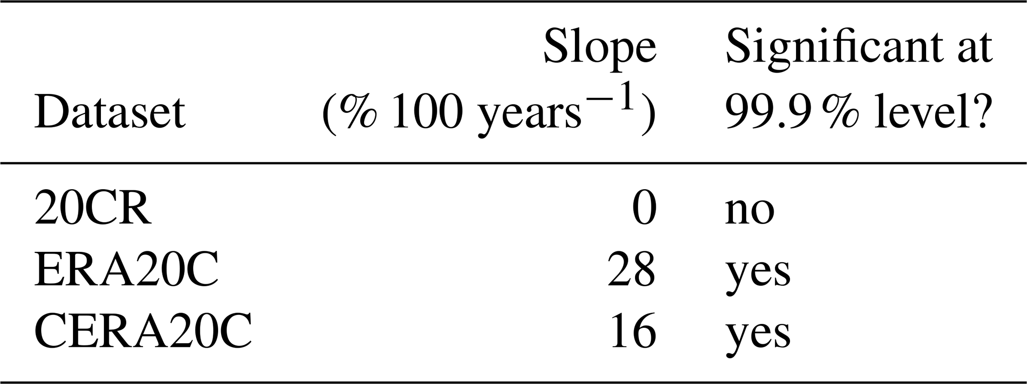
We find ERA20C and CERA20C to feature statistically highly significant trends (see Table 1). In both datasets, the trends are strong: ERA20C reports 28 % higher wind power generation at the end of the 20th century as compared to its beginning. The corresponding increase in CERA20C is substantial (16 % increase in a hundred years) but roughly half as large. In contrast, there is no significant trend in 20CR.
The existence of these trends comes as no surprise given strong long-term trends in (C)ERA20C surface wind speeds over large parts of the world (Wohland et al., 2019). In our previous publication, we showed that the trends originate from the assimilated marine wind speeds that also feature very strong long-term trends. They are likely spurious and caused by the evolving measurement technique. In addition to wind speed trends, ERA20C also features trends in marine sea-level pressure gradients that are not in line with observations (Bloomfield et al., 2018). All following analyses are therefore based on detrended time series.
Table 1Trend characteristics are shown. Slopes are rounded to integer values and the CERA20C slope corresponds to the mean of the slopes of the individual ensemble members. Significance is tested against the null hypothesis of no trend and using a two-sided t test. For CERA20C, all streams feature significant trends individually.
4.2 Low-frequency variability in normalized lifetime wind generation
After subtraction of the trends, there is large agreement among the datasets regarding multidecadal variability in normalized lifetime generation (see Fig. 3). Maxima and minima of annual and seasonal time series coincide for ERA20C, CERA20C and 20CR. The amplitude of variability is also comparable among the datasets for all seasons and the annual values. Only in September–October–November (SON) is there disagreement from 1960 onwards as 20CR reports values that are 5 % to 10 % off the (C)ERA20C values. Generally, there is stronger variability in seasonal compared to annual generation, hinting at compensating effects between seasons. In June–July–August (JJA), for example, the maximum to minimum difference is around 15 %. This compares to 5 % to 10 % maximum to minimum difference for the annual values.
German annual generation is dominated by winter generation due to generally stronger winds in winter. This winter dependence explains the high similarity between the annual and wintertime series (compare Fig. 3a with c) and also the high correlation of r=0.71 between them (see Fig. 3b). On the timescales considered here, there is also a weak anticorrelation between the annual and the summer values () and between the summer and autumn values ().
The ratio of winter to summer generation (i.e., seasonality) is characterized by strong multidecadal variability. While the maximum 20-year seasonality is between 110 % and almost 120 % (dependent on the dataset), the minimum lies between 80 % and 90 % (see Fig. 3g). If an extended definition of seasonality is applied, the amplitude of the variability is reduced, but the maximum to minimum difference still ranges around 15 % to 20 % (see Fig. 3h).
In winter there is also a good connection between 20-year mean anomalies of the North Atlantic Oscillation (NAO) and normalized lifetime generation as highlighted by correlation coefficients between them that range from r=0.7 to r=0.76 for the different datasets (see Fig. 4a). This relation is consistent with the NAO being the dominant pattern of wintertime climate variability in the North Atlantic sector (Marshall et al., 2001). The agreement is strongest on multidecadal timescales and it is particularly high since 1960. However, a peak in normalized lifetime wind generation around mid-century is not paralleled by a similar feature in the NAO.
Modern reanalyses, such as ERAINT, are too short to capture these modes of low-frequency variability (see blue arrows in Fig. 3). Unfortunately, ERAINT not only fails to capture these effects but also provides biased high estimates in some cases. For example, the seasonality reported by ERAINT, coincides with above-average values of seasonality and is hence not representative in general (see Fig. 3g). The same is true for annual and winter generation. Moreover, ERAINT begins at a time of maximum normalized lifetime wind generation. ERAINT-based trend assessments can thus misidentify the downward part of reoccurring cycles as trends (as discussed in Sect. 3). Similarly, the decline of autumn generation since the 1970s could be falsely interpreted as a trend.
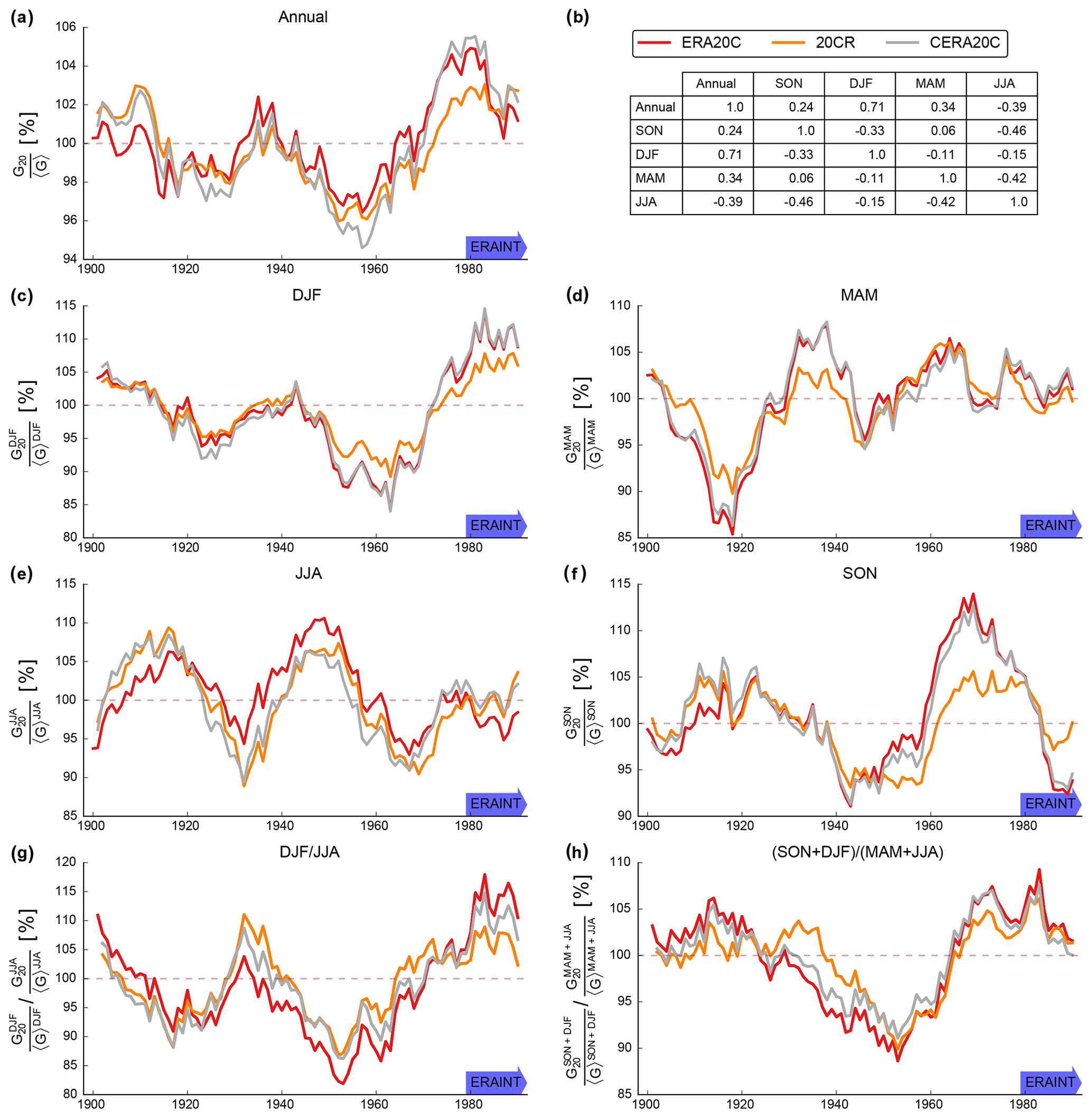
Figure 3Normalized lifetime generation from German wind parks. Time series are based on detrended 20th century reanalyses. The panels show annual (a) and seasonal (c–f) time series. Different versions of the seasonality are also displayed (g–h) and correlations between seasons are reported for ERA20C (b). The data have been smoothed by application of a running mean 20-year forward filter (i.e., the reported value for 1900 is the average of the years 1900–1919). The blue arrow highlights the limited coverage of ERAINT.
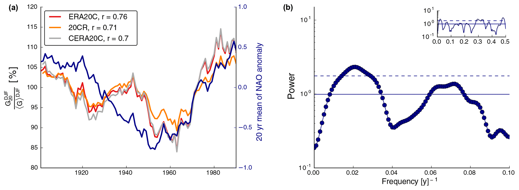
Figure 4Relation between normalized lifetime winter generation and the winter North Atlantic Oscillation. Time series of wind power generation (in red, orange and gray) refer to the left y axis while the NAO time series (in blue) refers to the right y axis (a). Pearson correlation coefficients, r, are calculated between the 20-year mean NAO anomaly and the 20-year mean DJF wind power generation. MTM spectrum of the winter NAO (bullets in b), focusing on the low-frequency interval of the spectrum. Solid lines represent the fitted spectrum of an AR(1) process that is used for significance testing and the dashed lines correspond to the 90 % confidence level (see Sect. 2 for details).
4.3 Spectral analysis
We perform multitaper spectral analysis for detrended annual and seasonal German wind power generation over the period 1901–2010 (Fig. 5). No prior smoothing or filtering is applied. A focus is given to the low-frequency part of the spectrum with frequencies of less than 0.1 yr−1, which corresponds to at least 10-year periods. There are statistically significant low-frequency peaks in all seasons with different levels of agreement among reanalyses. All reanalyses feature a significant peak in MAM (f≈0.04 yr−1 or yr) and JJA (f≈0.03 yr−1 or yr), and the latter is also clearly visible in the time series (see Fig. 3e). In SON, CERA20C and ERA20C report a clearly significant peak that is also almost significant in 20CR (f≈0.02 yr−1 or yr). In winter there is a spectral peak with a period of around 50 years (f≈0.02 yr−1) that is related to the NAO (see Fig. 4b). This connection to a physical pattern of climate variability suggests that the peak is not a statistical artifact, despite its low statistical significance. The generally high agreement among the reanalyses adds confidence to the existence of multidecadal periodicities during the historical period.
Spectral peaks generally do not exist at the same frequencies in different seasons. This implies that the relevant processes vary by season. While the winter NAO explains a large share of the winter variability, similar explanations can currently not be given for the other seasons.
Interestingly, the AR(1) fit to the median-smoothed spectra does not reveal red noise but white noise (except for MAM), in agreement with the understanding of atmospheric variability as a process that is white to first order (Wunsch, 1999). This can be seen by the thin solid lines in Fig. 5, which display the fitted AR(1) spectra: they are virtually flat, i.e., virtually independent of the frequency. For example, in JJA (Fig. 5d), the power of the AR(1) fit is 100 (GWh/GWh)2 for all frequencies. White noise implies that the system does not have relevant memory from one year to the next but rather behaves erratically on year-to-year timescales.
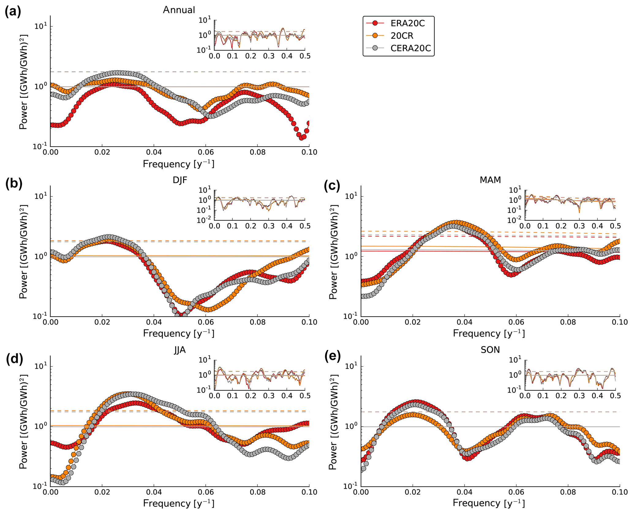
Figure 5Spectral analysis of the wind generation time series using the multitaper method (MTM). Panels report annual (a) and seasonal spectra (b–e). Focus is given to the low-frequency component with frequencies of less than 0.1 yr−1 while the full spectrum is shown in the inset of each panel. Solid lines represent the fitted spectrum of an AR(1) process that is used for significance testing and the dashed lines correspond to the 90 % confidence level for each dataset (see Sect. 2 for details).

Figure 6Long-term evolution of normalized discounted lifetime cash inflows of a wind park whose generation follows the German mean. A lifetime of 20 years, aging of 1.5 % yr−1 and a discount rate of 5.5 % yr−1 are assumed. The time series ends in 1990 because the underlying reanalyses end in 2010.
4.4 Relevance for investment decisions
In addition to the relevance of low-frequency variability for system design, the long lifetime of wind parks makes returns on individual investment susceptible to low-frequency variability, and not taking this susceptibility into account has substantial economic implications. The effect is illustrated in Fig. 6 where the discounted lifetime cash inflow of a wind park that follows the German mean wind generation is shown. The values are normalized such that 100 % refers to the 1901–2010 mean. This graph shows variability in a wind park's cash inflow between a maximum of 104 % to 107 % and a minimum of 95 % to 97 % dependent on the phase of low-frequency climate variability at the commissioning date. In other words, a wind park created in 1955 would produce 7 %–12 % less revenue than one created in 1975. Recall that we abstract from technology innovations throughout the entire article. Dependent on the individual project characteristics, most notably the ratio of the investment to the expected lifetime cash inflows, a few per cent more or less on the income side can turn an average project into a very profitable one or might leave a slightly profitable project unprofitable. Roughly between 1960 and 1975, there was a linear increase in cash inflows, which has been followed by a decrease since 1980. Assessments based on ERAINT may tend to overestimate discounted lifetime cash inflows as ERAINT coincides with a period of high wind generation.
Based on the full set of current 20th century reanalyses (20CR, ERA20C, CERA20C), we have shown that multidecadal variability matters for wind energy in Germany. There are statistically significant modes of generation variability on timescales of 25 to 50 years in spring, summer and autumn. In winter, there is a spectral peak with a period of around 50 years that is related to the NAO. This connection to a physical pattern of climate variability suggests that the peak is not a statistical artifact, despite its low statistical significance. Wind power generation reached a multidecadal maximum around 1980 implying that trend assessments starting in 1980 suffer from a sampling bias. The downward sloping fraction of multidecadal variability should not be confused with a long-term trend and an extrapolation of the trend into the future is misleading. These results are relevant in contextualizing suggestions that wind speeds are globally decreasing (Vautard et al., 2010).
Our results imply that in addition to relatively intuitive timescales (diurnal, seasonal, annual) slower and less intuitive modes of variability ought to be included in energy assessments too. While current modern reanalyses are too short to capture multidecadal wind generation variability, future products may be better suited due to extended temporal coverage (e.g., ERA5 will start in 1950 and is expected to be entirely published in late 2019).
One of the most relevant results for power system design is the variability in seasonality (defined as the ratio of winter to summer generation here). Far from being constant, 20-year mean seasonality varies by almost ±15 %. As the seasonal evolution of generation is one main factor to determine optimum contributions of wind and photovoltaics (Heide et al., 2010), such optimum shares should also be considered time series that vary on timescales of 50 years or so. This variability calls for an ongoing and dynamic redesign of power systems to follow climate variability. Even though the lifetime of individual power system components (e.g., transmission lines or power plants) is very long, additions, replacements and retirements occur frequently within the entire power system. These events theoretically allow for adaptive reactions to multidecadal variability. ERAINT samples a seasonality maximum and therefore reports biased high seasonality. This bias implies that lifetime wind power generation is most often more stable throughout the year than would be expected from ERAINT, facilitating system integration. In the bigger picture, it may be relevant to rethink whether changes in seasonality that were attributed to climate change in earlier studies (e.g., Reyers et al., 2016) may simply reflect natural variability.
There are also implications for individual wind park projects as their profitability is strongly influenced by climate variability on long timescales. The same wind park commissioned in different phases of low-frequency generation variability can have discounted lifetime cash inflows anywhere between 95 % and 107 % of the mean value with potentially severe impacts on profitability. To give an impression of scale, as the current German wind park fleet represents a EUR 95 billion investment, this translates into a lifetime revenue spread on the order of EUR 10 billion in Germany alone.
Our study raises new questions. While Germany was chosen as an exemplary case due to its current high deployment of wind turbines, other, and larger, areas should also be studied. Are there compensating effects across Europe? If yes, expansion of the transmission network and optimized siting could help mitigate multidecadal variability in the same fashion that it helps to smooth synoptic generation variability (e.g., Rodriguez et al., 2014; Grams et al., 2017; Santos-Alamillos et al., 2017). This study is restricted to wind energy because we doubt the reanalysis skill to capture cloud dynamics sufficiently well. Nevertheless, it would be of high interest to investigate low-frequency variability in other types of renewable generation: do similar modes exist for photovoltaics and hydropower? In addition to the winter link between wind power generation and the NAO, other connections between multidecadal renewable generation and large-scale patterns of climate variability might exist. They could contribute to a process-based understanding and should therefore be investigated in future work. Lastly, climate models are, in theory, an excellent tool to quantify and study natural climate variability as time series of arbitrary length can be obtained. Multidecadal variability can thus be sampled substantially better compared to 20th century reanalyses. However, it remains to be shown whether climate models are capable to reproduce multidecadal variability that is relevant for the energy sector.
This paper relies on wind speeds from different 20th century reanalysis that are openly available through ECMWF (http://apps.ecmwf.int/datasets/data/era20c-daily/levtype=sfc/type=an/, last access: 9 September 2019) and NOAA (https://www.esrl.noaa.gov/psd/data/gridded/data.20thC_ReanV2c.monolevel.html, last access: 9 September 2019). We also use the end of 2016 wind fleet configuration as reported by the Open Power System Data, which is also openly available online (https://data.open-power-system-data.org/renewable_power_plants/, last access: 9 September 2019). The programming is done in Python and the code is shared upon reasonable request to the authors.
JW initiated the collaboration, developed the methodology, analyzed the data, produced all figures and wrote most of the article. DW contributed to the methodology and interpretation of the data and supervised the research. NEO and NK contributed to the development of the methodology and the interpretation of the results. All authors contributed ideas, gave feedback and helped to improve the article.
The authors declare that they have no conflict of interest.
We thank ECMWF for making ERA20C and CERA20C publicly available. We thank NOAA for making 20CRv2c available. Jan Wohland thanks the HITEC graduate school at Forschungszentrum Jülich for a travel grant.
This research has been supported by the Helmholtz Association (grant nos. VH-NG-1025 and Energiesystem 2050).
The article processing charges for this open-access
publication were covered by a Research
Centre of the Helmholtz Association.
This paper was edited by Julie Lundquist and reviewed by Sonia Jerez and one anonymous referee.
Ba, J., Keenlyside, N. S., Latif, M., Park, W., Ding, H., Lohmann, K., Mignot, J., Menary, M., Otterå, O. H., Wouters, B., Salas y Melia, D., Oka, A., Bellucci, A., and Volodin, E.: A multi-model comparison of Atlantic multidecadal variability, Clim. Dynam., 43, 2333–2348, https://doi.org/10.1007/s00382-014-2056-1, 2014. a
Bett, P. E., Thornton, H. E., and Clark, R. T.: European wind variability over 140 yr, Adv. Sci. Res., 10, 51–58, https://doi.org/10.5194/asr-10-51-2013, 2013. a
Bett, P. E., Thornton, H. E., and Clark, R. T.: Using the Twentieth Century Reanalysis to assess climate variability for the European wind industry, Theor. Appl. Climatol., 127, 61–80, https://doi.org/10.1007/s00704-015-1591-y, 2017. a
Bloomfield, H., Shaffrey, L., Hodges, K. I., and Vidale, P. L.: A critical assessment of the long term changes in the wintertime surface Arctic Oscillation and Northern Hemisphere storminess in the ERA20C reanalysis, Environ. Res. Lett., https://doi.org/10.1088/1748-9326/aad5c5, 2018. a
BMWi: Fragen und Antworten zum EEG 2017, Bundesministerium für Wirtschaft und Energie, p. 9, 2017. a
BMWi: Zeitreihen zur Entwicklung der erneuerbaren Energien in Deutschland, Bundesministerium für Wirtschaft und Energie, p. 46, 2018. a
Brayshaw, D. J., Troccoli, A., Fordham, R., and Methven, J.: The impact of large scale atmospheric circulation patterns on wind power generation and its potential predictability: A case study over the UK, Renew. Energ., 36, 2087–2096, https://doi.org/10.1016/j.renene.2011.01.025, 2011. a
Cokelaer, T. and Hasch, J.: 'Spectrum': Spectral Analysis in Python, Journal of Open Source Software, 2, 348, https://doi.org/10.21105/joss.00348, 2017. a
Compo, G. P., Whitaker, J. S., Sardeshmukh, P. D., Matsui, N., Allan, R. J., Yin, X., Gleason, B. E., Vose, R. S., Rutledge, G., Bessemoulin, P., Brönnimann, S., Brunet, M., Crouthamel, R. I., Grant, A. N., Groisman, P. Y., Jones, P. D., Kruk, M. C., Kruger, A. C., Marshall, G. J., Maugeri, M., Mok, H. Y., Nordli, O., Ross, T. F., Trigo, R. M., Wang, X. L., Woodruff, S. D., and Worley, S. J.: The Twentieth Century Reanalysis Project, Q. J. Roy. Meteor. Soc., 137, 1–28, https://doi.org/10.1002/qj.776, 2011. a
Dee, D. P., Uppala, S. M., Simmons, A. J., Berrisford, P., Poli, P., Kobayashi, S., Andrae, U., Balmaseda, M. A., Balsamo, G., Bauer, P., Bechtold, P., Beljaars, A. C. M., van de Berg, L., Bidlot, J., Bormann, N., Delsol, C., Dragani, R., Fuentes, M., Geer, A. J., Haimberger, L., Healy, S. B., Hersbach, H., Hólm, E. V., Isaksen, L., Kållberg, P., Köhler, M., Matricardi, M., McNally, A. P., Monge-Sanz, B. M., Morcrette, J.-J., Park, B.-K., Peubey, C., de Rosnay, P., Tavolato, C., Thépaut, J.-N., and Vitart, F.: The ERA-Interim reanalysis: configuration and performance of the data assimilation system, Q. J. Roy. Meteor. Soc., 137, 553–597, https://doi.org/10.1002/qj.828, 2011. a
Ely, C. R., Brayshaw, D. J., Methven, J., Cox, J., and Pearce, O.: Implications of the North Atlantic Oscillation for a UK-Norway Renewable power system, Energ. Policy, 62, 1420–1427, https://doi.org/10.1016/j.enpol.2013.06.037, 2013. a
Ghil, M.: Advanced spectral methods for climatic time series, Rev. Geophys., 40, 1003, https://doi.org/10.1029/2000RG000092, 2002. a, b, c, d
Gonzalez Aparcio, I., Zucker, A., Careri, F., Monforti, F., Huld, T., and Badger, J.: EMHIRES dataset; Part 1: Wind power generation, Tech. Rep. EUR 28171 EN, Joint Research Center, 2016. a
Grams, C. M., Beerli, R., Pfenninger, S., Staffell, I., and Wernli, H.: Balancing Europe’s wind-power output through spatial deployment informed by weather regimes, Nat. Clim. Change, 7, 557–562, https://doi.org/10.1038/nclimate3338, 2017. a
Heide, D., von Bremen, L., Greiner, M., Hoffmann, C., Speckmann, M., and Bofinger, S.: Seasonal optimal mix of wind and solar power in a future, highly renewable Europe, Renew. Energ., 35, 2483–2489, https://doi.org/10.1016/j.renene.2010.03.012, 2010. a, b
Heide, D., Greiner, M., Von Bremen, L., and Hoffmann, C.: Reduced storage and balancing needs in a fully renewable European power system with excess wind and solar power generation, Renew. Energ., 36, 2515–2523, 2011. a
Hennermann, K.: ERA5 data documentation, available at: https://confluence.ecmwf.int//display/CKB/ERA5+data+documentation (last access: 9 September 2019), 2018. a
IEA/IRENA: Perspectives for the Energy Transition, International Energy Agency/International Renewable Energy Agency, Tech. rep., 2017. a
Jerez, S., Trigo, R. M., Vicente-Serrano, S. M., Pozo-Vázquez, D., Lorente-Plazas, R., Lorenzo-Lacruz, J., Santos-Alamillos, F., and Montávez, J. P.: The Impact of the North Atlantic Oscillation on Renewable Energy Resources in Southwestern Europe, J. Appl. Meteorol. Climatol., 52, 2204–2225, https://doi.org/10.1175/JAMC-D-12-0257.1, 2013. a
Jerez, S., Tobin, I., Turco, M., Jiménez-Guerrero, P., Vautard, R., and Montávez, J. P.: Future changes, or lack thereof, in the temporal variability of the combined wind-plus-solar power production in Europe, Renew. Energ., 139, 251–260, 2019. a
Karnauskas, K. B., Lundquist, J. K., and Zhang, L.: Southward shift of the global wind energy resource under high carbon dioxide emissions, Nat. Geosci., 11, 38–43, https://doi.org/10.1038/s41561-017-0029-9, 2018. a
Laloyaux, P., de Boisseson, E., Balmaseda, M., Bidlot, J.-R., Broennimann, S., Buizza, R., Dalhgren, P., Dee, D., Haimberger, L., Hersbach, H., Kosaka, Y., Martin, M., Poli, P., Rayner, N., Rustemeier, E., and Schepers, D.: CERA-20C: A coupled reanalysis of the Twentieth Century, J. Adv. Model. Earth Syst., 10, 1172–1195, https://doi.org/10.1029/2018MS001273, 2018. a
Mann, M. E. and Lees, J. M.: Robust estimation of background noise and signal detection in climatic time series, Clim. Change, 33, 409–445, https://doi.org/10.1007/BF00142586, 1996. a
Marshall, J., Kushnir, Y., Battisti, D., Chang, P., Czaja, A., Dickson, R., Hurrell, J., McCartney, M., Saravanan, R., and Visbeck, M.: North Atlantic climate variability: phenomena, impacts and mechanisms, Int. J. Climatol., 21, 1863–1898, https://doi.org/10.1002/joc.693, 2001. a, b
Moraes, L., Bussar, C., Stoecker, P., Jacqué, K., Chang, M., and Sauer, D.: Comparison of long-term wind and photovoltaic power capacity factor datasets with open-license, Appl. Energ., 225, 209–220, https://doi.org/10.1016/j.apenergy.2018.04.109, 2018. a
Omrani, N.-E., Bader, J., Keenlyside, N. S., and Manzini, E.: Troposphere–stratosphere response to large-scale North Atlantic Ocean variability in an atmosphere/ocean coupled model, Clim. Dynam., 46, 1397–1415, https://doi.org/10.1007/s00382-015-2654-6, 2016. a, b
OPSD: Renewable power plants (version 16/02/17),, available at: https://data.open-power-system-data.org/renewable_power_plants/ (last access: 9 September 2019), 2017. a, b
Poli, P., Hersbach, H., Dee, D. P., Berrisford, P., Simmons, A. J., Vitart, F., Laloyaux, P., Tan, D. G. H., Peubey, C., Thépaut, J.-N., Trémolet, Y., Hólm, E. V., Bonavita, M., Isaksen, L., and Fisher, M.: ERA-20C: An Atmospheric Reanalysis of the Twentieth Century, J. Climate, 29, 4083–4097, https://doi.org/10.1175/JCLI-D-15-0556.1, 2016. a
Pryor, S. and Barthelmie, R.: Climate change impacts on wind energy: A review, Renew. Sustain. Energ. Rev., 14, 430–437, https://doi.org/10.1016/j.rser.2009.07.028, 2010. a
PWC: Europas Top 100, available at: https://www.pwc.de/de/kapitalmarktorientierte-unternehmen/pwc-infografik-europas-top-100-unternehmen.pdf (last access: 9 September 2019), 2018. a
Rayner, N. A.: Global analyses of sea surface temperature, sea ice, and night marine air temperature since the late nineteenth century, J. Geophys. Res., 108, 4407, https://doi.org/10.1029/2002JD002670, 2003. a
Reyers, M., Moemken, J., and Pinto, J. G.: Future changes of wind energy potentials over Europe in a large CMIP5 multi-model ensemble, Int. J. Climatol., 36, 783–796, https://doi.org/10.1002/joc.4382, 2016. a, b
Rienecker, M. M., Suarez, M. J., Gelaro, R., Todling, R., Bacmeister, J., Liu, E., Bosilovich, M. G., Schubert, S. D., Takacs, L., Kim, G.-K., Bloom, S., Chen, J., Collins, D., Conaty, A., da Silva, A., Gu, W., Joiner, J., Koster, R. D., Lucchesi, R., Molod, A., Owens, T., Pawson, S., Pegion, P., Redder, C. R., Reichle, R., Robertson, F. R., Ruddick, A. G., Sienkiewicz, M., and Woollen, J.: MERRA: NASA’s Modern-Era Retrospective Analysis for Research and Applications, J. Climate, 24, 3624–3648, https://doi.org/10.1175/JCLI-D-11-00015.1, 2011. a
Ringkjøb, H.-K., Haugan, P. M., and Solbrekke, I. M.: A review of modelling tools for energy and electricity systems with large shares of variable renewables, Renew. Sustain. Energ. Rev., 96, 440–459, https://doi.org/10.1016/j.rser.2018.08.002, 2018. a
Rodriguez, R. A., Becker, S., Andresen, G. B., Heide, D., and Greiner, M.: Transmission needs across a fully renewable European power system, Renew. Energ., 63, 467–476, https://doi.org/10.1016/j.renene.2013.10.005, 2014. a
Rogelj, J., Luderer, G., Pietzcker, R. C., Kriegler, E., Schaeffer, M., Krey, V., and Riahi, K.: Energy system transformations for limiting end-of-century warming to below 1.5 ∘C, Nat. Clim. Change, 5, 519–527, https://doi.org/10.1038/nclimate2572, 2015. a
Santos-Alamillos, F. J., Brayshaw, D. J., Methven, J., Thomaidis, N. S., Ruiz-Arias, J. A., and Pozo-Vázquez, D.: Exploring the meteorological potential for planning a high performance European electricity super-grid: optimal power capacity distribution among countries, Environ. Res. Lett., 12, 114030, https://doi.org/10.1088/1748-9326/aa8f18, 2017. a
Schlachtberger, D., Brown, T., Schramm, S., and Greiner, M.: The benefits of cooperation in a highly renewable European electricity network, Energy, 134, 469–481, https://doi.org/10.1016/j.energy.2017.06.004, 2017. a
Schleussner, C.-F., Rogelj, J., Schaeffer, M., Lissner, T., Licker, R., Fischer, E. M., Knutti, R., Levermann, A., Frieler, K., and Hare, W.: Science and policy characteristics of the Paris Agreement temperature goal, Nat. Clim. Change, 6, 827–835, https://doi.org/10.1038/nclimate3096, 2016. a
Schlott, M., Kies, A., Brown, T., Schramm, S., and Greiner, M.: The impact of climate change on a cost-optimal highly renewable European electricity network, Appl. Energ., 230, 1645–1659, https://doi.org/10.1016/j.apenergy.2018.09.084, 2018. a
Staffell, I. and Green, R.: How does wind farm performance decline with age?, Renew. Energ., 66, 775–786, https://doi.org/10.1016/j.renene.2013.10.041, 2014. a
Staffell, I. and Pfenninger, S.: Using bias-corrected reanalysis to simulate current and future wind power output, Energy, 114, 1224–1239, https://doi.org/10.1016/j.energy.2016.08.068, 2016. a, b
Tobin, I., Jerez, S., Vautard, R., Thais, F., van Meijgaard, E., Prein, A., Deque, M., Kotlarski, S., Maule, C. F., Nikulin, G., Noel, T., and Teichmann, C.: Climate change impacts on the power generation potential of a European mid-century wind farms scenario, Environ. Res. Lett., 11, 034013, https://doi.org/10.1088/1748-9326/11/3/034013, 2016. a
Vautard, R., Cattiaux, J., Yiou, P., Thépaut, J.-N., and Ciais, P.: Northern Hemisphere atmospheric stilling partly attributed to an increase in surface roughness, Nat. Geosci., 3, 756–761, https://doi.org/10.1038/ngeo979, 2010. a, b
Weber, J., Wohland, J., Reyers, M., Moemken, J., Hoppe, C., Pinto, J. G., and Witthaut, D.: Impact of climate change on backup energy and storage needs in wind-dominated power systems in Europe, PLOS ONE, 13, e0201457, https://doi.org/10.1371/journal.pone.0201457, 2018. a
Wohland, J., Reyers, M., Weber, J., and Witthaut, D.: More homogeneous wind conditions under strong climate change decrease the potential for inter-state balancing of electricity in Europe, Earth Syst. Dynam., 8, 1047–1060, https://doi.org/10.5194/esd-8-1047-2017, 2017. a
Wohland, J., Reyers, M., Märker, C., and Witthaut, D.: Natural wind variability triggered drop in German redispatch volume and costs from 2015 to 2016, PLOS ONE, 13, e0190707, https://doi.org/10.1371/journal.pone.0190707, 2018. a, b
Wohland, J., Omrani, N.-E., Witthaut, D., and Keenlyside, N. S.: Inconsistent Wind Speed Trends in Current Twentieth Century Reanalyses, J. Geophys. Res.-Atmos., 124, 1931–1940, https://doi.org/10.1029/2018JD030083, 2019. a, b, c
Wunsch, C.: The Interpretation of Short Climate Records, with Comments on the North Atlantic and Southern Oscillations, B. Am. Meteorol. Soc., 80, 245–255, https://doi.org/10.1175/1520-0477(1999)080<0245:TIOSCR>2.0.CO;2, 1999. a
Ziegler, L., Gonzalez, E., Rubert, T., Smolka, U., and Melero, J. J.: Lifetime extension of onshore wind turbines: A review covering Germany, Spain, Denmark, and the UK, Renew. Sustain. Energ. Rev., 82, 1261–1271, https://doi.org/10.1016/j.rser.2017.09.100, 2018. a