Improving mesoscale wind speed forecasts using lidar-based observation nudging for airborne wind energy systems

Airborne wind energy systems (AWESs) aim to operate at altitudes above conventional wind turbines where reliable high-resolution wind data are scarce. Wind light detection and ranging (lidar) measurements and mesoscale models both have their advantages and disadvantages when assessing the wind resource at such heights. This study investigates whether assimilating measurements into the mesoscale Weather Research and Forecasting (WRF) model using observation nudging generates a more accurate, complete data set. The impact of continuous observation nudging at multiple altitudes on simulated wind conditions is compared to an unnudged reference run and to the lidar measurements themselves. We compare the impact on wind speed and direction for individual days, average diurnal variability and long-term statistics. Finally, wind speed data are used to estimate the optimal traction power and operating altitudes of AWES. Observation nudging improves the WRF accuracy at the measurement location. Close to the surface the impact of nudging is limited as effects of the air–surface interaction dominate but becomes more prominent at mid-altitudes and decreases towards high altitudes. The wind speed frequency distribution shows a multi-modality caused by changing atmospheric stability conditions. Therefore, wind speed profiles are categorized into various stability conditions. Based on a simplified AWES model, the most probable optimal altitude is between 200 and 600 m. This wide range of heights emphasizes the benefit of such systems to dynamically adjust their operating altitude.

1 Introduction

The prospects of higher energy potential, more consistent strong winds and less turbulence in comparison to near-surface winds has sparked interest in mid-altitude wind energy systems, with “mid-altitude” defined here as heights above 100 m and below 1500 m,. Airborne wind energy systems are a novel class of renewable energy technology that harvest stronger winds at altitudes which are unreachable by current wind turbines, at potentially significantly reduced capital cost (Lunney et al., 2017; Fagiano and Milanese, 2012). For practical and economical reasons we focus on resource assessment within the lower part of the atmosphere, an altitude range spanned by the highly variable boundary layer. Unlike conventional wind energy, which has converged to a single concept with three blades and a conical tower, several different AWES designs are under investigation by numerous companies and research institutes worldwide (Cherubini et al., 2015). Various concepts are competing for entry into the market, ranging from ring-shaped aerostats to rigid wings and soft kites with different sizes, rated power and altitude ranges. Since this technology is still in an early stage, none are currently commercially available.

Developers and operators of large conventional wind turbines, AWES and drones require accurate wind data to estimate power output and mechanical loads. They currently rely on oversimplified approximations such as the logarithmic wind profile (Optis et al., 2016) or coarsely resolved reanalysis data sets (Archer and Caldeira, 2009; Bechtle et al., 2019) as the applicability of conventional spectral wind models (Burton, 2011) has not been verified for these altitudes. The first investigations (Fechner and Schmehl, 2018) resorting to the Mann model (Mann, 1994; IEC, 2005) have been conducted.

Recent advancements in wind lidar technology enable measurements at higher altitudes. This measurement technique, however, suffers from reduced data availability with increasing altitude caused by a decrease in aerosol density, which is needed for the backscattering of the lidar signal (Peña et al., 2015). No mid-altitude measurement device can reliably gather long-term, high-frequency data. The temporal and spatial resolution of lidar devices is insufficient to precisely measure high-frequency fluctuations, but estimated turbulence intensity correlates with sonic turbulence measurements for lower altitudes (Sathe et al., 2011). Balloon-mounted sonic anemometers are in early development (Canut et al., 2016). The expensive and time-consuming nature of measurements motivates the usage of numerical weather prediction models, such as the mesoscale Weather Research and Forecasting (WRF) model, as adequate tools to assess the synoptic characteristics of the atmospheric boundary layer (ABL) (Al-Yahyai et al., 2010). These models typically have a spatial resolution that ranges from 1 km to tens of kilometers and a temporal resolution of the order of minutes. Subgrid-scale high-frequency variations in resolved quantities are parameterized. Mesoscale models can be used to produced long-term reference data sets up to higher altitudes such as the New European Wind Atlas (Witha et al., 2019).

This work is a continuation of a previous investigation of mid-altitude wind lidar measurements (Sommerfeld et al., 2019). The measurements used in these studies were gathered as part of the OnKites II project (Gambier et al., 2017) at the Fraunhofer Institute for Wind Energy Systems (IWES) with the goal of evaluating the potential of AWES. This paper makes use of various statistical tools to describe the relationship between the mesoscale WRF model and lidar measurements to determine the impact of wind speed observation nudging (Mylonas-Dirdiris et al., 2016).

Section 2 describes the measurement campaign. Section 3 introduces the mesoscale model and observation nudging methodology used in this article. Section 4 quantifies the impact of observation nudging and summarizes the statistical differences between WRF and lidar. Results are applied to estimate optimal operating altitude and power output based on a simplified AWES model in Sect. 4.7. Section 5 concludes the article with an outlook and motivation for future work.

2 Measurement campaign

The lidar data used in this study (Bastigkeit et al., 2017) were collected between 1 September 2015 and 29 February 2016 at the Pritzwalk Sommersberg airport (lat: 53^∘10^′47.00^′′ N, lon: 12^∘11^′20.98^′′ E) in northern Germany (see white X in Fig. 1). The area surrounding the airport mostly consists of flat agricultural land with the town of Pritzwalk to the south. A Galion4000 single-beam pulsed wind lidar from SgurrEnergy was used (Gottschall et al., 2009). Wind speed data were collected using the Doppler beam swinging (DBS) method (opening angle of 62^∘), which averaged multiple line-of-sight measurements at a constant elevation angle and four azimuth angles to calculate the 10 min mean wind speed at 40 range gates up to an altitude of about 1100 m. Reference measurement found the mean lidar error to be around 1 % with a standard deviation of 5 % (Gottschall, 2013). The resulting wind speed is inherently spatially and temporally averaged. At an altitude of 1100 m the radius of the averaging disk defined by the four azimuth positions with 90^∘ increments is about 585 m. For the reconstruction of 10 min mean wind speed it is thus assumed that the wind vector does not change over this area, a valid assumption for these heights over flat terrain.

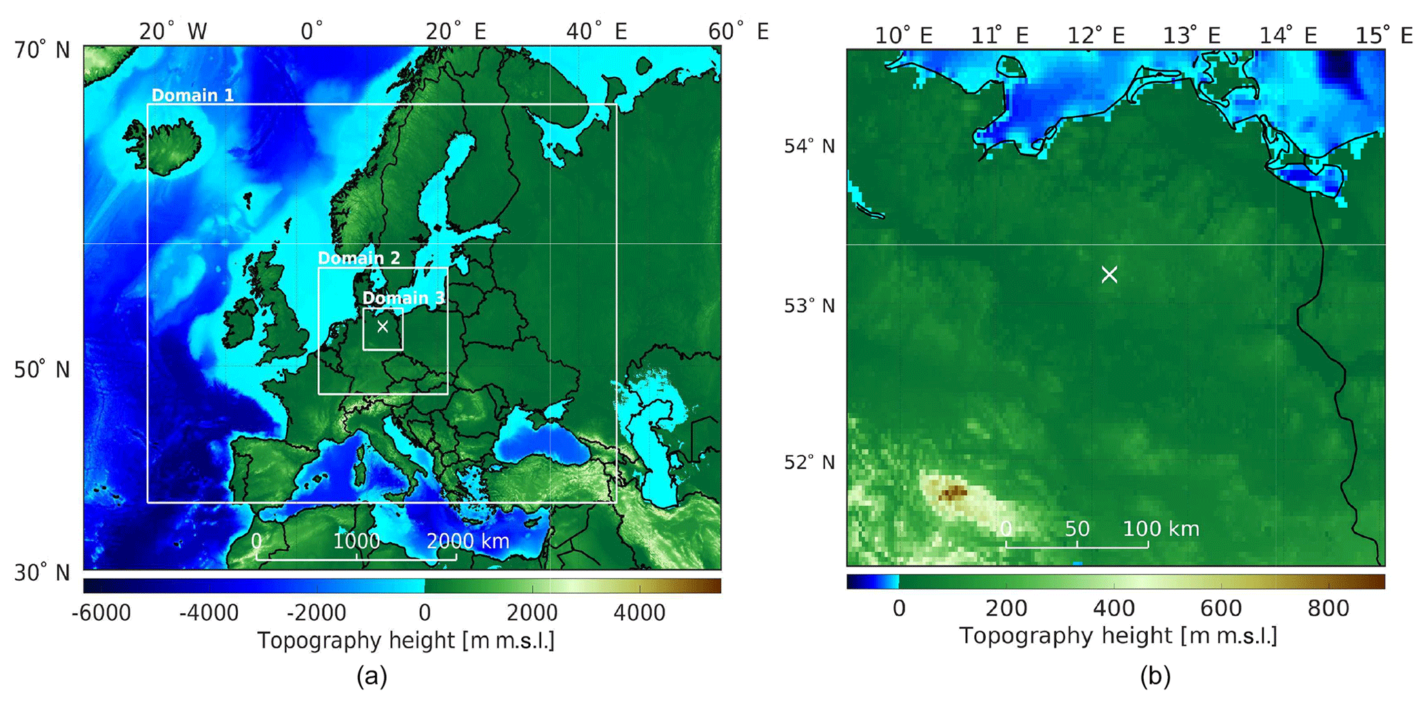
Figure 1 Topography map of all three WRF model domains (a) and a magnification of the innermost domain (b) with the lidar measurement site highlighted by a white X.

Lidar data availability highly depends on the applied carrier-to-noise ratio (CNR) filter and the aerosol content of the air as the wind speed is calculated based on the backscatter of the emitted laser beam. Most aerosols originate from the surface and are transported aloft. Particle density decreases with height and drops to almost zero within the free atmosphere above the ABL (Matthias and Bösenberg, 2002). Data quality quantified by the CNR dropped on average by approximately 5 dB over the course of 1000 m. A fixed CNR threshold of CNR${}_{\mathrm{dB}}>-\mathrm{25}$ dB, combined with additional self-defined filters (Sommerfeld et al., 2019), was applied and insufficient data were discarded. As a result, data availability dropped from about 81 % at 100 m to about 24 % at 1000 m. Low data availability caused by weather effects (e.g., strong precipitation) further emphasizes the importance of simulations for mid-altitude wind resource assessment as no measurement technique with sufficient spatial and temporal resolution is available at this point.

3 Mesoscale modeling framework

To complement the 6-month lidar data set, two WRF 3.6.1 simulations using the Advanced Research Weather Research and Forecasting (ARW) model (Skamarock and Klemp, 2008) were carried out. The “baseline run”, which is hereinafter referred to as NoOBS, is a 12-month study of the area around the measurement location (see Fig. 1) from 1 September 2015 used to derive annual statistics. Lidar measurements (Sommerfeld et al., 2019) were incorporated into the 6-month test model between September 2015 and February 2016 using OBSGRID (Wang et al., 2015), which is hereinafter referred to as OBS.

This methodology uses the difference between the model and measurements to calculate a nonphysical forcing term which is added to the governing conservation equations of the simulation to gradually nudge the model towards the observation (see Eq. 1) (Stauffer et al., 1991; Deng et al., 2007). Each simulation is composed of three nested domains with 27, 9 and 3 km grid spacing and horizontal grid dimensions of about 120×120 elements at 60 heights along the terrain-following vertical hybrid pressure coordinate η. Differences between the simulation runs (see Sect. 3.1) are compared within the innermost domain of the simulation. Output data were stored in 10 min intervals. Figure 1 shows the topography map of the simulation. Initial and boundary conditions of both simulations are based on the ERA-Interim (Dee et al., 2011) reanalysis data set by the European Centre for Medium-Range Weather Forecasts, which consists of 6-hourly atmospheric fields with a spatial resolution of roughly 80 km horizontally and 60η levels. Turbulent kinetic energy (TKE) closure within the ABL was achieved by using the Mellor–Yamada–Nakanishi–Niino (MYNN) 2.5 scheme, which predicts subgrid TKE as a prognostic variable (Nakanishi and Niino, 2004; Lee and Lundquist, 2017). The Noah-MP land-surface model and MYNN surface layer scheme were used. The Rapid Radiative Transfer Model (RRTM) longwave radiation and Dudhia shortwave radiation scheme were used (see Appendix A). In addition to observation nudging (see Sect. 3.1) analysis nudging was performed on every domain of each simulation. Analysis nudging nudges each grid point towards a time-interpolated value from gridded analyses of synoptic observations (Stauffer et al., 1991), whereas observation nudging directly drives the simulation towards the additional observations. Within the planetary boundary layer (PBL) of the inner domain analysis nudging was switched off (see nudging settings in Appendix A). All simulations were run on the EDDY¹ high-performance computing clusters at the University of Oldenburg.

3.1 Observation nudging

Observation nudging, also referred to as “dynamic analysis”, is a form of four-dimensional data assimilation (FDDA) whereby each grid point within the radius of influence and time window is nudged towards observations using a weighted average of differences between the model (q_m interpolated at the observation location) and observations (q_o) (Dudhia, 2012; Reen, 2016). In this study horizontal wind speed U and direction Φ were nudged towards measurements with a time interval of 6 h between an altitude of 66 and 1100 m in order to not overly constrain the simulation. Nudging could not be performed at times and altitudes at which lidar data were not available. The nonphysical forcing term is implemented in the form of prognostic equations (Deng et al., 2007):

$$\begin{array}{}\text{(1)}& \begin{array}{rl}{\displaystyle \frac{\partial q\mathit{\mu }}{\partial t}}& (x,y,z,t)=F_q(x,y,z,t)\\ & +\mathit{\mu }{G}_q{\displaystyle \frac{\sum _{i=\mathrm{1}}^N{W}_q^{\mathrm{2}}(i,x,y,z,t)\left[q_{\mathrm{o}}\left(i\right)-q_{\mathrm{m}}\left(x_i,y_i,z_i,t\right)\right]}{\sum _{i=\mathrm{1}}^N{W}_q(i,x,y,z,t)}}.\end{array}\end{array}$$

Here q refers to the quantity that is nudged, μ is the dry hydrostatic pressure, F_q(x, y, z, t) is the physical tendency term of q, G_q is the nudging strength of q, N is the total number of assimilated observations, i is the index of the current observation, and W_q is the weighting-function-based temporal and spatial separation between grid cells and observations (Dudhia, 2012). The four weighting functions G_q, W_t(x, y, z, t), W_z(x, y, z, t) and W_xy(x, y, z, t) describe the temporal and spatial nudging strength. Values used in this study can be found in Appendix A. The inverse of G_q can be interpreted as a nudging timescale as it dictates how quickly the model approaches the observation.

W_xy and W_z define the spatial nudging weight, while the temporal weighting function W_t defines the duration and weighting strength in time. W_t ramps from 0 to 1 and back to 0 (Reen, 2016). The nudging time window and the time between implemented observations was chosen to be 6 h so that the implemented observations do not overlap each other. This ensures all time steps are nudged while not excessively limiting the model.

Vertical influence was set very small so that observations only affect their own η level (Dudhia, 2012). The horizontal weighting factor W_xy (see Eq. 2) is calculated based on the radius of influence R and the distance between the observation and the grid location D. We used the Cressman scheme as the horizontal nudging weighting function with a radius of influence of R=180 km, thereby affecting the whole inner domain.

$$\begin{array}{}\text{(2)}& w_{xy}=\left\{\begin{array}{ll}\frac{R^{\mathrm{2}}-D^{\mathrm{2}}}{R^{\mathrm{2}}+D^{\mathrm{2}}}& \mathrm{0}\le D\le R\\ \mathrm{0}& \mathrm{else}\end{array}\right.\end{array}$$

4 Results

It is important to keep the differences in temporal and spatial resolution between lidar measurements and WRF simulations in mind. Furthermore, data availability highly influences the ability to nudge the simulation (see Sect. 2) and compare wind speed statistics.

To quantify the local effect of observation nudging, we investigate the cell closest to the lidar measurement location and compare measured and modeled horizontal wind speeds U and direction. Additionally, we investigate several sections at different locations and altitudes within the inner domain to quantify the spatial and temporal impact of single-location observation nudging on the entire domain. Vector values of each WRF cell are calculated on the faces of each cell, linearly interpolated to the cell center and rotated from the grid projection to the earth coordinate system.

4.1 Impact of nudging on wind statistics

Figure 2 shows the scatter plots of measured and simulated horizontal wind speed at various altitudes for times at which lidar data are available. The continuous line represents the linear regression of the data (the regression coefficient is displayed in the legend), while the dotted line shows an ideal correlation. The color of the scatter points corresponds to the frequency of occurrence. Multiple wind speed clusters caused by stratification can be identified. While there is a trend towards higher wind speeds with increasing altitude, low wind speeds (U<6 m s⁻¹) still occur at high altitudes. Both simulations overpredict horizontal wind speeds at low altitudes, which is a known problem of WRF and could be attributed to the model not resolving subgrid-scale roughness elements properly (e.g., modeling a strongly simplified parameterization of forests and/or cities) or flaws in the planetary boundary layer model; this could lead to overly geostrophic winds over land (Mass and Ovens, 2011). Observation nudging improves the overall correlation with measurements at the measurement location as the surface influence decays. Both models approach similar values at higher altitudes, which could be caused by the lack of observations, and therefore observation nudging due to reduced data availability, or is indicative of WRF generally being better at modeling more geostrophic winds.

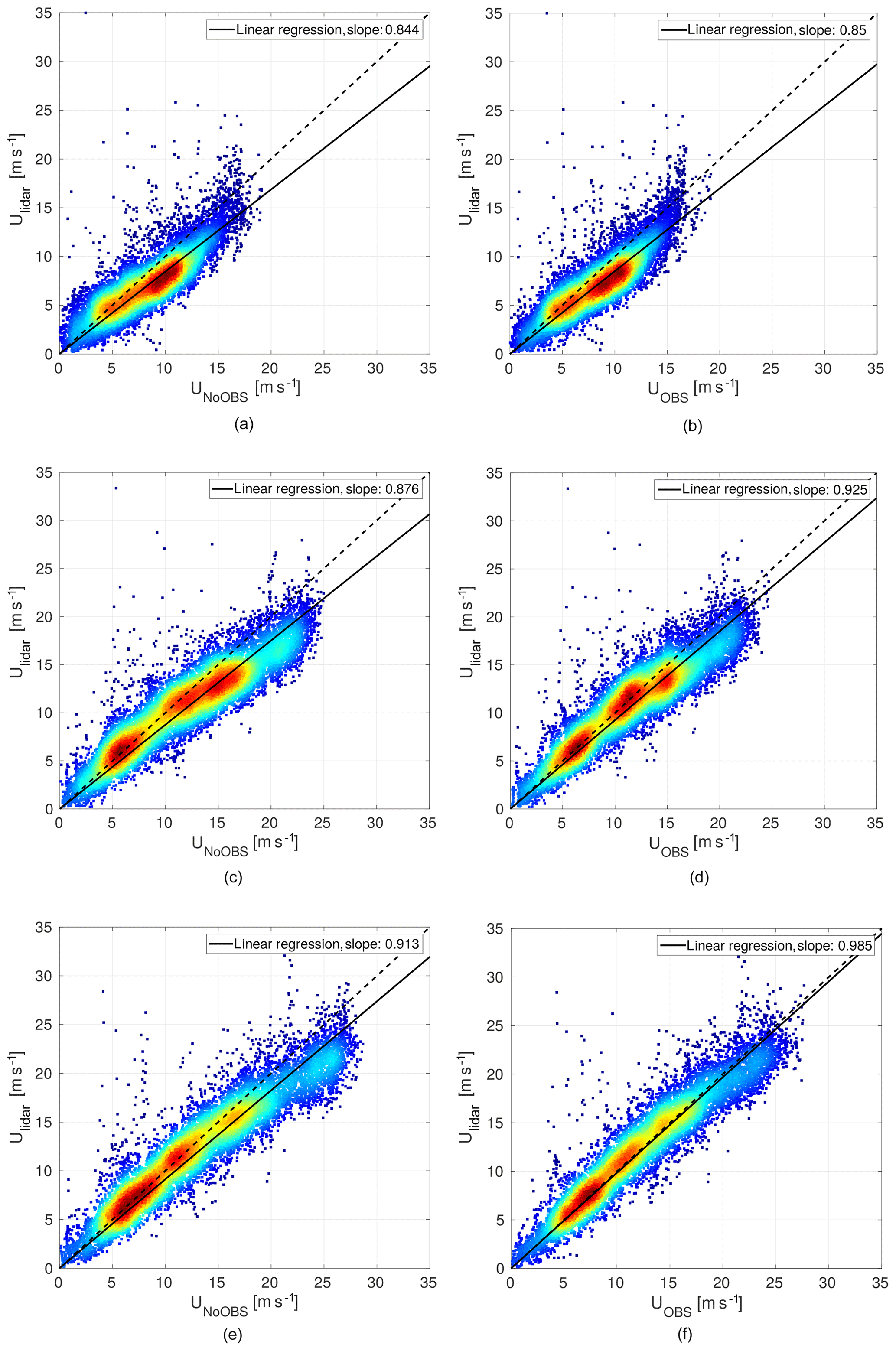
Figure 2 Linear regression of lidar-measured wind speeds against NoOBS-modeled (WRF “baseline run” without observation nudging) wind speeds (a, c, e) and OBS-modeled (“test run” with OBSGRID observation nudging) wind speeds (b, d, f) at ∼100 m (a, b), ∼300 m (c, d) and ∼500 m (e, f).

The statistical analysis of the absolute difference between the WRF-simulated quantities at the measurement location and the lidar observations ($\mathrm{\Delta }U=U_{\mathrm{WRF}}-U_{\mathrm{lidar}}$; $\mathrm{\Delta }\mathrm{\Phi }={\mathrm{\Phi }}_{\mathrm{WRF}}-{\mathrm{\Phi }}_{\mathrm{lidar}}$ wrapped on an interval [−π, π]) is shown in Fig. 3 in the form of a box plot. The circle corresponds to the median, the colored box indicates the 25th and 75th percentile, and the whiskers to both sides mark ±2.7 times the standard deviation (σ). Outliers beyond ±2.7σ are hidden to maintain clarity and readability. The continuous line in Fig. 3a represents the root mean square error between the measured U_lidar and simulated wind speed U_WRF.

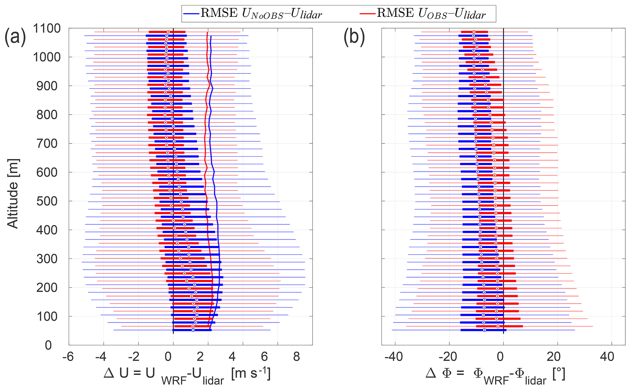
Figure 3 Statistical analysis of the bias between simulated and measured wind speed (ΔU) and direction bias (ΔΦ). The circle corresponds to the median, the colored box indicates the 25th and 75th percentile, and the whiskers mark ±2.7σ. The solid lines in (a) show the RMSE between the modeled and measured wind speed.

The simulation with observation nudging generally outperforms the unnudged simulation and is in better agreement with the measurements, particularly at the altitudes of interest to high-altitude wind energy systems. It furthermore reduces the spread of the bias, illustrated by the smaller whiskers and boxes. The root mean square error (RMSE) ΔU shows similar results for both simulations below 100 m and above 700 m. The largest improvement or smallest error can be found between 300 and 600 m. This could be explained by a better performance of the mesoscale model at these altitudes due to a reduced impact of the air–surface interaction, which is strongly parameterized.

The NoOBS shows an almost constant wind direction bias at all altitudes. Observation nudging substantially reduces the directional bias ΔΦ up to high altitudes as can be seen in Fig. 3b. Similar to the wind speed bias, wind direction bias at 1100 m is almost the same for both simulations. The negative wind direction bias represents an anticlockwise deviation. Other studies (Carvalho et al., 2014; Giannakopoulou and Nhili, 2014) have found similar wind direction biases. A possible reason for this systematic error is that WRF does not adequately resolve surface roughness, resulting in lower surface friction and leading to overly geostrophic winds (Mass and Ovens, 2011). The almost constant median wind direction bias indicates that WRF is able to capture the clockwise rotation of the “Ekman spiral” in the Northern Hemisphere.

4.2 Representative nudging results

We compare 10 min mean horizontal wind speed for 24 h on 21 September 2015 in Fig. 4 to visualize the impact of observation nudging on the mesoscale model output. The white spaces in the lidar measurements (see Fig. 4a) are data points that have been filtered out due to insufficient data quality. The dashed line is the WRF-modeled surface heat flux (SHF) used to estimate atmospheric stability (see Sect. 4.5). The color of the profiles indicates the wind direction, and lidar-measured profiles are shown in grey for comparison. The black dot in each profile marks the altitude of highest wind speed, while the black circle indicates the optimal altitude for the operation of an airborne wind energy system based on a simplified power approximation (see Sect. 4.7). However, the single-point representation is only a rough measure of operational altitude since an AWES generally sweeps a range of altitudes.

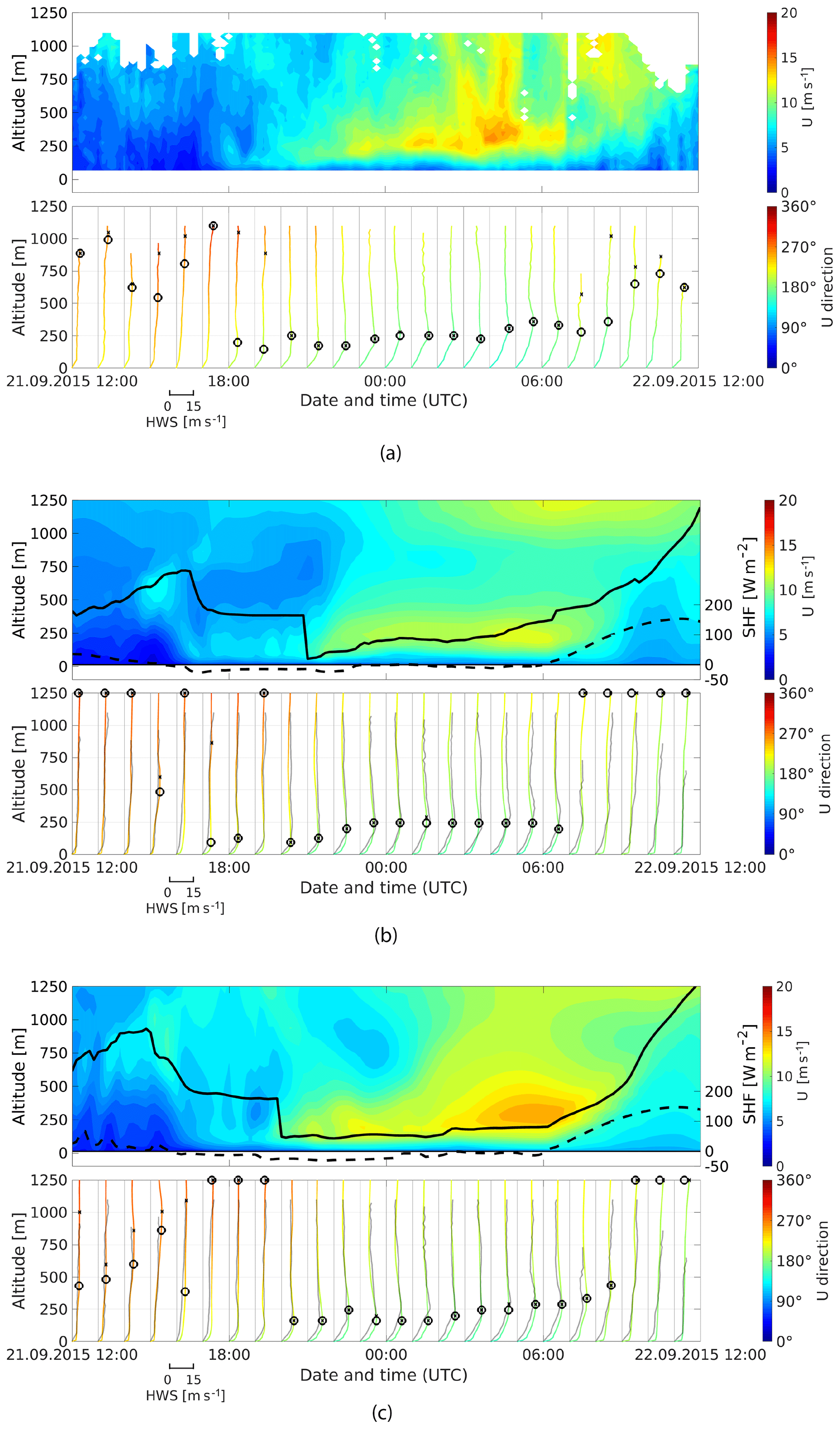
Figure 4 Visualization of modeled and measured 10 min mean wind speed and wind direction for 21 September 2015. (a) The measured lidar data set, (b) the observation-nudged OBS data set and (c) results from the unnudged reference NoOBS model. (a) The wind speed and WRF-calculated SHF (dashed line). (c) The hourly 10 min mean wind speed profile colored according to wind direction. X marks the altitude of highest wind speed and ◦ the optimal AWES operating altitude calculated as described in Sect. 4.7.

Even though observation nudging leads to statistical improvements in wind speed and wind direction prediction over the entire period (compare Sect. 4.1 and 4.4), individual days can still show a decline in model accuracy. The low-level jet (LLJ) and high wind speeds at higher altitudes, which the NoOBS model captures fairly well, are significantly weaker in the OBS model. Implementing additional measurements at a higher frequency might yield results closer to measurements, but adding too many unphysical forcing terms might overly restrict the simulation.

The planetary boundary layer height (PBLH) (black line), which in the MYNN scheme is calculated from the profile of virtual potential temperature and from the profile of the TKE (Brunner et al., 2015; Nakanishi and Niino, 2004), is directly affected by wind speed observation nudging. During the investigated day, observation nudging leads to a lower daytime PBLH.

4.3 Spatial influence

Single-location observation nudging influences the area within the radius of influence (R_xy=180 km; see Appendix A), which here includes the entire inner domain (150 km × 150 km). Figure 5 shows the mean absolute difference of horizontal wind speed ($\mathrm{\Delta }U=\left|U_{\mathrm{OBS}}\right|-\left|U_{\mathrm{NoOBS}}\right|$) between the OBS and NoOBS model along lines of constant longitude and latitude for the entire simulation period. The grid cell in which observations were assimilated is indicated by the vertical line and highlighted by the square marker. The four colors indicate different altitudes. As the outer domains remain unnudged, the boundary conditions of the inner domain remain the same, which leads to a rapid decline in absolute difference towards the outside of the domain. The difference in wind speed does not go to exact zero because the results are interpolated to the center of each grid cell. Near-surface results close to the measurement location, which is highlighted by the black vertical line, experience the largest change in wind speed (red line, z=12 m). The asymmetry could be caused by the downstream transportation of nudging effects (dominant wind direction: west).

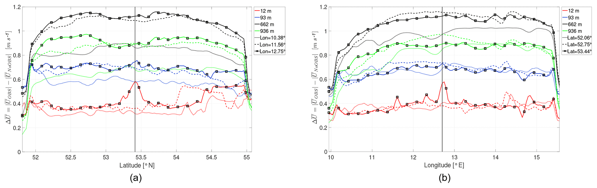
Figure 5 Mean absolute wind speed difference $\mathrm{\Delta }\stackrel{\mathrm{‾}}{U}$ along lines of constant longitude (a) and latitude (b) within the inner, nudged WRF domain. Approximate distance of d₃≈180 km (dotted lines), d₂≈75 km (dashed lines) and d₁≈0 km (solid line) from the center (lat: 53^∘10^′47.00^′′ N, lon: 12^∘11^′20.98^′′ E) where the OBS model was nudged. The vertical line highlights the grid cell closest to the observation.

4.4 Diurnal variability

Average diurnal variation indicates typical wind speed variations for a given location and period. It further reinforces the benefit of dynamically adapting operating altitudes of AWES. The hourly average lidar wind speed depends on data availability, as described in Sect. 2. Lidar availability below 100 m on average decreases by about 10 percentage points during the noon hours, while it remains fairly constant at altitudes between 100 and 300 m. Above this altitude, data availability increases in the afternoon by up to about 15 percentage points (Sommerfeld et al., 2019).

Figure 6a shows the lidar-measured and mesoscale modeled diurnal wind speed variation at the measurement location filtered by lidar availability; i.e., times when no lidar data were available were disregarded. A clear diurnal wind speed variation resulting from the cycle of stable and unstable stratification can be identified. On average OBS shows lower hourly wind speeds than NoOBS and is closer to measurements. The diurnal variation of the unfiltered 12-month NoOBS, 6-month OBS and 6-month NoOBS data sets (Fig. 6, right) deviates significantly from the measurements. Observation nudging leads to overall lower wind speeds and wind shear throughout the day in the unfiltered data set. Due to the large difference in average measured and unfiltered modeled diurnal wind speeds, it seems that lidar measurements alone cannot appropriately represent average wind conditions aloft due to availability bias, which has also been observed at other locations (Gryning and Floors, 2019). Therefore, we believe that the nudged data set yields more representative results than the unnudged model or the measurements alone.

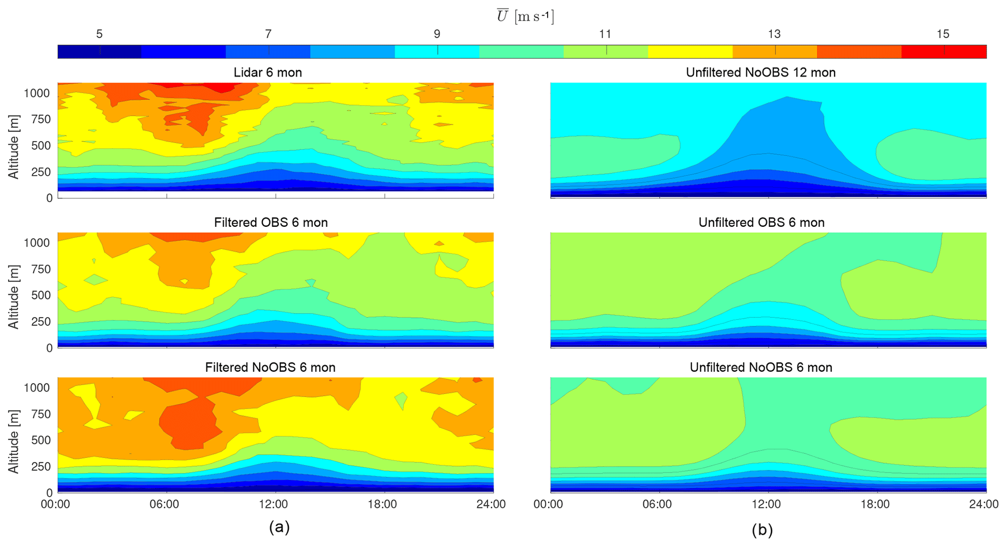
Figure 6 Hourly average diurnal variation of measured and modeled horizontal wind speed $\stackrel{\mathrm{‾}}{U}$ filtered by lidar availability (a) and unfiltered (b).

4.5 Wind speed probability distribution

The common way to approximate the probability distribution of the horizontal wind speed f(U) is the Weibull distribution fit (Eq. 3), which describes the statistical distribution as a function of the scale parameter A and the shape parameter k (Troen and Lundtang Petersen, 1989).

$$\begin{array}{}\text{(3)}& f_{\mathrm{Weibull}}\left(u\right)={\displaystyle \frac{k}{A}}{\left({\displaystyle \frac{u}{A}}\right)}^{k-\mathrm{1}}{e}^{-{\left(\frac{u}{A}\right)}^k}\end{array}$$

Previous investigation of the lidar measurements showed a multi-modality in the wind speed frequency of occurrence caused by different atmospheric stability (Sommerfeld et al., 2019). Figure 7a visualizes the entire measured and simulated wind speed frequency distribution. Its corresponding Weibull fit is shown in Fig. 7b, and the difference between the two can be found in Fig. 7c. Each row summarizes the various data sets: first 6-month lidar, then 6-month OBS and 6-month NoOBS, followed by 12-month NoOBS.

Figure 7 Frequency of occurrence (a), Weibull fit (b) and difference between the two (c) for the 6-month lidar measurements (top row), 6-month OBS model (second row), 6-month NoOBS model (third row) and 12-month NoOBS (bottom row). All data (not filtered by lidar data availability) were used for the WRF data set.

All 6-month data sets show a high occurrence of low and high wind speeds, which indicates a multi-modal frequency distribution. This effect is most pronounced in the lidar data set. The comparison of wind speed frequency with the Weibull fit further emphasizes the multi-modality as a simple Weibull fit is not able to capture the higher probability at low and high wind speeds. These distinct flow situations further drift apart with increasing surface distance. As a result the Weibull distribution overestimates the occurrence of wind speeds between the two peaks. Both OBS and NoOBS slightly overestimate low-altitude wind speed (see Fig. 3) compared to lidar measurements. Both models and the lidar measurements show a broadening of the frequency distribution towards higher altitudes. High wind speeds become more likely, while low wind speeds still occur. Therefore, an AWES needs to be able to operate in a wide range of wind speeds or be controlled in a way that avoids extreme conditions. The 12-month NoOBS simulation shows lower wind speeds than the 6-month simulations as the included summer months generally have lower wind speeds due to the lower synoptic pressure gradients. The Weibull fit of this simulation tends to overestimate higher wind speeds and underestimate low wind speeds at all altitudes.

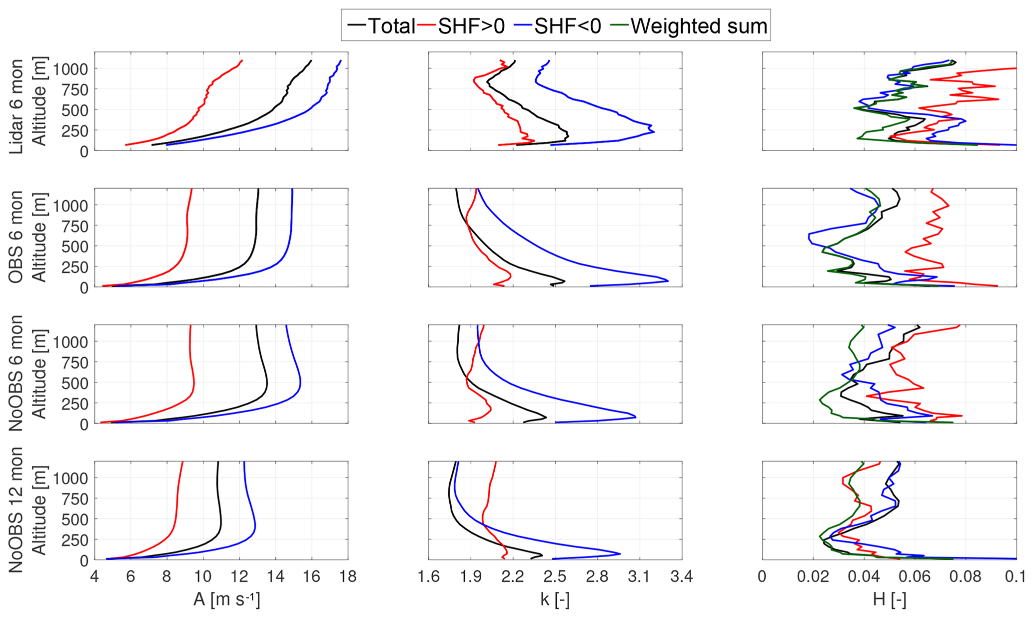
Figure 8 Weibull parameter trends over altitude and goodness of fit quantified by the Hellinger distance (right) over altitude for 6 months of lidar measurements (first row panels), the 6-month OBS model (second row panels), 6-month NoOBS model (third row panels) and the 12-month NoOBS model (fourth row panels).

Using the sign of the WRF-calculated SHF as a simple proxy to differentiate stable and unstable wind conditions similar to Sommerfeld et al. (2019), the wind speed distribution follows the expected trends of low wind shear during unstable stratification and higher wind shear and wind speeds during stable stratification (Arya and Holton, 2001). Observation nudging reduces the occurrence of high wind speeds at high altitudes in comparison to NoOBS and leads to an increase in the probability of wind speeds around 5 m s⁻¹ during times of positive SHF. The Weibull distribution fit of these sub-states is generally better at representing the modeled wind conditions.

Figure 8 shows the scale parameter A, shape parameter k and Hellinger distance H (Upton and Cook, 2008) between the wind speed frequency distribution and the corresponding Weibull distribution fit for lidar (first row), 6-month OBS (second row), 6-month NoOBS (third row) and 12-month NoOBS (fourth row).

The different trends under positive and negative SHF of both Weibull parameters visualize the existence of entirely different flow regimes. The Hellinger distance between the Weibull fit and frequency distribution (negative SHF: blue, positive SHF: red), the total data and a simple fit (black), and between the total data and the weighted sum of both Weibull fits (green) is shown. All WRF models show an overall smaller H than a similar analysis of the lidar data set (Sommerfeld et al., 2019). The sharp bend in both A and k of the lidar data above 750 m is likely caused by insufficient data availability. NoOBS results show a sharp increase in A up to 250 m and a slight reduction above, while OBS shows a trend close to the surface, and A values remain almost constant above 500 m. No data set shows a convergence of A at higher altitudes, indicating that these wind conditions are driven by different conditions in the free atmosphere. The 12-month NoOBS simulations show lower-scale parameter values as they include generally slower winds during summer. While A trends are quite different for lidar and WRF, k trends are more similar. They peak between 150 and 250 m and are especially high during stable stratification (Monahan et al., 2011). OBS trends of k are generally closer to measurement results than NoOBS.

Even though the Hellinger distance of individual Weibull fits for times of positive or negative SHF is generally higher than the Weibull fit of the entire data set, the weighted sum of both individual fits yields the best result at all altitudes. The 12-month Weibull fit using the entire data set performs comparably to a weighted sum up to an altitude of about 250 m.

4.6 Effect of stability on average wind shear

Atmospheric stability highly influences the shape of wind speed profiles, which is important for determining optimal operating conditions for an AWES (see Sect. 4.7). Obukhov length L (Obukhov, 1971; Sempreviva and Gryning, 1996) is commonly used to categorize the stability of the boundary layer. Here the application is extended to mid-altitudes. L is defined by the simulated friction velocity u_*, virtual potential temperature θ_v, potential temperature θ, kinematic virtual sensible surface heat flux Q_S, kinematic virtual latent heat flux Q_L, the von Kármán constant k and gravitational acceleration g. Table 1 summarizes the frequency of occurrence of each stability class.

$$\begin{array}{}\text{(4)}& L=\left({\displaystyle \frac{-u_{*}^{\mathrm{3}}{\mathit{\theta }}_{\mathrm{v}}}{kg}}\right)\left({\displaystyle \frac{\mathrm{1}}{Q_{\mathrm{S}}}}+{\displaystyle \frac{\mathrm{0.61}}{Q_{\mathrm{L}}\mathit{\theta }}}\right)\end{array}$$

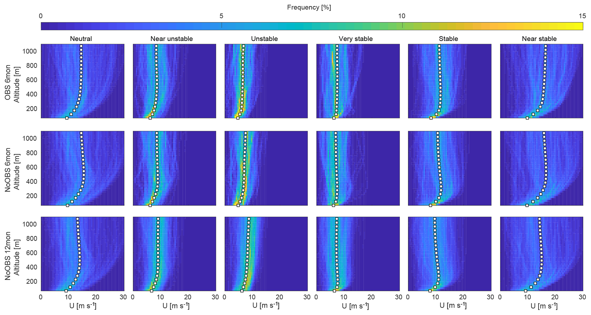
Figure 9 Wind speed U, frequency of occurrence and mean (white square) categorized by atmospheric stability according to Obukhov length L (see Table 1) for 6-month OBS (top panels), 6-month NoOBS (center panels) and 12-month NoOBS (bottom panels).

Table 1 Stability classes according to Obukhov length calculated based on WRF results (Floors et al., 2011).

In comparison with the unnudged simulation, OBS shows an increase in unstable and nearly unstable situations. Stable and nearly stable stratification seem almost unaffected by OBS nudging, while neutral and very stable stratification occur slightly less often. This might improve the overall predicting capabilities of WRF as the MYNN 2.5 boundary layer scheme overestimates the frequency of very stable conditions with an error of up to 9 % (Krogsæter and Reuder, 2015). Neutral conditions, still commonly used in many wind energy siting applications, only occur about 30 % of the time during the measurement period and only about 20 % of the time during the 1-year reference NoOBS simulation.

Figure 9 shows the frequency distribution of the different stability categories with the mean highlighted by white squares. All categories show distinct trends and distributions that are consistent between data sets, which contribute to the multi-modality of the overall wind speed frequency distribution. The difference in high-altitude wind speeds between stratifications indicates the influence of different geostrophic wind conditions. The categorization by L is based on surface data and seems to be valid within the lower part of the atmosphere where the spread of the corresponding frequency distribution is relatively small in comparison to high altitudes. This is particularly true for stable and neutral stratification whereby wind speeds above approximately 200 m spread widely. Unstable conditions are probably more consistent because of increased mixing from the surface up to high altitudes. The divergence of wind speeds towards higher altitudes indicate inhomogeneous atmospheric stability and suggests that surface-based stability categorization is insufficient for higher altitudes. Wind speed extrapolation based on low-altitude measurements can lead to a misestimation of mid-altitude wind conditions, especially during neutral and stable conditions close to the surface (Konow, 2015).

Altitudes below 200 m are least affected by observation nudging as OBS remains almost unchanged from NoOBS (see Sect. 4.1). Stable profiles show a peak at around 300 m, which is indicative of a characteristic low-level jet. Comparing OBS and NoOBS for 6 months, observation nudging seems to reduce the spread at higher altitudes within each category except very stable. The impact of observation nudging on wind profiles during unstable stratification is relatively low, while wind speed profiles under neutral and stable stratification are more affected.

4.7 Optimal operating altitude and power production

We estimate optimal operating altitude and traction power of a ground-generator AWES using a simple ground-generator (pumping-mode) AWES point-mass model adapted from Schmehl et al. (2013). We focus on 6-month OBS, as we previously proved increased accuracy, and use 12-month NoOBS to estimate annual values. The estimated optimal power per unit of lifting area of the wing p_opt is described by

$$\begin{array}{}\text{(5)}& \begin{array}{rl}{p}_{\mathrm{opt}}=& {\displaystyle \frac{{\mathit{\rho }}_{\mathrm{air}}}{\mathrm{2}}}{U}^{\mathrm{3}}\sqrt{c_{\mathrm{L}}^{\mathrm{2}}+c_{\mathrm{D}}^{\mathrm{2}}}\left[\mathrm{1}+{\left({\displaystyle \frac{c_{\mathrm{L}}}{c_{\mathrm{D}}}}\right)}^{\mathrm{2}}\right]\\ & f_{\mathrm{opt}}{\left(\cos \mathit{\epsilon }\cos \mathit{\varphi }-f_{\mathrm{opt}}\right)}^{\mathrm{2}}={\displaystyle \frac{\mathrm{2}}{\mathrm{27}}}{\mathit{\rho }}_{\mathrm{air}}{U}^{\mathrm{3}}\\ & \sqrt{c_{\mathrm{L}}^{\mathrm{2}}+c_{\mathrm{D}}^{\mathrm{2}}}\left[\mathrm{1}+{\left({\displaystyle \frac{c_{\mathrm{L}}}{c_{\mathrm{D}}}}\right)}^{\mathrm{2}}\right]\cos {\mathit{\epsilon }}^{\mathrm{3}}.\end{array}\end{array}$$

Air density ρ_air is calculated by a linear approximation of the standard atmosphere (, ) (ρ_air(z)=1.225–0.00011z; kg m⁻³). Losses associated with the mispositioning of the aircraft relative to the wind direction, expressed by azimuth angle ϕ and elevation angle ε relative to the ground station, are included in the model. Additional losses caused by gravity, tether sagging and tether drag are neglected. As a result, lift F_L and drag F_D force and therefore the lift (c_L=1.7) and drag coefficients (c_D=0.06), which are assumed to be constant, are geometrically related to the apparent wind velocity. Assuming an optimal tether speed and a quasi-steady state with the wing moving directly cross-wind with a zero azimuth angle (ϕ=0) relative to the wind direction, we can estimate the optimal traction power. The optimal elevation angle (ε_opt) and operating altitude (z_opt) are geometrically related to the assumed-constant tether length (l_tether) ($\sin {\mathit{\epsilon }}_{\mathrm{opt}}=\frac{z_{\mathrm{opt}}}{l_{\mathrm{tether}}}$).

Figure 10 summarizes the frequency of optimal operating altitude and optimal power assuming a constant tether length of 1500 m. The white solid line shows the cumulative frequency of optimal operating altitude. Both simulations for this particular location and time period show similar trends, with the most probable optimal altitude between approximately 200 and 400 m. Times of very high traction power are fairly rare and likely associated with low-level jets. Lower power at higher altitudes is caused by misalignment losses.

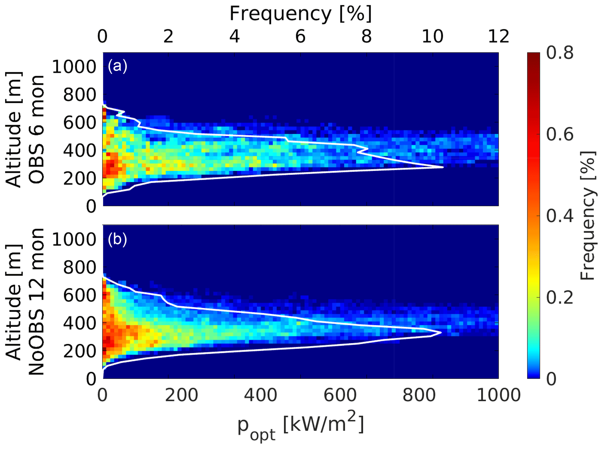
Figure 10 Frequency of optimal traction power over optimal operating altitude based on 6-month OBS (a) and 12-month NoOBS (b) assuming a constant tether length of 1500 m. The continuous white line shows the frequency of optimal operating altitude for the whole power range (abscissa axis in a).

Figure 11 estimates the optimal traction power and operating altitude as a function of tether length based on the mean wind speed profile of atmospheric stability conditions (Fig. 9). The tether length of each estimation is assumed to be constant and used to calculate the optimal elevation angle. The axis limits of different atmospheric conditions had to be adjusted as the calculated power varied by orders of magnitude. All estimates show diminishing benefits of a longer tether. These incremental gains would probably be negated by additional drag- and weight-associated losses. Winds during times of very stable and unstable stratification lead to a clear optimal altitude independent of tether length between 200 and 400 m, while weakly stable and shear-driven wind speed profiles lead to higher optimal operating altitudes and a broader range of optimal altitudes as a function of tether length.

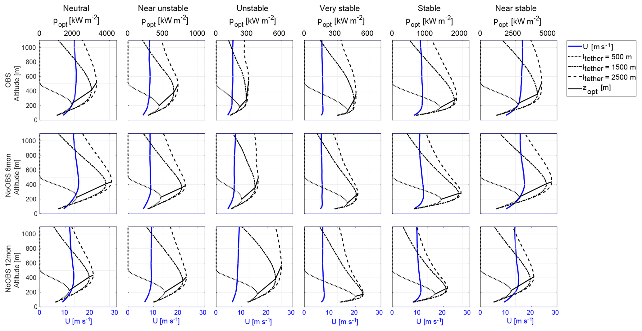
Figure 11 Optimal traction power per wing area p_opt (dashed lines) and optimal operational altitude (solid line) estimated based on mean wind speed profiles categorized by Obukhov length (L) for 6-month OBS, 6-month NoOBS and 12-month NoOBS simulations with varying tether length (l_tether=500–2500 m).

5 Conclusion

A full 6 months of lidar measurements up to 1100 m were assimilated into a mesoscale model using observation nudging. An unnudged reference model (NoOBS), the nudged model (OBS) outputs and lidar measurements were compared in terms of wind speed and direction statistics, as well as wind profile shape at the measurement site, and spatial differences were quantified. Observation nudging only has a marginal impact on simulated surface layer wind speeds as ground effects dominate the WRF model. Wind speeds between 300 and 500 m were most affected by observation nudging. Modeled wind speeds at these altitudes are statistically closest to the measurements, making this an adequate approach for resource assessment at mid-altitudes as measurement availability decreases. The impact of nudging weakens above these altitudes. Whether this is caused by lower measurement data availability or a generally better performance of the mesoscale model above the surface layer could not be determined. Observation nudging reduced the seemingly systematic wind direction bias between simulations and measurements at all altitudes. Due to the lack of high-resolution measurements at high altitudes, unnudged mesoscale model data are the best we have in terms of preliminary resource assessment.

Filtering the mesoscale model data according to lidar data availability yields similar diurnal variation, with OBS being closer to measurements. Comparing the diurnal variation of the unfiltered model wind speeds to measurements shows a significant deviation, which is likely caused by insufficient lidar data availability at higher altitudes. The bias between real and lidar-measured wind speed, which depends on the applied CNR threshold and data availability, can result in a misrepresentation of the actual wind conditions, especially at higher altitudes. Mesoscale models, particularly with observation nudging, can be used to account for this error. Lidar measurements seem to be biased towards high wind speeds as measured winds are generally higher than the unfiltered mesoscale model data. The impact of observation nudging on the wind profiles in the case of an unstably stratified boundary layer is relatively low, while wind speed profiles under stable stratification are significantly affected. At the measurement location OBS is overall closer to measurements, especially between 200 and 600 m. Variations of stratification, primarily those associated with the diurnal cycle, lead to a multi-modal wind speed frequency distribution which is better represented by the weighted sum of two Weibull fits than by a single Weibull fit. Obukhov-length-categorized wind speed profiles, especially during neutral and stable conditions close to the surface, show a divergence with height. This indicates inhomogeneous atmospheric stability and suggests that surface-based stability categorization is insufficient for higher altitudes.

Optimal AWES operating altitudes and power output per wing area were estimated based on a simplified model for 6 months of OBS and 12 months of NoOBS. The model neglects kite and tether weight as well as tether drag. Accounting for these losses, which are proportional to tether length, will reduce the performance of the AWES. Results for both wind speed data sets show the highest potential at an altitude between 200 and 600 m above which the losses associated with the elevation angle are too high. A comparison of different tether lengths under average wind speeds associated with different atmospheric stability conditions shows diminishing returns in terms of power output for tether lengths longer than 1500 m. While higher altitudes can potentially be reached, the optimal operating altitude remains almost unchanged. The highest energy potential and operating altitude is associated with neutral and stable stratification. Unstable conditions result in significantly lower energy potential due to lower, almost altitude-independent average wind speeds.

Future studies will include using the enhanced mesoscale model output to drive large-eddy simulations to provide better insight into mid-altitude turbulence. The resulting data set will lead to the development of a mid-altitude engineering wind model which can be used for the design, load estimation, control and optimization of airborne wind energy systems. Mesoscale model data will be implemented into an AWES optimization framework to quantify the impact of various wind speed profiles on power production, optimal trajectory and system size. Furthermore, the possibility of merging the mesoscale output with lidar measurements to fill gaps in the measurement data set to reduce the wind speed bias introduced by lidar availability is being investigated.

Appendix A: Namelist parameters for WRF 3.6.1 observation nudging

WRF input parameter	Value
grid_fdda	1, 1, 1,
gfdda_inname	“wrffdda_d<domain>”,
gfdda_end_h	99 999, 99 999, 99 999,
gfdda_interval_m	360, 360, 360,
fgdt	0, 0, 0,
if_no_pbl_nudging_uv	0, 0, 1,
if_no_pbl_nudging_t	0, 0,1,
if_no_pbl_nudging_q	0, 0, 1,
if_zfac_uv	0, 0, 0,
k_zfac_uv	0, 0, 30,
if_zfac_t	0, 0, 0,
k_zfac_t	0, 0, 30,
if_zfac_q	0, 0, 0,
k_zfac_q	0, 0, 30,
guv	0.0003, 0.0003, 0.0003,
gt	0.0003, 0.0003, 0.0003,
gq	0.0003, 0.0003, 0.0003,
if_ramping	1,
dtramp_min	60.0,
io_form_gfdda	2,
obs_nudge_opt	0,0,1
Cressman scheme	1
time_step	60
obs_rinxy	240, 240, 180
obs_rinsig	0.1
obs_twindo	3, 3, 3
auxinput11_interval_s	360, 360, 360
obs_dtramp	40
obs_nudge_wind	1, 1, 1
obs_coef_wind	$\mathrm{6}\times {\mathrm{10}}^{-\mathrm{4}}$, $\mathrm{6}\times {\mathrm{10}}^{-\mathrm{4}}$, $\mathrm{6}\times {\mathrm{10}}^{-\mathrm{4}}$
iobs_onf	2, 2, 2
auxinput11_interval_s	360, 360, 360
auxinput11_end_h	6, 6, 6
if_no_pbl_nudging_uv	0, 0, 1
if_zfac_uv (max_dom)	0, 0, 30
sf_sfclay_physics	5, 5, 5
sf_surface_physics	4, 4, 4
bl_pbl_physics (max_dom)	5, 5, 5
bl_mynn_tkeadvect	.true., .true., .true.
ra_lw_physics	1, 1, 1
ra_sw_physics	1, 1, 1
mp_physics	5, 5, 5