the Creative Commons Attribution 4.0 License.
the Creative Commons Attribution 4.0 License.
 | 28 Jan 2019
Determination of natural frequencies and mode shapes of a wind turbine rotor blade using Timoshenko beam elements
Evgueni Stanoev
Sudhanva Kusuma Chandrashekhara
When simulating a wind turbine, the lowest eigenmodes of the rotor blades are usually used to describe their elastic deformation in the frame of a multi-body system. In this paper, a finite element beam model for the rotor blades is proposed which is based on the transfer matrix method. Both static and kinetic field matrices for the 3-D Timoshenko beam element are derived by the numerical integration of the differential equations of motion using a Runge–Kutta fourth-order procedure. In the general case, the beam reference axis is at an arbitrary location in the cross section. The inertia term in the motion differential equation is expressed using appropriate shape functions for the Timoshenko beam. The kinetic field matrix is built by numerical integration applied on the approximated inertia term. The beam element stiffness and mass matrices are calculated by simple matrix operations from both field matrices. The system stiffness and mass matrices of the rotor blade model are assembled in the usual finite element manner in a global coordinate system accounting for the structural twist angle and possible pre-bending. The program developed for the above-mentioned calculations and the final solution of the eigenvalue problem is accomplished using MuPAD, a symbolic math toolbox in MATLAB®. The natural frequencies calculated using generic rotor blade data are compared with the results proposed from the FAST and ADAMS software.
- Article
(1336 KB) - Full-text XML
- BibTeX
- EndNote


Vibration of an elastic system refers to a limited reciprocating motion of a particle or an object of the system. Wind turbines operate in an unsteady environment which results in a vibrating response (see Manwell et al., 2009). They consist of long slender structures (rotor blades and tower), which result in resonant frequencies that should be taken into account during the initial design and construction. When the excitation frequency of the vibrating system is near any natural frequency, an undesirable resonant state occurs with large amplitudes, which may lead to damage or even the collapse of the wind turbine or its components. The vibration response, especially of the rotor blades, depends on the stiffness which is a function of the materials used, the design and the size (see Jureczko et al., 2005). Therefore, the estimation of natural frequencies in the early design phase plays an important role in avoiding resonance.
The eigenmodes associated with the lowest natural frequencies are employed as shape functions to describe the elastic deformation of the rotor blade beam model in the frame of the usual simulation of the wind turbine as a multi-body system. Generally, the first two bending eigenmodes in each direction (flapwise and edgewise) and optionally the two additional torsional eigenmodes are used. The determination of the lowest eigenmodes with sufficient numerical accuracy is the first step with respect to the modal superposition applied to the deformational motion of the rotor blades.
Due to the geometrical complexity of the blade cross section profiles and the extended use of composite materials, the exact calculation of natural frequencies in the design process takes a considerable amount of time and financial expense with regards to the 3-D modelling of the rotor blade using CAD software; hence a simplified finite element beam model is necessary. A twisted rotor blade is simplified into a cantilever beam with a non-uniform cross section. The structural twist angle is implemented by changing the orientation of the principal axis of the blade cross section along the length of the blade.
In the finite element formulation of beams two linear beam theories are established, the Euler–Bernoulli beam model and the Timoshenko beam model. Although the Euler–Bernoulli beam theory is widely used, the Timoshenko beam theory is considered to be better as it incorporates the effects of transverse shear and the rotational inertia on the dynamic response of the beam (see Kaya, 2006). In the classical approach of the finite element formulation for the free vibration analysis of beams, the stiffness and mass matrices are derived using interpolation functions derived from second- and fourth-order Hermite polynomials. The stiffness matrix is derived from the following equation (see Wu, 2013):
where K(e) is the element stiffness matrix, B is the strain matrix and Dm is the elasticity matrix for the beam. The element mass matrix of the beam (see Wu, 2013) is derived using the following equation:
where M(e) is the element mass matrix, ρ is the mass density, v is the volume and a is the matrix of interpolation functions.
Using the above-mentioned standard relations and appropriate shape functions for the Euler–Bernoulli beam and the Timoshenko beam, the stiffness matrix and consistent mass matrix for the finite beam element can be derived. However, an alternative to this procedure, based on the transfer matrix method for the beam theory (see Graf and Vassilev, 2006:69–88 and Stanoev 2007) is developed in the present article. The element stiffness matrix can be derived on the basis of numerical integration of the first-order ordinary differential equation system for the differential beam element. The associated mass matrix can be developed by numerical integration of the inertia term in the differential equation of motion. The numerical integration results in static and kinetic field matrices, from which the element stiffness and mass matrices can be easily assembled.
In the present article, the above-mentioned procedure is used to determine the element stiffness and element mass matrix for the Timoshenko beam. The interpolation functions used for deriving the mass matrix are based on Hermite polynomials according to Bazoune and Khulief (2003). The system stiffness and mass matrices for the rotor blade are assembled in a global coordinate basis in the usual finite element manner. The numerical solution of the associated eigenvalue problem for the system without damping is computed using computer algebra software (in the frame of MATLAB®).
In Sects. 2 and 3, the proposed method is described in detail; in Sect. 4 the method is applied on a rotor blade structure with 288 degrees of freedom (DOFs). The results for the natural frequencies and the corresponding eigenmodes are compared with the results calculated using the FAST and ADAMS software.
2.1 Kinematic relationships
The general assumptions in the linear beam theory are as follows:
- a.
The beam reference (longitudinal) axis is at any arbitrary location of the cross section.
- b.
The only stresses that occur are normal stresses σx and shear stresses τxy, τxz.
- c.
Cross section planes, which are initially normal to the longitudinal axis, will remain plane after deformation.
The geometrical representation of the deformation state of a beam cross section is shown in the Fig. 1. The deformations up, vp and wp at a cross-sectional point P are determined by three displacement functions u(x), v(x) and w(x) and three cross-sectional rotation angles φx(x), φy(x) and φz(x) – all of them are a function of the beam axis coordinate x. The differential equation system is derived in accordance with Stanoev (2013):
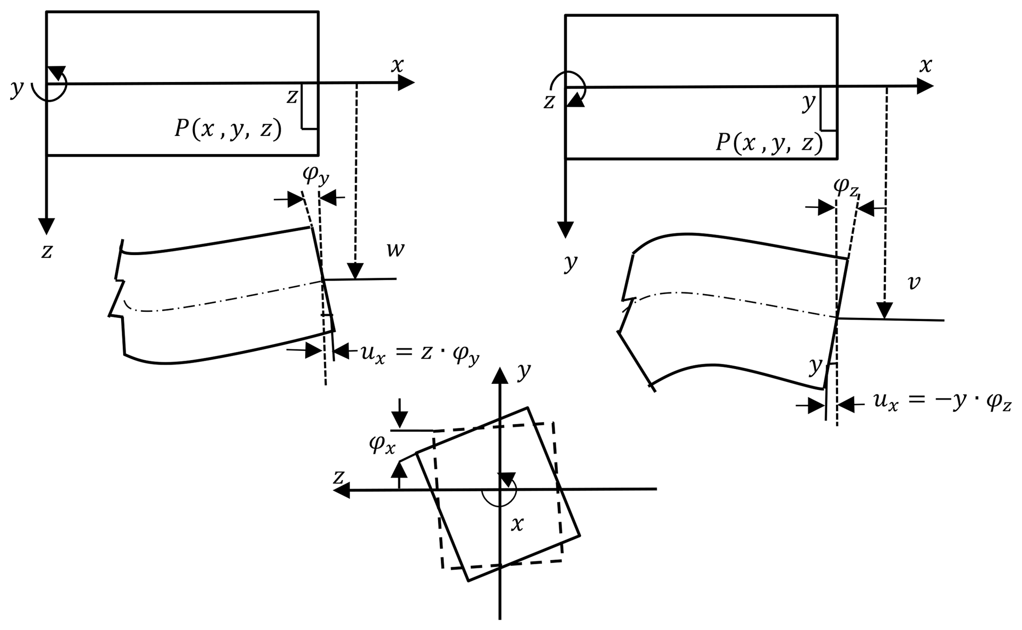
As seen in Fig. 1, the displacement vector up can be expressed at any cross section point P as
The three components of the strains occurring in the beam can be expressed as the derivatives of the displacement functions up, vp and wp. The axial strain εxx and the two shear strain components γxz and γxy are given by the following:
where γz and γy are the constant shear strains that are not neglected in Timoshenko beam theory.
2.2 Principle of virtual work for internal forces
The virtual work components for internal forces corresponding to normal stresses and shear stresses are given by the following:
where N is the axial force, Mz and My are bending internal moments, Qy and Qz are the corresponding shear forces and MTP is the St. Venant torsional moment.
With the introduction of the constitutive relations of Hooke's material law for the stresses corresponding to the internal forces in Eq. (6) and expressing the strains using Eqs. (4a)–(4c) and (5a)–(5b), the virtual work relationship is reformulated as
Here, and are the shear areas in the z and y directions respectively, αsz, αsy are the corresponding shear correction coefficients, A is the cross-sectional area, Ay is the static moment with respect to the z axis, Az is the static moment with respect to the y axis, Ayy is the moment of inertia with respect to the z direction, Azz is the moment of inertia with respect to the y direction, Ayz is the deviation moment of inertia and IT is the torsional moment of inertia.
After the coefficient comparison in Eqs. (6) and (7) the internal forces corresponding to the normal stresses can be expressed by introducing the cross sectional stiffness matrix EA:
The shear stress components in Eqs. (6) and (7) lead to the following relations:
The relation described in Eq. (10a) and (10b) implies that the chosen reference axis coincides with the shear centre due to neglected shear–torsion coupling terms in Eq. (7).
For the special case where the cross section coordinate system coincides with the principal axes, the deformation relationship in Eq. (8) reduces to

2.3 Differential equation system
The virtual work relation in Eq. (7) is rewritten for the case where the beam coordinate system coincides with the principal axis of the cross section – see Eq. (11).
After the partial integration of Eq. (12) the cross section deformation relations and differential equilibrium conditions for the Timoshenko beam element are compiled in a first-order differential equation system (see Eqs. 13, 14). For the Timoshenko beam with an arbitrary beam reference axis at any point on the cross section (see Eq. 8), the system of differential equations can be expressed in the following form:
The differential equation system for the Timoshenko beam with the beam reference axis on principal axes can be represented in the following matrix form:
The entries Sij in Eq. (13) are determined by the inversion of the cross-sectional stiffness matrix in Eq. (8):
In the classical finite element formulation, the beam stiffness matrix and the consistent beam mass matrix are derived by developing an approach for the displacement functions through shape (interpolation) functions, which consist of first- and third-order Hermite polynomials. In this section, an alternative finite element procedure is presented, based on the numerical Runge–Kutta fourth-order integration of the differential motion equations. The integration of the static part (the coefficient matrix in Eqs. 13 and 14 respectively) leads to the static field matrix, while the integration of the inertia terms in the equation of motion Eq. (16) results in a kinetic field matrix. In the last step of the integration, using both field matrices, the respective element stiffness and the element mass matrices can be calculated using simple matrix operations.
3.1 The differential equations of motion
The differential equations of motion for the differential beam element (see Fig. 2) can be written in a matrix form according to Stanoev (2007) and Müller (2012) as follows:
In the above-mentioned equation, matrix A is the coefficient matrix (see Eqs. 13, 14) and vector is the state vector, where
The vector contains the known excitation forces; however, for an eigenvalue problem b=0. The coefficient matrix A and the state vector z in addition to excitation force b constitute the static part of the motion equation. The kinetic part of the motion equation can be expressed using a matrix of the interpolation functions and nodal acceleration vector as follows:
where is the vector of accelerations, [Φ1(x) Φ2(x)]ϵR(6×12) is the matrix of interpolation functions (see Sect. 3.3), is the vector with nodal accelerations and mϵR(6×6) is the inertia matrix of the differential beam element (see Sect. 3.2).
3.2 The inertia matrix term
The inertia matrix in Eq. (18) implies that the distributed mass μ(x) (kg m−1) is applied eccentrically at any location (y,z) in the cross section. The inertia matrix is expressed according to Stanoev (2013):
where Θp, Θy and Θz in (kg m) are the mass moments of inertia for the cross section.
3.3 Shape functions for the Timoshenko beam element
The acceleration term in Eq. (17) is expressed using the product of Hermite interpolating polynomials and the nodal acceleration vectors and .
Shape functions for axial and torsional deformations u(ξ) and φx(ξ), respectively, are derived using first-order polynomial as follows:
To express the coefficients aj in terms of the nodal displacements , or in terms of the torsion the following relations are applied to Eq. (20):
Substituting Eq. (21) into Eq. (20) results in the shape function for axial deformation
and in the following function for torsional deformation φx:
The relationships in Eq. (10a), Eq. (11) and the corresponding part of Eq. (14) are a starting point to derive approximation functions for bending deformation in the xz plane:
Using the above-mentioned relation the expression for w′ is given by
The translational deformation function w(ξ) is approximated by a cubic polynomial function:
Using the constant shear strain relation in Eqs. (5b) and (26) the polynomial expression for constant shear strain can be deduced as follows:
By including Eqs. (27) and (26) in Eq. (25) the polynomial expression for φy(ξ) results in
To determine the coefficients cj the following boundary conditions are applied:
The inversion of Eq. (29) yields
The interpolation functions for and , Eqs. (26) and (28), can be expressed by employing Eq. (30):
where the products of both matrices Nw and Gw are introduced as functions .
In Eq. (32), the functions () are introduced in an analogous manner.
A similar method is used for determining the approximation functions v(ξ) and φz(ξ) for bending deformation in the xy plane.
Starting with Eqs. (10b), (11) and (14), the following is obtained:
The approximations analogous to Eqs. (31) and (32) can be derived as follows:
The H∗j functions developed in Eqs. (31), (32), (35) and (36) are “static” shape functions for the Timoshenko beam. Supposing dependence on time alone for the nodal displacement vectors V(a) and V(b), the matrix of the interpolation functions [Φ1(x) Φ2(x)] in the inertia term Eq. (17) can be developed using Eqs. (31), (32), (35) and (36) (see Kusuma Chandrashekhara, 2018):
3.4 Numerical integration
The special form of the numerical Runge–Kutta fourth-order integration method applied here is described in detail in Müller and Wolf (1975) and Schenk (2012). The integration operator is applied to the equations of motion in Eq. (16), i.e.
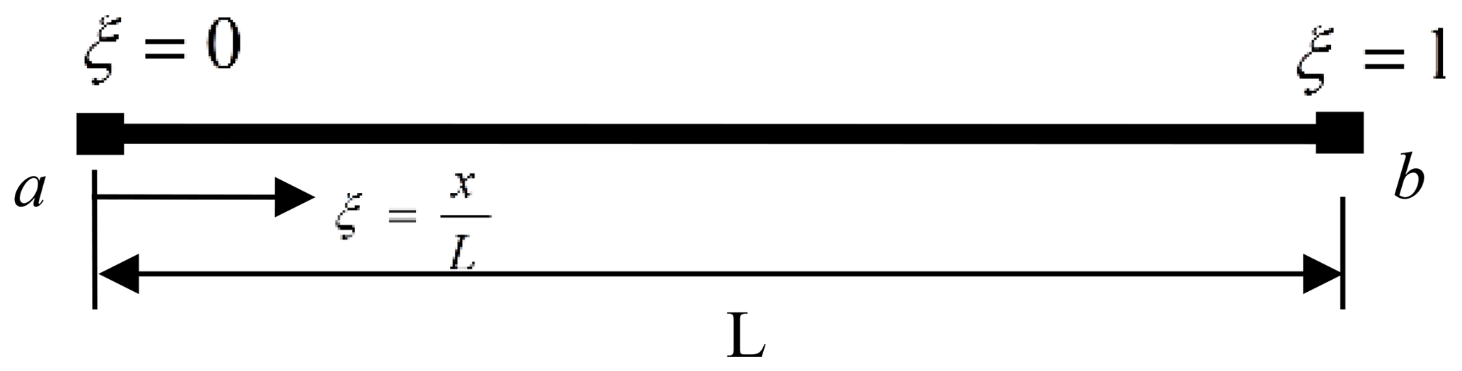
In order to gain sufficient numerical precision the beam axis needs to be divided into at least 20 integration intervals. The integration operator transfers the known state vector at beginning of the integration interval to the end of the interval. The integration procedure starts with the state vector at the first node a, i.e. at location (x=0):
The integration operator is subsequently applied to the evaluated coefficient matrix A at each interval by excluding the initial state vector z(a). The result are static field matrices F(x,a), multiplicatively linked to z(a) see Eq. (40). Therefore, each F(x,a) matrix “transfers” the state vector at location (x=0) to the end x of the integration interval considered (transfer matrix method). In the frame of the integration procedure the actual field matrix F(x,a) serves column wise as an initial vector for the next interval, and the components of the state vector z(a) remain excluded. The beam “load” vector , Eq. (38), evaluated in the actual interval, yields the column in the F(x,a) matrix after integration – Eq. (40).

The numerical integration of the inertia term bm in Eq. (38) is carried out column wise analogously to the “load” vector, by excluding the nodal accelerations – the results are kinetic field matrices H(x,a) at the end of each integration interval (at location x) (see Eq. 40):
This type of numerical integration allows (slightly) varying values of the coefficients of the A matrix, the bm inertia term and the b vector along the beam axis – i.e. all stiffness, mass and external load values of the beam element may vary. After the last integration step at the second node b, at location (x=L), static L(e) and kinetic H(e) field matrices are obtained:
where
According to Eqs. (13) and (14) the state variable z1 represents six-component displacement vectors for V(a) and V(b), respectively, and the state variable z2 represents six-component internal forces vectors S(a) and S(b), at locations (x=0) and (x=L) respectively.
3.5 The element stiffness and mass matrices
By solving the matrix equation in Eq. (41a) for S(a) and S(b), and accounting for the definitions of internal forces in finite element beam formulation (see Fig. 2),
one can derive the element stiffness matrix K(e), the element mass matrix M(e) and the element forces and moments F0 using simple matrix operations as shown in Eq. (43). Then the beam element relationships for the internal forces can be formulated as
3.6 Single masses at eccentric positions
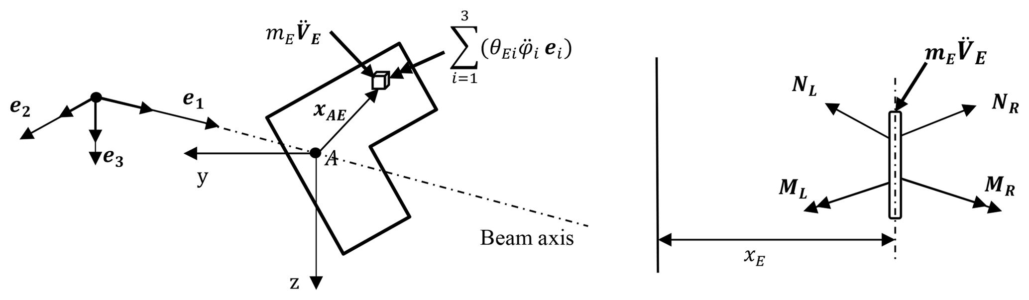
The numerical integration according to Runge–Kutta, described in Sec. 3.4, offers the possibility of including single load or mass quantities within a beam element. Single eccentric masses can be taken into account at the integration interval boundaries. In the local coordinate system of the beam element, at a general position vector , the eccentric mass and the vector representation of dynamic equilibrium, Eq. (44a)–(44b), is as shown in Fig. 4. The beam reference axis is at point A, and vector represents the acceleration vector at the point of application (x,xAE). With the help of the dynamic equilibrium conditions Eq. (44a)–(44b), additional inertia forces and moments due to eccentric mass can be determined (see Li, 2016):
where NL and NR are internal force vectors on the left and right in differential proximity to the point at location x, ML and MR are internal moment vectors on the left and right in differential proximity to the point at location x (see Fig. 4), mE is the eccentric single mass, ΘEi are the mass moments of inertia of the single mass and are the angular accelerations at location x.
The additional inertia matrix , derived from Eq. (44a)–(44b), is analogous to the inertia matrix due to distributed mass in Eq. (18). During the numerical integration within the beam element (see Sect. 3.4) an additional eccentric inertia term has to be added to the kinetic field matrix at the end x (the point of application of eccentric mass) of the corresponding integration interval – see Eqs. (40) and (45).
Single masses do not usually appear in a rotor blade model, but the same finite element may be used for the modelling of wind turbine towers. In this case single masses within a finite beam element could represent bolted ring flange connections or the mass of any equipment, such as lifts etc.
Table 1First three calculated (bolded values) flapwise and edgewise eigenfrequencies.
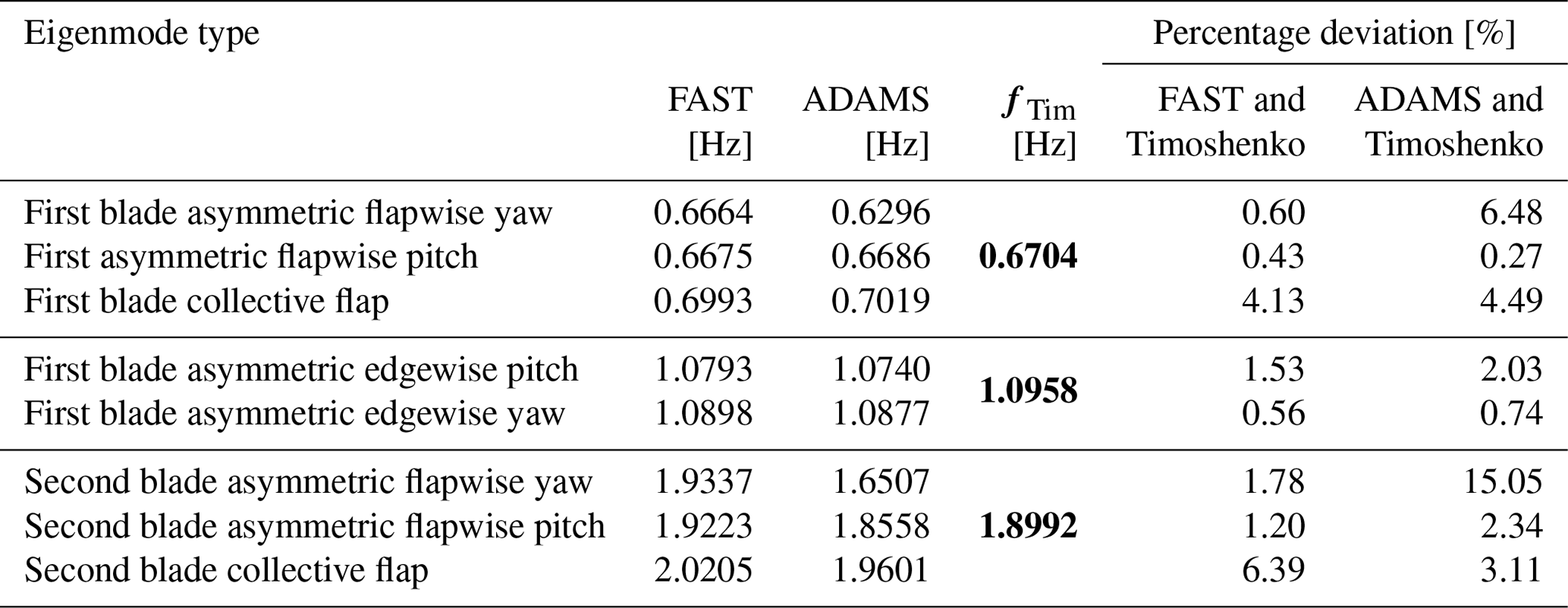
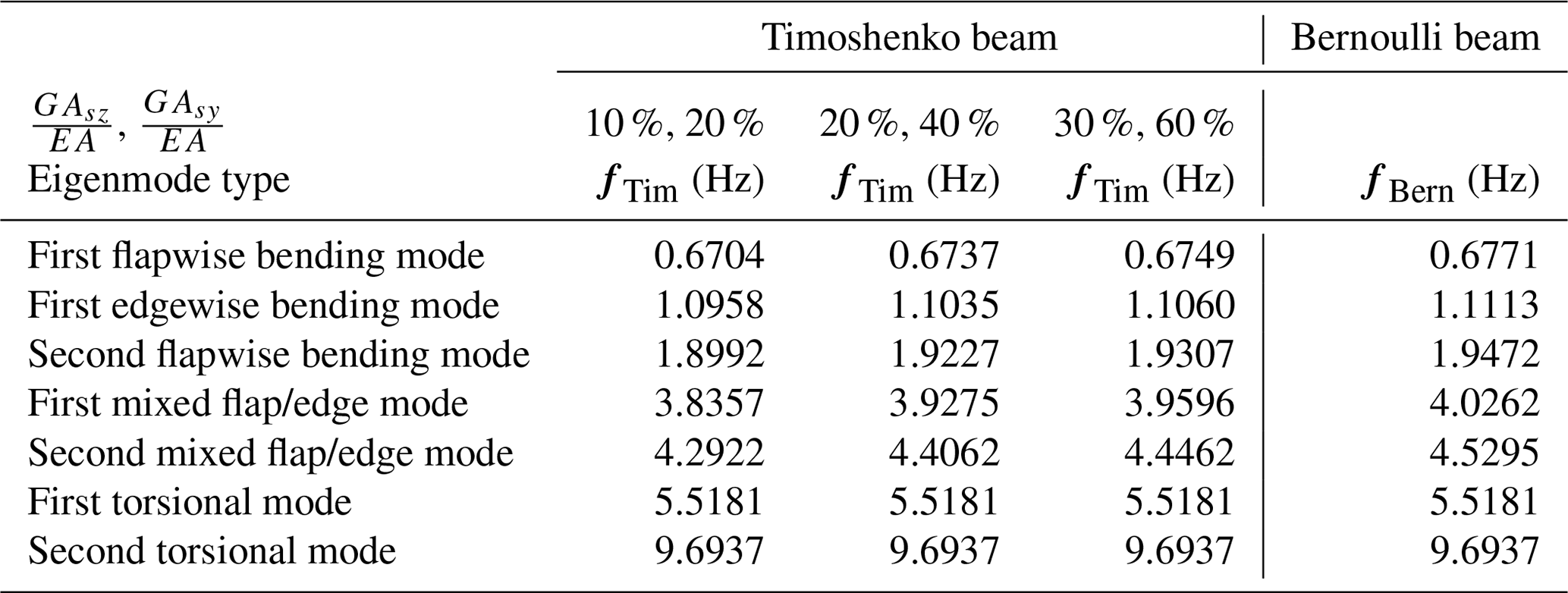
Table 2Comparison between Timoshenko and Bernoulli beams with three variants for shear stiffness values.

The system matrices for a rotor blade beam model are assembled in the usual finite element manner employing the developed element matrices K(e) and M(e) from Eq. (43). In the case of free damped oscillation, the linear homogenous differential equations of motion are given by
where MϵR(n×n) is the system mass matrix, KϵR(n×n) is the system stiffness matrix, DϵR(n×n) is the system damping matrix and q(t)ϵR(n×1) is the nodal displacement vector. The system matrices are symmetric and positively definite for finite element structures. For a free undamped system, the equation of motion is reduced to
By introducing the following solution approach which is given by
into the equation of motion (Eq. 47) the following eigenvalue problem is obtained:
where I is a unity matrix. The condition for non-trivial solution for Eq. (49) is given by
The n-grade characteristic polynomial has n real solutions (eigenfrequencies) and n associated eigenvectors , calculated from Eq. (49). For real-life tasks the solution is usually acquired by use of eigensolver software.
The programming code for the procedure and the graphic plots described/shown below was written in MuPAD, a symbolic math toolbox in MATLAB® (see Kusuma Chandrashekhara, 2018). The code was verified using realistic data for a wind turbine rotor blade. The blade structural data belong to a 5 MW reference wind turbine designed for offshore development (Jonkman et al., 2009). The blade is 63 m in length and is divided into 48 beam elements. The blade structural data consist of distributed mass (mL), blade extensional stiffness (EA), flapwise stiffness (EAzz), edgewise stiffness (EAzz), torsional stiffness (GIT), flapwise mass moment of inertia (Θy) and edgewise mass moment of inertia (Θz). Due to the lack of shear stiffness data in Jonkman et al. (2009), the values of (GAsz) and (GAsy) (used for the calculations in Table 1) – the respective edgewise and flapwise shear stiffness – are estimated to be 10 % and 20 % of extensional stiffness (EA), respectively. The values of the above-mentioned stiffness and mass moment of inertias are specified at spanwise locations along the blade pitch axis and about the principal axes of each cross section as oriented by a twist angle (γ) defined in the input data. The twist angle is incorporated using the rotational transformation of each local element stiffness and mass matrices into the global coordinate system. The results of first three (flapwise and edgewise) eigenfrequencies calculated using the Timoshenko beam model (see Kusuma Chandrashekhara, 2018), are compared with the proposed results from FAST and ADAMS in Jonkman et al. (2009). The results are as shown in Table 1.
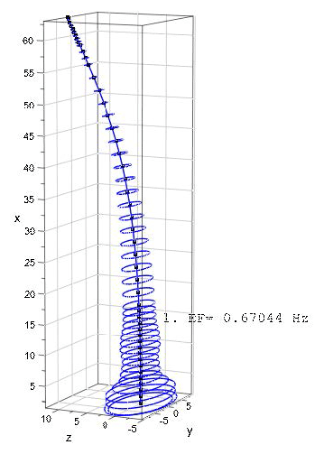
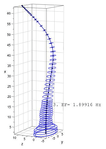
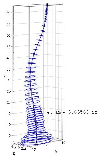
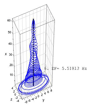
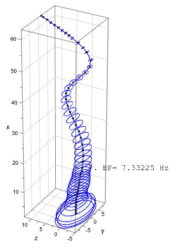
The mode shapes and the corresponding eigenfrequencies for the first flapwise and edgewise eigenmodes as well for two torsional eigenmodes are as shown in Figs. 5–11.
In Table 2 the calculated natural frequencies for three different variants of the shear correction coefficients are shown, approximated as or ratios. The comparison with the frequencies calculated using the Bernoulli beam model outlines the tendency toward a stiffer structure due to the presupposed infinite shear stiffness in this case. Natural frequencies fBern are 0.5 %–1.0 % higher on average than fTim – in the (30 %, 60 %) case. The natural frequencies remain unchanged for both beam models for the purely torsional modes only. The reason for this is that the equations for torsion and bending are uncoupled (for the case of the principal axes, see Eq. 14) and remain the same in both models.
The proposed Timoshenko beam element in the 3-D description has been developed on the basis of the transfer matrix method. Both static and kinetic field matrices for the beam element are derived by applying a Runge–Kutta fourth-order numerical integration procedure on the differential equations of motion in a special way. Appropriate shape functions for the Timoshenko beam have been used to approximate the inertia forces in the motion differential equation. The beam element stiffness and mass matrices are assembled by matrix operations from the derived element field matrices. The usual finite element equations of motion for the rotor blade model are cast in the general case accounting for the structural twist angle and possible pre-bending. Therefore, in the general case the rotor blade beam model represents a polygonal approximated space curve.
For the sake of verification, the natural frequencies and associated eigenmodes are calculated using real-life rotor blade data with the incorporation of realistic twist angle data. The first two edgewise and flapwise eigenfrequencies obtained are compared with the proposed results from FAST and ADAMS software given in Jonkman et al. (2009). It can be observed that the deviation of the results of the Timoshenko beam model from FAST is comparatively lower and is in good agreement with FAST; thus, it can be stated that the approach presented regarding alternative finite element formulation works well.
One key input parameter for the Timoshenko beam model is the shear stiffness. As it was not the main goal of the present work to determine an appropriate shear correction coefficient for realistic rotor blade data, the numerical example was performed with a very rough approximation for GAsz and GAsy. This was done in order to simply demonstrate the performance and the differences to the Bernoulli beam model. However, if detailed data for the complex multilayer design of a rotor blade were available, a more realistic estimation of the shear stiffness could be expected. A workable method for the determination of the shear correction coefficient of a real-life rotor blade represents an important topic for further research.
Data used in this work as rotor blade structural data for the numerical example are publicly available at https://www.nrel.gov/docs/fy09osti/38060.pdf (last access: 25 January 2019; Jonkman et al., 2009). The MATLAB® program code written to calculate the rotor blade is available upon request.
ES led the underlying master thesis (Kusuma Chandrashekhara, 2018) and developed the overall method theoretically by the use of the sources referenced. SKC developed and wrote the code for the Timoshenko shape functions used in the inertia term. He composed the MATLAB® code using different existent code parts and optimized many of the procedures. SKC also performed the calculation and the graphic plots of the numerical example.
The authors declare that they have no conflict of
interest.
Edited by: Lars Pilgaard
Mikkelsen
Reviewed by: two anonymous referees
Andersen, L. and Nielsen, S. R.: Elastic Beams in Three Dimensions, Department of Civil Engineering, Aalborg University, Aalborg, 2008.
Bazoune, A. and Khulief, Y.: Shape Functions of Three-Dimensional Timoshenko Beam Element, J. Sound Vib., 12, 473–480, 2003.
Graf, W. and Vassilev, T.: Einführung in computerorientierte Methoden der Baustatik, Verlag Ernst&Sohn, Berlin, 2006.
Jonkman, J., Butterfield, S., Musial, W., and Scott, G.: Definition of a 5-MW Reference Wind Turbine for Offshore System Development, Technical Report NREL/TP-500-38060, National Renewable Energy Laboratory, Colorado, 2009.
Jureczko, M., Pawlak, M., and Mezyk, A.: Optimisation of wind turbine blades, J. Mater. Process. Tech., 463–471, 2005.
Kaya, M. O.: Free vibration analysis of a rotating Timoshenko beam by differential transform method, Aircr. Eng. Aerosp. Tec., 78, 194–203, 2006.
Kusuma Chandrashekhara, S.: Calculation of natural vibrations of wind turbine rotor blades using Timoshenko beam elements in the frame of MATLAB, Master Thesis, Chair of Wind Energy Technology, University of Rostock, Rostock, 2018.
Li, N.: Berechnung der 3D-Eigenschwingungen des Rotorblatts einer WEA durch FE-Balkenmodelle mit Hilfe von MATLAB, Masterarbeit, Stiftungslehrstuhl für Windenergietechnik, Universität Rostock, 2016.
Manwell, J., McGowan, J., and Rogers, A.: Wind Energy Explained, Theory, Design and Application, Wiley, West Sussex, 2009.
Müller, H. and Wolf, C.: Stabtragwerke (STATRA) Berechnung des Schnittkraft- und Verschiebungszustandes ebener Stabtragwerke nach Theorie I. und II. Ordnung sowie Stabilitätsuntersuchung, Baustein 1 des Programmsystems STATRA, Grundlagen, Bauakademie der DDR, Verlag Bauinformation, Berlin, 1975.
Müller, K.: Untersuchungen zur Abschätzung von 3D-Schiffskörpereigenschwingungen durch Einsatz effizienter FE-Balkenmodelle mit Hilfe von MATLAB, Diplomarbeit, Lehrstuhl für Schiffstechnische Konstruktionen, Universität Rostock, Rostock, 2012.
Schenk, S.: Entwicklung eines MATLAB-Programmtools zur effizienten Berechnung von Schiffskörpereigenschwingungen durch ein FE-Balkenmodell, Masterarbeit, Lehrstuhl für Schiffstechnische Konstruktionen, Universität Rostock, Rostock, 2012.
Stanoev, E.: Eine alternative FE-Formulierung der kinetischen Effekte beim räumlich belasteten Stab, Rostocker Berichte aus dem Institut für Bauingenieurwesen, Heft 17, Universität Rostock, Institut für Bauingenieurwesen, Rostock, 2007.
Stanoev, E.: Vorlesungsskript: Berechnung dünnwandiger Stabsysteme, Lehrstuhl für Schiffstechnische Konstruktionen, Universität Rostock, Rostock, 2013.
Wu, J.-S.: Analytical and Numerical Methods for Vibration Analyses, Wiley, Singapore, 2013.