the Creative Commons Attribution 4.0 License.
the Creative Commons Attribution 4.0 License.
 | 02 Jan 2020
Implementation of the blade element momentum model on a polar grid and its aeroelastic load impact
Torben Juul Larsen
Georg Raimund Pirrung
Frederik Zahle
We show that the upscaling of wind turbines from rotor diameters of 15–20 m to presently large rotors of 150–200 m has changed the requirements for the aerodynamic blade element momentum (BEM) models in the aeroelastic codes. This is because the typical scales in the inflow turbulence are now comparable with the rotor diameter of the large turbines. Therefore, the spectrum of the incoming turbulence relative to the rotating blade has increased energy content on 1P, 2P, …, nP, and the annular mean induction approach in a classical BEM implementation might no longer be a good approximation for large rotors. We present a complete BEM implementation on a polar grid that models the induction response to the considerable 1P, 2P, …, nP inflow variations, including models for yawed inflow, dynamic inflow and radial induction. At each time step, in an aeroelastic simulation, the induction derived from a local BEM approach is updated at all the stationary grid points covering the swept area so the model can be characterized as an engineering actuator disk (AD) solution. The induction at each grid point varies slowly in time due to the dynamic inflow filter but the rotating blade now samples the induction field; as a result, the induction seen from the blade is highly unsteady and has a spectrum with distinct 1P, 2P, …, nP peaks. The load impact mechanism from this unsteady induction is analyzed and it is found that the load impact strongly depends on the turbine design and operating conditions. For operation at low to medium thrust coefficients (conventional turbines at above rated wind speed or low induction turbines in the whole operating range), it is found that the grid BEM gives typically 8 %–10 % lower 1 Hz blade root flapwise fatigue loads than the classical annular mean BEM approach. At high thrust coefficients that can occur at low wind speeds, the grid BEM can give slightly increased fatigue loads. In the paper, the implementation of the grid-based BEM is described in detail, and finally several validation cases are presented. Comparisons with blade loads from full rotor CFD, wind tunnel experiments and a field experiment show that the model can predict the aerodynamic forces in half-wake, yawed flow, dynamic inflow and turbulent inflow conditions.
Please read the corrigendum first before continuing.
-
Notice on corrigendum
The requested paper has a corresponding corrigendum published. Please read the corrigendum first before downloading the article.
-
Article
(8925 KB)
-
The requested paper has a corresponding corrigendum published. Please read the corrigendum first before downloading the article.
- Article
(8925 KB) - Full-text XML
- Corrigendum
- BibTeX
- EndNote


The blade element momentum (BEM) model (Glauert, 1935) is used extensively within the wind energy research community as well as by the wind turbine industry for simulating the aerodynamic rotor characteristics such as blade aerodynamic loads, rotor power and rotor thrust. For rotor design, the computations are commonly carried out for uniform, constant inflow over the rotor disk. However, the BEM model is also the aerodynamic engine in most aeroelastic models used today (FLEX5 (Flex4), Øye, 1996; FAST, Jonkman et al., 2016; BLADED, Bossanyi, 2003; GAST, Riziotis and Voustinas, 1997; Cp-Lambda, Botasso and Croce, 2006–2013; FOCUS, WMC, 2019; HAWC2, Larsen and Hansen, 2007) by the industry for the detailed aeroelastic simulations that are the basis for the certification of wind turbines (Hansen et al., 2015; IEC, 2005). This comprises a significant amount of simulations at normal operating conditions with turbulent inflow but also at fault modes of the turbines such as a large yaw error. It further includes extreme inflow conditions such as strong shear, gusts and more recently also wake situations, where the wake is modeled as a combination of a reduced, meandering wind speed deficit in the wake region and added wake turbulence (Larsen et al., 2008; Madsen et al., 2010c).
When describing an aeroelastic code, it is often just mentioned that BEM is the model for computing the aerodynamic forces and that the model is further extended with submodels for tip loss, yawed conditions, dynamic inflow and dynamic stall. This is an incomplete description, as implementation details such as the way the models are coupled together can influence the computational results considerably. The most important aspect is how the BEM model is implemented to model the induction response due to the unsteady and non-uniform loading over the rotor caused by the atmospheric turbulent inflow, wind shear or control actions like pitch and flap control.
The purpose of the present article is to present in detail a complete unsteady BEM induction model for non-uniform inflow and loading that can be readily implemented.
1.1 Upscaling has influenced the requirements for aerodynamic modeling
The non-uniform unsteady loading over the rotor disk due to the atmospheric inflow increases with rotor size. Thus, the requirements to the BEM modeling capability have changed considerably from the 15–20 m diameter rotors in the 1980s to 100–200 m rotors today. This important effect of turbulence scales relative to rotor size was already described by de Vries (1979), noticing the difference in impact on aerodynamic loads of turbulence scales above and below the rotor size. de Vries (1979) also very briefly presented how to use the BEM method in sheared inflow. This approach has some resemblance to the BEM implementation that will be presented here.
To illustrate how the upscaling of rotors leads to a more non-uniform inflow and thus non-uniform loading of the rotor when operating in turbulent inflow (no shear), we simulate two turbines with the aeroelastic code HAWC2 (Horizontal Axis Wind turbine simulation Code; Larsen and Hansen, 2007): the AVATAR rotor with a diameter of 205 m (Sieros et al., 2015) and a downscaled version of the AVATAR rotor with a diameter of 51.4 m. Both turbines were simulated without tilt, with a stiff structure, and both operate at the same tip speed of 74.7 m s−1 and in the same turbulent inflow with no shear. The turbulent inflow was generated with the Mann model (Mann, 1994) using a box with vertical and horizontal side lengths of 240 and 5600 m, the latter corresponding to the traveling length of the turbulence over the simulation time of 700 s and a mean wind speed of 8 m s−1.
As the turbine blades rotate through the turbulent vortex structures, the spectrum of the free wind speed at the tip of the blades has energy concentrated on multiples of the rotational frequency 1P (Fig. 1). Since the size of the turbulent vortex structures is absolute (given a certain turbulence length scale), the distribution of energy upon the individual frequency multiples is different for different turbine sizes. What can be noticed is that the small rotor has a significant amount of energy on the very low frequencies (≪1P), whereas the larger turbine experiences a higher ratio of the total energy on 1P and multiples. In other words, for the increasing size of turbines, a bigger and bigger part of the turbulent eddies have a size comparable to or below the rotor diameter.
The increasingly non-uniform rotor loading with turbine size is also caused by inflow with shear. The largest modern turbines with the blade tips at top positions around heights of 300 m now span most of atmospheric boundary layer containing the main part of the shear (Pena Diaz et al., 2009). This is in particular seen for stable flow situations.
Other challenging wind situations comprise non-stationary wind conditions containing trends, such as wind shear developing over time. For very large rotors, these situations are important for the extreme load levels during operation. Thus, they need attention in the modeling phase if turbine designers shall be able to counteract such events using either active or passive load alleviation techniques.
Besides the upscaling trend, turbine design has changed in the same time span of years, which results in new requirements for the aerodynamic modeling in the aeroelastic codes. Pitch control is now the common power regulation method; therefore, situations like pitch fault have to be simulated for certification. Such a situation with, e.g., one blade pitch differing from the pitch of the other blades with, e.g., 20∘, results in a non-uniform rotor loading and expected azimuthal variation of induction. The pitch control for power regulation has been extended to include cyclic pitch to alleviate 1P loads, and now full individual pitch is being implemented for even better load alleviation. An important question is thus how to handle individual pitch action in a BEM-type modeling.
1.2 Research on the challenges in modeling sheared and turbulent inflow
The subject of sheared and turbulent inflow was part of the work in the EU-funded UpWind project (2006–2011) with the main objective to study upscaling of turbines to 8–10 MW. The aerodynamic flow mechanisms at high shear in the inflow were investigated by simulating the sheared inflow on the 5 MW reference wind turbine (Jonkman et al., 2009) with a range of models from high-fidelity CFD codes to vortex codes and to more BEM-type codes (Madsen et al., 2012). One major finding was that all high-fidelity codes and vortex codes showed that the induction does vary within an annular element for sheared inflow. Different BEM implementations to cope with this were discussed.
Similar work was continued in the EU-funded AVATAR project (2013–2017) with a focus on even bigger turbines (10 MW and higher) than in the UpWind project. A summary of the findings has been presented by Schepers et al. (2018a). One major finding was that a comparison of aeroelastic simulations with a free vortex code and a BEM-based aeroelastic code showed an overprediction of fatigue loads in the range of 15 % by the BEM-based aeroelastic code. It is further mentioned and discussed that the results depend on the actual implementation of the BEM model.
1.3 The historical BEM development
The basic BEM formulation originates from Glauert and was developed for airplane propellers (Glauert, 1935). Glauert points out that the two major components are the “momentum theory” and the “blade element theory” which for many years were developed separately and, e.g., the use of finite aspect blade data was considered in the blade element theories to fit experimental rotor data. However, the combination of the two theories finally led to the BEM approach where the induced velocities at the rotor disk are derived from the momentum theory and the blade sectional forces are found on the basis of infinite aspect ratio (2-D) airfoil characteristics. In the present paper, the focus is on the momentum part of the BEM approach, although many uncertainties in rotor computations are linked to the blade element analysis such as 3-D airfoil characteristics due to rotational effects.
When the momentum part of the BEM theory is used in aeroelastic simulations, the actual flow conditions violate most assumptions in the basic theory: (1) turbulent and sheared inflow compared with the assumption of uniform, steady inflow; (2) non-uniform load in contrast to the assumed uniform loading and (3) skewed inflow in contrast to assumed axial inflow, just to mention the most important violations. To compensate for this, a number of submodels are introduced like dynamic inflow and skewed wake models. However, there is no real consensus on how the different phenomena should be modeled and how the submodels should interact. Therefore, we often see considerable deviations for BEM simulations on complex inflow cases (Hand et al., 2001; Schepers et al., 2018b).
Many researchers have contributed over time to the development of the BEM theory for wind turbines but only a few will be mentioned here. Wilson and Lissaman (1974) made an important contribution at an early stage to describe the theory. They also proposed a method based on a Taylor expansion to look into the effect of wind shear. Another important contribution at an early stage to the development of the BEM approach is made by de Vries (1979), who envisioned the challenges in implementing the BEM theory for turbulent inflow.
Later, a comprehensive description of the BEM modeling is presented in the handbook of Burton et al. (2011) with a detailed discussion of inflow models to handle dynamic and skewed loading as will be discussed later. Also, the handbook of Hansen (2015) gives a fundamental introduction to the BEM modeling approach as well as the doctoral thesis by Sørensen (2016).
1.4 The organization of the paper
In Sect. 3, we present a detailed description of the implementation of the grid BEM approach. However, first, in that section, we give a short introduction to the origin of the CFD simulations of the actuator disk flow used heavily in developing and tuning the submodel for yawed flow, the dynamic induction model and a submodel for radial induction. The mechanism of induction in turbulent and sheared flow is explored in Sect. 4, and we present the load and power impact for two turbines for design load case (DLC) 1.2 load cases. In Sect. 5, a selection of validation cases is presented, followed by conclusions in Sect. 6.
The overall idea with the present BEM implementation is to model the rotor as an actuator disk (AD) that is updated at each time step in stationary grid points covering the rotor disk. In an aeroelastic simulation, the loading will normally be non-uniform and unsteady as discussed above. The input to the computation of the induced velocities is thus the distributed normal and tangential loading on the AD, and it will be shown in Sect. 2.4 how the loading of the individual rotor blades is distributed over the disk. The flow field could be computed with a CFD model of the AD (Madsen, 1999), but we present here an engineering solution based on the BEM theory for the flow at the disk to reduce the computational efforts to a minimum. However, the close link between the engineering BEM-AD and the AD-CFD model means that we easily can tune submodels in the BEM-AD model. We use AD-CFD results below for tuning the yaw and dynamic inflow model and for correction of the momentum model at high loading. Another example of such submodel tuning is the correction for the influence of wake rotation and expansion (Sharpe, 2004), as presented by Madsen et al. (2010a). However, these submodels are not incorporated in the BEM-AD model presented here. Before going to the description of the BEM model, we will briefly introduce the origin of the AD-CFD results used below.
2.1 The basis of the AD-CFD results
The general purpose CFD code FIDAP (Fluid Dynamics Analysis Program), based on the finite element method, is used for the AD computations. It was one of the first commercially available CFD codes and has an unstructured mesh capability which reduces the requirements to the total number of nodes.
In the past, the code has been used for several studies of the flow through an actuator disk model. In a first setup from 1996, the computations show good correlation with the momentum theory with one-third induction at the rotor disk and two-thirds in the far field for a prescribed uniform loading corresponding to a thrust coefficient of 0.89 (Madsen, 1997). It should be mentioned that FIDAP has an option of using a discrete pressure formulation from element to element which was found important for AD simulations of the pressure jump at the disk. Typically, two cells with a total axial distance of 0.05R are used to model the disk in axial direction.
Later, in 1999, the AD model was coupled to the aeroelastic code HAWC (Thirstrup Petersen, 1996), so that the computation of the induction could be shifted between BEM and the CFD-AD model (Madsen, 1999). Several yawed flow cases for a 100 kW turbine were investigated with that model setup and a good correlation with experimental data was found, e.g., for the electrical power and flapwise moment (Madsen, 2000). A further comparison was made using the data set for 45∘ yaw error from the NREL phase VI 10 m wind turbine tested in the NASA Ames 80 ft × 120 ft wind tunnel (Hand et al., 2001). The computed angle of attack variation at a radial position of 83 % showed good correlation with the measured inflow angle when corrected for the influence of upwash.
The CFD mesh and model from this setup is used for the present simulations with a prescribed uniform loading on the disk (Fig. 2). The mesh extends 10 rotor diameters (D) in the z direction, which is the main flow direction for zero yaw, 12D in the x direction and 4D in the y direction. The inflow plane is 4D upstream the actuator disk, and yawed flow is simulated by changing the inflow direction with an x-velocity component. In total, about 25 000 nodes are used for the meshing.
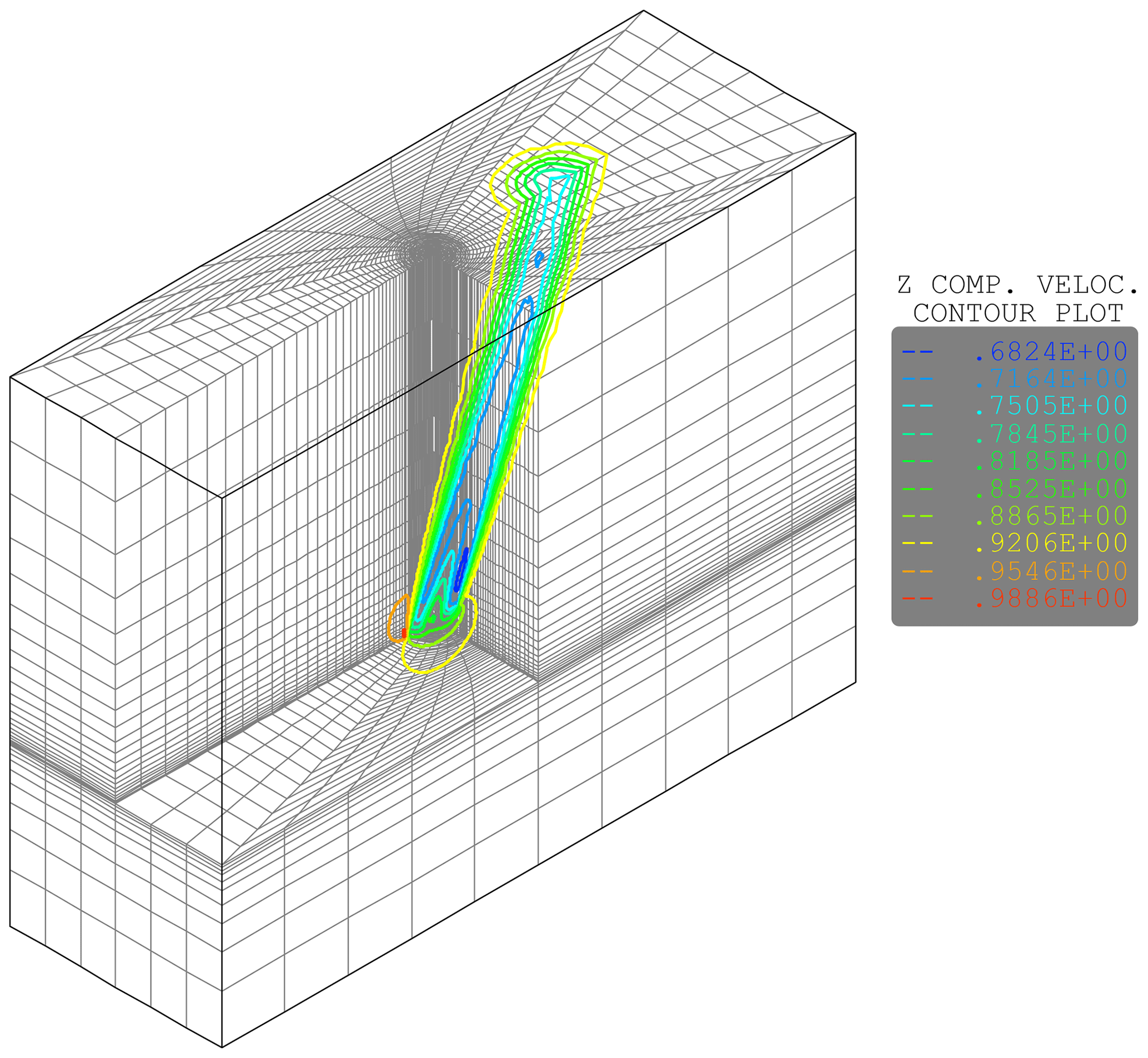
Figure 2The CFD mesh used for the AD yaw computations. The velocity contours for computation of a 30∘ yawed case are shown on top of the mesh plot.
2.2 The basic BEM equations
The fundamental part of the BEM model (Glauert, 1935) is the relation between thrust on the rotor and the induced velocities. For a stream tube enclosing the AD, a 1-D momentum balance between axial forces on the turbine and the flow within a stream tube is . Following classical literature like Glauert (1935), Wilson and Lissaman (1974) and de Vries (1979), this leads to the relationship between the thrust coefficient CT and the induction factor a:
where and with the rotor thrust T, the free-stream velocity U0, the air density ρ and the rotor area A.
For thrust values causing higher induced velocities than a=0.5, Eq. (1) breaks down, since the flow velocity in the wake far downstream according to the momentum theory is 1−2a, which in these cases is equal to or smaller than zero. This results in an infinite expansion of the flow behind the rotor and the flow can no longer be approximated by simple momentum theory. More complex flow models are needed, such as CFD, or an empirically based relation can be used.
For different reasons explained below, we use a BEM implementation where the induction in the whole operational range from negative CT to a high positive CT is expressed through the following third-order polynomial shown in Fig. 3:
where the coefficients k1 … k3 are defined as k1=0.2460, k2=0.0586 and k3=0.0883.
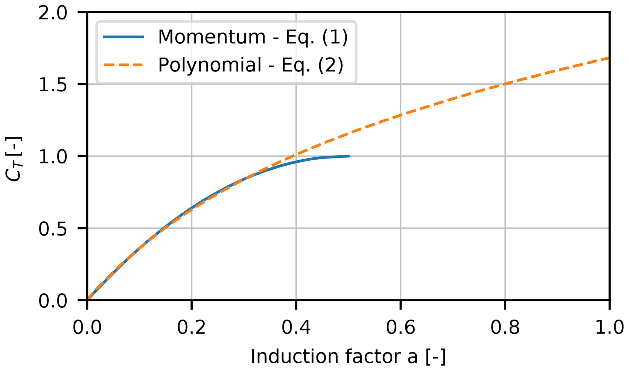
Figure 3The approximation of the basic momentum relation between CT and a with a polynomial extending into an empirical relation at high loading when CT is above 0.89.
For CT<0.89, the polynomial fits well the momentum equation. At high loading, the curve was determined to fall between the Glauert empirical relation fitted to experimental results for a model rotor (see, e.g., Burton et al., 2011) and results from actuator disk simulations at high loading (Madsen, 1997). At high values of CT>2.5, the gradient of the a(CT) curve is kept constant. Thus, a is determined as .
One important reason for using a polynomial fit to Eq. (1) is that we find that it is a more robust and fast method to compute the induction instead of solving Eq. (1) using a non-linear Newton–Raphson iteration solver combined with an empirical relation at high loading. Another reason is that it makes it easily possible to modify this CT(a) relation in order to simulate, e.g., a coned rotor as illustrated in Madsen et al. (2010a), using AD-CFD simulations for the coned rotor. In this case, the CT(a) polynomials will be a function of radial position.
A next step in implementing the BEM model is to couple the momentum theory to the blade element theory where the forces on a blade section are derived by means of two-dimensional airfoil characteristics. We apply Eq. (1) on a ring element of the rotor with the radial extension dr, as illustrated in Fig. 4a:
where Urel is the relative velocity to the blade section, c is the blade chord, NB is the number of blades, and Cy is the projection of the lift coefficient Cl and the drag coefficient Cd on a line perpendicular to the rotor plane.

Figure 4Illustration of the BEM approach. (a) Classic approach using an annular element to which the load is assumed constant over the element (mean value of blade forces). (b) New induction grid with annular elements and further subdivided azimuthally.
Besides the elemental thrust dT on the ring element, there is also a torque dQ, and we can define a torque coefficient CQ by
where Cx is the projection of the lift coefficient Cl and the drag coefficient Cd on a line tangential to the rotor plane.
Applying the angular momentum equation across the disk, we get
Combining Eqs. (4) and (5), we find
where a′ is the tangential induction coefficient. To avoid division by zero, the 1−a term is limited to a minimum of 0.1 for a>0.9.
2.3 Tip correction
The relation between thrust and induced velocities (Eqs. 1–2) is changed due to the presence of tip effects, caused by a finite number of blades. Within the wind turbine research community, the tip correction method has for a long time been the subject of numerous investigations and development. In a recent work, Sørensen (2016) presents a comprehensive review of studies on the tip correction and contributes with full derivation of the commonly used Prandtl tip correction which, however, was further slightly modified by Glauert (1935) to be used in the BEM theory. The Prandtl tip correction factor F is presented by Glauert (1935):
We insert it into the momentum equation (Eq. 1) as
where has to be inserted instead of CT in Eq. (2). The term can reach very large values close to the tip where F becomes very small. In the code, the term is limited to a maximum value of 4. How to incorporate the tip correction factor is also discussed by Sørensen (2016), concluding that it can either be used to modify the circulation (loading) as done here or through a modification of the induced velocities.
2.4 Specific grid BEM implementation in HAWC2
Even though the BEM relationship is originally derived for a full rotor, it is generally implemented on an annular element form as proposed by Glauert (1935). In such an annular BEM implementation, it is assumed that the loading and induction within each annular element are constant and that the annular elements are independent of each other. The CT coefficient now represents the average axial loading of the blades on an annular ring element.
In order to model azimuthal variations of induction due to azimuthal variations of blade loading as discussed above, we propose to expand the annular BEM approach. Dividing the annular elements into azimuthal sub-elements leads to a polar grid BEM approach; see Fig. 4b.
The induced velocity is found in each grid point using the a(CT) relationship in Eq. (2). For a uniform inflow and loading, this leads to the exact same induction as the classic annular element approach, whereas differences are seen for non-uniform wind loading over the rotor. An important part of this azimuthal annular element approach is the definition of the local induction factor, where the local instantaneous induced velocity at a point in the grid is normalized with the local free wind speed (the wind speed without rotor induction) at the exact same point.
As seen in Fig. 4, a question arises about how to find the local load in grid points that are not at the location of a blade. For the classic annular element, the blade loads are averaged and the resulting blade load is assumed to be constant over the annular element. The solution for the azimuthally divided annular element (grid point) is to compute two different thrust coefficients and torque coefficients. These coefficients use the pitch and velocities of the two neighboring blades combined with the local wind speed and induction at the grid point. The coefficients will be weighted by the azimuthal distance of the respective blades. For the corresponding radial position on these two blades, the transformation matrix from sectional to global coordinates is rotated by the azimuthal distance between the blade and the grid point. This corresponds to virtually rotating the blade position to the position of the grid point. The blade velocities are rotated as well such that, for example, the velocity in the direction of rotation at the blade location is applied as a velocity in the direction of rotation at the grid point. Then, the flow at the grid point can be computed as the sum of the free wind speed , the induced velocity and the rotated velocity of the blade section ; the latter has a negative sign because the flow will be experienced in the opposite direction of the blade movement.
The superscripts “S” and “G” denote sectional and global coordinates, and the subscript b=1, 2 denotes the two closest blades. The angle of attack αb is computed by
and the relative velocity Ur by
and the local thrust in the grid points are calculated as
where Cy(α) is the lift and drag coefficient projected into the axial direction.
The computation of the local torque is done in the same manner. Then, the two resulting thrust and torque coefficients are interpolated based on the azimuth angle Ψ of the two blades b=1, 2 and the azimuth angle of the grid point:
2.5 Yaw modeling
It is evident that skewed inflow to the disk violates the conditions for the basic momentum equation (Eq. 1) so that the momentum considerations used for derivation of the model are no longer valid. When the rotor operates in yaw, there are two main effects on the induced velocities, as described by Glauert (1935). One effect is the change in the mean level of the induced velocities and the other effect is an azimuth variation of the induced velocities, as the wake vortex system is relatively closer to the rotor on one side compared to the other side.
A comprehensive investigation of yaw and dynamic inflow models for wind turbines and dynamic inflow modeling was carried out in the EU-funded project “Joint Investigation of Dynamic Inflow Effects and Implementation of an Engineering Method” (Schepers and Snel, 1995). Here, also a short summary of yaw models for helicopters is presented, as these classical yaw models have been the basis for yaw models for wind turbines. The derivation and tuning of the present yaw model deviates slightly in the way that AD simulations of a uniformly loaded disk are used where cylindrical vortex models were a main source in the project (Schepers and Snel, 1995). However, as the AD and vortex models should give almost the same results, we will see that the present yaw model is close to some of the models from the abovementioned dynamic inflow EU project.

Figure 5(a) Figure showing the reduction factor of the induction a as function of CT for different yaw angles. The solid lines show the analytical value and the dashed lines show the polynomial fit (Eq. 18). (b) Relation between the thrust coefficient CT and the induced wind speed factor a in yawed inflow. The solid lines show the analytical value (Eq. 16), and the dashed lines show the polynomial fit (Eq. 17). The error of the polynomial fit in panel (b) is smaller than 3 % for all shown yaw angles up to a CT of 0.87. For higher CT, the deviations increase, especially for yaw angles above 45∘.
2.5.1 Mean induction in yawed inflow
The general equation relating the thrust and induction at a rotor operating in yaw (see Fig. 6), as proposed by Glauert (1935), is
The equation has not been proven but is generally accepted as a good assumption and commonly used in helicopter AD modeling (Stepniewski and Keys, 1984). Now, the following equation relating the thrust coefficient to the induction can be derived:
where Φ is the yaw angle.
Based on these results, a reduction factor ka for the induction a as function of CT (Eq. 2) for different yaw angles can be derived:
This reduction factor is approximated by a polynomial fit of the form
as shown in Fig. 5a. The values of Ct,mean used in Eq. (18) have to be limited to a maximum value of 0.9 to avoid a bending over of the CT(a) curve. The resulting approximation of the CT(a) curve is compared to Eq. (16) in Fig. 5b. The agreement becomes very good for low loading (CT<0.9) but becomes worse for higher loading. At higher loading, however, Eq. (16) might no longer be valid, which justifies the limiter in Eq. (18).
The parameters ka,i of Eq. (18) are approximated as function of the yaw angle:
The values ki,j are collected in the matrix k:
The wake skew angle χ is found as the default based on the average wake angle using vectors and representing the average local wind speed and induction over the whole rotor; see also Fig. 6.
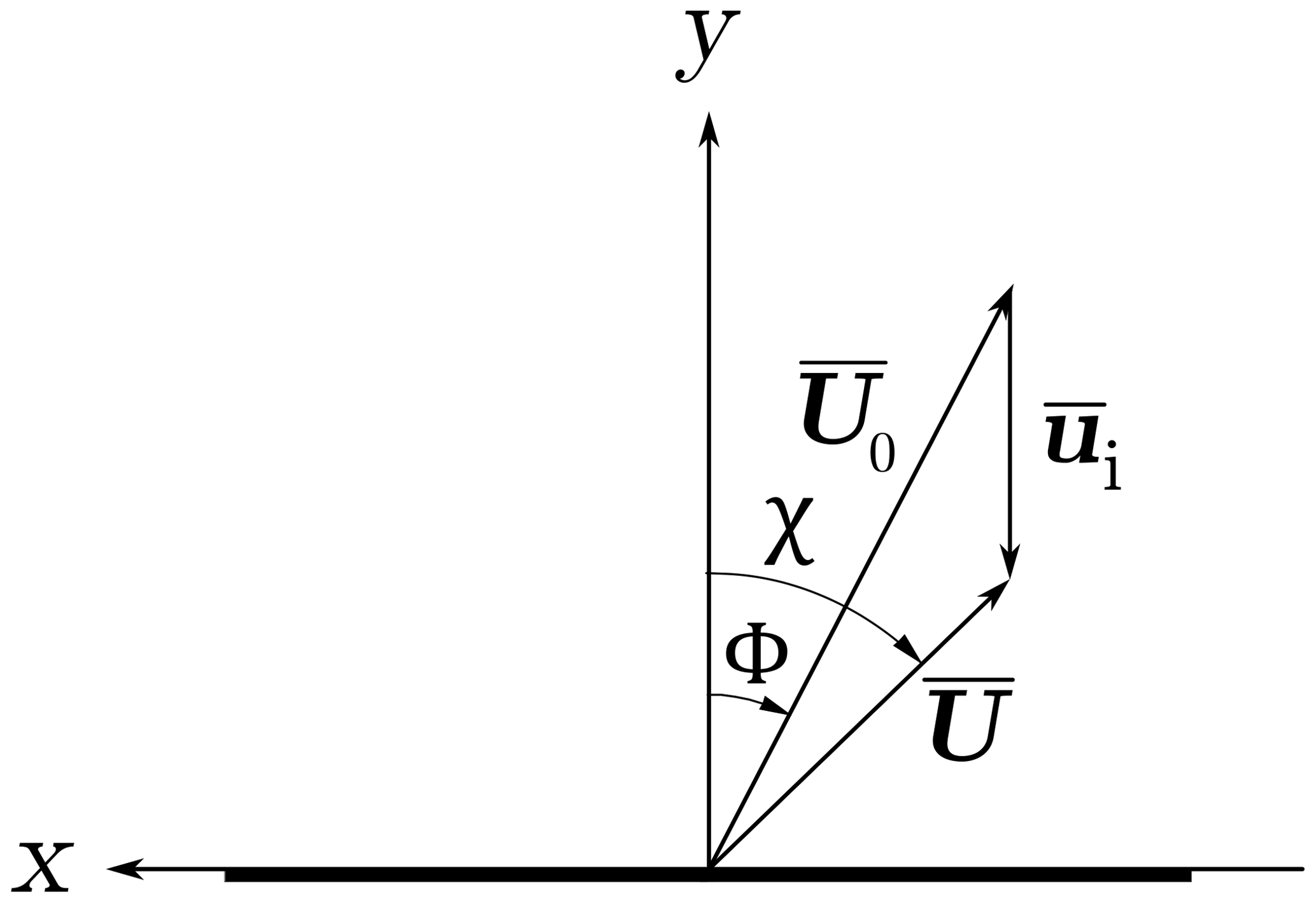
Figure 6Top view of the velocity vectors and angles used for the skew wake expression. The y direction is the default wind direction without any skew inflow.
The wake skew angle χ depends on the thrust coefficient, which is illustrated in Fig. 7. At low loading, χ is close to the yaw angle, but for high loading, it is seen that the wake can be deflected more than 10∘ from the mean wind direction.
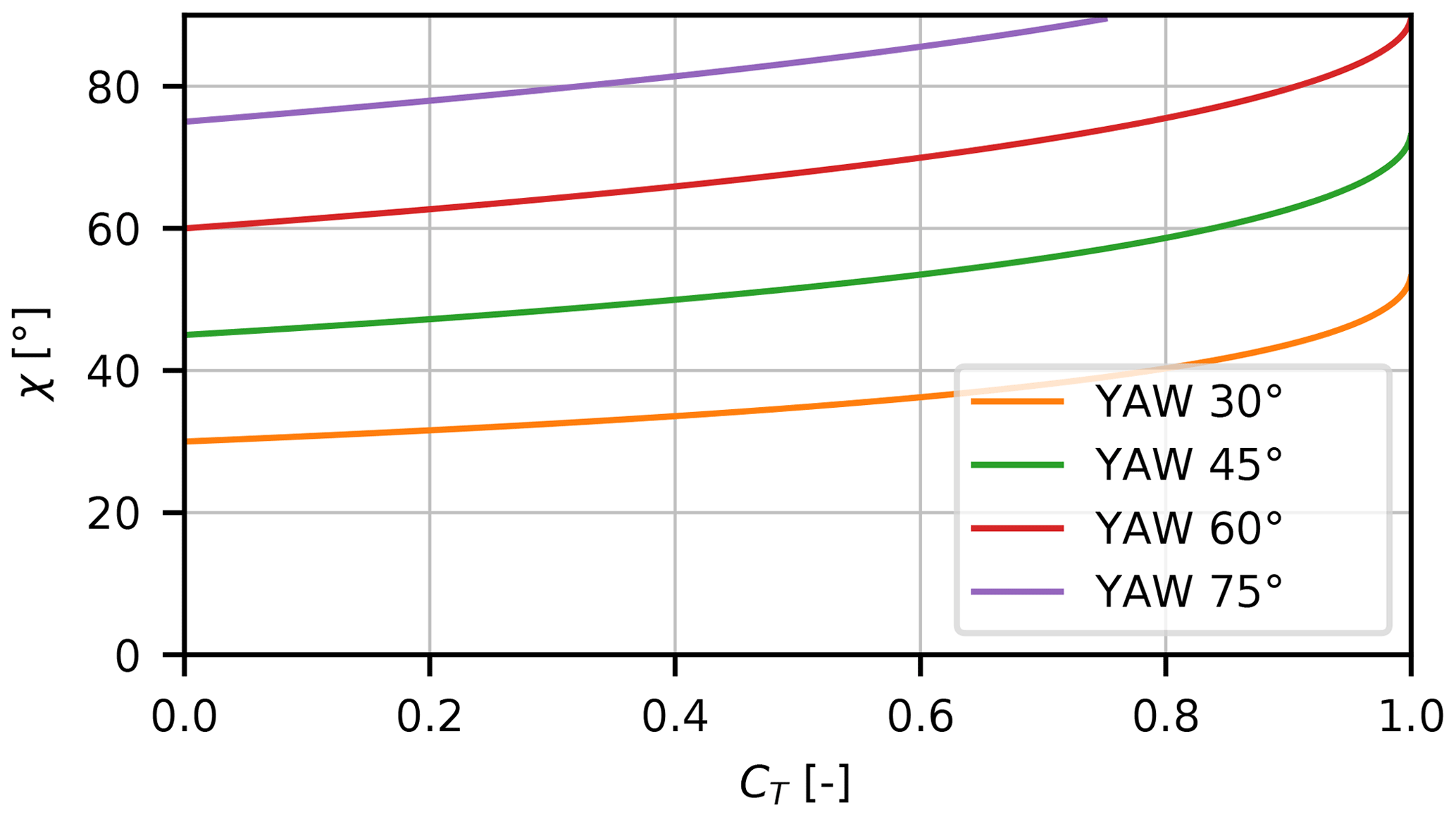
Figure 7The wake skew deflection angle χ against the thrust coefficient for different yaw angles. For zero loading, the angle is equal to the yaw angle, whereas the deflection angle increases in combination with an increased thrust level on the turbine.

Figure 8Comparison of axial velocity through a vertical line (z axis in Fig. 6) through the rotor disk. The rotor loading is prescribed to a constant loading of CT=0.8.
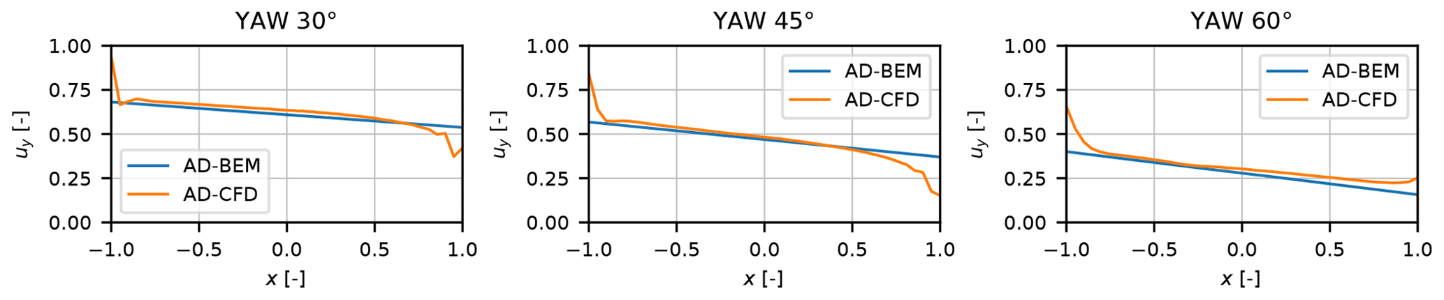
Figure 9Comparison of axial velocity through a horizontal line through the rotor disk. The rotor loading is prescribed to a constant loading of CT=0.8.
2.5.2 Azimuthal variations of induction in yawed inflow
As the wake in the yawed conditions is skewed behind the rotor disk expressed by the skew angle χ (see Fig. 6), the induction will be higher on the side of the rotor towards which the wake deflects. This is because the wake vortices are closer to the rotor on that side.
A very general equation for the azimuthal variation of the induction was presented by Schepers and Snel (1995), containing a Fourier expansion in azimuth angle of the induced velocity at each radial position. Here, we use a slightly simpler expression by Leishman (2005):
where Ψ is the rotor azimuth, r is the non-dimensional radius, and kx and ky are constants.
Leishman (2005) has collected the values of kx and ky from several of the classical yaw models for helicopter rotors, as shown in Table 1. It should be noted that these proposals are mainly thought for application on helicopter rotors in forward flight. As we will see below, we found by comparison with results from an actuator disk in yaw that the best correlation was achieved for
Table 1Coefficients for different yaw models (Leishman, 2005) extended and adapted to our coordinate system.
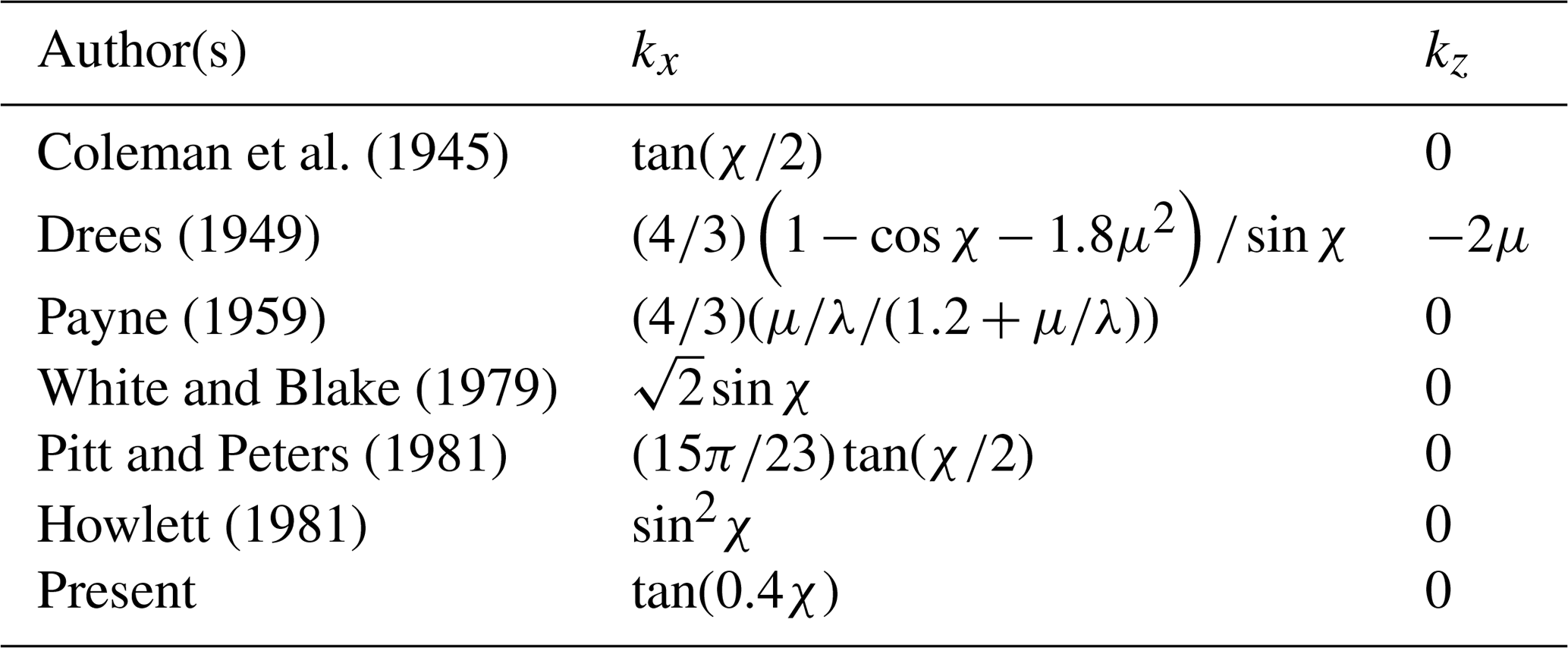
This is close to the model of Coleman, as seen in Table 1.
2.5.3 Comparison of the yaw model with actuator disk results
In Figs. 8 and 9, the above-described yaw model is compared with actuator disk results for a uniform, prescribed loading with a thrust coefficient of 0.8. In the BEM simulations, the constant CT was prescribed as well.
As seen in Fig. 8, the axial wind speed distribution at the rotor disk is seen to match very well in the vertical plane (z–y plane), which clearly illustrates the good performance of Glauert's expression for the mean induction at different yaw angles. It should be noted the drop in velocity for the AD-CFD results close to the edge is probably caused by the strong vorticity shed at the edge due to the jump in loading at the edge of the AD.
Results for the horizontal plane are depicted in Fig. 9, and the slope of the velocity variation across the disk is seen to correlate well between the AD and the BEM yaw model. However, towards the rotor edge, the AD induction is higher on the side where the wake is deflected to.
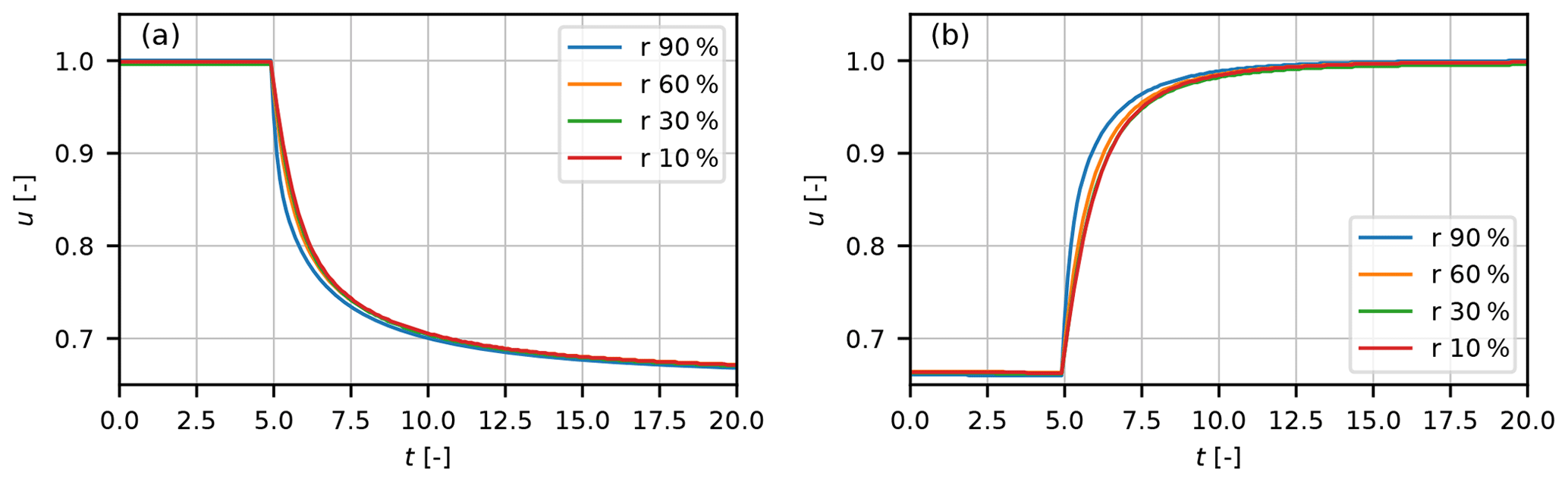
Figure 10The response of the axial velocity to a step change in loading at the actuator disk at different radial position. Panel (a) shows the response with CT from 0.0 to 0.89; panel (b) shows the response with CT from 0.89 to 0.0. The step change of loading is at t=5.
In summary, it can be concluded that the present yaw model is in close alignment with some of the models derived and presented in Schepers and Snel (1995). The Glauert correction for the mean induction seems to work very well, which was also the conclusion in Schepers and Snel (1995). The azimuthal variation seems to be well represented by the Coleman model but we found the coefficient 0.4 on χ instead of 0.5; see Table 1. However, one major difference by the present model is that, implemented together with the grid BEM induction model, we get a feedback on the induction from the yaw model which thus gives an additional azimuthal variation of the induction. This issue is addressed by Burton et al. (2011), mentioning that a lack of feedback is a contradiction in the derivation of, e.g., the Coleman model: constant loading (circulation) is assumed as a starting point but the solution is an azimuthal variation of induction and loading.
2.6 Dynamic inflow modeling
A time-varying loading of the AD will cause a time delay of the velocities at the disk as the whole wake flow has to adapt to the new loading. This phenomenon, the dynamic inflow effect, was also part of the abovementioned EU-funded project “Joint Investigation of Dynamic Inflow Effects and Implementation of an Engineering Method” (Schepers and Snel, 1995), where details about different modeling approaches can be found.
As for the yaw modeling, we use the AD-CFD model results again to develop and tune an engineering submodel for the dynamic inflow. The AD simulations are carried out with a uniform loading and a step change in CT from 0.0 to 0.89 and another case with opposite loading sequence from 0.89 to 0.0. The computed axial velocities u at the disk for different radial positions are shown in Fig. 10 as function of non-dimensional time t (time divided by R∕U0). It should be mentioned that the step size response was normalized to the BEM result of 1 to 0.666 for a change in CT of 0.89 for the different radial positions. This is because the AD-CFD results even for a constant loading typically show a non-uniform flow profile with the lowest velocity of 0.655 at the tip and a higher velocity of 0.695 at the center. This non-uniform velocity profile for a constant loading has been found and discussed by several authors: Madsen (1997), Madsen et al. (2010a), Sørensen et al. (1998) and Van Kuik (2018).
Comparing the decay in velocity for the different radial positions in Fig. 10a, it can be seen that the decay is slightly faster towards the tip than at the center. Likewise, the increase in velocity for decreasing step loading is also slightly faster at the tip, as seen in Fig. 10b. The physical mechanism for this small difference in flow response along the radius is that the change in the constant loading sheds a vortex at the edge of the AD with strongest and fastest induction response in the edge region.
Approximating the response with an engineering model led to the conclusion that two time constants are necessary to obtain an accurate fitting to the AD data. We use the following expression for the two first-order filters:
Here, u(t, r)`is the flow speed at time t at radius r, uav is the corresponding filtered flow speed, A1 and A2 are weighting constants of the two filters, τ1 and τ2 are the two time constants, and finally f1(a) and f2(a) are functions that adapt the time constants to the local flow speed depending on the induction factor a. The functions take the form
where and are constants.
We use a numerical optimization routine to find the set of parameters that minimizes the difference between the AD-CFD step response curves in Fig. 10 and the results of the model in Eq. (24). The variations of the two time constants along the radius are approximated with second-order polynomials in a non-dimensional radius.
The optimization gave the following polynomials for the time constants:
The τ functions are shown in Fig. 11a. It can be seen that while the highest time constant shows almost no variation along the radial distance, the lowest time constant decreases towards the tip, which corresponds to the faster flow response towards the tip as described above.
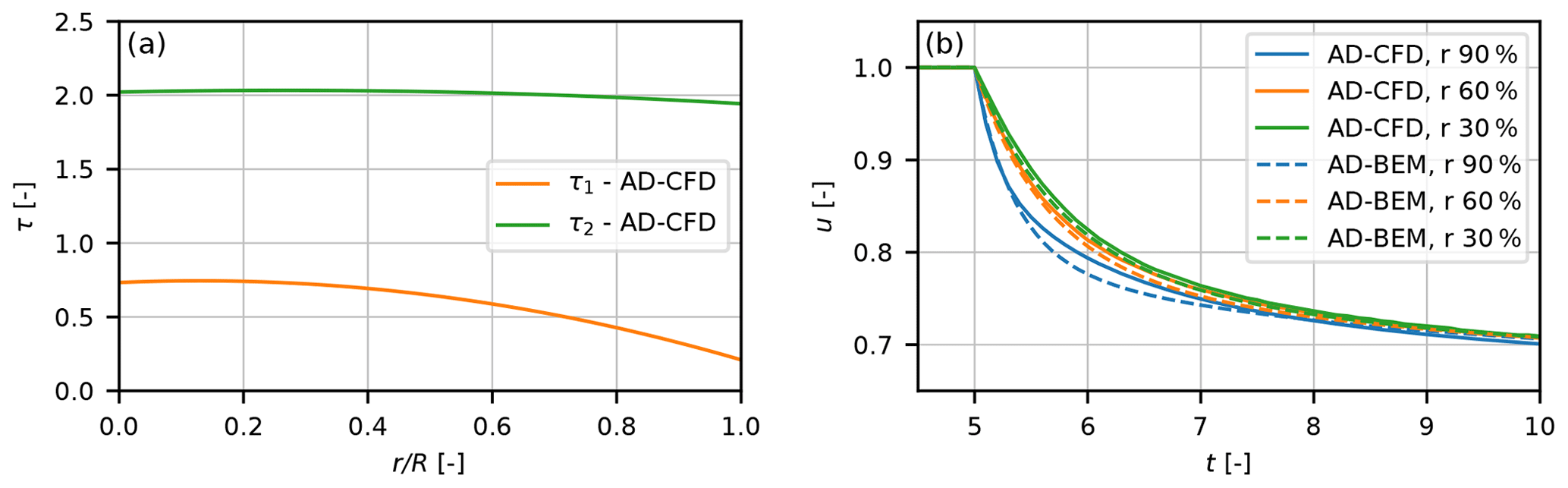
Figure 11(a) Figure showing the derived time constants as a function of non-dimensional radius. (b) Comparison of the step response of the model using tuned constants with the AD-CFD simulations.
A further result of the optimization is the weighting constants of the two filters which gave the following result:
Finally, the functions for the local flow speed to adjust the time constants were determined as
This result shows that the highest time constant (τ2) has to be scaled with a velocity very close to the wake flow velocity of 1−2a, whereas τ1 is scaled with a flow velocity that is between the flow velocity at the rotor disk (1−a) and the free-stream velocity. The induction factor a is limited to a maximum value of 0.4 in Eq. (28) to avoid unphysical behavior in the turbulent wake state.
As a test case of the implementation of the above-described dynamic inflow model implemented in the HAWC2 model, we run the same prescribed variation of CT as used above to derive the time constants. The comparison of the AD and HAWC2 model results in Fig. 11 shows a very good correlation, as should be expected. This is in good agreement with the work by Yu (2018), who derived a two-time-constant dynamic inflow model based on vortex models of an actuator disk.
In a time-marching formulation with non-dimensional time step δt (time step divided by R∕U0), the dynamic inflow filter at each grid point can be implemented as follows:
where the superscripts t and t−1 denote the present and previous time steps, and is the quasi-steady-induced velocity including the yaw correction (Eq. 22).
2.6.1 Summary on dynamic inflow
Comparing the present dynamic inflow model with the models derived and presented in Schepers and Snel (1995), we again find close correlation as for the yaw models. Firstly, the AD results clearly indicate that two time constants are needed where the highest constant is almost independent of radial position but the low one decreases towards the tip. The need of two time constants was also found in Schepers and Snel (1995) using the cylindrical vortex models. Secondly, we find that the time constants need to be normalized with a local convection velocity, which we found to be quite different for the two time constants. This was also the case for some of the models in Schepers and Snel (1995).
2.7 In-plane sweep and out-of-plane bending
For non-straight blades with sweep/prebend or in-plane and out-of-plane deflection, the radial distance between adjacent grid points is not equal to the distance along the curved blade. Therefore, both CT (Eq. 3) and CQ (Eq. 4) have to be multiplied with ds∕dr, the derivative of the blade span with respect to the radius.
The calculation of ds∕dr is demonstrated in the rotor coordinate system; see Fig. 12. The y axis is pointing downwind and the theoretical BEM rotor disk is in the x–z plane. The curved blade is represented by the half-chord line. The vector a is tangent to the half-chord line at this section point S. The vector r is pointing from the root point O to the section point S. The projection of vector r to the rotor plane (x–z plane) is b. It is equivalent to setting the y component of r to zero.
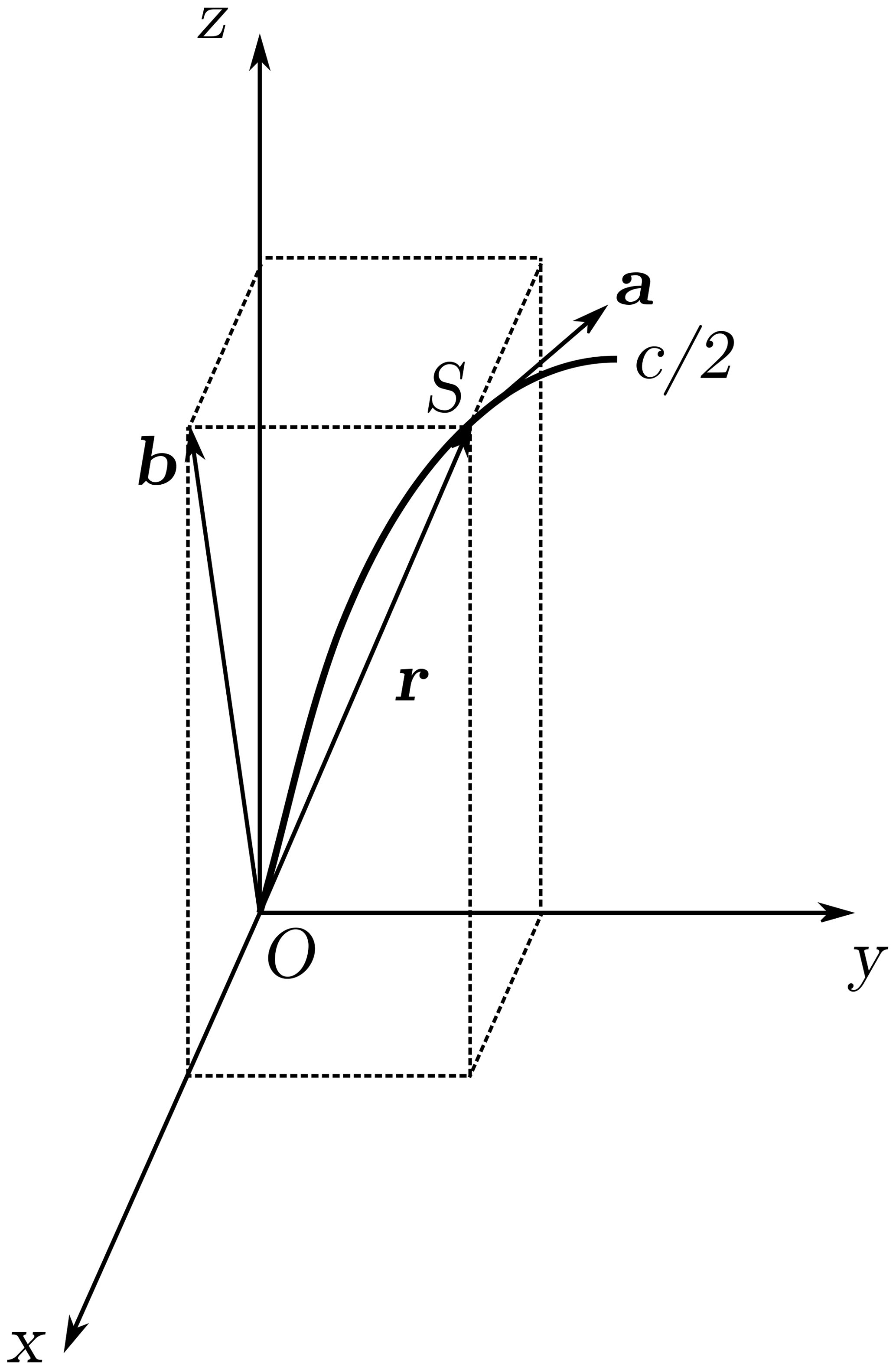
The curved length s is increasing in the direction of a, and the radius is increasing in the direction of b. Thus, ds∕dr can be calculated as
2.8 Radial induction model
The standard BEM theory does not give information about the radial induction component, and for plane rotors this induction component will only have minor influence on the loading. However, for rotors with out-of-plane bending blades or rotors with coning, the radial induction component will have an impact on the angle of attack (AOA) and thus also on the loading. An analytical expression for the lateral induction for a 2-D actuator disk is presented in Madsen (1997) and is adopted for an axis-symmetric AD in Madsen et al. (2010a). The expression is
where CTav(r) is the mean thrust coefficient as function of radial position defined as
where the local thrust coefficient CT(r) is given in Eq. (3). The use of CTav(r) instead of the total thrust coefficient is important only when CT shows a strong variation as function of radial position.
We test the radial induction model by a comparison with the AD-CFD solution for a constant loading of CT=0.89. As seen in Fig. 13, the radial induction computed with the engineering submodel correlates very well with the AD-CFD result.
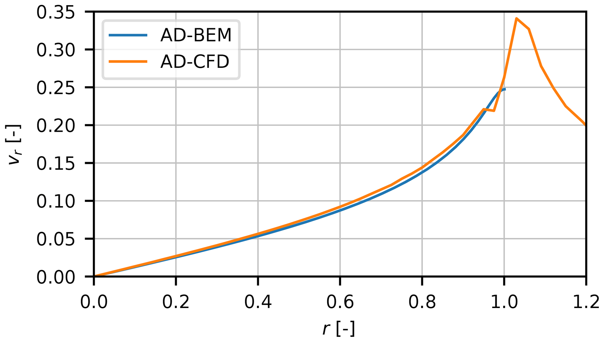
Figure 13The radial induction computed with an engineering submodel in comparison with the AD-CFD result for a constant loading with a thrust coefficient of 0.89.
2.9 Overview of the model
An overview of the complete aerodynamic model is shown in Algorithm 1. The algorithm includes references to the relevant equations in this article and can be used as a manual for implementation of the grid BEM algorithm. It is crucial that the dynamic inflow filter is applied at the very end of the algorithm to prevent nonphysical rapid induction changes due to any of the submodels. Otherwise, for example, a change in yaw angle at one time instant at the rotor disk in turbulent inflow would lead to an immediate change of the induced velocities, even though the wake did not have time to deflect.
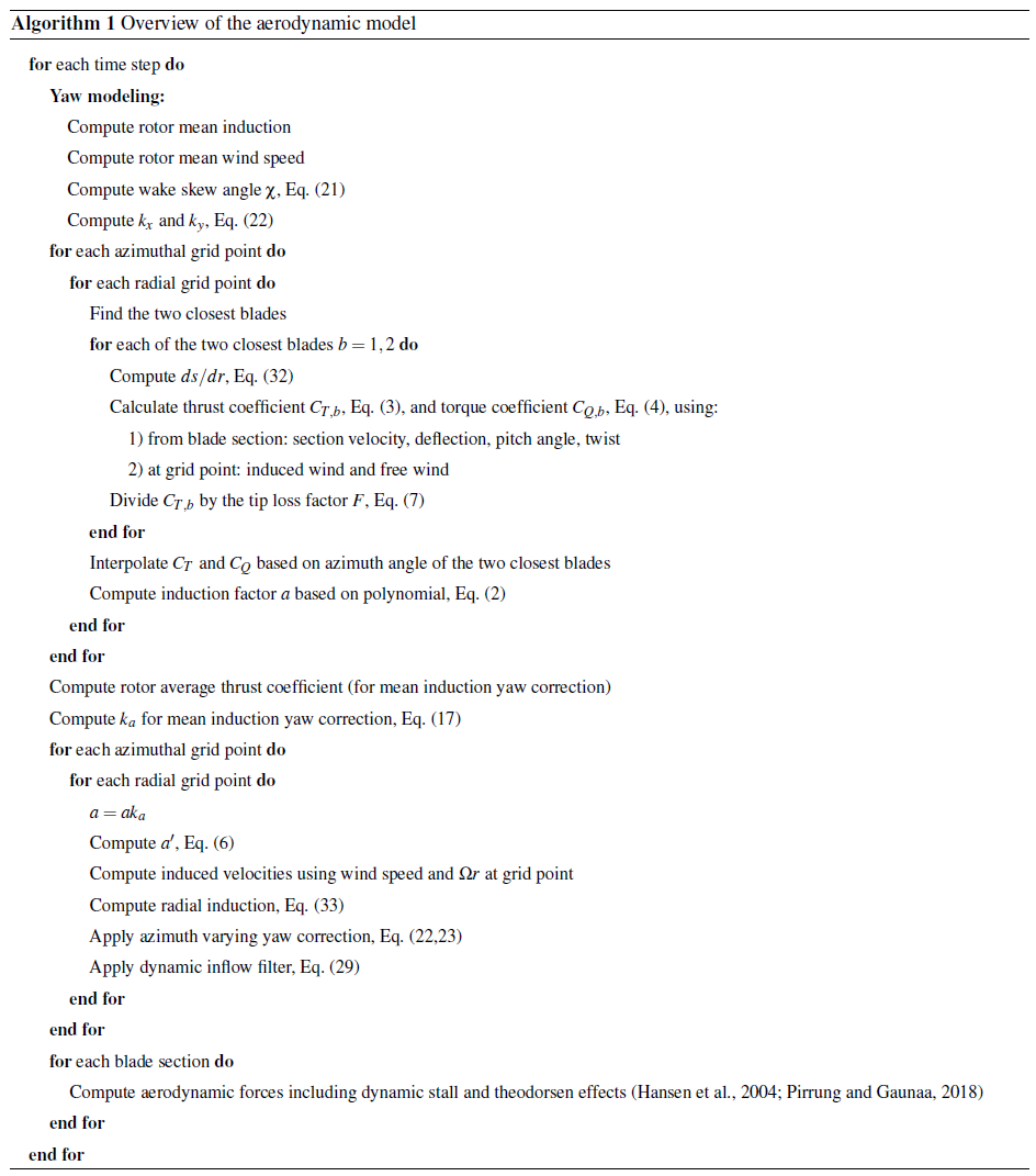
For a typical setup, we use 16 azimuthal grid points. The number of radial grid points are somewhat dependent on the planform and tip shape but typically 30–50.
The aerodynamic model as described here is the aerodynamic model in HAWC2. However, it is also found in a stand-alone version HAWC2_Aero which can run the same type of simulations with turbulent inflow, pitch actions and rpm variations as HAWC2 but for a stiff structure. In this version, the simulation speed with all input/output operations is on the order of 7–10 times real time on a 2016 workstation laptop. This means that the computational time for the aerodynamic part is still small (10 %–20 %) relative to the total computational time for the aeroelastic simulations although we, in this BEM implementation, update the induction over the whole disk at each time step. One reason for this is that no sub-iterations in the induction modeling are necessary.
At very low rotor speeds below 0.1 rad s−1, the induction model is deactivated. At these rotor speeds, the rotor can no longer be modeled as a disk and the BEM model is reduced to a blade element theory (BET) model that computes the velocity triangles without induced velocities. Another option in HAWC2 is to use a near-wake trailed vorticity model to model induction in stand still and idling cases (Pirrung et al., 2017a).
Unsteady airfoil aerodynamics effects (dynamic stall and Theodorsen effects in attached flow) are not included in the computation of the induced velocities. This is possible because unsteady airfoil aerodynamics occur at much faster timescales with time constants that depend on the half chord divided by the relative speed. For comparison, the dynamic inflow time constants scale with the rotor diameter divided by the free wind speed. After the induced velocities are computed, the unsteady airfoil aerodynamics are determined using the Beddoes–Leishman-type model described by Hansen et al. (2004), which was recently extended by Pirrung and Gaunaa (2018).
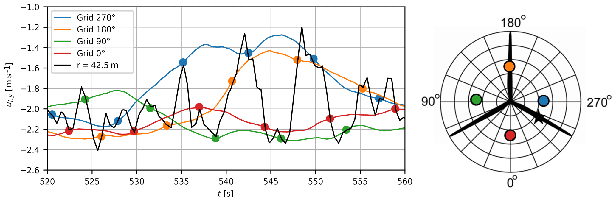
Figure 14Illustration of the dynamic induction mechanism in turbulent inflow showing the blade scanning through the field of slow-varying induction velocities but transferring to higher frequencies due to the rotational sampling of the turbulence.
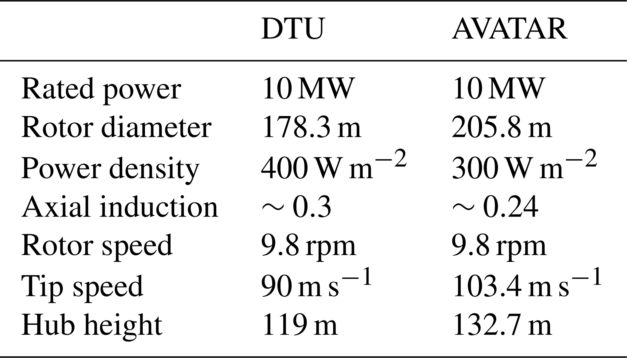
In this section, we demonstrate the impact of the present grid BEM implementation on the induction and load characteristics based on simulations of the AVATAR 10 MW reference wind turbine (RWT) (Sieros et al., 2015) and the DTU 10 MW RWT (Bak and Zahle, 2013) in turbulent and sheared inflow. The main data for these turbines are presented in Table 2.
Table 2Data for the DTU and AVATAR 10 MW reference wind turbines (Schepers et al., 2018a).
The impact is evaluated by comparing with an “annular mean BEM” version computing the mean induced velocities in an annular element. This annular mean BEM version was incorporated in a test version of HAWC2 for the present investigation. Because the version is only a test version, the mean annular approach was implemented in a crude way by executing the loop two times. During the first loop, the local three wind speed components were summed in new variables for each grid point. At the end of the first loop, the mean of the velocity components for a constants radius (a ring element) was derived and then used in the second loop instead of the local wind speed components.
3.1 The induction mechanism for turbulent inflow
The induction mechanism simulated with the grid BEM implementation for turbulent inflow is illustrated in Fig. 14. The simulations were carried out on the AVATAR turbine (Sieros et al., 2015) with a 205 m diameter rotor at 10 m s−1 and a turbulence intensity of 15 %, no shear and constant rotor speed. In the left panel of Fig. 14, we show the induced velocities at four grid points on the stationary rotor grid at a radius of 42.5 m with the monitoring points shown on the grid to the right. The induced velocities can be seen to vary slowly in time. They can be quite different in some periods due to the large turbulence scales causing different inflow velocities over the rotor. However, the induction seen from the rotating blade varies considerably faster, as it samples the induced velocities at the different azimuth grid positions. This rotational sampling of the induction field is thus basically the same mechanism as the rotational sampling of turbulence.
An important mechanism of the induction of the presented BEM implementation on a polar grid is that each grid point has a memory effect incorporated. Thus, past loading changes at a grid point (e.g., due to a pitch action in this region, a local gust, an instantaneous shear, a blade passing with another pitch angle offset) will influence the induction of the blade passing that grid point. The weighting of the impact of these past events is controlled by the dynamic inflow filter.
3.2 Characteristics of the induced velocities
To illustrate further the characteristics of the induced velocities from the AVATAR rotor case mentioned above, the time trace of the induced velocity at a radius of 43 m is shown in Fig. 15a. Further is shown for comparison the induced velocity simulated with the annular mean BEM method. The dynamic characteristics are clearly completely different which is further explored by the power spectral density (PSD) spectra shown in Fig. 15b. The spectra of the induced velocity computed with the grid BEM model have distinct peaks at 1P, 2P, etc. and can be seen to have close resemblance with the spectrum of the axial free wind speed component relative to the blade at same radial position. As the rotational sampling of both the inflow and the induced velocity field has the same characteristics, it indicates that the induced velocity field over the rotor also has the same overall characteristics as the turbulent inflow, although considerably lower wind speeds.
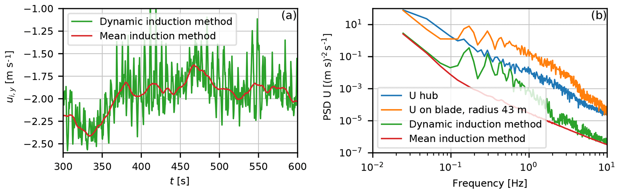
Figure 15(a) Time traces of induced velocity at a radius of 43 m simulated with the annular mean and grid BEM method. Panel (b) shows the PSD of the same two traces. Additionally, in the same figure, the PSD of the free wind speed relative to the blade at the same radial position and of the hub wind speed is shown. Clearly, the induced velocity at the blade exhibits 1P, 2P, …, nP peaks corresponding to the rotationally sampled turbulent inflow. These peaks can be observed on other radial positions on the blade as well.
As expected, the PSD of the induced velocity computed with the annular mean method has no peaks and has some resemblance with the PSD of the hub wind speed.
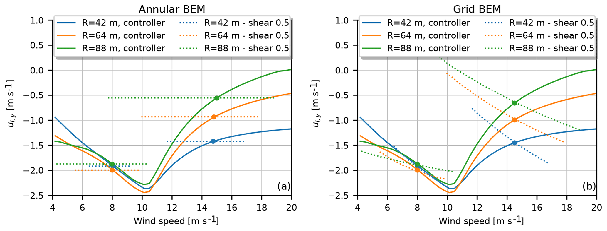
Figure 16(a) The results for the mean annular BEM model; (b) the grid BEM model results. The solid lines in both panels are the computed induction at three radial positions for the AVATAR rotor for a wind speed ramp from 4 to 20 m s−1 for uniform inflow and normal controller with variable speed and pitch regulation. The dashed lines are now the azimuthally varying induced velocities at the same radial positions for operation in sheared inflow with an exponent of 0.5 and at mean wind speeds of 8.0 and 14.5 m s−1, respectively.
3.3 Load impact mechanism of the grid BEM induction method
We will now illustrate the mechanism behind the load impact of using a mean annular BEM approach and a grid BEM model, respectively. Again, it is a simulation example for the AVATAR rotor.
A simulation was run with a ramp in wind speed from 4 to 20 m s−1 for uniform inflow. The induced velocities at three radial positions on the blade are shown in Fig. 16. As the inflow is uniform, both BEM implementations give the same result.
Now, a simulation is performed for sheared inflow with an exponent of 0.5 and at a wind speed of 8 and 14.5 m s−1, respectively. We show the induced velocity for the same radial positions on the blade as function of the local inflow velocity at that point.
For the mean annular BEM, the constant induced velocity as function of the local wind speed on the blade is obvious. The mean value might be slightly different from the value at the same wind speed for the turbine operating in uniform inflow due to non-linear effects from computation of the mean loading.
The picture is quite different for the grid BEM method, as shown in Fig. 16b. For all radial positions, at both wind speeds, we see that the induced velocity increases in magnitude but with the steepest slope at high wind. The mechanism behind this is that as soon as the inflow velocity is different from the hub wind speed the local blade section operates in conditions where either the rotational speed and/or the pitch does not correspond to the equilibrium conditions for that wind speed.
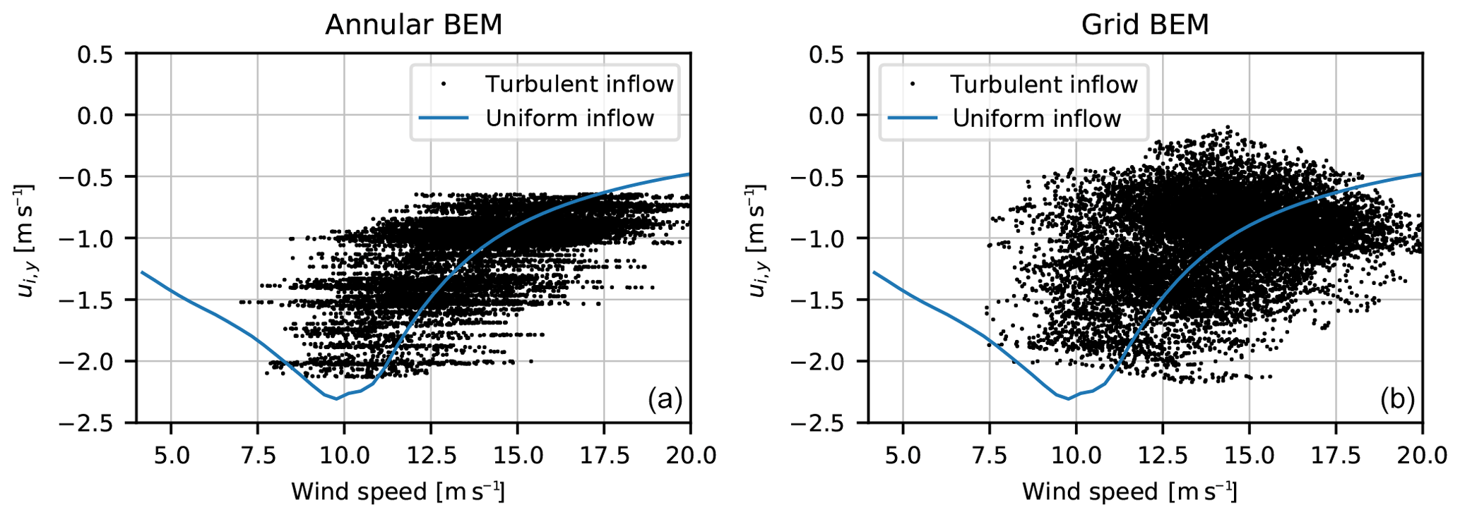
Figure 17(a) Results from the mean annular BEM; (b) results from the grid BEM. The solid lines in both panels are the computed induction at the radial position of 64 m for the AVATAR rotor for a wind speed ramp from 4 to 20 m s−1 for uniform inflow and normal controller with variable speed and pitch regulation. The dots are the induced velocities for turbulent inflow without shear for a mean wind speed of 14.5 m s−1.
At 8 m s−1, it is mainly the rpm that influences the variation in the local induction around the mean operational wind speed of 8 m s−1. When the local wind speed is lower than 8 m s−1, the local tip speed ratio is above the mean value and the blade section operates at a higher thrust coefficient. The opposite holds when the local wind speed is above the mean wind speed. The result is that the relation of the induction versus wind speed deviates from the induction curve for the turbine in uniform inflow. It also appears that the slope of this local relationship between induced wind speed ui,y and free local wind speed U0 decreases from root to tip. For local wind speeds below the operational point, the increased CT will increase the induced wind speed, whereas the decreased local wind speed (being a factor on the induction) will decrease the induced wind speed. In most conditions, the impact of the local wind speed multiplied on the induction factor is strongest but at high thrust coefficient regions towards the tip and for bigger deviations from the mean wind speed, we can see that the CT impact increases and the slope of the ui,y(U0) curve decreases. The slope can even be positive for very high thrust coefficients.
At 14.5 m s−1, it is mainly the pitch that influences the induction variation around the mean wind speed, as the rpm is constant for wind speeds above rated. So, when the blade section is in a region with a lower wind speed than the mean, the pitch is too high, which gives a lower thrust and a reduced induction. Opposite again when the local wind speed at the blade section is above the mean, the pitch is too low corresponding to that wind speed, which gives an increased induction. In this region, we can thus conclude that both the effect from the changes in CT and the variation in local wind speed when deviating from the mean operational point have the same sign, which means that we always will see a decreasing induction from a decreasing local wind speed and vice versa for a local wind speed above the mean operational point.
The important impact on the loads is that changes in the local wind speed will always be counteracted to some extent by the induced wind speed and thus reduce the variations in AOA and likewise variations of the aerodynamic loads. This will be further explored below for turbulent inflow and quantified for a few test cases.
3.4 Induced velocities for turbulent inflow
The characteristics of the induced velocities for turbulent inflow are basically determined by the same mechanism as described above for sheared inflow. As discussed above, the turbulent inflow with dimension of structures less than one rotor diameter cause a non-uniform inflow over the rotor disk. It means as for sheared inflow that a point on the rotating blade will see a local wind speed different from the mean wind speed corresponding to the mean operational conditions of the turbine. In Fig. 17, the induced velocity at radius 64 m is shown as function of wind speed for uniform inflow. The induced velocity as function of local wind speed from the same position on the blade for simulation with turbulent inflow at a mean wind speed at 14.5 m s−1 and a turbulence intensity of 15 % with standard control is shown as dots. Figure 17a shows the mean annular BEM, and Fig. 17b shows the grid BEM results. As the mean wind speed changes continuously for turbulent inflow, the ui,y(U0) curves as discussed above are more difficult to see here. However, for the mean annular BEM, the horizontal patterns of the dots are visible. For the grid BEM, we have to imagine that the ui,y(U0) curves have the negative slope, as shown above for shear at 14.5 m s−1.
3.5 Load and power impact for DLC 1.2 for the AVATAR and DTU reference wind turbine
The impact of the grid BEM model on fatigue loads and power production according to DLC 1.2 (IEC, 2005; Hansen et al., 2015) has been investigated. Computations were performed for both the DTU 10 MW RWT (Bak and Zahle, 2013) and the AVATAR 10 MW turbine (Sieros et al., 2015). To avoid seed dependency, 18 seeds at each wind speed were used: six seeds at 0∘ yaw error and six seeds at ±10∘ yaw error, respectively. The wind speeds range from 4 to 26 m s−1, with a 2 m s−1 spacing.
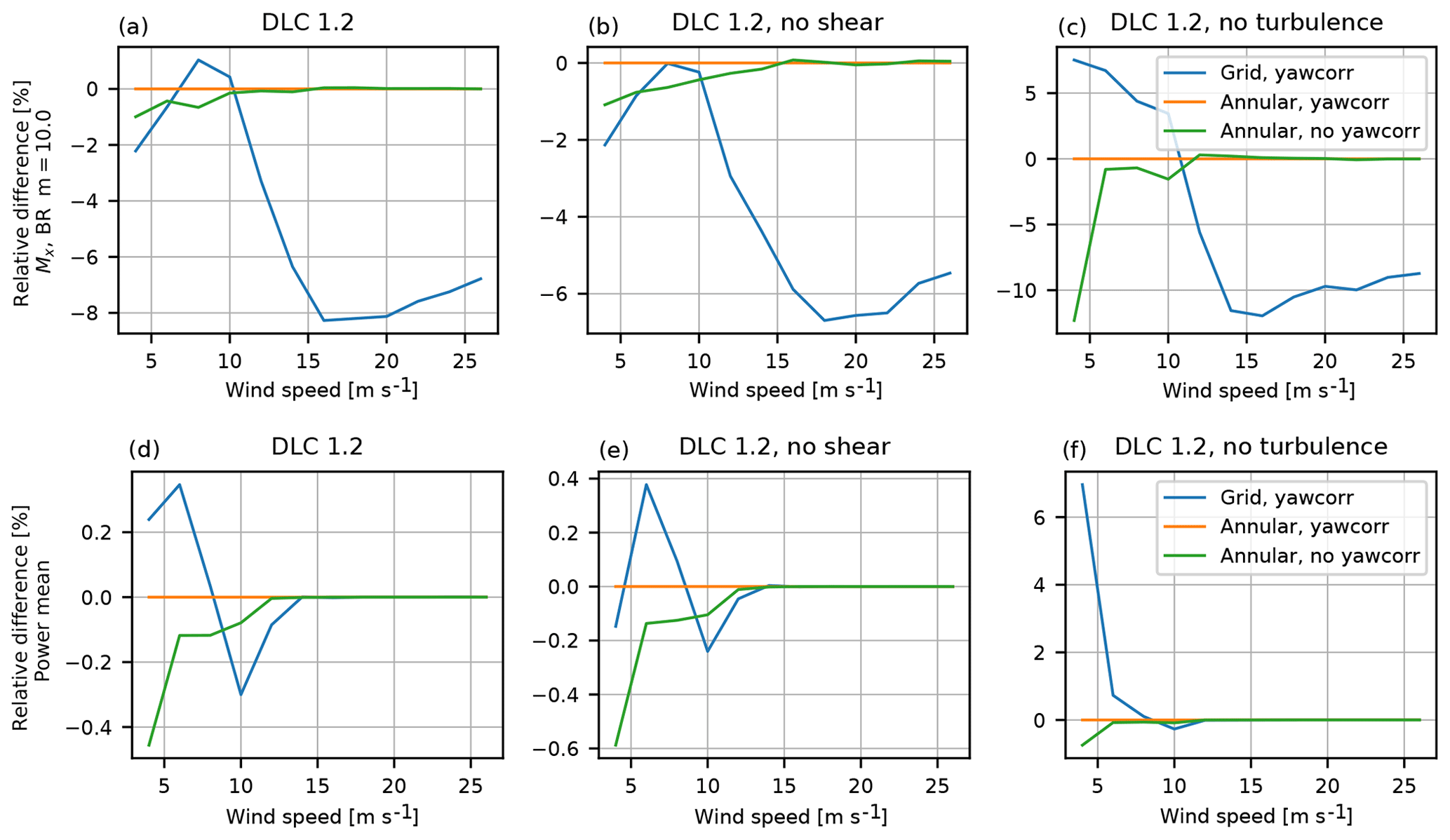
Figure 18A comparison for the DTU 10 MW RWT of the difference in blade root flapwise fatigue loads (a–c) and mean power production (d–f) for DLC 1.2 between the annular mean BEM method with and without yaw correction and the grid BEM version with yaw correction.
For brevity, this section focuses only on the 1 Hz equivalent load of the flapwise blade-root-bending moment and the mean power. All results are presented as percent relative difference compared to an annular BEM model that includes the yaw correction presented in Sect. 2.5. Results from a mean annular BEM model without yaw correction are also included so that the influence of grid versus mean annular BEM can be compared to the impact of a more widely used type of BEM model. To isolate the reaction of the induction model to shear and turbulence, additional runs of DLC 1.2 without shear and turbulence are shown. The runs without shear use the same 18 seeds per wind speed at 0∘ + 10∘ − 10∘ yaw error as the regular DLC 1.2 computations.
The results for the DTU 10 MW RWT are shown in Fig. 18. It can be seen that the difference of grid compared to annular BEM has a much larger impact on the results than the yaw correction. The yaw correction has some influence at wind speeds below rated, but above rated wind speeds, the influence is close to zero.
Overall, the grid BEM results in significant lower fatigue loads, up to 8 %, except in a narrow wind speed interval between 7 and 10 m s−1 with an increase of 1 %, as seen in Fig. 18a. When splitting up in contributions from turbulent inflow and shear, we can see in Fig. 18b that the fatigue from turbulence is reduced for all wind speeds for the grid BEM with a reduction of roughly 6 % at 16 m s−1 and above. However, for the impact from shear, the fatigue is increased up to 6 % at low wind speeds, which is due to the high thrust coefficient for that rotor, causing a positive slope of the ui,y(U0) curve as discussed above.
The influence of the grid-based BEM for the power production of the DTU 10 MW is very small at roughly ±0.3 % below rated. In the pure shear case at 4 m s−1, a large power increase by 6.5 % can be seen, but that increase almost disappears for combined turbulent and sheared inflow.
The results for the AVATAR turbine (Fig. 19) show a much larger impact of the grid BEM approach, while the yaw correction only has very minor influence. Relative to the annular BEM, the fatigue loads predicted by the grid BEM in pure shear are reduced on average by roughly 12 %, the loads in pure turbulence by 7.5 % and in the combined case by roughly 10 %. At the same time, the power below rated is predicted to increase by roughly 0.5 %, which seems to be mainly due to better operation in turbulent inflow.
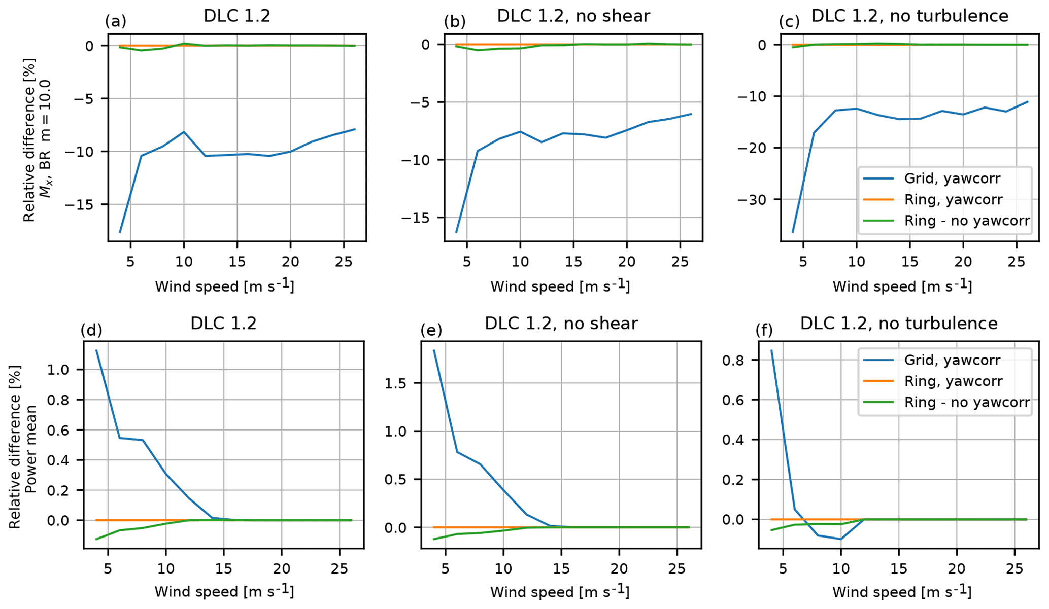
Figure 19A comparison for the AVATAR turbine of the difference in blade root flapwise fatigue loads (a–c) and mean power production (d–f) for DLC 1.2 between the annular mean BEM method with and without yaw correction and the grid BEM version with yaw correction.
Comparing the two cases, we can conclude that the impact of the grid BEM approach depends on the actual turbine design with an increasing reduction of fatigue loads for lower loaded (low-induction) rotors. For both turbine designs, the load reduction is considerable (8 % to 10 %) for wind speeds above rated power.
We present in this section a selection of validation results in order to illustrate the performance of the grid BEM implementation for different challenging inflow cases. As mentioned above, the grid BEM method is the aerodynamic model in HAWC2 and the cases are simulated with this model. It also means that several validation cases can be found in different articles published in the past and only two of them are explicitly summarized here. The first referenced validation paper contains not only a validation of the aerodynamic model of HAWC2 but of the full aeroelastic model. However, in the second validation reference, the aerodynamic model in HAWC2 is alternated between the grid BEM and full 3-D CFD, which enables a detailed validation of the grid BEM results.
4.1 Published validation cases
In Larsen et al. (2011), a validation study of both the HAWC2 model and the dynamic wake meandering (DWM) model (Larsen et al., 2008; Madsen et al., 2010c) was carried out on the basis of comparisons of model predictions with full-scale turbine measurements from the Dutch wind farm Egmond aan Zee consisting of 36 Vestas V90 turbines. In the paper, it is concluded that the measurements are of a remarkable high quality, enabling comparison of not only fatigue loads but also simple statistics in terms of maximum, minimum and mean values. It was found that when comparing the predicted power curves with measurements in both free and wake sectors, an excellent agreement is seen. Further, a very fine agreement was also seen between measured and simulated loads in both the free sector and a sector with wake effects from five turbines separated with seven diameters.
In the other validation publication by Heinz et al. (2016), the coupling of the HAWC2 structural model to EllipSys3D is presented. This provides an excellent basis for validation of the grid BEM aerodynamic model for simulations on the NREL 5 MW turbine (Jonkman et al., 2009), as a direct comparison with high-fidelity model results for the exact same input data and structural model is possible. Besides results for uniform inflow, a comparison of flapwise and edgewise tip deflection as function of azimuth is presented for 0, 30 and 60∘ yaw angles. In the paper, it is concluded that “both models still show a very good agreement”. Finally, a challenging case of an emergency shutdown is presented and also for that case it is concluded that the responses of the two models agree very well.
4.2 Half wake
The first validation case is to demonstrate the model response to a considerable shear in the inflow for the NREL 5 MW turbine (Jonkman et al., 2009). We have chosen a case with shear in the horizontal plane because a vertical shear representing atmospheric inflow with shear can be considerably influenced by the interaction of the flow with the ground surface and thus disturb the direct impact of the induction modeling (Madsen et al., 2010a). An artificial shear inflow was created by changing the inflow velocity from 10 to 5 m s−1 over a narrow region around the hub center, according to the following analytical expression:
where x is the horizontal distance from the rotor center, and R is the rotor radius. The resulting horizontal shear profile is shown in Fig. 21.
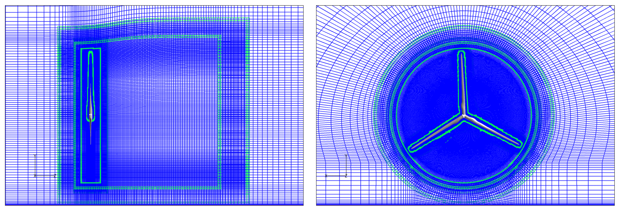
Figure 20Side view and front view of the CFD mesh around the NREL 5 MW reference turbine generated with a hub height of 90 m.
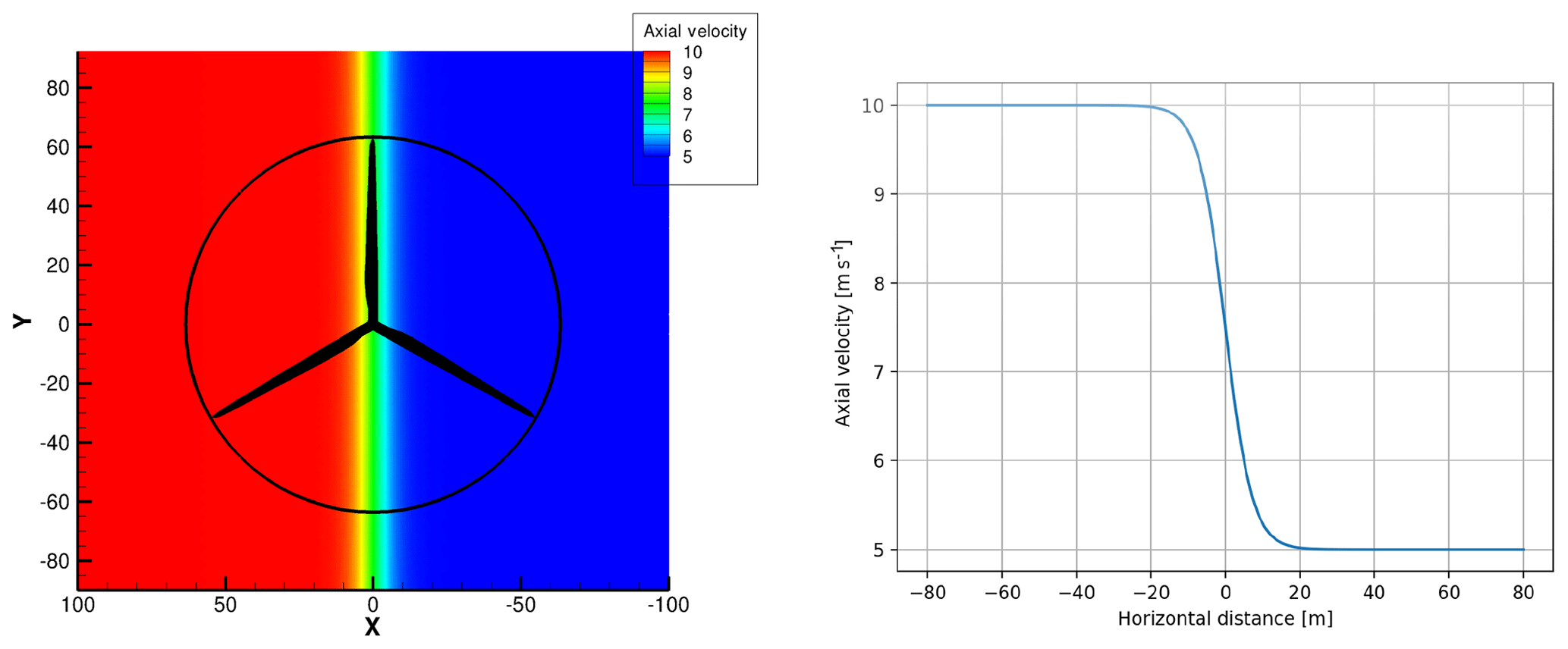
Figure 21The graph shows the contour plot for the velocity field for the sheared inflow case.
The CFD simulations were carried out with the 3-D incompressible Navier–Stokes solver EllipSys3D by Michelsen (1992, 1994) and Sørensen (1995), with a surface-resolved representation of the rotor, omitting the nacelle and tower. The flow on the no-slip surface of the rotor was assumed fully turbulent and modeled using the k−ω–SST model by Menter (1993). In the computations, we used an overset grid approach in which a curvilinear rotor resolved mesh rotated together with two successively coarsened cylindrical meshes resolving the near field around the rotor, which were embedded in a larger stationary coarse semi-cylindrical mesh resolving the far wake with the far-field boundaries placed eight rotor diameters away from the surface and a ground boundary modeled using a symmetry boundary condition placed 90 m below the rotor center. The surface of each blade was resolved with 256 cells in the chordwise direction and 128 cells in the spanwise direction, and grown into a volume mesh with 64 cells normal to the surface using the in-house hyperbolic mesh generator HypGrid (Sørensen, 1995). The first cell height was set to m, resulting in a y+ value below 2. The full grid assembly contained 15×106 cells. Figure 20 shows a front view and side view of the volume mesh.
To minimize the computational time, both grid sequencing and time step sequencing were used. To settle the overall induction field, the flow was simulated with a coarse time step of corresponding to 300 time steps per revolution for 20 revolutions on a mesh coarsened by a factor of 2 in each coordinate direction (Gr3). With the same mesh refinement level, the time step was subsequently refined by a factor of 5 to , yielding 1500 time steps per revolution for another 15 revolutions (Gr2). Finally, the mesh was refined to the finest grid level and the time step refined by a factor of 2 to (Gr1). The resulting mean integral forces of the grid/time step sequence are shown in Table 3.
Table 3Grid/time step convergence of the ElliPSys3D simulation, showing mean integral forces computed for the velocity step case at each of the three grid/time step levels.
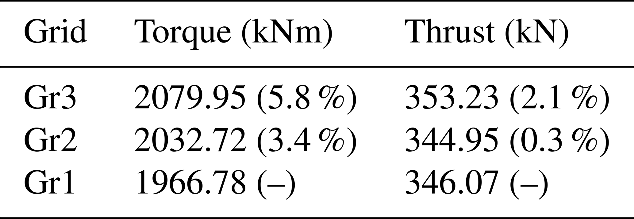
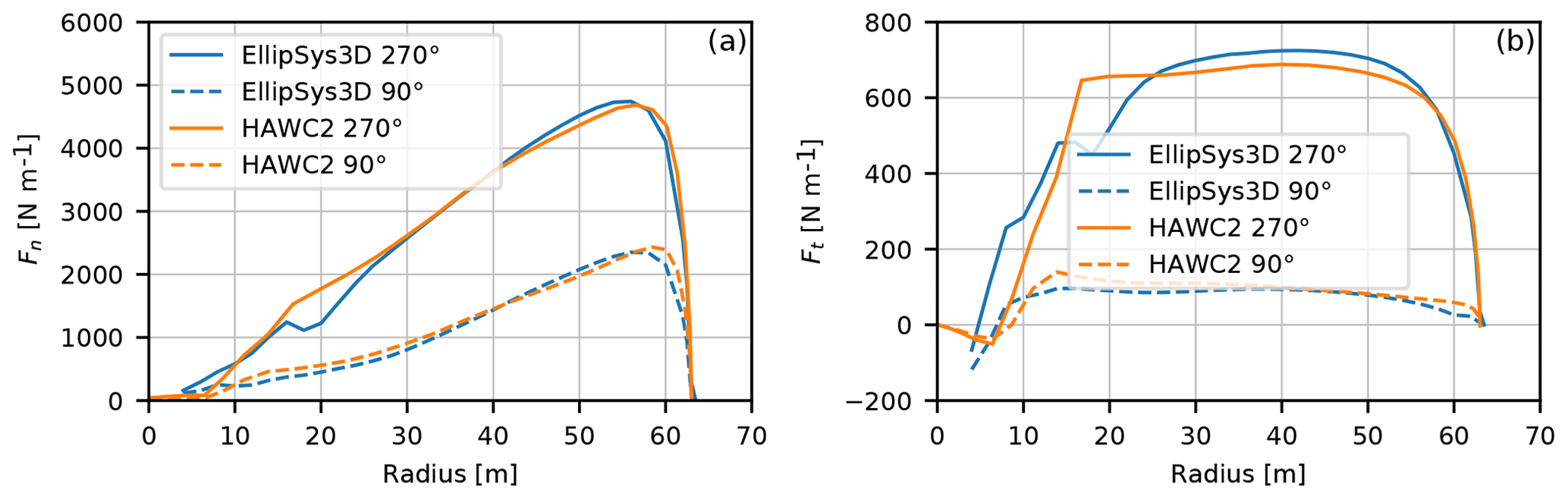
Figure 22The normal force (a) and tangential force (b) computed with HAWC2 at two azimuth positions in comparison with EllipSys3D results for half-wake inflow.
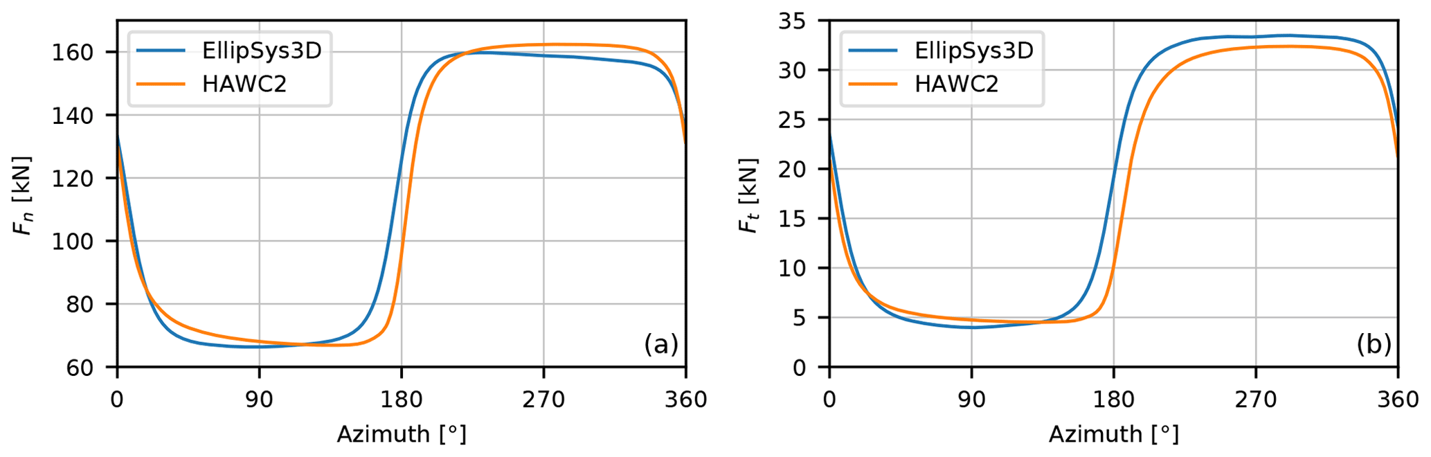
Figure 23(a) A comparison of the normal force Fn as function of azimuth computed with CFD and BEM, respectively. (b) Same comparison for the tangential force Ft.

Figure 24A comparison of HAWC2 simulations on the NM80 turbine and experimental results from the DanAero project. Power spectra of the chordwise aerodynamic force component parallel to the chord in comparison with measured results. Wind speed is 6.1 m s−1, negligible shear and rpm of 12.3. Figure reproduced from Madsen et al. (2018), with the addition of the annular mean BEM results.
A user-defined shear flow can be input to a HAWC2 simulation so the case could be simulated by a default setup. When comparing the normal and tangential loading on the blade at azimuth positions of 90 and 270∘ (0∘ is vertical upwards), which are in the extreme low and high inflow regions, we find overall a good correlation as can be seen in Fig. 22. There are minor deviations in the tip region where the grid BEM overestimates the normal force loading. Also, the tangential loading is slightly underestimated on the central part of the blade for the 270∘ azimuth position.
The case is further analyzed by comparing the integrated normal and tangential blade forces as function of azimuth as shown in Fig. 23. Again, an overall good correlation between the high-fidelity CFD results and the grid BEM results is found. However, there is a time delay for HAWC2 in the rising of the loads from low to high wind inflow (high to low CT) around an azimuth of 180∘. However, the same is not seen at around 0∘, where the wind speed is changing from a high to low value.
4.3 Turbulent inflow
Detailed aerodynamic measurements on full-scale turbines are very limited. However, in the DanAero project, such measurements were carried out in 2009 on a NM80 turbine with an 80 m diameter (Madsen et al., 2010b; Troldborg et al., 2014). The experimental setup comprised surface pressure measurements at four radial positions from which the aerodynamic forces normal and tangential to the local cord were derived. A validation exercise using these data was described and presented recently by Madsen et al. (2018), so we will only present a single set of results from that paper. The case is for a mean wind speed of 6.1 m s−1, a turbulence intensity of 6.8 % and minimal shear. For details of the experimental and modeling setup, the reader should see Madsen et al. (2018).
The comparison of PSD spectra of the measured and simulated aerodynamic forces perpendicular to the chord is shown in Fig. 24. Besides the grid BEM results, we have also added the mean annular results for comparison with the measurements. Overall, the correlation between simulations and measurements is good. In particular, the 1P, 2P and 3P peaks are captured well, and both simulation and experiment show the increasing size of the peaks towards the tip of the blade due to the rotation sampling effect of the turbulent inflow.
Figure 25Comparison of the differences in the azimuthal distribution of normal forces (a–c) and tangential forces (d–f) predicted by HAWC2 with the forces measured in the New Mexico experiment, at three different radial positions.
There is a clear tendency for the simulated spectra to fall below the measured one at higher frequencies, in particular for the outboard stations, which might be due to the resolution in the turbulence box which is 1.28 m in the vertical and horizontal directions. Finally, it can be seen that in this case the difference between the two BEM implementations is quite small. This can be explained by the above considerations in Sect. 4: if the local thrust coefficient is high, the slope of the ui,y(U0) curve in the grid BEM becomes almost horizontal and thus equal to the annular mean BEM. However, a light tendency of the annular mean BEM to overestimate the 1P and 2P on the two inboard stations with a lower thrust coefficient confirms the expected trend.
4.4 Yawed flow
In the New Mexico experiments (Boorsma and Schepers, 2018), the aerodynamic loading on a 4.5 m diameter model turbine in uniform inflow and yawed inflow was measured. These measurements have been compared to results from many aerodynamic codes of different fidelities in Schepers et al. (2018b). For a specific evaluation of the yaw modeling (Sect. 2.5), we look at the differences between the aerodynamic forces between the uniform and 30∘ yawed flow cases at roughly 15 m s−1 wind tunnel speed. In both cases, the turbine had a rotor speed of 425.1 rpm, the blades were pitched at −2.3∘, and the tunnel speed was very similar at 15.06 m s−1 (axial flow) and 15.01 m s−1 (yawed flow). As such, these measurements provide an excellent opportunity to validate the effect of yaw on both the mean and azimuthally varying load levels. Figure 25 shows the differences in normal (perpendicular to local chord) and tangential (parallel to local chord) forces at three measured sections at 25 %, 60 % and 82 % radius. These differences are computed as . Such a comparison involving both axial and yawed flow measurements and computations together was not included in Schepers et al. (2018b).

Figure 26Comparison of differences in out-of-plane (a) and in-plane blade-root-bending moments (b) predicted by HAWC2 with the moments integrated from the measured forces in the New Mexico experiment.
It can be seen that there is a phase shift in the azimuthal force variation between the normal forces at the inboard section (Fig. 25a) and the section further outboard (Fig. 25c). This phase shift is due to the dominance of either the root vortex (at the inboard section) or the tip vortex (outboard section). The root vortex is not accounted for in the present model, and thus the HAWC2 computations do not agree well with the measured normal force at the inboard section. A recent engineering model that is based on high-fidelity simulations and includes a correction for the root vortex is described by Rahimi et al. (2018).
For the sections further outboard, the influence of the tip vortex becomes more important and the phases of the azimuthal force variation agree well. There is a slight overprediction of the mean loading, especially in the tangential direction. Comparing the integrated out-of-plane and in-plane blade-root-bending moments in Fig. 26 shows that the phase difference seen in the inboard loads is not significant for the blade root moments. HAWC2 predicts a smaller reduction of the mean out-of-plane and in-plane moments, but the phases compare well to the measurements.
Figure 27Comparison of HAWC2 results against measurements of the dynamic inflow case Q0500000 of the NREL/NASA Ames phase VI experiment. The plots show scaled normal (a, c) and tangential (b, d) forces for pitch steps towards high loading (a, b) and low loading (c, d).
4.5 Dynamic inflow
The NREL/NASA Ames phase VI experiments (Hand et al., 2001), performed in the NASA Ames open-loop wind tunnel, include runs targeting dynamic inflow effects at 5.1 m s−1 wind tunnel speed (denoted as case Q0500000). The rotor speed was constant at 71.62 rpm and the pitch was varied 20 times at a rate of roughly 66∘ per second between −5.9∘ pitch (heavily loaded rotor, induction factor a≈0.5) and 10.02∘ pitch (unloaded rotor, a≈0). Averaging the responses of these 20 pitch steps shows pronounced dynamic inflow effects at all the instrumented blade sections at 30 %, 47 %, 63 %, 80 % and 95 % radius.
The measured data have been analyzed by Schepers (2007) using a BEM code and a free wake code and by Sørensen and Madsen (2006) using a BEM code, a computational fluid dynamics code and a near-wake model. More recently, this case was also used for comparison of various research codes in IEA Task 29, phase III (Schepers et al., 2018b). An investigation of the radial dependency of the time constants in the force response, which seemed to reverse when the pitching direction was reversed, was conducted by Pirrung and Madsen (2018).
A comparison of measurements with the dynamic inflow model described in Sect. 2.6 is shown in Fig. 27. All the forces are scaled such that the pitch steps are between 0 and 1. This approach makes it possible to compare the dynamic response at different sections on the blade easily and was also used by Schepers et al. (2018b). The computations assume a stiff turbine. It can be seen that the force overshoots at the 30 % section are generally larger than at the 80 % section. This is due to the slower response inboard due to the larger distance from the tip vortex. The dynamic inflow model takes this radial dependency of the time constants into account and the predicted overshoots of the forces are generally in good agreement with the measurements. An exception is that the overshoot of the tangential force at the inboard section (solid lines in Fig. 27b) is underestimated by HAWC2. The behavior of the tangential force for the pitching down case (Fig. 27d) can be explained by a zero crossing of the angle of attack at roughly 0.4 s. For both positive and negative AOAs close to 0∘, the lift force has a component that is pointing towards the leading edge. Therefore, the forces when pitching to lower loading are decreasing until the AOA reaches roughly zero. Then, the tangential forces increase as the AOA undershoots and then decrease again as the induced velocities decrease (causing AOA to increase and move closer to zero) towards the equilibrium state at low loading.
The comparison shows good agreement; however, some disagreement is to be expected due to inherent limitations of the actuator-disk-based model. Specifically, the root vortex dynamics are missing and the disk model also assumes an infinite number of blades. Therefore, differences are expected close to the root and the tip of the blade, where the induction from a helical wake deviates most from the induction due to a cylindrical wake. An option to address these limitations is to couple a vortex-based near-wake model to the BEM code (Pirrung et al., 2016, 2017b). However, the work in IEA Task 29 has shown that care has to be taken when coupling the induction dynamics (Schepers et al., 2018b).
We have presented an implementation of the BEM method on a polar grid in order to simulate more accurately the considerable inflow and load variations over the rotor disk found for large turbines. The model can also be characterized as an engineering actuator disk model where the induced velocities on the stationary polar grid are updated at each time step in an aeroelastic simulation. Further, the detailed integration of submodels for tip correction, yaw and dynamic inflow has been described. Also, a submodel for radial induction important for computations with out-of-plane blades due to elastic effects or coning has been presented.
The load impact mechanism on the flapwise blade root moment from this unsteady induction by the grid BEM is analyzed. It is found that the load impact strongly depends on the turbine design and operating conditions. For operation at low to medium thrust coefficients (conventional turbines at above rated wind speed or low-induction turbines in the whole operating range), it is found that the grid BEM gives typically 8 %–10 % lower 1 Hz blade root flapwise fatigue loads than the classical annular mean BEM approach. At high thrust coefficients, the grid BEM can give slightly increased fatigue loads, in particular for pure shear cases.
Different validation cases have been presented by comparing with experimental data and data from the high-fidelity EllipSys3D code. A challenging half wake in the vertical plane with the double inflow velocity on one side of the rotor relative to the other side is simulated. A good correlation is found with EllipSys3D results for blade loads as function of azimuth.
Results on yawed inflow for the Mexico rotor and dynamic inflow results from the NREL/NASA Ames experiment confirm a satisfactory performance of the submodels for yawed flow conditions and dynamic inflow. Finally, comparing PSD spectra of the simulated local aerodynamic forces at four radial positions on the full-scale NM80 turbine shows excellent agreement with spectra of measured forces originating from the DanAero experiment.
The data for most figures are openly available at: https://doi.org/10.5281/zenodo.3588359 (Madsen et al., 2019). Other data are available upon request.
| a | axial induction factor |
| a′ | tangential induction factor |
| A | rotor area |
| c | chord |
| Cd | sectional drag coefficient |
| Cl | sectional lift coefficient |
| CQ | rotor torque coefficient |
| CT | rotor thrust coefficient |
| Cx | projection of Cl and Cd tangential to the rotor plane |
| Cy | projection of Cl and Cd perpendicular to the rotor plane |
| dT | rotor thrust on a ring element |
| dQ | rotor torque on a ring element |
| F | Prandtl tip correction factor |
| k1, k2, k3 | polynomial coefficients in CT(a) curve fit |
| ka | reduction factor of induction for yawed flow |
| kx, ky | parameters for azimuth variation of induction in yaw model |
| NB | the number of blades |
| r | radial position |
| R | rotor radius |
| T | rotor thrust |
| TG→S | transformation matrix from global to sectional coordinates |
| ui,y | induced velocity vector in axial direction |
| u | non-dimensional axial velocity (velocity divided with U0) |
| U0 | free-stream velocity |
| free-stream velocity vector | |
| local free-stream velocity vector | |
| free wind speed vector at grid point (global coordinates) | |
| induced wind speed vector at grid point (global coordinates) | |
| resultant relative flow speed at grid point (section coordinates) | |
| Urel | relative velocity at blade section |
| blade velocity vector at grid point (global coordinates) | |
| Greek letters | |
| α | angle of attack |
| ρ | air density |
| φ | inflow angle |
| Φ | yaw angle |
| χ | wake skew angle |
| τ | time constant |
| Ψ | azimuth angle |
| ω | rotor speed |
HAM and TJL developed and implemented the overall grid BEM modeling approach. TJL tested the grid BEM model and increased the robustness of the implementation with contributions from GRP. HAM investigated the load mechanism of the grid BEM method. HAM performed the actuator disk simulations and extracted the data for tuning the yaw and dynamic inflow model. HAM, TJL and GRP wrote the article with contributions from FZ and AL. AL determined the time constants of the dynamic inflow model by means of numerical optimization. TJL and AL derived and implemented the correction for blade in-plane and out-of-plane bending. GRP executed and discussed the validation cases with major contributions from HAM. FZ derived the EllipSys3D setup for the half-wake simulations, conducted the simulations and extracted the data for the validation. All authors jointly finalized the paper.
HAWC2 is developed by DTU Wind Energy. The software can be licensed for research and commercial use.
We thank our colleagues in the AER and LAC section that in one way or another have contributed to this work and the modeling presented. In particular, we acknowledge the setup for automatic preprocessing and post-processing the DLC1.2 simulations presented in Sect. 4.5 developed by David Robert Verelst and Mads M. Pedersen. Also, the valuable contribution from Anders Melchior Hansen, one of the main developers of HAWC2, is acknowledged. We thank the two anonymous reviewers for the feedback. We also thank Frédéric Blondel from Ifpen and David Marten from TU Berlin for pointing out errors in the discussion article.
We also acknowledge the access to the New Mexico NREL/NASA Ames data in the IEA Task 29 database.
This paper was edited by Gerard J. W. van Bussel and reviewed by two anonymous referees.
Bak, C. and Zahle, F.: Description of the DTU 10 MW Reference Wind Turbine, Tech. Rep., Report-I-0092, DTU Wind Energy, Roskilde, Denmark, 2013. a, b
Boorsma, K. and Schepers, J.: New Mexico Experiment, Description of experimental setup, Tech. Rep. ECN-X–15-093 (v3), ECN, Petten, the Netherlands, 2018. a
Bossanyi, E.: GH Bladed Theory Manual. Technical Report, GH & Partners Ltd, Bristol, UK, 2003. a
Botasso, C. and Croce, A.: Cp-Lambda: Users Manual. Milano: Dipartimento di Ingegneria Aerospaziale, Polytecnico di Milano, Milano, 2006–2013. a
Burton, T., Jenkins, N., Sharpe, D., and Bossanyi, E.: Wind energy handbook, John Wiley & Sons, Chichester, UK, 2011. a, b, c
de Vries, O.: Fluid Dynamic Aspects of Wind Energy Conversion, Agardograph, Brussels, Belgium, 1979. a, b, c, d
Glauert, H.: Airplane Propellers, in: Division L in Aerodynamic Theory, vol. IV, edited by: Durand, W. F., Springer, Berlin, Germany, 169–360, 1935. a, b, c, d, e, f, g, h, i
Hand, M., Simms, D., Fingersh, L., Jager, D., Cotrell, J., Schreck, S., and Larwood, S.: Unsteady aerodynamics experiment phase VI: wind tunnel test configurations and available data campaigns, NREL/TP-500-29955, National Renewable Energy Laboratory, Golden, Colorado, USA, 2001. a, b, c
Hansen, M. H., Gaunaa, M., and Madsen, H. A.: A Beddoes-Leishman type dynamic stall model in state-space and indicial formulations, Risø-R-1354, Risø National Laboratory, Roskilde, Denmark, 2004. a
Hansen, M. H., Thomsen, K., Natarajan, A., and Barlas, A.: Design Load Basis for Onshore Turbines, No. 0174, DTU Wind Energy, Roskilde, Denmark, 2015. a, b
Hansen, M. O. L.: Aerodynamics of wind turbines, Earthscan, London, UK, https://doi.org/10.4324/9781315769981, 2015. a
Heinz, J. C., Sørensen, N. N., and Zahle, F.: Fluid-structure interaction computations for geometrically resolved rotor simulations using CFD, Wind Energy, 19, 2205–2221, https://doi.org/10.1002/we.1976, 2016. a
IEC: IEC 61400-1 3rd edition Wind turbines – Part 1: Design requirements, International Electrotechnical Commission – IEC, Geneva, Switzerland, 2005. a, b
Jonkman, J., Butterfield, S., Musial, W., and Scott, G.: Definition of a 5-MW Reference Wind Turbine for Offshore System Development, Tech. rep., National Renewable Energy Laboratory, Golden, Colorado, USA, 2009. a, b, c
Jonkman, J., Hayman, G., Jonkman, B., and Damiani, R.: AeroDyn v15 User's Guide and Theory Manual, NREL, Golden, Colorado, USA, 2016. a
Larsen, G. C., Madsen, H. A., Thomsen, K., and Larsen, T. J.: Wake meandering, Wind Energy, 11, 377–395, https://doi.org/10.1002/we.267, 2008. a, b
Larsen, T. J. and Hansen, A. M.: How 2 HAWC2, the user's manual, Risoe-R-1597, Forskningscenter Risoe, Risoe, Denmark, 2007. a, b
Larsen, T. J., Madsen, H. A., Larsen, G. C., and Hansen, K. S.: Validation of the dynamic wake meander model for loads and power production in the Egmond aan Zee wind farm, Wind Energy, 16, 605–624, https://doi.org/10.1002/we.1563, 2013. a
Leishman, J. G.: Principles of helicopter aerodynamics, Cambridge University Press, Cambridge, 2005. a, b, c
Madsen, H. A.: A CFD analysis of the actuator disc flow compared with momentum theory results, in: Proceedings of the 10th IEA meeting on aerodynamics, Edinburgh, UK, 109–124, 1997. a, b, c, d
Madsen, H. A.: Kobling af HawC til 3D actuator disc model, in: Chapter 5 in “Forskning i aeroelasticitet – EFP-98”, Risø National Laboratory, Roskilde, Denmark, p. 81, 1999. a, b
Madsen, H. A.: Yaw simulation using a 3D actuator disc model coupled to the aeroelastic code HawC, in: IEA Joint Action, Aerodynamics of Wind Turbines, 13. Symposium, 29–30 November 1999, Stockholm, 133–145, 2000. a
Madsen, H. A., Bak, C., Døssing, M., Mikkelsen, R. F., and Øye, S.: Validation and modification of the Blade Element Momentum theory based on comparisons with actuator disc simulations, Wind Energy, 13, 373–389, https://doi.org/10.1002/we.359, 2010a. a, b, c, d, e
Madsen, H. A., Bak, C., Schmidt Paulsen, U., Gaunaa, M., Fuglsang, P., Romblad, J., Olesen, N. A., Enevoldsen, P., Laursen, J., and Jensen, L.: The DAN-AERO MW Experiments, Risø National Laboratory, Roskilde, Denmark, 2010b. a
Madsen, H. A., Larsen, G. C., Larsen, T. J., Troldborg, N., and Mikkelsen, R. F.: Calibration and Validation of the Dynamic Wake Meandering Model for Implementation in an Aeroelastic Code, J. Sol. Energy Eng., 132, 041014, https://doi.org/10.1115/1.4002555, 2010c. a, b
Madsen, H. A., Riziotis, V., Zahle, F., Hansen, M., Grasso, F., Larsen, T., POolitis, E., and Rasmussen, F.: Blade element momentum modeling of inflow with shear in comparison with advanced model results, Wind Energy, 15, 63–81, 2012. a
Madsen, H. A., Sørensen, N. N., Bak, C., Troldborg, N., and Pirrung, G.: Measured aerodynamic forces on a full scale 2 MW turbine in comparison with EllipSys3D and HAWC2 simulations, J. Phys.: Conf. Ser., 1037, 022011, https://doi.org/10.1088/1742-6596/1037/2/022011, 2018. a, b, c
Madsen, H. A., Larsen, T. J., Pirrung, G. R., Li, A., and Zahle, F.: Data supplement for Wind Energy Science Paper `Implementation of the blade element momentum model on a polar grid and its aeroelastic load impact' [Data set], Zenodo, https://doi.org/10.5281/zenodo.3588360, 2019. a
Mann, J.: The spatial structure of neutral atmospheric surface-layer turbulence, J. Fluid Mech., 273, 141–168, 1994. a
Menter, F. R.: Zonal two-equation k−ω models for aerodynamic flows, AIAA paper 93-2906, AIAA, Orlando, Florida, 1993. a
Michelsen, J. A.: Basis3D – a platform for development of multiblock PDE solvers, Tech. Rep. AFM 92-05, Technical University of Denmark, Lyngby, Denmark, 1992. a
Michelsen, J. A.: Block structured multigrid solution of 2D and 3D elliptic PDEs, Tech. Rep. AFM 94-06, Technical University of Denmark, Lyngby, Denmark, 1994. a
Øye, S.: FLEX4 simulation of wind turbine dynamics, in: Proceedings of the 28th IEA Meeting of Experts Concerning State of the Art of Aeroelastic Codes for Wind Turbine Calculations, Lyngby, Denmark, 1996. a
Pena Diaz, A., Gryning, S.-E., Hasager, C. B., and Courtney, M.: Extending the wind profile much higher than the surface layer, in: Ewec 2009 Proceedings Online, Marseille, France, available at: https://orbit.dtu.dk/en/publications/extending-the-wind-profile-much-higher-than-the-surface-layer (last access: 5 December 2019), 2009. a
Pirrung, G. R. and Gaunaa, M.: Dynamic stall model modifications to improve the modeling of vertical axis wind turbines, DTU Wind Energy E-0171, DTU Wind Energy, Roskilde, Denmark, 2018. a
Pirrung, G. R. and Madsen, H. A.: Dynamic inflow effects in measurements and high-fidelity computations, Wind Energ. Sci., 3, 545–551, https://doi.org/10.5194/wes-3-545-2018, 2018. a
Pirrung, G. R., Madsen, H. A., Taesong, K., and Heinz, J.: A coupled near and far wake model for wind turbine aerodynamics, Wind Energy, 19, 2053–2069, 2016. a
Pirrung, G. R., Madsen, H. A., and Schreck, S.: Trailed vorticity modeling for aeroelastic wind turbine simulations in standstill, Wind Energ. Sci., 2, 521–532, https://doi.org/10.5194/wes-2-521-2017, 2017a. a
Pirrung, G. R., Riziotis, V., Madsen, H., Hansen, M., and Kim, T.: Comparison of a coupled near- and far-wake model with a free-wake vortex code, Wind Energ. Sci., 2, 15–33, https://doi.org/10.5194/wes-2-15-2017, 2017b. a
Rahimi, H., Martinez Garcia, A., Stoevesandt, B., Peinke, J., and Schepers, G.: An engineering model for wind turbines under yawed conditions derived from high fidelity models, Wind Energy, 21, 618–633, https://doi.org/10.1002/we.2182, 2018. a
Riziotis, V. and Voustinas, S.: Gast: A General Aerodynamic and Structural Prediction Tool for Wind Turbines, in: Proceedings of the EWEC'97, Dublin, Ireland, 1997. a
Schepers, J. G.: IEA Wind Task XX: Dynamic Inflow effects at fast pitching steps on a wind turbine placed in the NASA-Ames wind tunnel, ECN-E-07-085, ECN, Petten, the Netherlands, 2007. a
Schepers, J. G. and Snel, H.: Joint investigation of dynamic inflow effects and implementation of an engineering method, ECN-C-94-107, Petten, the Netherlands, 1995. a, b, c, d, e, f, g, h, i
Schepers, J. G., Boorsma, K., Sorensen, N., Voutsinas, S., Sieros, G., Rahimi, H., Heisselmann, H., Jost, E., Lutz, T., Maeder, T., Gonzalez, A., Ferreira, C., Stoevesandt, B., Barakos, G., Lampropoulos, N., Croce, A., and Madsen, J.: Final results from the EU project AVATAR: aerodynamic modelling of 10 MW wind turbines, J. Phys.: Conf. Ser., 1037, 022013, https://doi.org/10.1088/1742-6596/1037/2/022013, 2018a. a, b
Schepers, J. G., Lutz, T., Boorsma, K., Gomez-Iradi, S., Herraez, I., Oggiano, L., Rahimi, H., Schaffarczyk, P., Pirrung, G. R., Madsen, H. A., Shen, W. Z., and Weihing, P.: Final Report of IEA Wind Task 29 Mexnext (Phase 3), ECN-E–18-003, ECN, Petten, the Netherlands, 2018b. a, b, c, d, e, f
Sharpe, D. J.: A general momentum theory applied to an energy-extracting actuator disc, Wind Energy, 7, 177–188, https://doi.org/10.1002/we.118, 2004. a
Sieros, G.,Lekou, D., Chortis, D., Chaviaropoulos, P., Munduate, X., Irisarri, A., Madsen, H. A., Yde, K., Thomsen, K., Stettner, M., Reijerkerk, M., Grasso, F., Savenije, R., Schepers, G., and Andersen, C. F.: AVATAR Deliverable D1.2 – Reference Blade Design, Tech. rep., ECN, Petten, the Netherlands, 2015. a, b, c, d
Sørensen, J. N.: General Momentum Theory for Horizontal Axis Wind Turbines, Springer, Cham, Switzerland, 2016. a, b, c
Sørensen, J. N., Shen, W. Z., and Munduate, X.: Analysis of wake states by a full-field Actuator disc model, Wind Energy, 1, 73–88, https://doi.org/10.1002/(SICI)1099-1824(199812)1:2<73::AID-WE12>3.0.CO;2-L, 1998. a
Sørensen, N. N.: General purpose flow solver applied to flow over hills, Tech. Rep. Risø-R-827(EN), Risoe National Laboratory, Risoe, 1995. a, b
Sørensen, N. N. and Madsen, H. A.: Modelling of transient wind turbine loads during pitch motion, European Wind Energy Association (EWEA), Athens, Greece, 2006. a
Stepniewski, W. Z. and Keys, C. N.: Rotary-wing aerodynamics, in: Volumes 1 and 2, Genral Publishing Company, Toronto, Ontario, Canada, 1984. a
Thirstrup Petersen, J.: The aeroelastic code HawC – model and comparisons, in: State of the Art of Aeroelastic Codes for Wind Turbine Calculations, Technical University of Denmark, Lyngby, Denmark, 129–135, 1996. a
Troldborg, N., Sørensen, J. N., Mikkelsen, R., and Sørensen, N.: A simple atmospheric boundary layer model applied to large eddy simulations of wind turbine wakes, Wind Energy, 17, 657–669, https://doi.org/10.1002/we.1608, 2014. a
Van Kuik, G.: The fluid dynamic basis for actuator disc and rotor theories, IOS press BV, Amsterdam, the Netherlands, https://doi.org/10.3233/978-1-61499-866-2-i, 2018. a
Wilson, R. and Lissaman, P.: Applied aerodynamics of wind power machines, Oregon State University, Oregon, 1974. a, b
WMC: FOCUS6 – The integrated wind turbine design suite, Knowledge Centre WMC, Wieringerwerf, the Netherlands, 2019. a
Yu, W.: The wake of an unsteady actuator disc, PhD thesis, Delft University of Technology, Delft, https://doi.org/10.4233/uuid:0e3a2402-585c-41b1-81cf-a35753076dfc, 2018. a
The requested paper has a corresponding corrigendum published. Please read the corrigendum first before downloading the article.
- Article
(8925 KB) - Full-text XML