the Creative Commons Attribution 4.0 License.
the Creative Commons Attribution 4.0 License.
 | 24 Aug 2020
Multi-lidar wind resource mapping in complex terrain
Nikola Vasiljević
Johannes Wagner
Steven P. Oncley
Scanning Doppler lidars have great potential for reducing uncertainty of wind resource estimation in complex terrain. Due to their scanning capabilities, they can measure at multiple locations over large areas. We demonstrate this ability with dual-Doppler lidar measurements of flow over two parallel ridges. The data have been collected using two pairs of scanning lidars operated in a dual-Doppler mode during the Perdigão 2017 measurement campaign. There the scanning lidars mapped the flow 80 m above ground level along two ridges, which are considered favorable for wind turbine siting. The measurements are validated with sonic wind measurements at each ridge. By analyzing the collected data, we found that wind speeds are on average 10 % higher over the southwest ridge compared to the northeast ridge. At the southwest ridge, the data show, for approach flow normal to the ridge, a change of 20 % in wind speed along the ridge. Fine differences like these are difficult to reproduce with computational flow models, as we demonstrate by comparing the lidar measurements with Weather Research and Forecasting large-eddy simulation (WRF-LES) results. For the measurement period, we have simulated the flow over the site using WRF-LES to compare how well the model can capture wind resources along the ridges. We used two model configurations. In the first configuration, surface drag is based purely on aerodynamic roughness, whereas in the second configuration forest canopy drag is also considered. We found that simulated winds are underestimated in WRF-LES runs with forest drag due to an unrealistic forest distribution on the ridge tops. The correlation of simulated and observed winds is, however, improved when the forest parameterization is applied. WRF-LES results without forest drag overestimated the wind resources over the southwest and northeast ridges by 6.5 % and 4.5 %, respectively. Overall, this study demonstrates the ability of scanning lidars to map wind resources in complex terrain.
- Article
(5659 KB) - Full-text XML
- BibTeX
- EndNote


Traditionally, wind resource assessment is done with mast-mounted cup or sonic anemometers. Nowadays, with the commercialization and increasing acceptance of remote-sensing devices such as lidars and sodars, this practice is changing due to the clear advantages of remote-sensing devices: they are easily deployed, can be cost-effective, avoid the requirement of building permits, and can measure at higher heights. However, mast-based instruments, especially sonic anemometers, are probably still better suited for turbulence measurements (Sathe and Mann, 2013).
Vertically profiling wind lidars gained popularity for the assessment of mean wind speeds and are getting recognized by international standards for wind resource and power performance assessments (Clifton et al., 2018). Most profiling lidars perform velocity–azimuth display (VAD) scans to estimate the horizontal velocity from line-of-sight (LOS) measurements under the assumption of horizontal homogeneity. However, this assumption is typically violated in complex terrain. Errors from profiling lidars can be up to 10 % when measuring in complex terrain, as shown by Bingöl et al. (2009). One solution to overcome this problem is to use several lidars that directly measure different components of the wind at the same location. Moreover, the deployment of several lidars with scanning capabilities allows the assessment of wind conditions over large areas (Vasiljević et al., 2019), which can give important insights into the spatial variability of flow over very complex terrain. Multi-lidars have been proven to have a high measurement accuracy in comparison studies with sonic anemometers (Pauscher et al., 2016). Moreover, many studies utilized the scanning capability to measure wind fields over large areas for wind energy purposes in assessing, for example, wind turbine wakes (Trujillo et al., 2011; Iungo et al., 2013; Bodini et al., 2017; Menke et al., 2018b), the inflow towards wind turbines (Mikkelsen et al., 2013; Simley et al., 2016; Mann et al., 2018), the influence of surface and terrain features on the flow (Lange et al., 2016; Mann et al., 2017), and atmospheric phenomena such as gravity waves (Palma et al., 2019).
In this publication, we use measurements from the Perdigão 2017 campaign (Fernando et al., 2019). For this measurement campaign, wind lidars were a key measurement technology for the assessment of the flow over the complex terrain site. In total, 7 profiling and 19 scanning lidars (SLs) were deployed. The present study focuses on a subset of the entire data collection containing measurements of wind resources along two ridges, which are favorable sites for wind turbines, at Perdigão.
The relevance of such measurements is especially important for complex terrain sites where the uncertainty of current flow models is high (Bechmann et al., 2011). Potential sources of error are the characterization of the roughness resulting from different types of canopies (Wagner et al., 2019a), the characterization of the stratification in the atmosphere (Palma et al., 2019), the description of the terrain (Lange et al., 2017; Berg et al., 2018), and model resolution which may not capture all important flow phenomena in complex terrain. Therefore creating a good measurement data set of the flow over such terrain is imperative to improving the models. In this study, we present dual-Doppler lidar measurements that aim to assess the wind resources along the ridges at Perdigão. The measurements are validated against mast-based ultrasonic anemometers along the ridges, and observed flow structures are analyzed. Moreover, the lidar measurements are compared to Weather Research and Forecasting large-eddy simulation (WRF-LES) simulations with and without a parametrization of forest drag (Wagner et al., 2019a, b) to test the model's capability of reproducing the observed flow structures. This comparison reveals large deviations in model data to the lidar measurements, which underlines the importance of in situ measurements in complex terrain.
The paper is organized in the following way: Sect. 2 gives an overview of the Perdigão field campaign including a description of lidar and mast measurements, and Sect. 3 presents the Weather Research and Forecasting (WRF) model setup. Section 4 introduces the applied data processing techniques. Results are presented in Sect. 5, followed by a discussion in Sect. 6. Conclusions are given in Sect. 7.
The Perdigão 2017 field campaign took place at a site centered at the village Vale do Cobrão, located in Portugal, close to the Spanish border. The main selection criterion for the site was a distinct terrain feature of two parallel ridges of 4 km in length (Fig. 1). The ridges are about 1.5 km apart, and the height difference from the valley bottom to the ridge tops is about 250 m. The northwest–southeast orientation of the ridges is perpendicular to the prevailing wind directions, which were assessed prior to the campaign with a 30 m measurement mast (Vasiljević et al., 2017).

Figure 1(a) Elevation map of the Perdigão site in the PT-TM06/ETRS89 coordinate system. (b) Tree height map. (c) View from the southwest of the ridges with lidar and sonic anemometer sampling positions and wind turbine at center of the southwest ridge.
During the 2017 campaign, measurement devices were set up with a very high density by a large international group of universities, research institutions, and industry partners. Instruments were operated from early 2017 until early 2018, with an intensive operation period (IOP) from 1 May to 15 June 2017. To map the flow over the measurement site, 186 three-component sonic anemometers were installed on 50 meteorological masts with heights up to 100 m. Furthermore, 26 wind lidars (7 profiling lidars and 19 scanning lidars) were deployed. A full overview of the campaign's objectives and instrumentation may be found in Fernando et al. (2019). For this study, we analyze measurements from four SLs and four measurement masts located on the ridge tops.
2.1 Lidar measurements
As mentioned above, for this study we analyze measurements of four out of the eight SLs that were operated by DTU during the measurement campaign. The SLs, of the type Leosphere Windcube 200S, were operated as WindScanners (Vasiljević et al., 2016). The WindScanner-specific modifications allow the measurement of complex trajectories and the synchronization of multiple systems. In the following sections we will describe the experiment layout design process; the deployment process, including the calibration procedure; and the design and configuration of the scanning trajectories.
2.1.1 Layout
Our focus was on measuring wind resources above the SW and the NE ridge since the ridge tops are areas characterized by high wind resources and thus often used as locations for wind turbine placement in complex terrain. Accordingly, a measurement scenario is designed probing wind resources above both ridges. The scanning scenario, the so-called ridge scan, is characterized by intersecting lidar beams along the transects following the SW and NE ridge for about 2 km at a height of 80 m a.g.l. (above ground level; Fig. 1). This layout presents an extension of the design of the 2015 campaign (Vasiljević et al., 2017). The altitude of 80 m is chosen to match the hub height of the wind turbine located on the SW ridge. With only a pair of lidars used to measure along each transect, it is not possible to resolve the vertical velocity component. Thus, the lidar positions and scan strategy needed to be chosen to keep the elevation angles of the laser beams as low as possible (preferably below 5∘). Furthermore, the intersecting angle between the laser beams must be at least 30∘. Having elevation angles below 5∘ ensures that the influence of the vertical wind component is kept below 0.5 % as cos(5∘) = 0.996. The in-field placement of the lidars is based on high-precision terrain data and orthophotos acquired prior to the Perdigão 2015 campaign (Vasiljević et al., 2017).
2.1.2 Deployment
After the SLs were positioned at their designated locations, their orientation and leveling were determined by mapping the lightning rods of measurement masts using the SLs' laser beams (Vasiljević, 2014, p. 157). Both the position of SLs and lighting rods had been measured with centimeter accuracy (Menke et al., 2019a). By comparing referenced and mapped positions, the leveling and orientation of the SLs were improved, resulting in a pointing accuracy of about 0.05∘. To retain the pointing accuracy, the target mapping was repeated several times during the campaign to ensure that the leveling and orientation of the SLs remained unchanged.
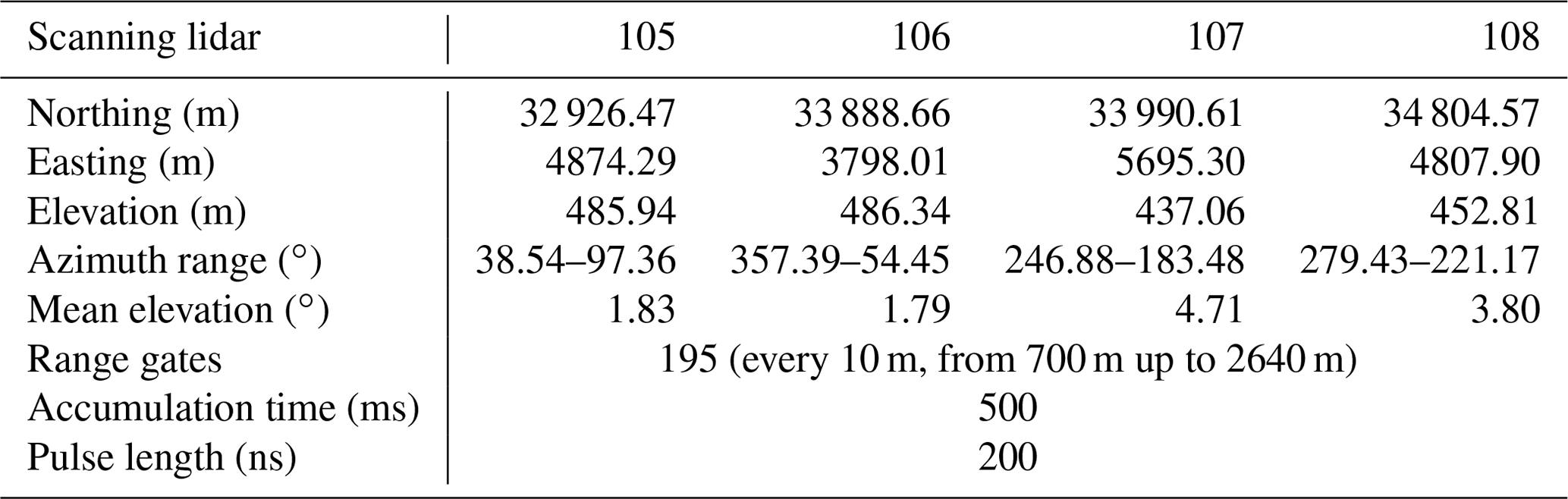
Table 1Scanning lidar coordinates and details about the measurement settings.
2.1.3 Scanning strategy
The two trajectories, which follow the ridge top line 80 m a.g.l., were designed using the high-precision terrain data. The traverses were 1.8 km long and described by points evenly spaced every 20 m. Accordingly we programmed the SLs to measure continuously along the trajectories by moving the beams through the trajectory points at a speed of 40 m s−1 and an accumulation time of 500 ms. As a result, spatial averaging takes place normal to the beam direction. Along the beam, range gates were placed every 10 m, starting at 700 m and extending to 2640 m (Table 1). Range gates represent slices (a certain number of samples) of the sampled backscattered light which are analyzed to estimate the wind vector component along the LOS. Each range gate corresponds to a spatial location for which the radial velocity is evaluated. The SLs were configured to emit 200 ns laser pulses and sample the resulting backscattered light with a frequency of 250 MHz. In the analysis of the backscattered light, each range gate is represented by 64 consecutive samples, resulting in a weighting function with a full width half maximum of about 30 m. One scan took 48 s, of which 45 s were spent on measurements, 0.5 s on acceleration and deceleration of the scanner heads, and 2 s on returning to the trajectory start point.
Typically, the WindScanner system uses a master computer to keep the synchronization of SLs to about 10 ms (Vasiljević et al., 2016). This synchronization requires a stable network connection between the SLs and the master computer. At the Perdigão site, due to the unstable network conditions, the SLs were configured to start the measurements in a scheduled fashion according to GPS time, thus independently from the master computer. This introduced time offsets due to a system-dependent start-up time which varies over time and among the different SLs. However, the SLs could perform measurements independent of the network connection, which results in higher data availability. The average time offset between SL 105 and 106 is 0.42 s ± 1.03 s and 0.7 s ± 0.65 s between SL 107 and 108.
2.2 Mast measurements
For this study, we use measurements from four masts: one 100 m mast located on the NE ridge as well as a 100 m and two 60 m masts that were located on the SW ridge. All masts are equipped with 3-D ultrasonic anemometers (Gill WindMaster Pro) and temperature and relative humidity sensors (NCAR SHT75) at the heights of 10, 20, 30, 40, and 60 m a.g.l. and 2, 10, 20, 40, and 60 m a.g.l., respectively. The 100 m masts also have ultrasonic anemometers and temperature and relative humidity sensors at 80 and 100 m a.g.l. Data were acquired at 20 samples per second with a 1 µs resolution GPS-based time stamp on every sample.
In this study, long-term simulations of Wagner et al. (2019a, b) are compared to lidar ridge scans to determine the quality of a numerical model over complex terrain. Model simulations were performed with the Weather Research and Forecasting (WRF) model (Skamarock et al., 2008) on three nested domains, D1 to D3, with horizontal resolutions of 5 km, 1 km, and 200 m, respectively. The innermost domain, D3, is run in large-eddy simulation (LES) mode. The LES setup was chosen to be independent of boundary layer parameterizations in domain D3, although a horizontal resolution of 200 m is relatively coarse for an LES run. Vertical nesting is applied to define individual levels in the vertical for each model domain (Daniels et al., 2016). For domains D1–D3, 36, 57, and 70 vertically stretched levels are used, and the respective lowest model levels are set to 80, 50, and 15 m a.g.l. The model top is defined at 200 hPa (about 12 km height) to include radiation and cloud effects at the tropopause. At the model top, a 3 km thick Rayleigh damping layer is applied to prevent wave reflection (Klemp et al., 2008). The simulation was initialized once at 00:00 UTC on 30 April 2017 and run for 49 d and 18 h, until 18:00 UTC on 18 June 2017. The initial and boundary conditions are supplied by the European Centre for Medium-Range Weather Forecasts' (ECMWF) operational analyses on 137 model levels with a horizontal resolution of 8 km and a temporal resolution of 6 h. The WRF output interval of domain D3 was set to 10 min. The complete model setup including the physical parameterizations that were used is described in detail in Wagner et al. (2019a, b). Two simulations were performed for the whole IOP of the Perdigão 2017 campaign and are run with (WRF_F) and without (WRF_NF) a forest parameterization in the LES domain D3. Without forest parameterization, surface drag is defined by an aerodynamic roughness length z0, which is obtained from the CORINE 2012 land use data set and converted to land use types according to Pineda et al. (2004). In the WRF_F run, an additional forest drag term following Shaw and Schumann (1992) is implemented, which decelerates the flow on the lowermost model levels. The forest cover and leaf area index (LAI) are retrieved from the CORINE data set. As no information about the tree height at the point of the model configuration was available, a randomly uniformly distributed forest height of 30 m ± 5 m is used for the modeling domains. The high-resolution aerial scans are only available for a smaller area centered around the measurement site (Fig. 1b). A detailed description of the forest parameterization and the differences between the WRF_F and WRF_NF simulations is given in Wagner et al. (2019b).
Model data of the LES domain D3 is available with a 10 min output interval. This means that every 10 min a snapshot of the simulated meteorological condition is written to the output file. The three-dimensional fields are interpolated linearly in both the horizontal and vertical direction to the lidar ridge scan coordinates. This results in time series of meteorological variables at each lidar scanning point, which can be compared to lidar data.
4.1 Mast data
The anemometer data are rotated into a vertical coordinate system (i.e., w is aligned with the vertical axis of the local coordinate system PT-TM06/ETRS89, which is also used for the lidar data) and oriented to true north from angles determined by laser multistation scans of each instrument. No issues are determined in the quality control process, so the reported data from the anemometers are used unedited.
The fans used to aspirate the temperature and relative humidity sensors on the masts occasionally failed during the project. Data from these periods were removed. Furthermore, for some of these sensors, laboratory postexperiment calibrations indicated larger-than-expected differences from the precalibrations (usually less than 0.5 ∘C and 4 % relative humidity). For these sensors, the postcalibrations are applied.
For the comparison of sonic and lidar measurements, we project the 80 m sonic wind speeds to the SL LOSs using Eq. (1) and calculate the sonic wind speed projected to the plane spanned by the two lidars. The former is calculated as
where Vr_sonic is the sonic wind speed projected to the individual LOSs of the SLs, and u, v, and w are the wind vector components. The sonic data are averaged exactly during the accumulation period (500 ms) of the SLs at the two closest range gates to the masts that are not affected by the measurement mast structures. These range gates are about 40 m to the northwest and southeast of the masts.
The latter, the sonic wind speed projected to the plane spanned by the two lidars, is used to investigate the correlation of horizontal wind speeds measured by the sonics and the lidars. For the sonic measurements, we consider the horizontal wind speed () and the wind speed projected to the plane spanned by the two lidars (), where the projected wind vector is calculated as
with n being the unit normal vector of the plane spanned by the two lidar beams.
Furthermore, the mast data are used to determine the atmospheric stability based on the Richardson number (Ri) calculated at the upstream mast as defined in Menke et al. (2019b) based on the potential temperature gradient from 20 to 100 m and the wind speed at 100 m. It is not obvious how to define limits for different stability regimes; thus we define stable conditions as periods with Ri>0 and unstable conditions as Ri<0. Neutral conditions are only expected to occur during short transition periods.
4.2 Lidar data
We process the lidar data in three consecutive steps. First, the data are filtered using the method described in Sect. 4.2.1. Next, the measurements of the filtered scans along the ridge trajectories are combined with horizontal winds (see Sect. 4.2.2). Finally, the combined measurements are averaged over 10 min periods.
4.2.1 Filtering
Most commonly, lidar data are filtered by thresholding using the carrier-to-noise ratio (CNR) as a quality indicator. These methods are described by Beck and Kühn (2017), who give a general overview of lidar data filtering approaches and also present highly innovative methods. Here we are proposing a new approach which is based on the assumption that the wind field has a certain degree of continuity. We filter the lidar data in a three-stage process that is applied to each scan: in stage one, the data are filtered based on a moving median value of the LOS velocities measured along each LOS. The median is calculated for a window that stretches over 15 range gates, corresponding to a distance of 150 m. All range gates that deviate by a threshold of 3 m s−1 from the median are excluded.
In stage two, all measurements that exceed the median of radial velocities along an entire LOS by a threshold value of 6 m s−1 are filtered out. Both thresholds were determined by visual inspections of plotted data and tuned to the present values. After each stage, missing range gates are linearly interpolated by the value of the two neighboring range gates in case they have valid values. In a final stage, range gates with valid values that are surrounded by three or more invalid range gates out of the two previous and two following range gates are excluded. These range gates are considered as scatter that is unlikely to have a valid measurement or have a meaningful contribution to the analysis. The first two stages are intended to remove local and global artifacts in the measurements. Finally, all filtering stages are repeated across LOSs in the azimuthal direction.

Figure 2Comparison of data recovery with different filters for the 10 min period starting on 3 May 2017 at 13:40 UTC. (a) Unfiltered data, (b) filtered data following the approach described in Sect. 4.2.1, (c) −27 dB filter, and (d) −24 dB filter.
We demonstrate the performance of this method compared to CNR filters with the thresholds of −24 and −27 dB (Fig. 2). Our approach recovers more data in the far range of the scans, thus extending the range of the scans during periods with low CNR, and can remove artifacts caused by, e.g., hard targets or second return pulses originating from, for example, a cloud base at a higher elevation. The average availability with our filtering approach is 91.8 % compared to 77.7 % (92.2 %) with a −24 dB (−27 dB) filter. The high availability of the −27 dB filter is misleading in the sense that this method does not remove all artifacts from the scans (compare Fig. 2c).
4.2.2 Wind vector reconstruction
The horizontal components of the wind vector (u positive east and v positive north) are reconstructed from measurements of the two SLs measuring along the same ridge. The measurements at the 92 ridge trajectory points are combined applying Eq. (3):
with Vr being the radial or LOS velocities measured by the two SLs; ϕ the azimuth angles using the geographical convention, i.e., 0∘ is pointing north, and ϕ increases clockwise; and ϑ the elevations angles of the scanners. In this calculation the influence of the vertical wind component w is considered to be negligible since we measured at low elevation angles. We combine 10 min averaged radial velocity components. Measurement points with fewer than 10 independent samples are disregarded as well as complete scans with more than 20 % invalid data.
4.2.3 Data availability
The four SLs were in operation for different periods from 22 March to 24 July. Individual system availability in these periods ranges from 59 % to 80 % (Table 2). During the IOP, due to the permanent presence of people at the site to aid in the case of a power grid or system failure, the SLs' availability is higher (71 % to 92 %). For dual-Doppler retrievals at the individual ridges, concurrent availability of SL 105 and SL 106 for the NE ridge and SL 107 and SL 108 for the SW ridge is required. The combined availability during the IOP is 79 % and 51 % for the NE and SW ridge, respectively. Simultaneous measurements at both ridges are available for 44 % of the period of the IOP. After applying filtering processes as explained in Sect. 4.2.1, the data availability reduces to 31.6 %. For the analysis, we only use measurements of the IOP period due to the higher data availability, and we removed periods with wind speeds below 3 m s−1 at 80 m height (measured at the mast tse04), which leaves 507 10 min periods, corresponding to 23 % of the IOP period.
Table 2Operation time and data availability of SLs. The number in brackets is the number of available 10 min periods.
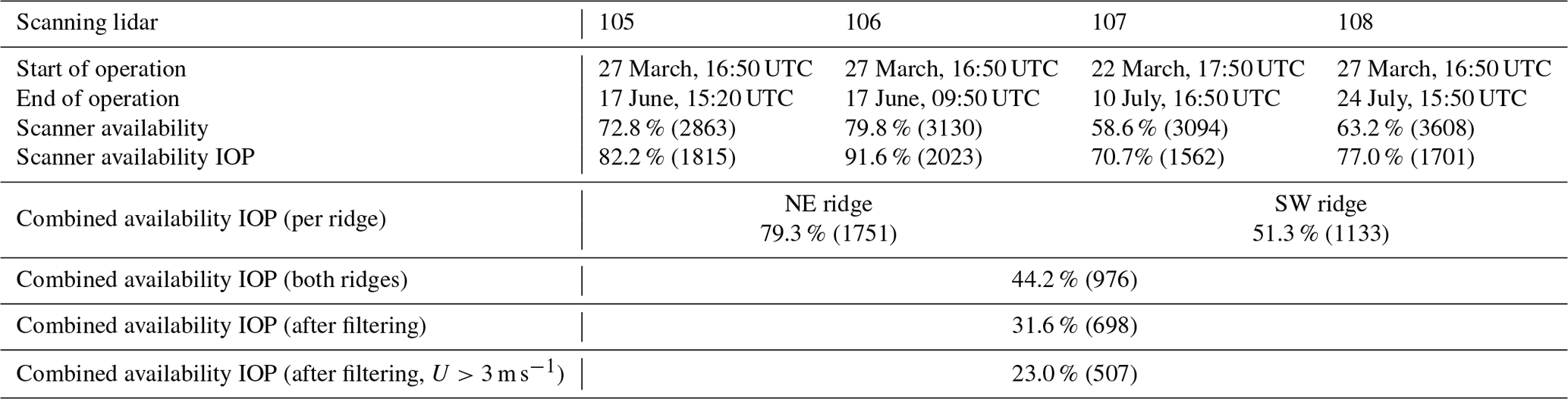
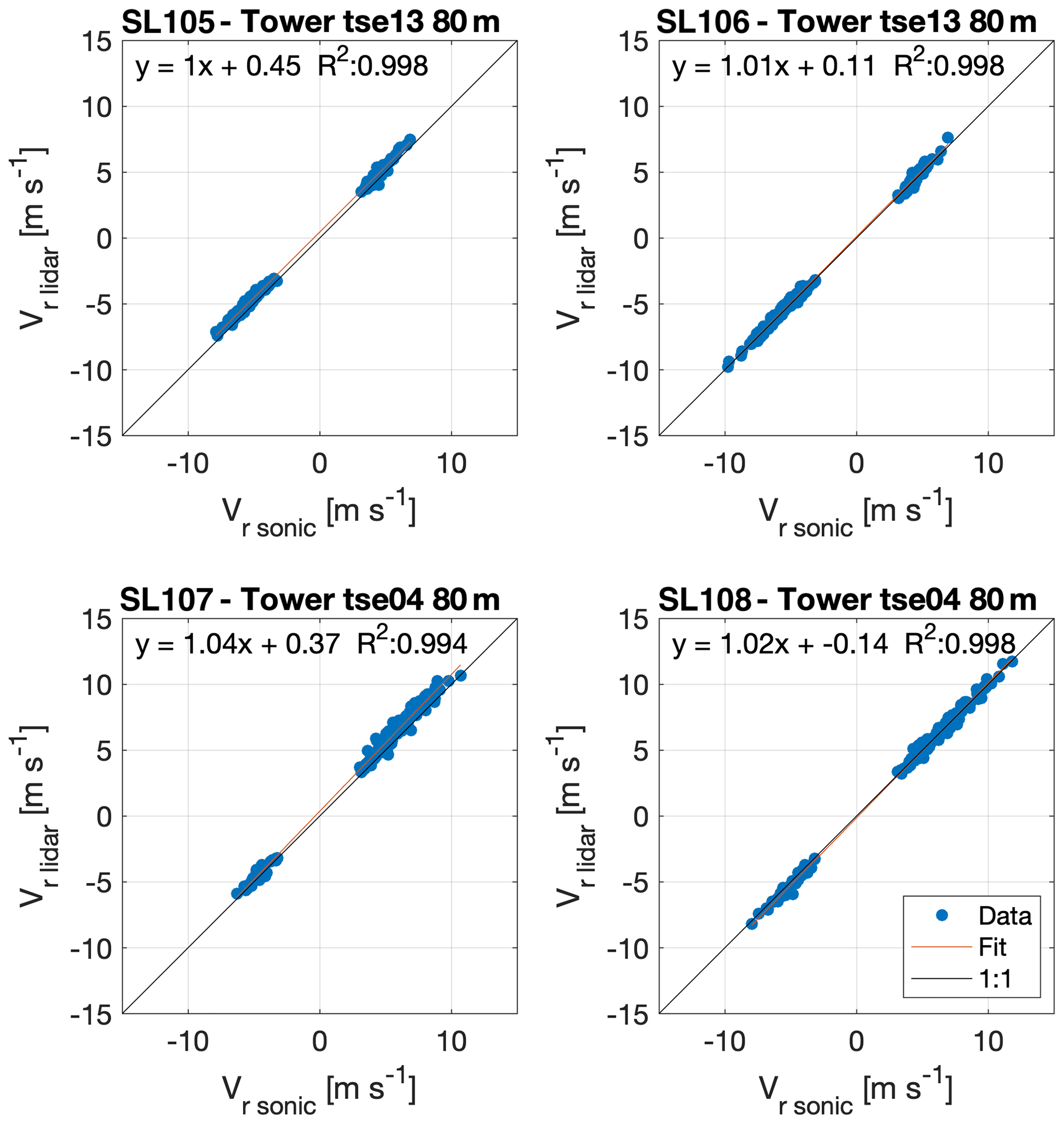
Figure 3Correlation of radial lidar wind speeds with the sonic wind speeds projected to the lidar LOSs. Only southwesterly and northeasterly wind directions are selected for sectors of ±15∘, centered around the transect and oriented 54∘ towards north.
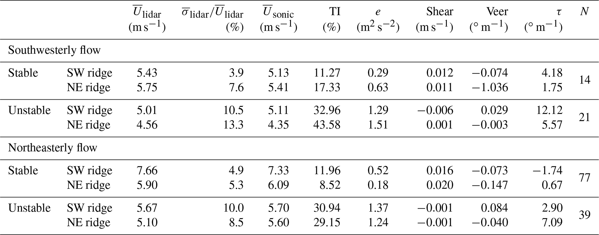
Table 3Observation from tower tse04 (SW ridge) and tse13 (NE ridge). Turbulence intensity is defined as , where is the mean wind speed and σU the standard deviation of Usonic. Turbulent kinetic energy is calculated as , where u′, v′, and w′ are the fluctuating parts of the wind vector components as measured by the sonic anemometers. Wind shear and veer are calculated over 60 m (40–100 m a.g.l.). The flow inclination angle τ is calculated as , where u and v are the mean horizontal wind vector components and w the vertical. All averages are taken over 10 min. is the mean of the wind speeds measured by the lidars averaged over the entire ridge. is the standard deviation also averaged along the ridge. N is the number of available 10 min periods.
5.1 Comparison of mast and lidar measurements
The correlation of radial velocities measured by the individual SLs and of the reconstructed wind vectors with the sonic wind speeds is calculated. For all SLs the correlation coefficient for the LOS measurements is better than 0.994, offsets are less than 0.45 m s−1, and slopes deviate by less than 0.04 from 1 (Fig. 3). Considering that the measurements are not collocated and that the measurement volumes of lidars and sonics differ by about 2 orders of magnitude, these correlations can be considered as good. For this comparison, only measurements from IOP are selected, and measurements are limited to the prevailing wind directions (±15∘, centered around the transect and oriented 54∘ towards north) to eliminate the effects of mast wind shadow and to be consistent with the data fraction used for the further analysis.
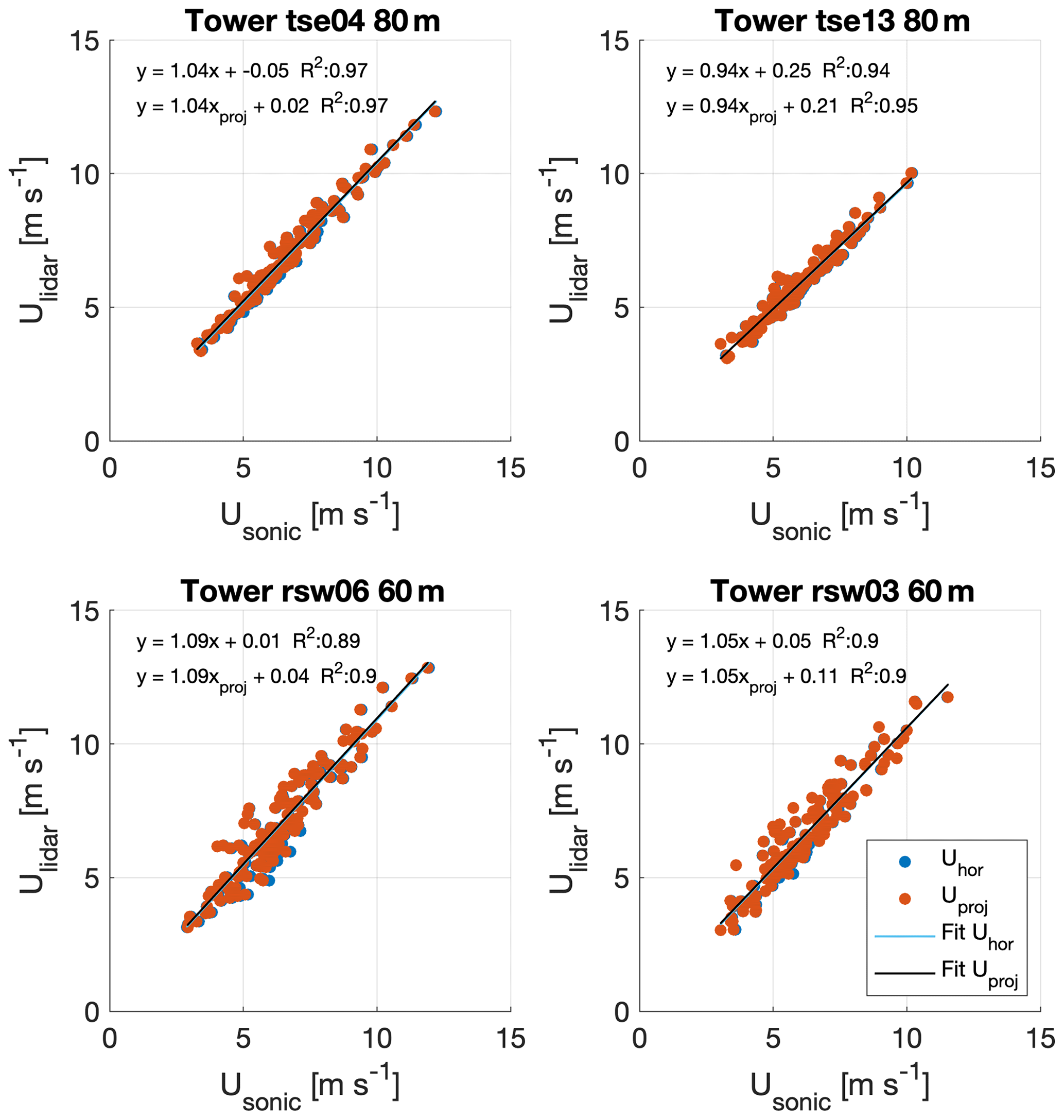
Figure 4Correlation of reconstructed lidar wind speeds with the horizontal sonic wind speeds and the sonic wind speeds projected to the plane spanned by the lidars. Only southwesterly and northeasterly wind directions are selected for sectors of ±15∘, centered around the transect and oriented 54∘ towards north. Wind speeds at tse04, rsw06, and rsw03 are derived from the SLs 107 and 108 and at tse13 from the SLs 105 and 106.
The correlation based on the reconstructed wind vectors is calculated for 10 min averages at all four masts for horizontal wind speeds and wind speeds projected to the plane spanned by the two lidar beams. Both correlation coefficients with the two 80 m sonics are better than 0.94, with offsets smaller than 0.25 m s−1 and slopes close to 1 (1.04 at tower tse04 and 0.94 at tower tse13; Fig. 4). At the 60 m masts the correlation of lidar and sonic measurements is lower due to the spatial difference in height. The correlation coefficients at both masts are 0.9.
Overall, the comparison aids the validation of the lidar measurements. However, the measurements cannot be compared to studies that were purely designed for a comparison of different measurement technologies as done, for example, by Pauscher et al. (2016). Moreover, the correlation of reconstructed wind speeds in the present study shows that differences when comparing the lidar wind speeds to the projected or the horizontal sonic winds speeds are negligibly small. This affirms that the decisions of using elevation angles below 5∘ is adequate to measure the horizontal wind with the present scanning trajectories.
5.2 Observed flow patterns
Considering all available ridge scan periods (507), we find that the mean wind speed is 10 % higher at the SW ridge. Relative changes in wind speed along the SW ridge are below 2 %. At the NE ridge, the lowest relative wind speeds are found at the terrain dip at 400 m, and a change of 7 % in mean wind speed is found along the ridge (not shown). This picture changes significantly during specific atmospheric conditions, which are analyzed in the following subsections. We segregate the data by the prevailing flow directions from the northeast and the southwest for sectors of ±15∘, centered perpendicular to the ridge and oriented at 54∘ (geographical convention). Furthermore, the data are segregated by the atmospheric stability characterized by the Richardson number (Ri).
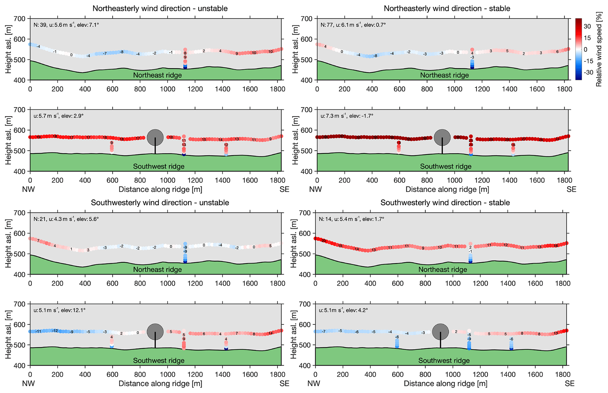
Figure 5Normalized wind speeds measured by the lidars and sonics during different atmospheric conditions. The wind speeds are normalized by the mean along the upstream ridge; e.g., for southwesterly wind directions all measurements are normalized with the mean wind speed along the SW ridge. N is the number of 10 min periods; u is the horizontal wind speed measured by the 80 m sonic anemometer; “elev” is the flow elevation angle measured by the 80 m sonic anemometer.
5.2.1 Dependence on wind direction
For southwesterly flows, an increase of more than 20 % in relative wind speeds is observed along the SW ridge, with higher wind speeds in the southeast and lower wind speeds in the northwest (Fig. 5). At the NE ridge, for southwesterly flow, increased relative wind speeds of up to 13 % are observed at the NW end of the ridge, where the elevation increases. All values are relative to the mean wind speed along the upstream ridge.
For northeasterly flow, significantly higher wind speeds of about 25 % are observed at the SW ridge. Additionally, a change in wind speed along the SW ridge is observed with higher speeds in the northwest and lower wind speeds in the southeast, which is opposite to the observation under southwesterly flow. For some conditions, the change in relative wind speed is higher than 20 %.
We considered these observations as statistically significant as the mean of standard deviations calculated at each point along the ridge is much lower than the observed changes (Table 3).
5.2.2 Dependence on atmospheric stability
It is most notable that wind speeds at the downwind ridge are always higher than at the upstream ridge during stable conditions (Fig. 5). The mean wind speeds along the downwind ridge measured by the lidars are 1.8 m s−1 higher during northeasterly flow and 0.3 m s−1 higher for southwesterly flows. Moreover, the mast measurements show consistently negative wind shear during stable conditions at both masts and, as expected, lower levels of turbulence intensity and turbulent kinetic energy (Table 3).
During unstable atmospheric conditions, wind speeds are higher at the SW ridge for both flow directions. The large flow inclination angles measured by the sonics at the upstream ridges of 12.12∘ (7.09∘) for SW flow (NE flow) are also remarkable. The much higher flow inclination angle for SW flow over the SW ridge supports the findings of Menke et al. (2018b) that the wind turbine wake is lifted higher during the day (unstable) than during the night (stable).
5.3 Comparison of lidar measurements and simulations
As described in Sect. 3, we compare the ridge scan measurements to the WRF-LESs with and without forest drag implementation. Data from both simulations are extracted at the coordinates of the ridge scan points and interpolated to the exact measurement periods in time.
The best agreement, considering all available ridge scan periods, is reached for the WRF_NF simulation without forest drag in terms of mean difference, root mean square error (RMSE), and bias. In this case, the WRF model overestimates the wind speeds by 6.5 % and 4.1 % at the SW ridge and NE ridge, respectively (see Table 4). The WRF_F simulation with forest drag implementation underestimates the wind speeds along the ridges by −35.2 % (−32.2 %) at the SW (NE) ridge. This underestimation of simulated wind speeds on the ridge tops was also observed by Wagner et al. (2019b) and is most likely caused by an overrepresentation of the forest drag due to incorrect forest coverage on the ridge tops and too high trees in the model. As described in Sect. 3, an average canopy height of 30 m was used, whereas real tree heights obtained from an aerial laser scan in 2015 were of the order of 15 m (see Fig. 1b). The distribution of forested areas in Fig. 1b further indicates that the ridge tops were mostly free of trees, whereas both ridge tops are forested in the model according to the CORINE land use data set (see Fig. 3 in Wagner et al., 2019b).
Table 4Mean difference of WRF simulations and ridge scans calculated as and averaged along the entire ridge. Correlation coefficient (COR) and root mean square error (RMSE) values for the comparison of WRF data with the ridge scan measurements. The first number states the value for the WRF_NF simulation without forest parameterization and the number in brackets the value for the WRF_F run with forest parameterization. Bold values indicate the best model per parameter. The percentage of lidar observations, which describe the respective flow condition, is indicated in the last column.
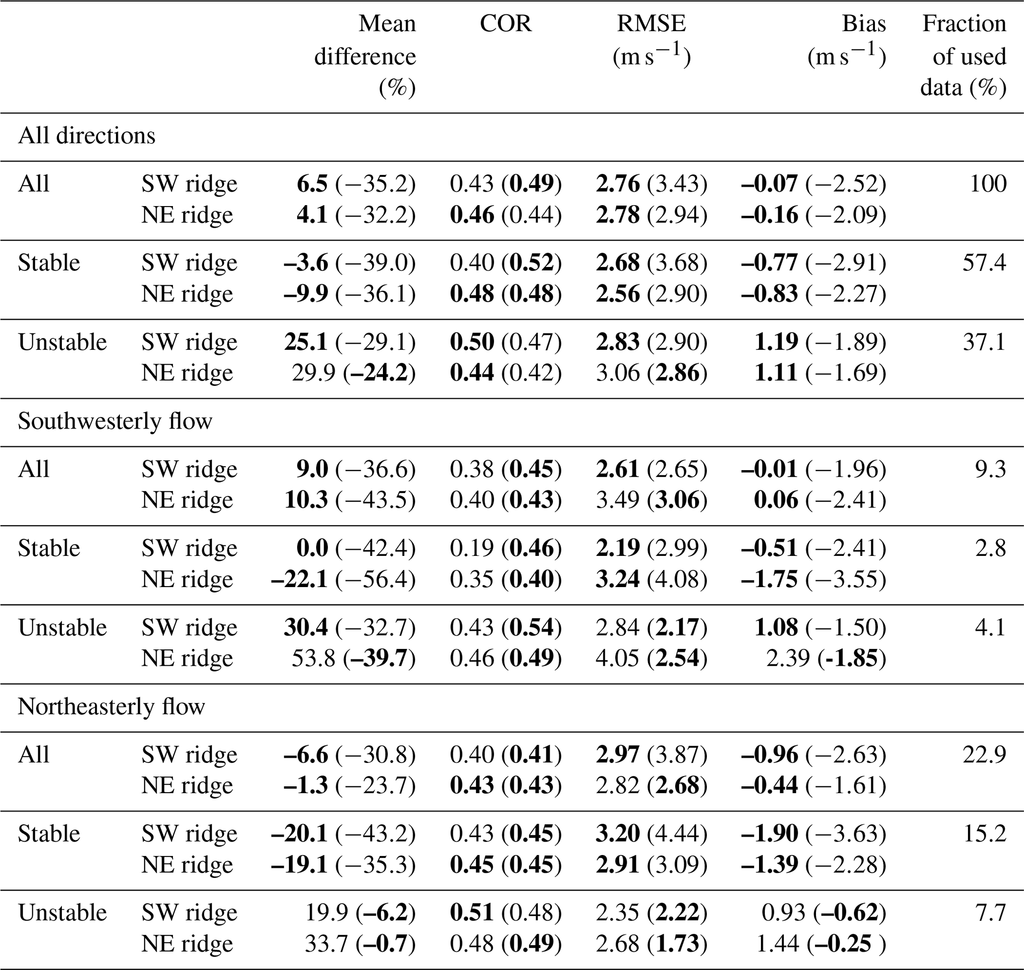
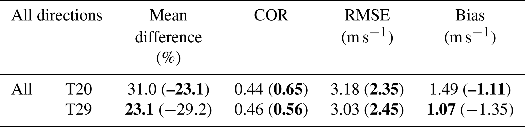
Even though the simulation with forest drag underestimates wind speeds at the ridges, it shows improved correlation with the measurements (see Table 4). Correlation coefficients are consistently better for southwesterly wind directions and better or similar to the correlations of the simulation without forest drag for northeasterly flow. A comparison of the same simulations with multiple meteorological masts across the double ridge along transect southeast (TSE; equal to transect 2 in Fernando et al., 2019) in Wagner et al. (2019b) shows a clear improvement of simulated wind speeds in the WRF_F simulation with forest parameterization. This means that the forest parameterization enhances the simulated flow, especially along the slopes of the ridges, where wind speeds are overestimated in the WRF_NF simulation. When comparing the simulations only to the two 100 m towers tse04 (T20) and tse13 (T29) on the SW and NE ridge, respectively, the WRF_F run underestimates wind speeds at 80 m a.g.l. but shows improved correlation values and RMSEs (see Table 5 in this paper and Table 4 in Wagner et al., 2019b). The better results for the WRF_F run for the comparison with tse04 and tse13 may be induced by the larger number of samples that are available in the tower data set (about 13 500 data points) compared to lidar data (507 points in time), representing a larger spectrum of different meteorological conditions.
Table 5As in Table 4 but for comparison of WRF simulations with tower T20 (tse04) and T29 (tse13) on the SW and NE ridge, respectively.
Segregating the data into different atmospheric conditions shows that the WRF_NF run performs best under stable atmospheric conditions (Table 4). For unstable conditions, the WRF_F simulation performs better at the NE ridge and for northeasterly wind also at the SW ridge. Considering that the flow is more turbulent under unstable conditions, it can be assumed that more mixing and interaction with the forest take place compared to stable conditions, during which the forest rather acts as a displacement. For northeasterly winds, the high forest density for the fetch upstream of the NE ridge (see Fig. 3 in Wagner et al., 2019b) might lead to better results of WRF with forest drag.
Figure 6 shows the spatial distribution of averaged wind speeds along the SW and NE ridges during southwesterly flow. The general underestimation of wind speeds in the WRF_F simulation is visible. Disregarding this negative offset, the WRF_F simulation shows spatial changes in wind speed along the ridges that are more similar to changes measured with the lidars compared to stronger gradients along the ridges in the WRF_NF simulation.
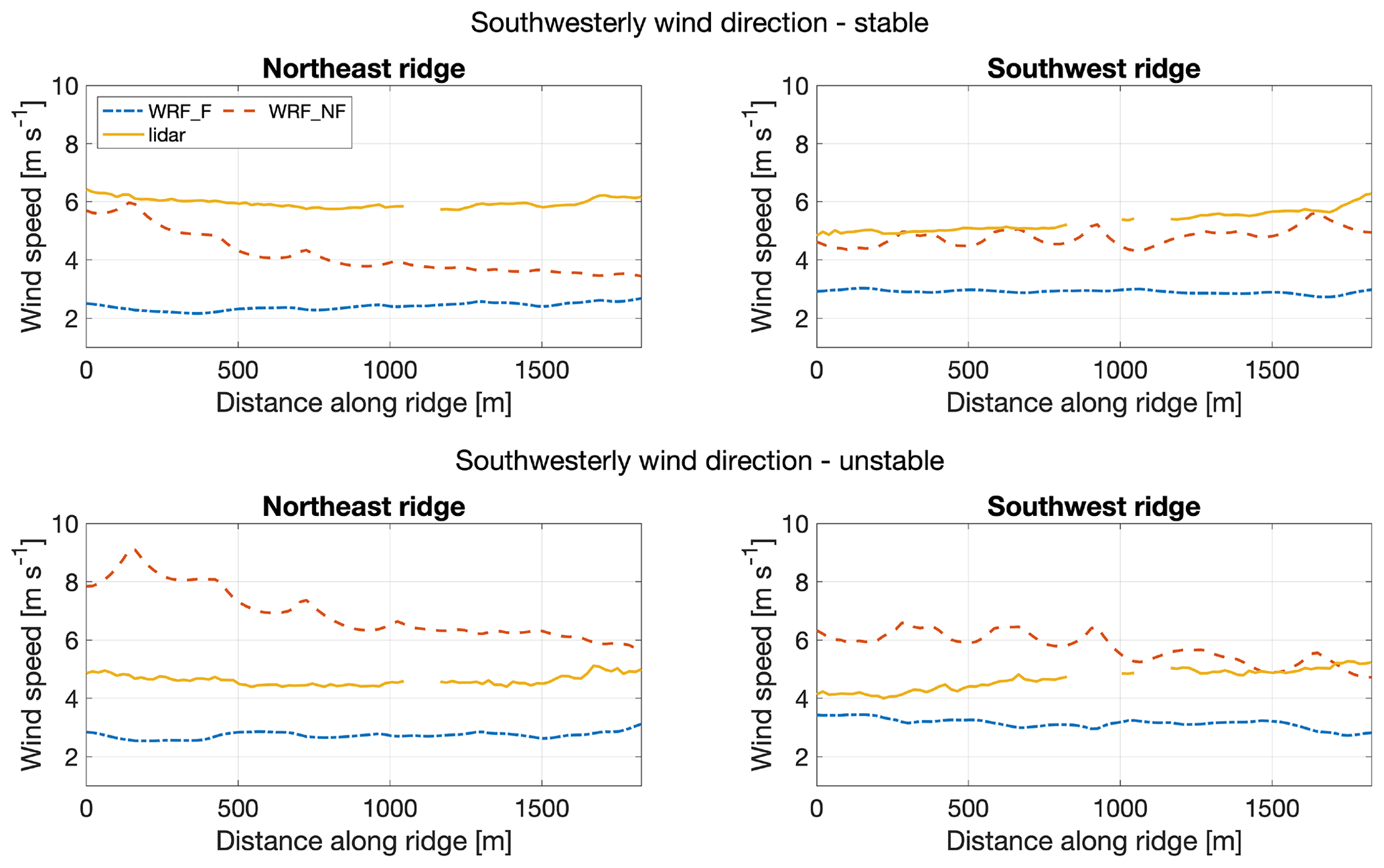
Figure 6Comparison of WRF wind speeds and lidar ridge scan measurements for southwesterly flow, segregated into stable and unstable conditions.
The results and observations outlined above demonstrate the ability of the SLs to perform flow measurements over large areas. The design of the scanning scenario allowed us to capture fine differences in the flow field along the two ridges at Perdigão. Here we want to discuss three of the observed flow characteristics. Firstly, we observed on average a slowdown of the flow at the terrain dip, which seems to be in accordance with the classical linear flow perturbation theory. Apparently, the influence of channeling effects, which are expected under stably stratified conditions as described by Vassallo et al. (2020), is not significant enough to affect the mean wind speed. The ratio of ridge height to dip height is most likely too large to cause channeling effects that have a significant influence on the mean flow field at a height of 80 m a.g.l., i.e., heights of interest for wind energy production.
Secondly, we want to focus the discussion on the wind speed changes along the SW ridge. The linear theory says that orography gives a speedup with the same magnitude for opposite wind directions. Accordingly, if orography is solely responsible for the speedup along the ridge, the trend would be the same whether the wind is from the southwest or northeast. As we observed the exact opposite (for SW wind directions flow speed is highest at the SE end of the SW ridge, and flow speeds are higher at the NW end for NE wind directions), we can conclude that orography is not solely responsible. It is likely that the trend observed along the SW ridge is an interaction of orography and roughness effects. For roughness, contrary to orography, the speedup along the ridge is only affected by the roughness (i.e., the friction drag) of the terrain upstream. This explains the lower wind speeds in the southeast of the SW ridge for NE winds as the density of larger trees increases to the southeast (Fig. 1b). For SW winds the higher wind speeds at the SE end are most likely caused by an increasing steepness of the terrain and a decreasing steepness of the terrain from the northwest towards the southeast (Fig. 1a and Fig. 2 in Menke et al., 2018b).
Lastly, we want to focus on the flow observations under stably stratified conditions. The higher wind speeds observed at the downstream ridges under these conditions as described in Sect. 5.2.2 are explainable by the speedup that is caused by the formation of atmospheric waves during stable conditions as shown in Palma et al. (2019) and Fernando et al. (2019, Fig. 7d).
The observations show that, as expected, the flow is as complex as the terrain. Thus, reproducing the flow conditions with simulations is challenging as shown by the comparison with WRF-LES results (Sect. 5.3). Summarizing, we find a high sensitivity of the WRF-LESs to the parameterization of surface friction. Adding a forest drag term significantly changes the results. The comparison of the simulations with the lidar ridge scans reveals that the forest drag is too strong on the ridge tops, which results in underestimated wind speeds. Without forest drag, wind speeds are overestimated on average. The comparison of the same simulations with multiple meteorological towers across the double ridge in Wagner et al. (2019b) shows an improvement of the simulated flow with forest parameterization. Furthermore, relative changes in wind speed along the ridges are more similar for the simulation with forest drag when comparing to the relative changes observed with the SLs. This shows that the forest parameterization has a positive effect on simulated wind speeds over Perdigão but makes clear that the horizontal distribution of forested areas and the tree heights have to be more realistic in future model setups. This will only be possible by using the high-resolution aerial laser scans used for the canopy height estimation in Fig. 1b or by introducing better land use data sets, which include seasonal variability of the canopy layer, e.g., caused by forestry and agriculture.
Flow over complex terrain causes challenges for wind energy projects. High spatial variability makes the selection of sites for wind turbines far from obvious. Capturing the spatial variability with measurements and flow simulation is generally challenging. At the measurement site, the spatial variability can be addressed by increasing the number of measurement locations. This can be done with scanning lidars as they can provide wind measurements over areas of several square kilometers. For simulating the flow, highly resolved advanced computer models are needed.
In our study, we present measurements of two pairs of SLs that were designed to assess the flow conditions at locations favorable for wind turbines during the Perdigão measurement campaign. The SLs retrieve the mean horizontal velocity profiles of 1.8 km in length along two ridges. We find a good correlation of the lidar measurements with sonic wind measurements at masts along ridges. Moreover, we show that using advanced lidar data filtering methods improves the measurement availability by 20 %. Our analysis of the flow fields along the ridges demonstrates the ability of the SLs to reveal significant details about the flow that would remain unrecognized when only few measurement locations are available.
The comparison of measurements and two WRF-LESs reveals a high sensitivity of the model to the parameterization of surface friction, causing significant deviations between measurements and the simulation. It is assumed that a wrong forest distribution in the model on the ridge tops and an overestimated tree height are the main reasons for the poor agreement of the simulation with additional forest parameterization. However, this study and Wagner et al. (2019b) show a considerably improved correlation of measurements and the simulation when the parameterization is used.
Overall, we conclude that SL measurements are a valuable tool to assess wind resources in complex terrain. They help to understand the flow conditions and to validate simulations which are still challenged by the complexity of the topography. In the future, the SL system availability, which was only at 44 % for the period investigated in this study, has to be improved. The main factors influencing the availability were software issues, hardware failures, and power outages. Moreover, we recommend basing flow simulations on as realistic as possible land use data, as for example acquired by Boudreault et al. (2015), and including seasonal variability of the canopy distribution.
The scanning lidar data for the entire measurement campaign are made available by Menke et al. (2018a). The measurement mast data are made available by NCAR for the 5 min averaged data (UCAR/NCAR – Earth Observing Laboratory, 2019b) and for high-resolution data (UCAR/NCAR – Earth Observing Laboratory, 2019a).
RM performed the analysis and wrote the main body of the manuscript. JW performed the WRF simulation and wrote Sect. 3. RM, JM, and NV designed the lidar part of the field campaign. All authors were involved in designing the methodology, took part in the writing and reviewing process, and contributed with critical feedback to this paper.
The authors declare that they have no conflict of interest.
This article is part of the special issue “Flow in complex terrain: the Perdigão campaigns (ACP/WES/AMT inter-journal SI)”. It does not belong to a conference.
We acknowledge the work of everyone involved in the planning and execution of the campaign. In specific we would like to thank Stephan Voß, Julian Hieronimus (ForWind, University of Oldenburg), Per Hansen, and Preben Aagaard (DTU Wind Energy) for their help with the installation of the scanning lidars. We are also grateful for the contribution of three scanning lidars to the campaign by ForWind. Moreover, without the intensive negotiations of José Carlos Matos (INEGI) with local landowners about specific locations for our scanning lidars, this research would not be possible. We are grateful to the municipality of Vila Velha de Ródão; the landowners who authorized installation of scientific equipment on their properties; the residents of Vale do Cobrão, Foz do Cobrão, Alvaiade, and Chão das Servas; and the local businesses who kindly contributed to the success of the campaign. The space for the operational center was generously provided by Centro Sócio-Cultural e Recreativo de Alvaiade in Vila Velha de Ródão.
We thank the Danish Energy Agency for funding through the New European Wind Atlas project (EUDP 14-II). The contribution of Robert Menke is partly based upon work supported by the National Center for Atmospheric Research, which is a major facility sponsored by the National Science Foundation under cooperative agreement no. 1852977. Any opinions, findings and conclusions, or recommendations expressed in this material do not necessarily reflect the views of the National Science Foundation.
This paper was edited by Sandrine Aubrun and reviewed by two anonymous referees.
Bechmann, A., Sørensen, N. N., Berg, J., Mann, J., and Réthoré, P.-E.: The Bolund Experiment, Part II: Blind Comparison of Microscale Flow Models, Bound.-Lay. Meteorol., 141, 245, https://doi.org/10.1007/s10546-011-9637-x, 2011. a
Beck, H. and Kühn, M.: Dynamic Data Filtering of Long-Range Doppler LiDAR Wind Speed Measurements, Remote Sens.-Basel, 9, 561, https://doi.org/10.3390/rs9060561, 2017. a
Berg, J., Troldborg, N., Menke, R., Patton, E. G., Sullivan, P. P., Mann, J., and Sørensen, N.: Flow in complex terrain – a Large Eddy Simulation comparison study, J. Phys. Conf. Ser., 1037, 072015, https://doi.org/10.1088/1742-6596/1037/7/072015, 2018. a
Bingöl, F., Mann, J., and Foussekis, D.: Conically scanning lidar error in complex terrain, Meteorol. Z., 18, 189–195, https://doi.org/10.1127/0941-2948/2009/0368, 2009. a
Bodini, N., Zardi, D., and Lundquist, J. K.: Three-dimensional structure of wind turbine wakes as measured by scanning lidar, Atmos. Meas. Tech., 10, 2881–2896, https://doi.org/10.5194/amt-10-2881-2017, 2017. a
Boudreault, L.-É., Bechmann, A., Tarvainen, L., Klemedtsson, L., Shendryk, I., and Dellwik, E.: A LiDAR method of canopy structure retrieval for wind modeling of heterogeneous forests, Agr. Forest Meteorol., 201, 86–97, https://doi.org/10.1016/j.agrformet.2014.10.014, 2015. a
Clifton, A., Clive, P., Gottschall, J., Schlipf, D., Simley, E., Simmons, L., Stein, D., Trabucchi, D., Vasiljevic, N., and Würth, I.: IEA Wind Task 32: Wind lidar identifying and mitigating barriers to the adoption of wind lidar, Remote Sens.-Basel, 10, 406, https://doi.org/10.3390/rs10030406, 2018. a
Daniels, M. H., Lundquist, K. A., Mirocha, J. D., Wiersema, D. J., and Chow, F. K.: A new vertical grid nesting capability in the Weather Research and Forecasting (WRF) Model, Mon. Weather Rev., 144, 3725–3747, https://doi.org/10.1175/MWR-D-16-0049.1, 2016. a
Fernando, H., Mann, J., Palma, J., Lundquist, J., Barthelmie, R., BeloPereira, M., Brown, W., Chow, F., Gerz, T., Hocut, C., Klein, P., Leo, L., Matos, J., Oncley, S., Pryor, S., Bariteau, L., Bell, T., Bodini, N., Carney, M., Courtney, M., Creegan, E., Dimitrova, R., Gomes, S., Hagen, M., Hyde, J., Kigle, S., Krishnamurthy, R., Lopes, J., Mazzaro, L., Neher, J., Menke, R., Murphy, P., Oswald, L., Otarola-Bustos, S., Pattantyus, A., Rodrigues, C. V., Schady, A., Sirin, N., Spuler, S., Svensson, E., Tomaszewski, J., Turner, D., van Veen, L., Vasiljević, N., Vassallo, D., Voss, S., Wildmann, N., and Wang, Y.: The Perdigão: Peering into Microscale Details of Mountain Winds, B. Am. Meteorol. Soc., 100, 799–819, https://doi.org/10.1175/BAMS-D-17-0227.1, 2019. a, b, c, d
Iungo, G. V., Wu, Y.-T., and Porté-Agel, F.: Field Measurements of Wind Turbine Wakes with Lidars, J. Atmos. Ocean. Tech., 30, 274–287, https://doi.org/10.1175/JTECH-D-12-00051.1, 2013. a
Klemp, J., Dudhia, J., and Hassiotis, A.: An upper gravity-wave absorbing layer for NWP applications, Mon. Weather Rev., 136, 3987–4004, https://doi.org/10.1175/2008MWR2596.1, 2008. a
Lange, J., Mann, J., Angelou, N., Berg, J., Sjöholm, M., and Mikkelsen, T.: Variations of the Wake Height over the Bolund Escarpment Measured by a Scanning Lidar, Bound.-Lay. Meteorol., 159, 147–159, https://doi.org/10.1007/s10546-015-0107-8, 2016. a
Lange, J., Mann, J., Berg, J., Parvu, D., Kilpatrick, R., Costache, A., Chowdhury, J., Siddiqui, K., and Hangan, H.: For wind turbines in complex terrain, the devil is in the detail, Environ. Res. Lett., 12, 094020, https://doi.org/10.1088/1748-9326/aa81db, 2017. a
Mann, J., Angelou, N., Arnqvist, J., Callies, D., Cantero, E., Arroyo, R. C., Courtney, M., Cuxart, J., Dellwik, E., Gottschall, J., Ivanell, S., Kühn, P., Lea, G., Matos, J. C., Palma, J. M. L. M., Pauscher, L., Peña, A., Rodrigo, J. S., Söderberg, S., Vasiljevic, N., and Rodrigues, C. V.: Complex terrain experiments in the New European Wind Atlas, Philos. T. Roy. Soc. A, 375, 20160101, https://doi.org/10.1098/rsta.2016.0101, 2017. a
Mann, J., Peña, A., Troldborg, N., and Andersen, S. J.: How does turbulence change approaching a rotor?, Wind Energ. Sci., 3, 293–300, https://doi.org/10.5194/wes-3-293-2018, 2018. a
Menke, R., Mann, J., and Vasiljevic, N.: Perdigão-2017: multi-lidar flow mapping over the complex terrain site, Technical University of Denmark, https://doi.org/10.11583/DTU.7228544.v1, 2018a. a
Menke, R., Vasiljević, N., Hansen, K. S., Hahmann, A. N., and Mann, J.: Does the wind turbine wake follow the topography? A multi-lidar study in complex terrain, Wind Energ. Sci., 3, 681–691, https://doi.org/10.5194/wes-3-681-2018, 2018b. a, b, c
Menke, R., Mann, J., and Svensson, E.: Perdigão 2017: GPS survey of sonic anemometers and WindScanners operated by DTU, DTU Wind Energy, Denmark, 2019a. a
Menke, R., Vasiljević, N., Mann, J., and Lundquist, J. K.: Characterization of flow recirculation zones at the Perdigão site using multi-lidar measurements, Atmos. Chem. Phys., 19, 2713–2723, https://doi.org/10.5194/acp-19-2713-2019, 2019b. a
Mikkelsen, T., Angelou, N., Hansen, K., Sjöholm, M., Harris, M., Slinger, C., Hadley, P., Scullion, R., Ellis, G., and Vives, G.: A spinner-integrated wind lidar for enhanced wind turbine control, Wind Energy, 16, 625–643, https://doi.org/10.1002/we.1564, 2013. a
Palma, J., Lopes, A. S., Gomes, V. C., Rodrigues, C. V., Menke, R., Vasiljević, N., and Mann, J.: Unravelling the wind flow over highly complex regions through computational modeling and two-dimensional lidar scanning, J. Phys. Conf. Ser., 1222, 012006, https://doi.org/10.1088/1742-6596/1222/1/012006, 2019. a, b, c
Pauscher, L., Vasiljevic, N., Callies, D., Lea, G., Mann, J., Klaas, T., Hieronimus, J., Gottschall, J., Schwesig, A., Kühn, M., and Courtney, M.: An Inter-Comparison Study of Multi- and DBS Lidar Measurements in Complex Terrain, Remote Sens.-Basel, 8, 782, https://doi.org/10.3390/rs8090782, 2016. a, b
Pineda, N., Jorba, O., Jorge, J., and Baldasano, J. M.: Using NOAA AVHRR and SPOT VGT data to estimate surface parameters: application to a mesoscale meteorological model, Int. J. Remote Sens., 25, 129–143, https://doi.org/10.1080/0143116031000115201, 2004. a
Sathe, A. and Mann, J.: A review of turbulence measurements using ground-based wind lidars, Atmos. Meas. Tech., 6, 3147–3167, https://doi.org/10.5194/amt-6-3147-2013, 2013. a
Shaw, T. H. and Schumann, U.: Large-eddy simulation of turbulent flow above and within a forest, Bound.-Lay. Meteorol., 61, 47–64, https://doi.org/10.1007/BF02033994, 1992. a
Simley, E., Angelou, N., Mikkelsen, T., Sjöholm, M., Mann, J., and Pao, L. Y.: Characterization of wind velocities in the upstream induction zone of a wind turbine using scanning continuous-wave lidars, J. Renew. Sustain. Energ., 8, 013301, https://doi.org/10.1063/1.4940025, 2016. a
Skamarock, W. C., Klemp, J. B., Dudhia, J., Gill, D. O., Barker, D. M., Duda, M. G., Huang, X.-Y., Wang, W., and Powers, J. G.: A description of the Advanced Research WRF Version 3, NCAR technical note, Mesoscale and Microscale Meteorology Division, National Center for Atmospheric Research, Boulder, Colorado, USA, available at: https://www2.mmm.ucar.edu/wrf/users/docs/arw_v3_bw.pdf (last access: 2 August 2020), 2008. a
Trujillo, J.-J., Bingöl, F., Larsen, G. C., Mann, J., and Kühn, M.: Light detection and ranging measurements of wake dynamics. Part II: two-dimensional scanning, Wind Energy, 14, 61–75, https://doi.org/10.1002/we.402, 2011. a
UCAR/NCAR – Earth Observing Laboratory: NCAR/EOL Quality Controlled High-rate ISFS surface flux data, geographic coordinate, tilt corrected, Version 1.1, UCAR/NCAR – Earth Observing Laboratory, https://doi.org/10.26023/8x1n-tct4-p50x, 2019a. a
UCAR/NCAR – Earth Observing Laboratory: NCAR/EOL Quality Controlled 5-minute ISFS surface flux data, geographic coordinate, tilt corrected, Version 1.1, UCAR/NCAR – Earth Observing Laboratory, https://doi.org/10.26023/zdmj-d1ty-fg14, 2019b. a
Vasiljević, N.: A time-space synchronization of coherent Doppler scanning lidars for 3D measurements of wind fields, PhD thesis, DTU Wind Energy, Denmark, 2014. a
Vasiljević, N., Lea, G., Courtney, M., Cariou, J.-P., Mann, J., and Mikkelsen, T.: Long-range WindScanner system, Remote Sens.-Basel, 8, 896, https://doi.org/10.3390/rs8110896, 2016. a, b
Vasiljević, N., L. M. Palma, J. M., Angelou, N., Carlos Matos, J., Menke, R., Lea, G., Mann, J., Courtney, M., Frölen Ribeiro, L., and M. G. C. Gomes, V. M.: Perdigão 2015: methodology for atmospheric multi-Doppler lidar experiments, Atmos. Meas. Tech., 10, 3463–3483, https://doi.org/10.5194/amt-10-3463-2017, 2017. a, b, c
Vasiljević, N., Vignaroli, A., Bechmann, A., and Wagner, R.: Digitalization of scanning lidar measurement campaign planning, Wind Energ. Sci., 5, 73–87, https://doi.org/10.5194/wes-5-73-2020, 2020. a
Vassallo, D., Krishnamurthy, R., Menke, R., and Fernando, H. J.: Observations of stably stratified flow through a microscale gap, J. Atmos. Sci., in review, 2020. a
Wagner, J., Gerz, T., Wildmann, N., and Gramitzky, K.: Long-term simulation of the boundary layer flow over the double-ridge site during the Perdigão 2017 field campaign, Atmos. Chem. Phys., 19, 1129–1146, https://doi.org/10.5194/acp-19-1129-2019, 2019a. a, b, c, d
Wagner, J., Wildmann, N., and Gerz, T.: Improving boundary layer flow simulations over complex terrain by applying a forest parameterization in WRF, Wind Energ. Sci. Discuss., https://doi.org/10.5194/wes-2019-77, 2019b. a, b, c, d, e, f, g, h, i, j, k