US East Coast synthetic aperture radar wind atlas for offshore wind energy

We present the first synthetic aperture radar (SAR) offshore wind atlas of the US East Coast from Georgia to the Canadian border. Images from RADARSAT-1, Envisat, and Sentinel-1A/B are processed to wind maps using the geophysical model function (GMF) CMOD5.N. Extensive comparisons with 6008 collocated buoy observations of the wind speed reveal that biases of the individual systems range from −0.8 to 0.6 m s⁻¹. Unbiased wind retrievals are crucial for producing an accurate wind atlas, and intercalibration of the SAR observations is therefore applied. Wind retrievals from the intercalibrated SAR observations show biases in the range of to −0.2 to 0.0 m s⁻¹, while at the same time improving the root-mean-squared error from 1.67 to 1.46 m s⁻¹. The intercalibrated SAR observations are, for the first time, aggregated to create a wind atlas at the height 10 m a.s.l. (above sea level). The SAR wind atlas is used as a reference to study wind resources derived from the Wind Integration National Dataset Toolkit (WTK), which is based on 7 years of modelling output from the Weather Research and Forecasting (WRF) model. Comparisons focus on the spatial variation in wind resources and show that model outputs lead to lower coastal wind speed gradients than those derived from SAR. Areas designated for offshore wind development by the Bureau of Ocean Energy Management are investigated in more detail; the wind resources in terms of the mean wind speed show spatial variations within each designated area between 0.3 and 0.5 m s⁻¹ for SAR and less than 0.2 m s⁻¹ for the WTK. Our findings indicate that wind speed gradients and variations might be underestimated in mesoscale model outputs along the US East Coast.

1 Introduction

Offshore wind energy has been established on the continental shelf of northern Europe since 2001 with a total installed capacity of 15 780 MW (Wind Europe, 2018). The US East Coast is similar in water depths and population density and could thus be well-suited for offshore wind farms (Kempton et al., 2007). During the past decade, the Bureau of Offshore Energy Management (BOEM) has leased out areas designated for offshore wind farm development along the US East Coast (BOEM, 2018), and the first wind plant became operational in 2016 (Block Island Wind Farm, Rhode Island¹). Accurate and long-term wind statistics across broad geographic areas (i.e. wind atlases) are needed to support offshore wind energy deployment. Wind atlases can be developed from local in situ measurements, i.e. buoys or meteorological masts (Troen and Petersen, 1989); numerical weather prediction models; (Dvorak et al., 2013; Hahmann et al., 2015); or satellite-based remote sensing (Christiansen et al., 2006; Hasager et al., 2015).

Offshore wind resource data for the US East Coast are available from the Weather Research and Forecasting (WRF) model (Draxl et al., 2015b; Dvorak et al., 2013). For offshore wind energy, locations close to shore are most attractive because installation costs increase with the distance from shore because of increased water depth and longer cables. The BOEM lease areas are mainly located in coastal waters less than 70 km from shore where influences from upstream land masses are still substantial (Barthelmie et al., 2007), and mesoscale models can result in high uncertainties (Hahmann et al., 2015). These models need validation. Colle et al. (2016) point out that observations at turbine hub heights around 100 m are lacking and provide case-study-based validation using observations from aeroplanes. Long-term reference wind climates at broad geospatial scales are missing because observations from ocean buoys are sparse.

Scatterometers and synthetic aperture radar (SAR) on board satellites provide coverage over several hundred kilometres, and it is possible to retrieve wind speeds at 10 m from radar backscatter of the ocean surface. SAR is better suited for resolving winds in coastal zones because of its higher spatial resolution (Christiansen et al., 2006). It has been shown that SAR-derived winds can accurately depict wind speed gradients measured by ground-based lidars near the coastline (Ahsbahs et al., 2017) and that SAR wind fields show similar mean wind speed variations as those experienced by wind turbines (Ahsbahs et al., 2018).

Wind resources can be assessed from SAR (Christiansen et al., 2006) and studies have been performed at different locations (Doubrawa et al., 2015; Hasager et al., 2011). For the US East Coast, a SAR-based wind atlas has been created from RADARSAT-1 (RS1) data for a small area off the coast of Delaware (Monaldo et al., 2014). Expanding this study to the entire US East Coast with RS1 data is not possible because the images were acquired specifically for this atlas and coverage outside this region is limited. Here, we have collected additional data from Envisat (ENV), Sentinel-1A (S1A), and Sentinel-1B (S1B), which are distributed via Copernicus services. These data are openly available to public research, which is not the case for data from other SAR missions such as TerraSAR-X, Cosmo SkyMed, or RADARSAT-2.

The objective of this study is to create and validate a satellite-based offshore wind atlas for the US East Coast and compare it to outputs from numerical weather prediction models.

The objective of this article is to produce and validate a SAR-based wind atlas for the US East Coast by merging observations from four different satellites. We will remove possible offsets between wind retrievals from the different SAR sensors and validate the intercalibrated dataset through comparisons with observations from the well-established ocean buoy network on the US East Coast. The SAR-based wind atlas will be compared to data from the Wind Integration National Dataset Toolkit (WTK) produced by the National Renewable Energy Laboratory (NREL) from 7 model years of outputs from the Weather Research and Forecasting (WRF) model (Draxl et al., 2015b). The WTK is a state-of-the-art mesoscale model run with a specific focus on parameters important for wind energy production. We focus on coastal wind speed gradients and determine how they are represented in wind atlases from SAR and WTK. Lastly, the spatial variation in mean wind speeds on the kilometre scale is investigated for BOEM lease areas designated for wind farm development.

The article is structured as follows: Sect. 2 provides an overview of the data and the area of interest for this study. Section 3 describes the methods used to create a SAR-based wind atlas. Section 4 presents wind climatologies and measurement artefacts of the SAR wind atlas. Section 5 focuses on using the SAR wind atlas to investigate wind variations and compares to the WTK. Section 6 contains a discussion of the results, and in Sect. 7, we draw conclusions on the potential use of the wind atlas.

2 Data and area of interest

2.1 Area of interest

We focus this study on coastal waters off the US East Coast from Georgia to the Canadian border. The area of interest is defined as between 30.7 and 45^∘ latitude and −63 and −81.3^∘ longitude extending 400 km offshore, as shown in Fig. 1. The positions of ocean buoys within the area are shown as well (see also Sect. 2.3).

Figure 1 Area of interest for this study and ocean buoy positions from the National Data Buoy Center.

2.2 Synthetic aperture radar

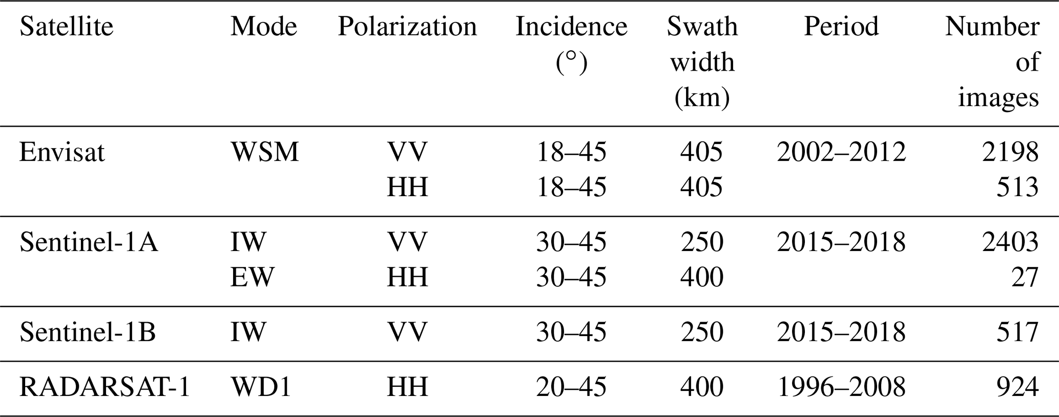
Satellites carrying SAR instruments have been operational for decades, and extensive image archives exist. Portions of these archives can be used by the scientific community, and the European Space Agency (ESA) archives are becoming increasingly open via Copernicus² services. SAR sensors usually operate in different modes depending on the desired spatial resolution of the images. We focus on modes that offer the widest possible swaths, because our aim is to create broad-scale wind resource maps. Co-polarized images in VV and HH modes from Envisat's wide swath mode (WSM), Sentinel-1's extra wide (EW) and interferometric wide (IW) modes, and RADARSAT-1's ScanSAR wide (WD1) mode are used throughout this study (Table 1). The number of images can be misleading when assessing the coverage of each sensor, because of the length of the swath varies. Envisat images tend to be more than 10 times longer than Sentinel-1 images. Sentinel-1A and B are operational at the moment, and data until May 2018 are included.

Table 1 Overview of SAR sensors and the respective imaging modes and properties. The period of operation and number of images included in this study are also shown.

2.3 Buoy data

High-quality wind and temperature measurements are available on the US East Coast from the buoy centre of the National Oceanic and Atmospheric Administration (NOAA) (National Data Buoy Center, 1971). Wind measurements at the buoy stations are obtained at various heights between 2 and 7 m a.s.l. (above sea level). The buoy observations are used here as reference measurements. We only use buoys located more than 5 km from the shoreline to avoid possible land contaminations in the corresponding SAR images. A total of 31 buoys fulfil this criterion, and their approximate locations are shown in Fig. 1. The majority of the buoys are located within 100 km from the shoreline. Locations and measurement heights are recorded annually in the buoy data files, but changes can occur within a year. Additional metadata on buoy positions and measurement heights are available and represent the most accurate information according to NOAA (National Data Buoy Center, 2015). We use the information given in the metadata. Buoy wind speeds and directions are measured every hour for 8 min, and data are automatically quality controlled (National Data Buoy Center, 2009). We perform additional quality control through manual inspection of data points where the difference between SAR and buoy wind speeds exceeds 10 m s⁻¹. This leads to removal of four periods from specific buoys that show unrealistically low wind speeds for several months and one short period where the buoy measurements are unreasonably high.

2.4 WIND toolkit

The WTK was originally developed to support the next generation of wind integration studies with input from experts at NREL in production cost modelling and atmospheric science. In its core lies a large dataset calculated with the WRF model. The WRF model version 3.4.1 was used to create the meteorological dataset, using ERA-Interim reanalysis data as inputs. The meteorological dataset has a spatial resolution of 2 km × 2 km and 5 min temporal resolution. It covers 7 years (2007–2013) and is available over the 48 contiguous US states, including the outer continental shelf. The WTK has been used by various research centres within NREL and by universities in multiple studies. A validation report is available for six onshore sites and three offshore sites (Draxl et al., 2015a). We will use the abbreviation WTK throughout this paper when referring to this particular dataset.

3 Methods

3.1 Synthetic aperture radar wind retrievals

SAR wind retrievals from the database of the Technical University of Denmark are used for this study and their processing is described in the following. SAR images are measures of the radar backscatter from the Earth's surface. The intensity of this backscatter is commonly referred to as the normalized radar cross section (NRCS). Level-1 SAR data are downloaded from the data providers, and calibration is applied to obtain the NRCS. The processing is done using the SAR Ocean Products System (SAROPS) software package (Monaldo et al., 2014). Radar backscatter and thus the NRCS of the ocean surface are determined by Bragg scattering (Valenzuela, 1978). This scattering mechanism is most sensitive to wave lengths on the order of 10 cm. At this scale, waves can be assumed to be in local equilibrium with the wind speed, and therefore the NRCS and the wind speed are correlated. An empirical geophysical model function (GMF) can link the NRCS and additional radar parameters to the wind speed at 10 m height above the sea surface.

For C-band radars, the C-band model (CMOD) family of functions is most widely used, and CMOD5.N (Hersbach, 2010) is chosen here for SAR wind retrievals. The retrieved wind speed is the equivalent neutral wind at 10 m above the sea surface. CMOD5.N is tuned for co-polarized vertical (VV) SAR observations, and an incidence-angle-dependent polarization ratio is applied before processing co-polarized horizontal (HH) images (Mouche et al., 2005). For SAR wind retrievals, the wind direction needs to be known a priori. Wind directions are taken from global weather models from 10 m wind vectors and are interpolated spatially to match the SAR images. Two sources of wind directions are used for the SAR wind retrieval: until 2010, wind directions come from the National Center for Atmospheric Research Climate Forecast System Reanalysis (CFSR) reanalysis data, and from 2011 onwards, wind directions from the Global Forecast System (GFS) are used. The switch in wind direction input is present in the database of derived SAR wind maps due to a change to near-real-time processing.

RADARSAT-1 was one of the early operational SAR systems, and some of the images have problematic distortions (Vachon et al., 1999), i.e. when stitching the subswaths together or there are issues with the geolocation. These typically cause overestimated NRCS values and thus wind speeds that are too high. Because these problems are easy to detect visually but hard to formalize, RADARSAT-1 data have been visually checked, and problematic images are excluded. Additionally, NRCS values above 44^∘ incidence angle are removed because of frequent unrealistically high NRCS values.

3.2 Merging synthetic aperture radar wind fields from different sensors

SAR wind speeds should correctly represent the wind conditions compared to in situ observations, but validation of SAR-derived wind speeds routinely leads to biases that are not consistent between studies (Christiansen et al., 2006; Horstmann et al., 2002; Lu et al., 2018; Takeyama et al., 2013). Deviations between studies can partially be explained by different GMFs that are used but also by inconsistent calibration of the NRCS. Biases in the SAR wind speeds are problematic here because they translate to biases in the derived wind atlas. It is particularly problematic to have offsets in the biases between sensors, because these will introduce variability where spatial coverage of sensors changes over the study area. To date, SAR wind atlases have used a singular sensor, or – if multiple sensors were merged – inherent differences have not been taken into account (Hasager et al., 2015; Karagali et al., 2018).

Badger et al. (2019) found systematic differences in the bias when comparing wind speeds retrieved from Envisat and Sentinel-1A/B against in situ observations. Biases for Envisat showed a strong incidence angle dependency and a bias drift over the sensor's lifetime. Badger et al. (2019) found that these biases can be corrected through a calculation of NRCS from the modelled winds that are used for the SAR wind inversion (see Sect. 2.4) followed by a comparison to the observed NRCS from the SAR. A linear fit of the NRCS differences depending on the incidence angle is then subtracted from the SAR observations before retrieving the SAR wind speeds. We apply the reported correction factors for Envisat and Sentinel-1A/B, which also account for the initial calibration problems of Sentinel-1A before 25 November 2015 (Miranda, 2015). Sentinel-1A data are split into two periods: before calibration (BC) and after calibration (AC). Corrections for RADARSAT-1 are not available in Badger et al. (2019), and, therefore, we calculate adjustment factors from the available RADARSAT-1 data using the same methodology. In accordance with recommendations from Badger et al. (2019), we exclude Envisat data acquired at incidence angles below 20^∘ because of increased scatter and bias in the adjustment method.

Synthetic aperture radar and buoy comparisons

Comparisons between SAR and buoy measurements are conducted to confirm whether results found in Badger et al. (2019) for northern Europe are consistently present in this dataset from the United States and whether the suggested adjustment method can remove biases between the sensors. Images during three storms with SAR wind speeds exceeding 30 m s⁻¹ have been removed from the comparison because co-polarized SAR wind retrievals are expected to perform poorly in these conditions.

Comparisons between the wind speed from buoys and SAR need to account for inherent differences in the measurements. SAR images are matched with the closest buoy time stamp with a maximum difference of 30 min (Monaldo, 1988). SAR winds are instantaneous, and they are averaged spatially to a 3 km by 3 km cell to better match the temporal average of buoy measurements. Anemometers on buoys are typically mounted at heights between 3 and 7 m while SAR winds are tuned to the height 10 m above the sea surface. Buoy wind speeds are therefore extrapolated to 1 m equivalent neutral winds using the Coupled Ocean–Atmosphere Experiment COARE 3.0 algorithm using temperature measurements from the buoys (Fairall et al., 2003). In this algorithm, atmospheric stratification is described using the difference between the air and sea temperature together with empirically found constants. The wind speed is then extrapolated considering atmospheric stability and roughness as described by Charnock's relation (Charnock, 1955).

Figure 2 shows comparisons between SAR and buoys as scatter plots for SAR winds processed as described in Sect. 3.1. We call this “default” processing as no inter-calibration of the SAR sensors is performed prior to wind retrieval processing. SAR wind speeds are split into 1 m s⁻¹ bins according to the buoy wind speed. The SAR mean wind speed and standard deviation around this mean are calculated and plotted as well. Comparisons for all collocations in Fig. 2a show a slight bias for SAR to overestimate wind speeds by 0.30 m s⁻¹. The RMSE of 1.67 m s⁻¹ is within the targets for satellite wind speed accuracies of 2 m s⁻¹ (Figa-Saldaña et al., 2002). Distinguishing between sensors shows that biases vary. Large biases towards overestimation of 0.62 and 0.82 m s⁻¹ are respectively found in Envisat (Fig. 2b) and Sentinel-1A BC (Fig. 2e), while RADARSAT-1 (Fig. 2c) underestimates wind speeds by 0.89 m s⁻¹. Both Sentinel-1A AC (Fig. 2f) and Sentinel-1B (Fig. 2d) have neglectable biases. The results for Envisat and the two Sentinels are in line with findings in Badger et al. (2019).

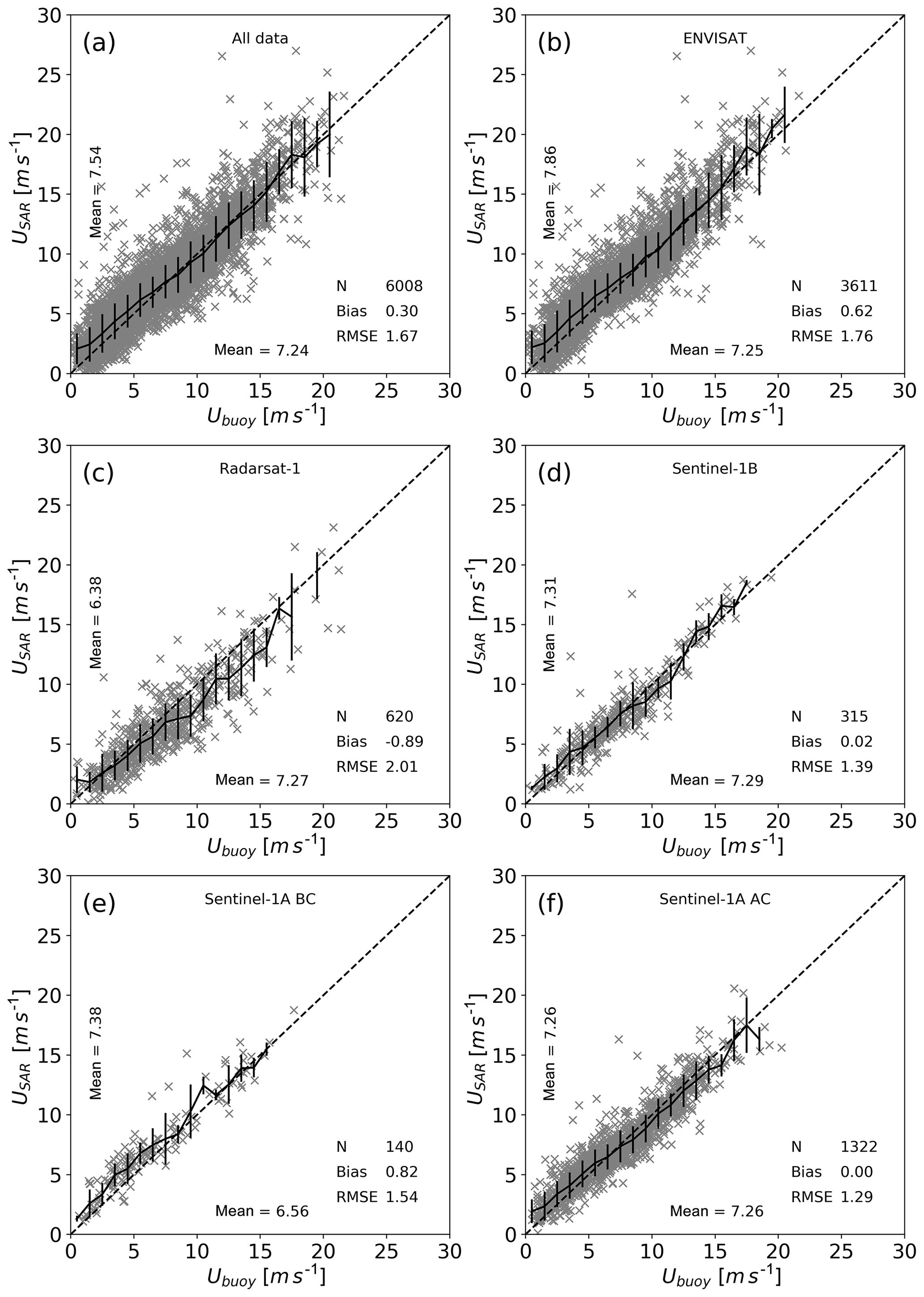
Figure 2 Scatter plots of SAR versus buoy winds at 10 m with default SAR wind processing for (a) all data, (b) Envisat, (c) RADARSAT-1, (d) Sentinel-1 BC, (e) Sentinel-1 AC, and (f) Sentinel-1B. The black curves indicate the mean within each 1 m s⁻¹ bin, and the vertical lines around the mean value indicate 1 standard deviation within this bin.

Figure 3 shows comparisons between SAR and buoy wind speeds after applying the intercalibration process described in Sect. 3.2. Results for all satellites improved the bias from 0.30 to −0.04 m s⁻¹ and the RMSE from 1.67 to 1.46 m s⁻¹. Considering each of the sensors separately, biases lie between −0.2 and 0.03 m s⁻¹, which is a drastic improvement compared to biases in Fig. 2 ranging between −0.89 and 0.82 m s⁻¹. Large improvements are found for Envisat, RADARSAT-1, and Sentinel-1A BC in terms of both biases and RMSE. The two largest datasets, Envisat (Fig. 3b) and Sentinel-1A AC (Fig. 3e), show a higher mean wind speed from SAR when the buoy wind speed is less than 7 m s⁻¹ and vice versa lower mean wind speeds from SAR when buoy wind speeds exceed 9 m s⁻¹. For Envisat, these opposing biases are averaged to nearly zero in the overall bias. Altogether, the intercalibrated SAR winds have smaller biases than the individual datasets and small differences between the sensors compared to the default processing. The following analysis will therefore be based on the intercalibrated SAR wind maps.

Figure 3 Scatter plots of intercalibrated SAR versus buoy winds at 10 m for (a) all data, (b) Envisat, (c) RADARSAT-1, (d) Sentinel-1A BC, (e) Sentinel-1A AC, and (f) Sentinel-1B. The black curves indicate the mean within each 1 m s⁻¹ bin, and the vertical lines around the mean value indicate 1 standard deviation within this bin.

3.3 SAR wind atlas methods

A wind atlas is a map of statistical representations of the wind speed over a designated area. The wind climate is typically represented by a Weibull distribution of wind observations that is characterized by the Weibull scale parameter (A, m s⁻¹) and a shape parameter (k, unitless). They are related to the mean energy density (E, W m⁻²) by

$$\begin{array}{}\text{(1)}& E={\displaystyle \frac{\mathrm{1}}{\mathrm{2}}}\mathit{\rho }{A}^{\mathrm{3}}\mathrm{\Gamma }\left(\mathrm{1}+{\displaystyle \frac{\mathrm{3}}{k}}\right),\end{array}$$

where ρ is the air density and Γ the gamma function. A typical approach in wind energy is to use the Wind Atlas Analysis and Application (WAsP) programme that implements methods from the first European Wind Atlas (Troen and Petersen, 1989). Wind atlases are normally generated from long time series, but it is also possible to use the quasi-instantaneous wind fields derived from SAR (Christiansen et al., 2006). A special version of WAsP developed for satellite-based inputs (S-WAsP) is used here. The Weibull fitting uses second moments as recommended in Pryor et al. (2003). SAR wind images are projected on a regular WGS84 grid with 0.02^∘ cell spacing before processing the data to a wind atlas. The mean wind speed can be defined as the arithmetic mean of the available samples.

$$\begin{array}{}\text{(2)}& U={\displaystyle \frac{\mathrm{1}}{F}}\sum _n{u}_n,\end{array}$$

with the wind speed of the individual image u_n averaged on the 0.02^∘ grid and the total number of observations F.

Results from a SAR-based wind atlas can be noisy because of the high resolution of wind fields and the relatively few samples. Therefore, we apply a Gaussian filter using a standard deviation of 0.03^∘ with a cut-off at 0.06^∘ to smooth the mean wind fields.

Properties of the satellite data acquisition such as temporally fixed overpasses, relatively low sampling, and data truncation lead to uncertainty in a SAR-based wind atlas (Barthelmie and Pryor, 2003). Advanced methods for classifying SAR wind maps are available (Badger et al., 2010), but we choose to apply random sampling considering all images available, which is recommended where more than 400 images are available (Pryor et al., 2003). This approach is also used in earlier SAR-based wind atlases (Hasager et al., 2011). The influence of diurnal cycles is investigated in more detail in Sect. 4.1.1.

SAR images may be acquired for other purposes than wind resource assessment, e.g. sea ice monitoring, and this can influence the temporal coverage of acquisitions. Sea ice detection will mainly occur during the winter months (Sandven et al., 1999). The study domain is located in the mid-latitudes and winds are expected to change with the seasons. We therefore check for seasonal biases in the data acquisition (see also Sect. 4.1.2). For the arithmetic mean wind speed in Eq. (2), the seasonal bias can be corrected by calculating mean wind speeds U_m by month (Monaldo, 2011):

$$\begin{array}{}\text{(3)}& U_{\mathrm{m}}={\displaystyle \frac{\mathrm{1}}{F_{\mathrm{m}}}}\sum _n{u}_{n,\mathrm{m}},\end{array}$$

with the number of observations F_m for each month m and u_n,m the SAR wind speeds occurring in this month. Monthly mean wind speeds are then averaged to a seasonally corrected mean wind speed U_sc:

$$\begin{array}{}\text{(4)}& U_{\mathrm{sc}}=\sum _m{\displaystyle \frac{F_{\mathrm{m}}}{F}}{U}_{\mathrm{m}}.\end{array}$$

S-WAsP is not able to account for seasonal biases in the Weibull parameter estimation. Therefore, no seasonally corrected Weibull parameters or energy densities are available.

4 Results

4.1 Wind resource statistics

In the following, we present the first wind atlas for the US East Coast based on intercalibrated SAR wind fields from four different sensors. Figure 4 shows wind statistics at 10 m: the arithmetic mean wind speed from Eq. (2) calculated from SAR (Fig. 4a) and the mean wind speed from modelled data (WTK) (Fig. 4b). A visual comparison shows similar features. WTK wind speed contours are smoother than those from SAR for two reasons: (i) SAR wind speeds are based on high-resolution observations that can resolve sub-kilometre-scale variation in the wind fields, and (ii) SAR-derived mean winds are derived from fewer samples while WTK winds are based on 7 full years of hourly modelled wind speeds. Wind speeds are lower close to the coast and increase with the distance from shore for both SAR and WTK. A band of high winds is located off the coast of North Carolina and extends to the northwest with higher mean wind speeds in SAR than in the WTK. Horizontal variations in the SAR wind speed are higher than for WTK. The mean wind speeds are lower for SAR than WTK in a region close to the shores of Virginia and Delaware. Another clear difference is the wind speed in the Gulf of Maine. WTK data show mean wind speeds less than 7.5 m s⁻¹ while SAR winds go up to 8.5 m s⁻¹. In both datasets, a feature of lower mean wind speed is present to the southeast of Nantucket but more pronounced in the SAR-derived map.

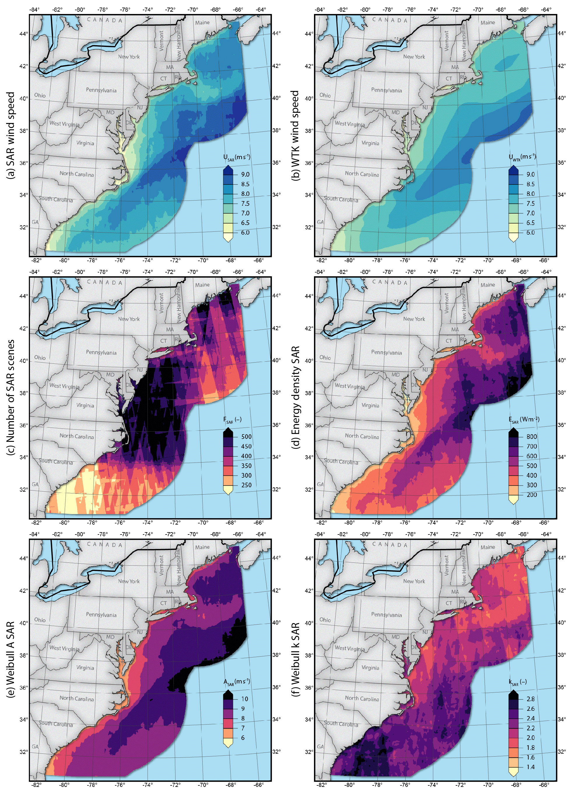
Figure 4 Wind atlas at 10 m a.s.l. (above sea level): (a) arithmetic mean wind speed from SAR, (b) mean wind speed from WTK, (c) number of SAR samples, (d) SAR energy density, (e) SAR Weibull scale parameter A, (f) SAR Weibull shape parameter.

North of 34^∘ latitude, more than 350 samples are used, but fewer than 250 are used off the coast of Georgia (Fig. 4c). The energy density ranges from 200 W m⁻² close to shore to 800 W m⁻² far offshore (Fig. 4d). The Weibull shape parameter A (Fig. 4e) shows similar features as the wind speeds and the energy density. The scale parameter, k (Fig. 4e), ranges between 2 and 3 in the south and 1.75 and 2.5 in the north of the domain. High k values are associated with a narrow Weibull wind speed distribution.

Wind resources and wind roses are compared between SAR, WTK, and in situ buoy measurements for three example locations along the coast in Fig. 5. Buoy 44029 is located in the Gulf of Maine, buoy 44009 is located off the Delaware coast, and buoy 41038 is located off North Carolina; see Fig. 1 for detailed positions. Buoy data are filtered to cover full years (at least 80 % available data) to avoid seasonal sampling biases. Between 7 and 10 years of measurements are available at the buoy locations. WTK covers 7 full years, and the SAR winds are sampled over the entire period from 1998 to 2018 but less frequently. SAR wind speeds are expressed as equivalent neutral winds while the 10 m wind speeds from WTK are stability-dependent wind speeds. Buoy wind speeds are extrapolated accordingly but stability effects are small (less than 0.2 m s⁻¹ differences for the mean wind speed).

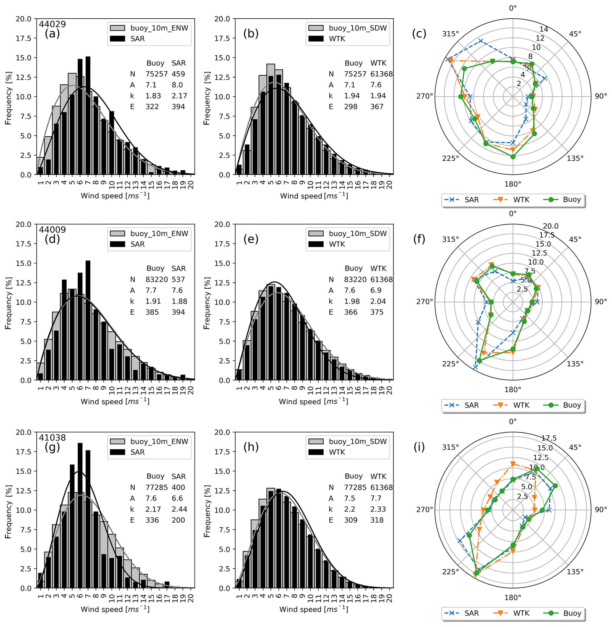
Figure 5 Weibull fits and wind roses for buoys 44029 (a–c), 44009 (d–f), and 41038 (g–i). SAR on the left (a, d, g), WTK in the middle (b, e, h), and wind roses for buoy, SAR, and WTK on the right (c, f, i). Key characteristics are given in the tables: number of observations (N), Weibull shape (A) in metres per second, Weibull scale (k), and the energy density (E) in watts per square metre.

SAR-based results show good agreement at buoy 44009, but distributions are skewed towards higher wind speeds at 44029 and lower at 41038, while WTK distributions generally agree well with the buoy data. Wind directions for SAR show more winds from the northwest for buoy 44029 and agree well with buoy data otherwise. Wind directions from the WTK show most deviations for buoy 41038. There are large deviations ranging from −136 to 72 W m⁻² between wind resources as measured from buoys and SAR that merit closer investigation in the following.

4.1.1 Diurnal cycle

As noted in Sect. 3.3, SAR sensors acquire data at fixed times of the day. We investigate influences of this on the wind retrieval by investigating the diurnal cycle at five buoys located across the study domain. In addition to the three buoys in Fig. 5, we consider a New York buoy (44065) and a Chesapeake Bay buoy (44072). All buoys are within 20 km of the shoreline with the exception of buoy 44009, which is located approximately 60 km offshore. The diurnal variation in the mean wind speed is similar between these buoys with minima between 10:00 and 12:00 LT (local time); see Fig. 6. Buoy 44009 shows less diurnal variation, which might be due to the buoy location further offshore. Overlaid in Fig. 6 is a histogram of the satellite acquisition times showing that images are not randomly sampled due to the polar orbits of satellites. We note that the morning times of ENV overpasses coincide with the minima in the mean wind speeds, while S1A, S1B, and RS1 overpasses are outside this time interval.

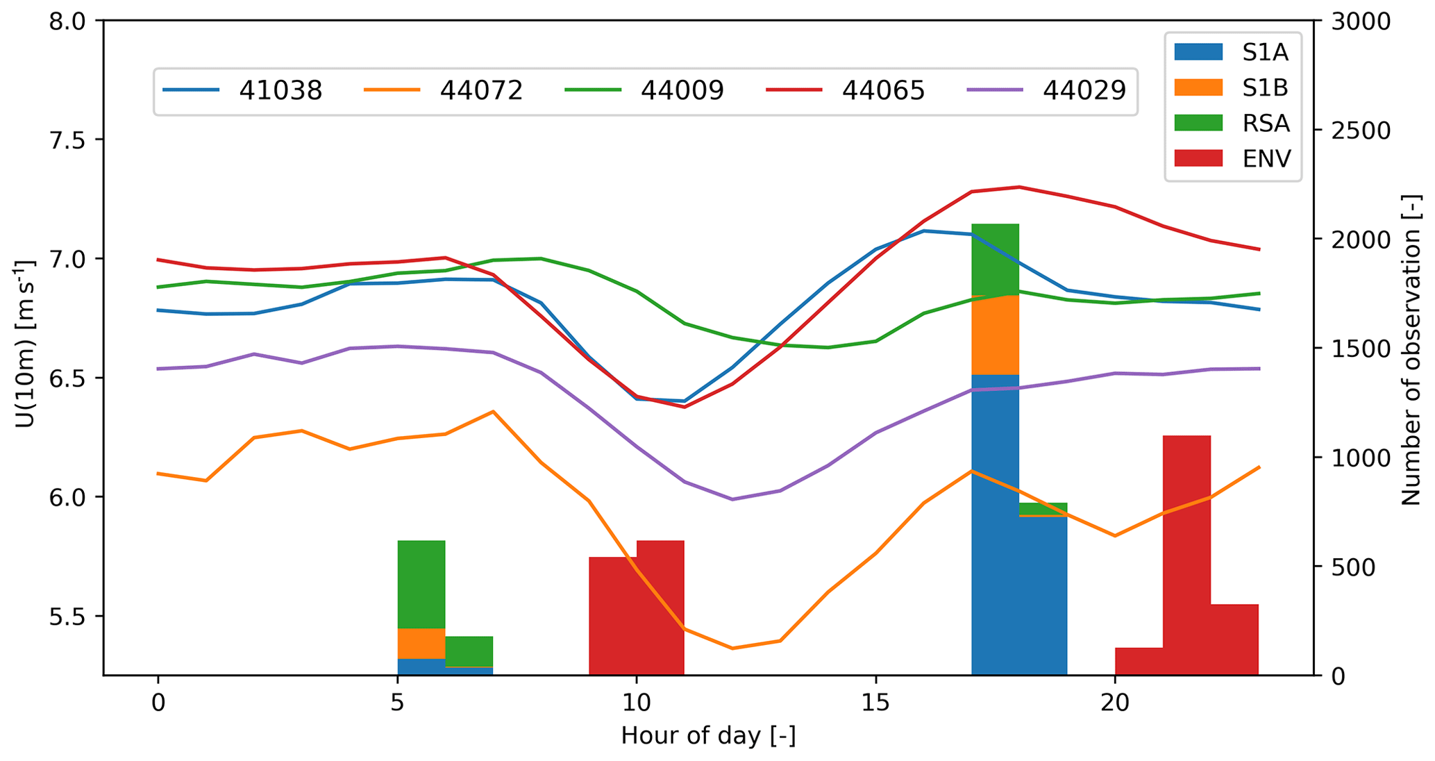
Figure 6 Mean wind speed of selected buoys in local time (UTC−5). The bars indicate the number of satellite observations for RADARSAT (RSA), Envisat (ENV), Sentinel-1A (S1A), and Sentinel-1B (S1B).

4.1.2 Seasonal sampling bias

We investigate seasonal sampling biases in SAR for four regions of 2^∘ by 2^∘ along the US East Coast. Figure 7 shows the spatial average of monthly acquisition frequency F_m∕F and monthly mean wind speed U_m from Eqs. (3) and (4) at four areas. Acquisitions are unevenly distributed over the year. More data are available during the winter in the Gulf of Maine while Delaware and North Carolina are biased towards late summer to early autumn. U_m shows considerable seasonal changes with generally lower winds in summer and higher winds in winter.

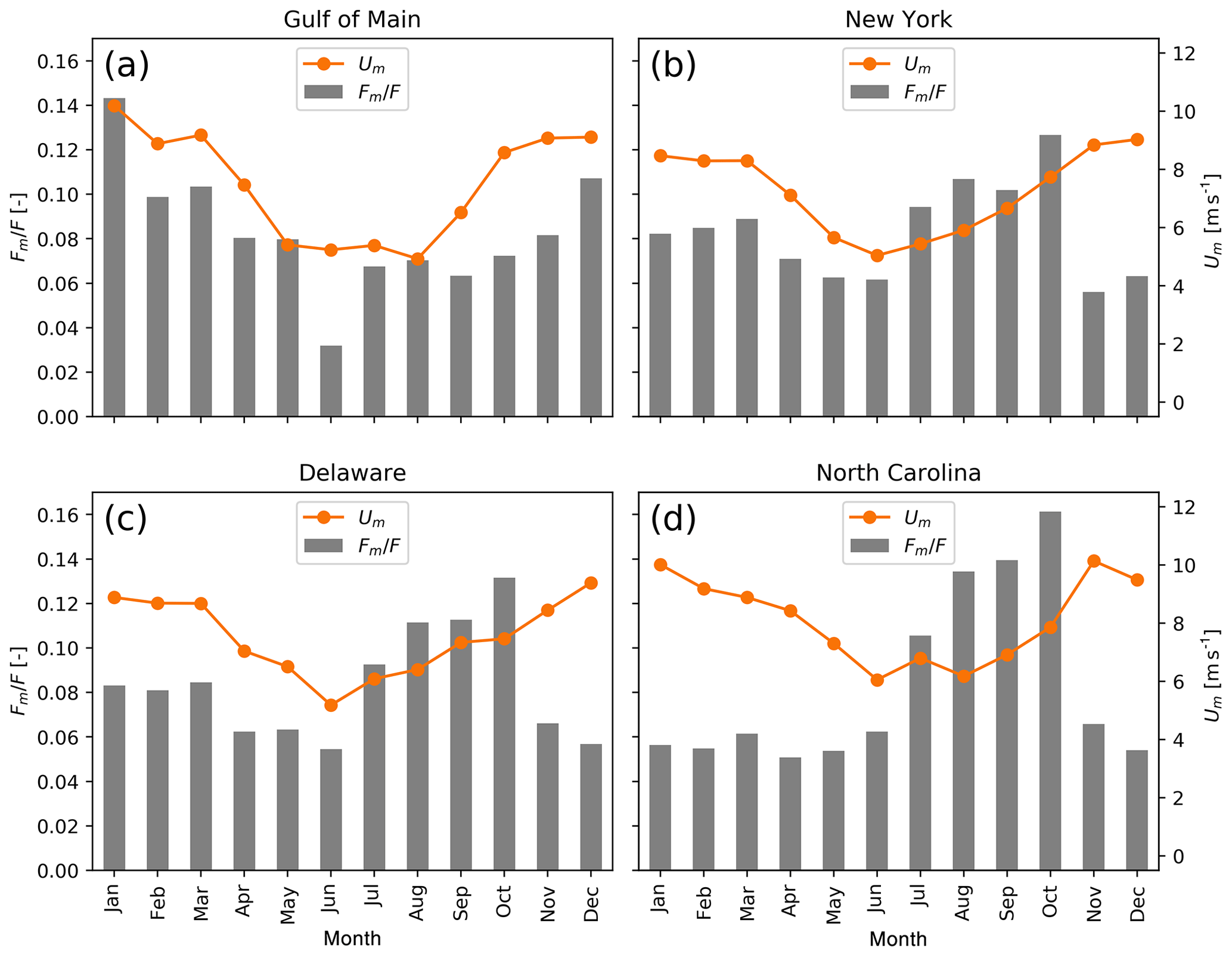
Figure 7 Frequency of data acquisition (F_m∕F) and mean SAR wind speeds (U_m) averaged by month over four regions close to (a) Gulf of Maine, (b) New York, (c) Delaware, and (d) North Carolina.

Figure 7 shows considerable seasonal sampling biases. A seasonally corrected SAR (SAR_SC) mean wind speed map is calculated from Eq. (4) and shown in Fig. 8a together with the differences with respect to uncorrected maps from Fig. 8b. The seasonal correction reduces wind speeds in the north, while it increases wind speeds in the south of the study domain.

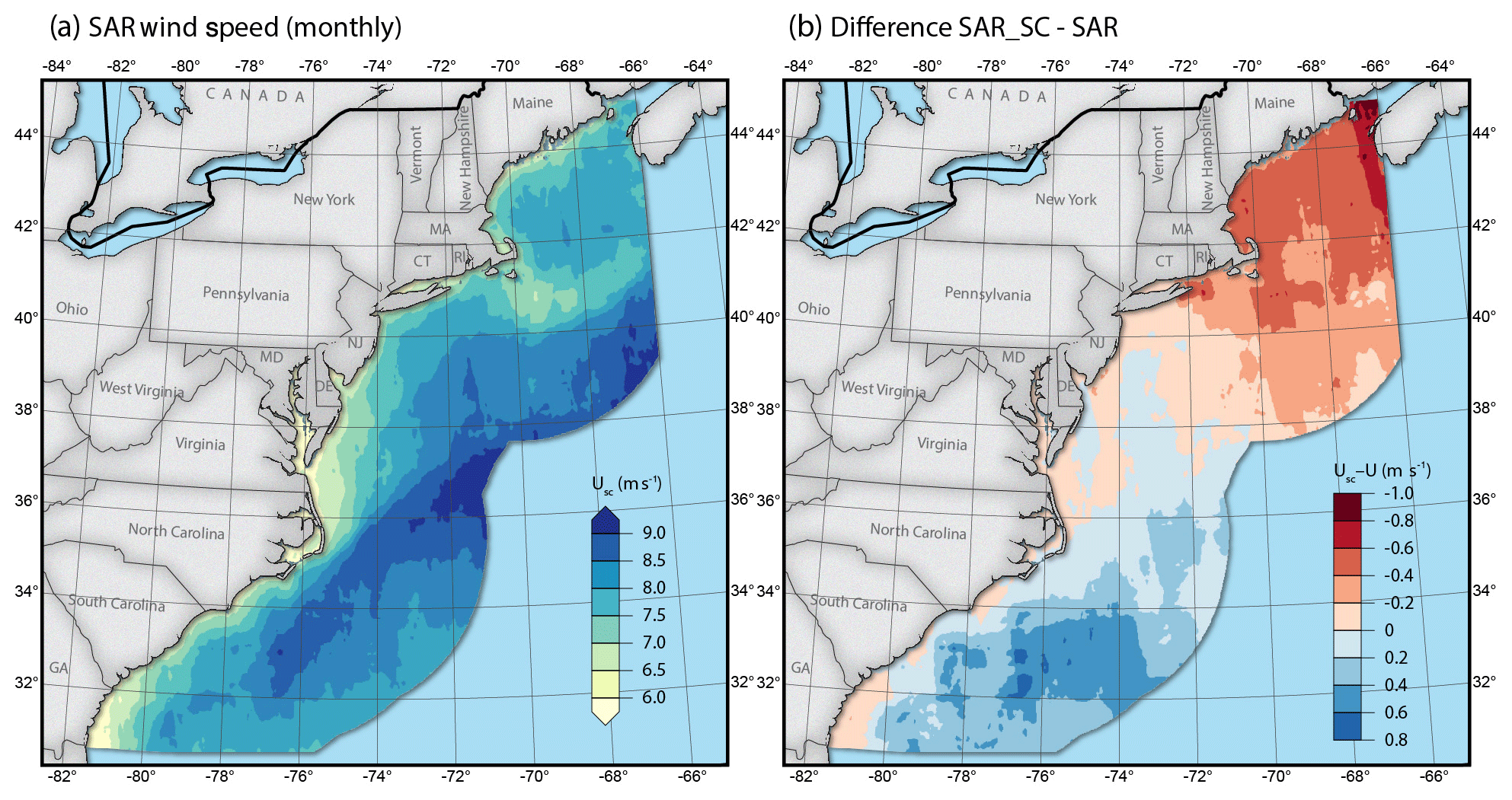
Figure 8 (a) Seasonally corrected SAR wind speed; (b) difference between seasonally corrected and original SAR map.

Two SAR-based mean wind speed maps in Figs. 4a and 8a have been calculated. The one better representing the long-term wind conditions is determined from comparison to long-term mean wind speeds from the ocean buoys. Buoys are required to have at least 7 full years (more than 80 % recovery rate) of measurements. It is necessary to use a representative position for the buoys because buoy positions can change over time and SAR or WTK is not collocated in time. This requires that buoy positions do not change significantly during the measurement period. Buoys 41002 and 44018 are removed because their location changes by more than 100 km. Sixteen buoys fulfil these criteria and statistics on comparisons to the SAR mean wind speed in Fig. 4a, WTK mean wind speed in Fig. 4b, and the seasonally corrected SAR mean wind speed in Fig. 8 are presented in Table 2.

Table 2 Mean absolute error (MAE), root-mean-square error (RMSE), and bias between mean wind speeds from buoys versus SAR, seasonally corrected SAR (SAR_SC), and WTK.

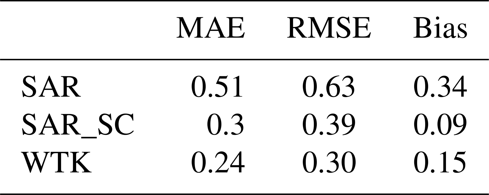
The seasonally corrected mean wind speed from SAR (SAR_SC) shows a lower RMSE, MAE, and bias than the uncorrected SAR dataset. We consider SAR_SC a better representation of the seasonality, and it will therefore be used for comparisons with the WTK in Sect. 4.2.

4.2 Spatial wind variability from SAR and WTK

To compare SAR_SC and WTK mean wind speeds in the coastal zone, we define transects perpendicular to the generalized coastline of the United States up to 100 km from the shoreline. Because of the complexity of the shoreline, a compromise needs to be found between perpendicular transects, avoiding crossing transects, and the definition of distance to shore for convex corners. The resulting transects are shown in Fig. 9 and are labelled with unique identifiers (transect_id) ranging from 0 in the north to 650 in the south.

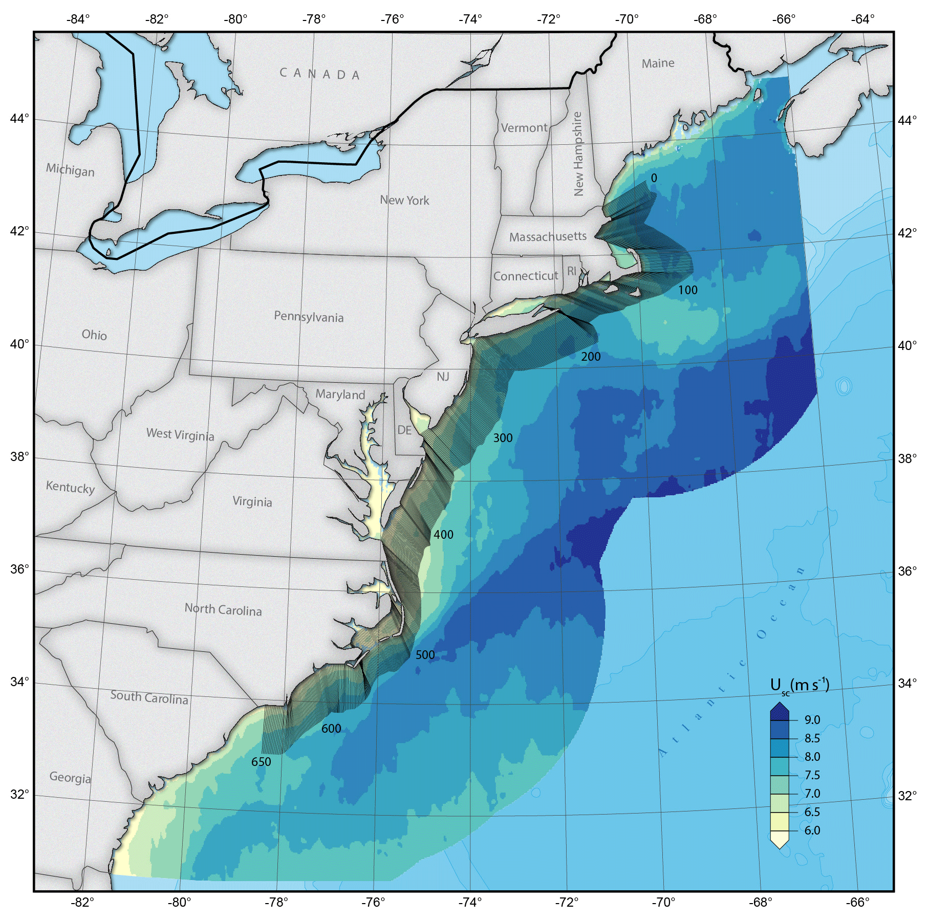
Figure 9 Seasonally corrected SAR mean wind speed maps (SAR_SC) with transects perpendicular to shore (every fifth transect is plotted). Starting at transect_id 0 in the Gulf of Maine going to transect_id 650 off North Carolina.

Wind speeds are linearly interpolated along each transect every 2 km. Figure 10 shows the wind speeds per transect ID and as a function of distance to shore. These plots can be seen as a horizontal sheet of mean wind speeds along the coastline perpendicular and parallel to shore. The white areas are land contamination in SAR wind maps originating from islands not accounted for in the generalized coastline. Again, we can see similarities in the features on large scales with a band of high wind speed between transect_id 500 and 600 but also smaller features like an increased wind speed at the mouth of the Delaware River around transect_id 350.

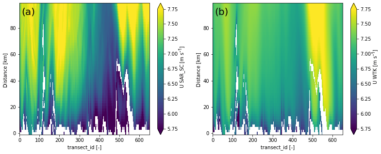
Figure 10 Mean wind speeds at 10 m a.s.l. (above sea level) for all transects as a function of the distance to shore. (a) SAR_SC; (b) WTK.

The presentation of wind speeds in Fig. 10 represents spatial structures of the mean winds along the coast but it is hard to assess differences visually. We will focus on wind speed variations in two directions: along-shore and perpendicular to the coastline. The latter is commonly referred to as a coastal wind speed gradient.

4.2.1 Along-shore variation

Figure 11 shows wind speed transects along the shore averaged over distances to shore of [10, 20], [20, 30], [40, 60], and [60, 100] km. From transect_id 0 to 300 the two transects closest to shore (Fig. 11a and b) show remarkably good agreement, both absolute and in shape. Further offshore, in Fig. 11c and d, the positions of local maxima and minima are similar but the amplitude of these features is larger for SAR_SC than WTK. From transect_id 300 onward (southward), SAR_SC gives consistently lower wind speeds with the exception in Fig. 11d around transect_id 570 and 650.

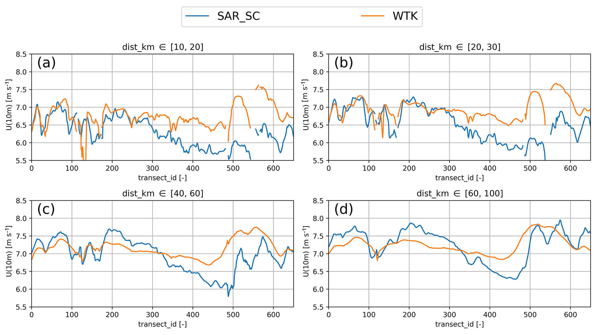
Figure 11 Along-shore variation in the mean wind speeds for distance to shore intervals of (a) [10, 20], (b) [20, 30], (c) [40, 60], and (d) [60, 100] km.

The region closer than 60 km to shore is most relevant for wind farm development. Here, SAR observations suggest high wind speeds in the north up to transect_id 250, while WTK consistently shows higher wind from transect_id 500 southward.

4.2.2 Coastal gradients

Wind speeds averaged over the distance to shore for six regions are shown in Fig. 12. All regions show coastal gradients with the typical increase in mean wind speed with distance from the shoreline. For Fig. 12a, around Nantucket, there is very good agreement both in the gradient and in the absolute value. Figure 12b, c, and f show similar behaviours, with SAR_SC exhibiting lower wind speeds closer to shore but higher gradients resulting in higher wind speeds further offshore. Gradients are similar for Fig. 12d, but SAR_SC winds are offset by 0.7 m s⁻¹ toward lower wind speeds. The most pronounced differences in terms of wind speed gradients are found around Pamlico Sound (Fig. 12e) with SAR_SC winds up to 1.5 m s⁻¹ lower close to shore and a steep gradient from 40 to 100 km offshore.

Figure 12 Mean wind speeds averaged over several transects covering six different regions. The panels are as follows from north to south: (a) Nantucket, (b) Long Island, (c) state of New York, (d) Virginia to Delaware, (e) Pamlico Sound, (f) southern part of North Carolina.

The transects show consistently higher wind speed gradients with the exception of the most northern region around Nantucket (Fig. 12a). The wind speed gradient is defined as

$$\mathrm{grad}={\displaystyle \frac{\mathrm{d}U}{\mathrm{d}x}},$$

where U is the mean wind speed and x is the distance to shore. The wind speed gradient is averaged for each transect resulting in 650 mean gradients for SAR_SC and WTK and the distribution is shown in Fig. 13. Mean gradients are mostly positive, indicating higher wind speeds further offshore as expected. For WTK, the distribution is almost symmetric with a mean of 0.91 m s⁻¹ per 100 km. The distribution from SAR_SC is more skewed and clearly separated from the WTK. The mean of the distribution is 1.40 m s⁻¹ per 100 km, which is considerably higher than for the WTK.

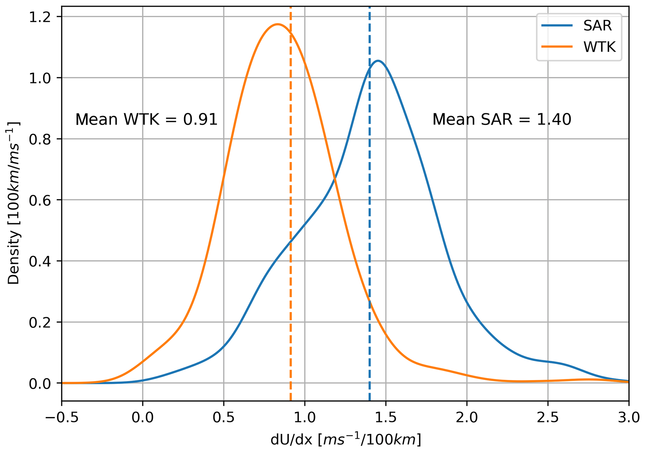
Figure 13 Density plot of wind speed gradients from SAR and WTK. Dashed lines indicate the mean values.

4.2.3 Wind resource variation within bureau of offshore energy management areas

Wind farm development is allowed within the limits of the offshore lease areas defined by the BOEM; see Fig. 14. Because lease areas are typically several hundred square kilometres large, wind resources are expected to vary within each of the areas. Information on the magnitude of this variation is needed for wind farm development.

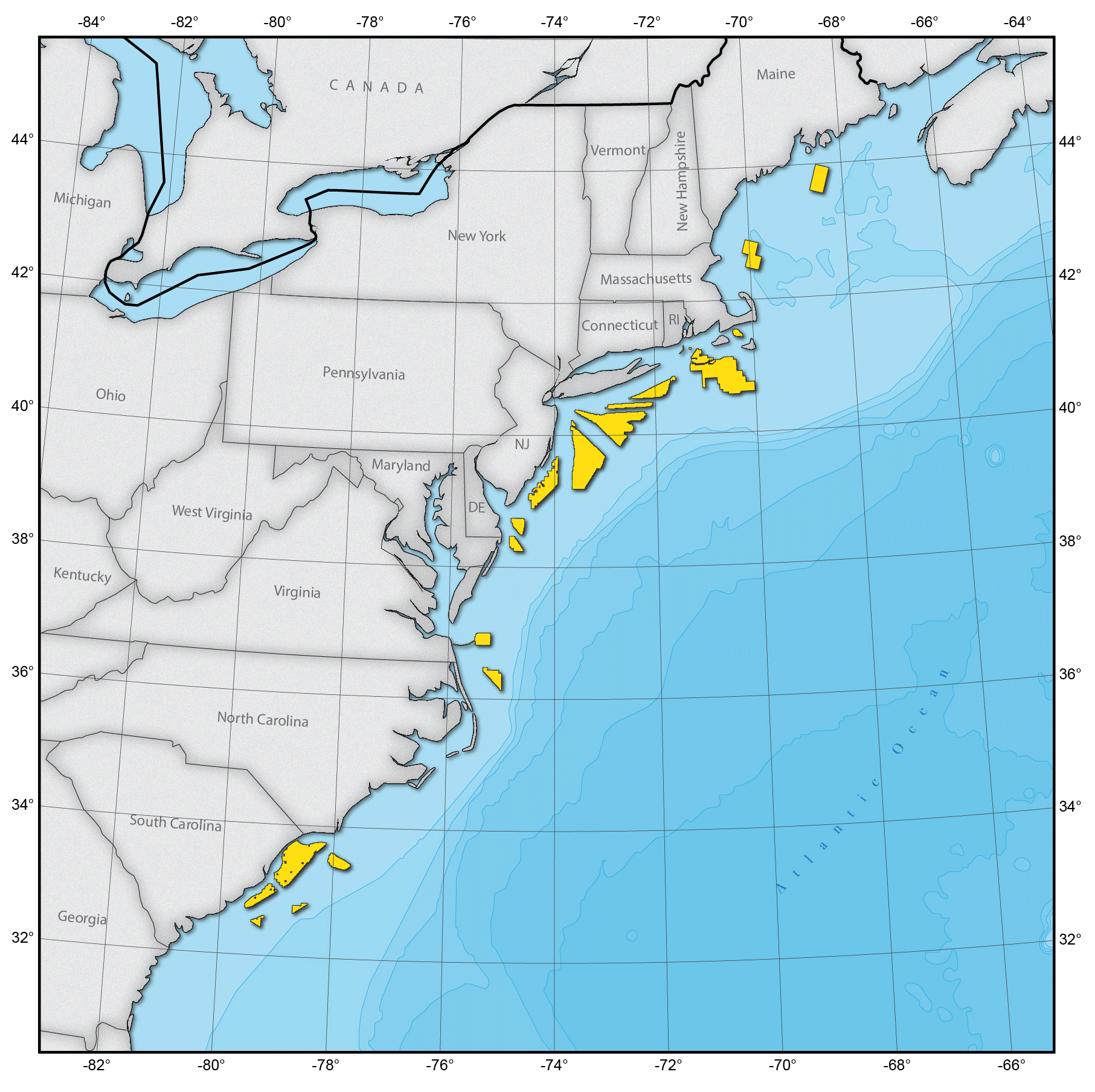
Figure 14 Bureau of Offshore Energy Management lease areas for the US East Coast. Colour codes are used to differentiate different areas.

We select mean wind speeds from SAR_SC and the WTK at all grid points within a given lease area. The distribution of mean wind speeds within each area is then calculated and presented as a violin plot in Fig. 15. The variation in mean wind speeds is higher from SAR for all areas except Cape Wind and Kitty Hawk. The average of the differences between minimum and maximum is 0.2 m s⁻¹ for the WTK and 0.47 m s⁻¹ from SAR_SC. This indicates that the WTK predicts much less variation in wind resources within a potential wind farm site than SAR_SC. Note that a mesoscale numerical weather prediction model, such as the model behind WTK, is unable to pick up wind speed variations on the order of 0.5 m s⁻¹, and their RMSEs are typically more than 0.5 m s⁻¹.

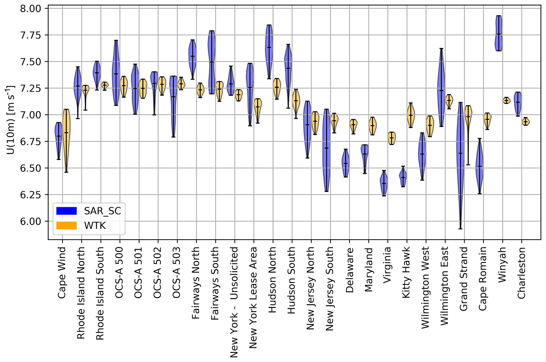
Figure 15 Violin plot for wind speeds from seasonally corrected SAR and WTK. Potential lease sites are ordered from north (left) to south (right).

5 Discussion

In the following, we discuss the results from the evaluation of the SAR wind atlas and the associated artefacts from the sampling. The representation of wind speed variations in the coastal zone is discussed as retrieved from SAR and modelled in the WTK.

5.1 Validation of intercalibrated SAR wind archive with buoys

This study presents the first SAR wind atlas merging archives from four sensors into a consistent dataset. Extensive comparisons with buoys show that even though data are processed consistently with CMOD5.N, biases between the sensors range from −0.89 to 0.62 m s⁻¹ (see Fig. 1), which is similar to results from northern Europe. Badger et al. (2019) suggested intercalibration to remove biases by adjusting the NRCS as a linear function of the incidence angle using modelled wind speed and direction inputs. Those adjustments decrease the difference in biases between sensors to 0.2 m s⁻¹. Overall, a tendency to overestimation for low wind speeds and underestimation for high wind speeds remains in the SAR wind maps, which influences the Weibull fitting performed here. Two findings speak for the generality of this approach: (i) intercalibration tables derived over northern Europe can be applied for the US East Coast; (ii) applying the suggested intercalibration method to RADARSAT-1 data reduces the bias to 0.03 m s⁻¹. The intercalibration should in no way substitute efforts to better understand scattering mechanisms in order to improve the calibration of NRCS as well as GMFs for wind retrieval (Troitskaya et al., 2018). Tuning NRCS values is an application-driven approach, which is necessary at present in order to produce wind maps with consistently low biases. This approach is significantly different from previous and current efforts to determine the most suitable GMF for SAR wind retrievals (Christiansen et al., 2006; Takeyama et al., 2013).

5.2 SAR wind atlas for the US East Coast

We have produced a SAR-based wind atlas of the US East Coast covering the coast from Georgia to the Canadian border. An alternative to SAR measurements are scatterometers (Stoffelen and Anderson, 1997). From a wind resource perspective, their main advantage is the higher temporal resolution, but it comes at the cost of a lower spatial resolution of typically 25 km. Merging SAR and scatterometer wind data to create a wind atlas has been done (Doubrawa et al., 2015; Hasager et al., 2015), but this approach needs further refinement to fully utilize the high temporal coverage from scatterometers and the high spatial resolution from SAR.

We have estimated the Weibull parameters A and k, energy densities, and mean wind speeds from all the available SAR wind maps; see Fig. 4. The energy density, Weibull shape (A), and mean wind speed generally increase with the distance from shore. The Weibull scale parameter (k) is high in the south and lower in the north. The Weibull k parameter requires more samples than wind speed or shape parameter to be correctly estimated (Barthelmie and Pryor, 2003). The area with high shape parameters coincides with a low number of samples and significant seasonal biases in the sampling, which casts doubt on the accuracy of results in these instances.

For the purpose of comparing the SAR-based wind atlas to the WTK, it is desirable to keep the SAR data as independent from modelling results as possible. Therefore, we have not utilized any information from the WTK dataset to perform stability correction of the SAR winds. The buoy observations used in this analysis indicate that for heights of 10 m or less above the sea surface, atmospheric stability effects on the wind speed are smaller than 0.2 m s⁻¹ on average. It is however possible that larger deviations from the neutral wind profile occur for specific instances.

The presented SAR wind atlas is calculated at a 10 m height above the sea surface. However, for wind energy applications, estimates closer to turbine hub heights at 100 m or higher above sea level would be more desirable. Extrapolation of the wind atlas results presented here is possible using model-derived stability corrections to the long-term average wind profile (Badger et al., 2016). The extrapolation would first require a careful validation of the model outputs against buoy observations and is therefore beyond the scope of this study. The vertical extrapolation would increase the applicability of the SAR-derived wind speeds for wind energy purposes and will be considered in the future. Our wind atlas and comparisons at the 10 m level represent a valuable first step, which helps us assess differences between datasets and gain insight into the horizontal variation in wind resources.

5.3 Wind resource comparisons

This study shows a comparison between SAR and WTK, assuming that both are representative for the wind climatology. A method to sample SAR winds according to wind classes based on modelled climatology is available to reduce the number of samples necessary for wind resource assessment (Badger et al., 2010). This has the advantage of choosing SAR images that are more representative for the large-scale wind conditions but comes with the disadvantage of weakening the independence of the SAR-derived results. Combining data with other in situ observations as done in Doubrawa et al. (2015) is an option, but the density of measurements on the US East Coast is lower than in the Great Lakes, where the method was developed.

SAR-derived wind resources overestimate the energy density by 72 W m⁻² at buoy 44029 and underestimate them by 136 W m⁻² for buoy 41038. Sampling of the SAR images shows considerably uneven sampling between different seasons (Fig. 7). In the region of buoy 44029, the winter months with high wind speeds are overrepresented. Wind resource estimates derived from these data will retain a bias to higher wind speeds and thus overestimate the wind resource, which is in line with our observations. For buoy 41038, an opposing bias towards summer and early autumn associated with low wind speeds could explain the underestimation of wind resources. The resource estimate from SAR shows little difference in Weibull parameters and the energy density for buoy 44009. In this region, seasonal sampling is more evenly distributed and oversampling occurs between the extrema. Wind resource estimates from the WTK have been made at the same buoy locations. Generally, the wind resources are estimated more accurately than from SAR, but overestimations of 69 W m⁻² occur at buoy 44029.

SAR wind atlases for other regions have generally not reported seasonal dependency in the data coverage (Hasager et al., 2011; Karagali et al., 2014). We have implemented a simple method to overcome this problem using weighted monthly averages to calculate the mean wind speed (Eq. 4) (Monaldo, 2011). This seasonally corrected mean reduces wind speeds in the north, while increasing them in the south of the study domain. Differences frequently exceed 0.5 m s⁻¹, which are substantial for a product that should be used in the context of wind energy. The seasonally corrected mean wind agrees better with long-term means from buoy observations (Table 2), in terms of both mean errors and RMSE, and we consider them a better choice when estimating a wind climatology. Using monthly weights in the estimation of SAR-derived Weibull parameters should be possible, but implementing and validating such a method is beyond the scope of this article.

5.4 Influences of diurnal variability

SAR satellites operate on orbits with fixed times for ascending and descending tracks 12 h apart. This sampling pattern influences results in our wind atlas. The time of day of the observations from Envisat is approximately 10:00 and 22:00 LT, while Sentinel-1A/B and RADARSAT-1 observe around 05:00 and 17:00 LT. Envisat contributes the most observations in this study, and thus its temporal bias will largely influence results. For buoy 44072 located in the Chesapeake Bay, both Envisat acquisition times are close to a local minimum of the wind speed. Therefore, a bias towards underestimating the climatological mean wind speed is expected here. For SAR mean winds at the remaining buoy locations displayed in Fig. 6, the effect from diurnal variability will be smaller but still present. Adding more Sentinel-1 acquisitions will even out the diurnal sampling bias from Envisat.

Sea breeze phenomena present in this region contribute to diurnal wind speed variations (Hughes and Veron, 2015). The influence of the diurnal cycle is more pronounced closer to shore. SAR images that happen to oversample the wind speed minimum of the diurnal cycle would cause a stronger bias towards lower wind speeds closer to shore than farther offshore. Wind observations sampled in such a way would artificially increase the coastal gradient.

5.5 Wind speed gradients from SAR and WTK

Mean wind speed maps from SAR and WTK have been compared in this study. Mesoscale models are known to have higher uncertainties offshore if winds come from land (Hahmann et al., 2015). For the buoy locations in Fig. 5, westerly winds come across land, and the wind roses show that these directions occur frequently. For these directions, coastal wind speed gradients occur, caused by the roughness change between land and sea. Coastal gradients from SAR have been shown to agree well with lidar wind speeds for the first few kilometres from shore (Ahsbahs et al., 2017). The SAR-based wind atlas has a resolution of 0.02^∘ that makes it ideal for investigating horizontal variations in the mean wind speed and serving as a reference for modelled wind speed gradients from the WTK.

Wind speeds from SAR are typically lower than those from the WTK close to shore but gradients from SAR are higher than from the WTK for most regions (Fig. 12b, c, e, and f). At 100 km from the shoreline, SAR tends to give higher winds than WTK. Wind speed gradients show that SAR winds, on average, show an increase of 1.40 m s⁻¹ per 100 km. For the WTK, this value is only 0.91 m s⁻¹ per 100 km. Fixed times of the satellite tracks could influence wind speed gradients if they show diurnal variability. This cannot easily be investigated from buoy measurements because they lack the spatial coverage, which was the initial motivation for this study. The influence of sampling biases is unlikely the sole source for the observed differences in the wind speed gradients.

A long-standing challenge in SAR wind analysis has been that neutral stratification of the surface layer must be assumed. The effect of this assumed neutral stratification of the surface layer is a wind speed bias that depends on the stability of the atmospheric surface layer. The SAR-derived wind speeds are too low in regions where the surface layer is stable, because wind speed must compensate for the too high (i.e. neutral rather than stable) drag coefficient assumed. Likewise, the SAR-derived wind speeds are too high in regions where the surface layer is unstable, because wind speed must compensate for the too low (i.e. neutral rather than unstable) drag coefficient assumed. Basically, the SAR-derived wind has to compensate for the lack of the stability dependence of the vertical mixing of momentum in the surface layer. This is reflected in our study in the observation that SAR winds are faster than buoy winds over the Gulf Stream (where the atmospheric surface layer is destabilized by the warm underlying water) and slower than the buoy winds over the cold waters north of the Gulf Stream (where the atmospheric surface layer is stabilized by the cool underlying water). Results from earlier resource assessments in Dvorak et al. (2013) using WRF show that wind resources generally increase going from south to north in our investigated domain but show less variability than both SAR and WTK.

Spatial variations in the mean wind speed within lease areas for wind farm development were investigated using the SAR and WTK data (Fig. 15). For most areas, WTK shows less variation than SAR. For example, mean wind speeds from the WTK for “New Jersey South” range from 6.8 to 7.0 m s⁻¹. Low variation like this might lead a developer to neglect horizontal wind speed gradients at their site, i.e. during the planning of a measurement campaign. At the same location, SAR wind speeds range from 6.3 to 7.1 m s⁻¹. This variation is substantially larger, suggesting that wind speed variation within this area should be considered. SAR wind maps resolve more variation than mesoscale models or scatterometers, which can explain part of the increased variation (Karagali et al., 2014). Another reason could be speckle noise in the SAR images themselves, but spatial and temporal averaging, as performed in this study, will greatly reduce this effect. Variations found here are in line with previous studies from the Anholt wind farm in Denmark, which is located downstream of a complex coastline and can experience strong wind speed gradients (Ahsbahs et al., 2018; Peña et al., 2018).

5.6 Future work

This study has utilized the COARE 3.0 bulk flux algorithm to account for the effects of atmospheric stability on the vertical extrapolation of buoy winds. This same stability correction could be used to convert the SAR-derived surface stress to stability-aware SAR winds given that the air–sea temperature difference for any point in the area of interest can be obtained from the WTK dataset. The neutral drag law could be used to convert the neutral-equivalent SAR-derived winds to surface stress, and then the equations from the COARE 3.0 bulk flux algorithm could be applied to convert that surface stress back to a stability-aware 10 m wind. This would be a major advance for SAR wind analysis and represents a natural next step for our analysis of wind resources along the US East Coast.

With an increasing archive of Sentinel-1 data, future wind atlases will be based on samples, which are more distributed over the time of day. The rapid growth of our SAR data archives over time will in itself improve the accuracy of wind resource statistics. Further, a weighting of the SAR scenes by month could partly overcome seasonal biases and give better estimations of the Weibull parameters while retaining the observational character of a SAR-based wind atlas.

6 Conclusion

Using a large number of collocated buoy measurements, we have shown that SAR wind fields from different sensors can be intercalibrated. The derived SAR wind atlas is novel in two regards: (1) it ensures consistent calibration towards wind retrievals from different sensors, and (2) it covers the US East Coast where a similar product has not been available before. The presented sensors show seasonal sampling biases that are inconsistent over the study domain, but mean wind speeds can be down to a bias of 0.09 m s⁻¹ and an RMSE of 0.39 m s⁻¹ relative to long-term buoy observations.

Comparisons of the long-term mean wind speeds at 10 m between SAR and WTK indicate that: (1) the model could under-predict the horizontal wind speed gradient with respect to the distance to shore, and (2) wind speed variations within areas designated for offshore wind farm development are lower in the WTK than with SAR. These findings raise awareness that spatial variations in wind resources might be underestimated in this mesoscale model. SAR-derived wind atlases can serve as independent data sources most useful in the early planning phase of an offshore wind farm project.