the Creative Commons Attribution 4.0 License.
the Creative Commons Attribution 4.0 License.
 | 27 Oct 2020
Characterisation of the offshore precipitation environment to help combat leading edge erosion of wind turbine blades
Robbie Herring
Kirsten Dyer
Paul Howkins
Carwyn Ward
Greater blade lengths and higher tip speeds, coupled with a harsh environment, have caused blade leading edge erosion to develop into a significant problem for the offshore wind industry. Current protection systems do not last the lifetime of the turbine and require regular replacement. It is important to understand the characteristics of the offshore environment to model and predict leading edge erosion. The offshore precipitation environment has been characterised using up-to-date measuring techniques. Heavy and violent rain was rare and is unlikely to be the sole driver of leading edge erosion. The dataset was compared to the most widely used droplet size distribution. It was found that this distribution did not fit the offshore data and that any lifetime predictions made using it are likely to be inaccurate. A general offshore droplet size distribution has been presented that can be used to improve lifetime predictions and reduce lost power production and unexpected turbine downtime.
- Article
(1104 KB) - Full-text XML
- BibTeX
- EndNote


The offshore wind industry's need for larger rotors and higher tip speeds has caused blade leading edge erosion to develop into a major problem for the industry. Leading edge erosion is caused by raindrops, hailstones and other particles impacting the leading edge of the blade and removing material. This degrades the aerodynamic performance of the blade and requires operators to perform expensive repairs. The issue has grown in prominence recently with reports that Ørsted had to make repairs to up to 2000 offshore wind turbines after just a few years of operation (Finans, 2018).
The industry attempts to prevent the onset of leading edge erosion by applying protection systems, such as coating and tapes, to the blade leading edge. However, currently these do not last the lifetime of the turbine and require regular replacement.
Several analytical models that aim to estimate the expected lifetime of a protection system have been developed (Eisenberg et al., 2018; Slot et al., 2015; Springer et al., 1974). Finite-element models that can predict the stresses and strains in a protection system from an impinging water droplet have also been produced (Keegan et al., 2012; Doagou-Rad and Mishnaevsky, 2020). To model leading edge erosion, it is important to understand the characteristics of the impinging hydrometeors and, as rain is the most frequent hydrometeor, the droplet size distribution (DSD) of the impinging rain.
The aim of the industry is to develop a methodology that can predict the lifetime of a protection system on a wind turbine from rain erosion tests. The DNV GL project COBRA aims to address this, and Eisenberg et al. (2018) propose using the Springer model. Due to the lack of an offshore dataset, the project uses the onshore Best distribution published in 1950 (Best, 1950). However, the manual measurement techniques used by Best are outdated and have been found to provide inaccurate results (Kathiravelu et al., 2016). The lack of an offshore dataset introduces uncertainty into lifetime predictions, and, as a result, inaccuracies may exist. In this work, state-of-the-art measurement techniques have been used to characterise the offshore precipitation environment and provide the required offshore dataset. A general offshore DSD is presented.
The most widely used DSD is the Best distribution. Best takes the work of several authors and converts them into a common DSD defined as
where F is fraction of liquid water in the air comprising drops with diameters of less than x; I is the rate of precipitation; and
where A=1.30, p=0.232 and n=2.25. Best concluded that the constant n is independent of the precipitation intensity.
This is commonly presented in the literature as
Data were predominantly collected by two manual methods; the “stain” method and the “flour pellet” method. In the stain method, a sheet of absorbent paper is exposed to the rain for a short time. The stains made by the droplets are rendered permanent by previously treating the paper with a suitable powder dye. Then, the stains are counted, measured and interpreted in terms of drop sizes. A calibration curve specific to the filter paper is used to relate the stain diameter to the droplet diameter. The spread factor relationship is dependent upon the physical properties of the fluid, drying conditions and the impact velocity of the droplet (Sommerville and Matta, 1990). In the flour pellet method, rain is allowed to fall into pans of silted flour. The resulting dough pellets are baked and subsequently sized by being passing through graded sieves.
In both measurement techniques, sampling can only occur in short intervals. Best performs measurements using the stain method for a maximum of 2 min. During prolonged periods of sampling, the droplet stains and pellets can overlap, making it difficult to accurately measure and count individual drops. Furthermore, the techniques have a low resolution. Best registers droplet sizes in 0.5 mm intervals. Given that the distribution predicts that for a rain rate of 1 mm h−1, most droplets are between 0 and 2 mm, it is clear that a higher resolution is required for effective analysis.
Two Campbell Scientific PWS100 disdrometers have been installed onto Offshore Renewable Energy Catapult's offshore anemometry hub, which is located 3 nautical miles (5.56 km) from the coast of Blyth, Northumberland. Figure 1 shows the position of the two disdrometers, with the first mounted on the existing platform 25 m a.s.l. (above sea level; disdrometer A) and the second mounted 55 m a.s.l. (disdrometer B). Each disdrometer consists of two photodiode-sensing heads, one near-infrared diode laser head, and one CS215 temperature and humidity sensor. The sensor heads are positioned 20∘ off-axis to the system unit axis, introducing a time lag between the two sensors that enables the fall velocity and size of particles to be calculated.
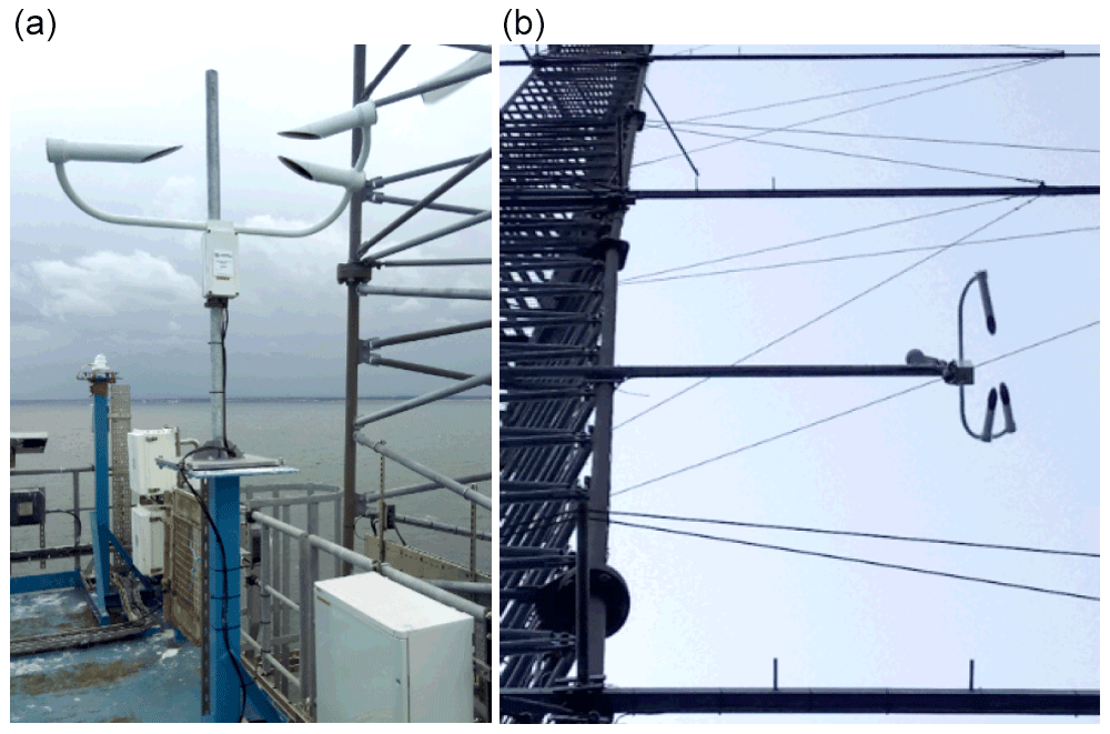
Figure 1The optical disdrometers mounted to the platform (a) and at 55 m a.s.l. (above sea level) (b).
Optical disdrometers are non-intrusive and do not influence drop behaviour during measurement. They have also been shown to successfully resolve droplet break-up and splatter problems experienced by other measurement techniques (Kathiravelu et al., 2016). Agnew (2013) explored the performance of the PWS100 at a site in southern England, finding that the device slightly underestimates the number of droplets with a diameter below 0.8 mm. However, the measurement of larger, more damaging droplets was found to be accurate. Montero-Martínez et al. (2016) compared the performance of the disdrometer during natural rain events in Mexico City to results from a beam occlusion disdrometer and a reference tipping bucket. The PWS100 recorded greater amounts of precipitation than the reference, but the study was unable to back this up statistically and no significant differences in precipitation estimation was found between the disdrometers. Montero-Martínez et al. (2016) concluded that the two devices performed similarly and that the PWS100 provides reliable precipitation measurements. Johannsen et al. (2020) studied the PWS100 against a Thies CLIMA laser precipitation monitor and an OTT Parsivel at a site in Austria. In contrast to Montero-Martínez et al. (2016), the PWS100 recorded less than the reference rain gauge in all but two events. The PWS100 recorded 3 % less total precipitation than the rain gauge across the measurement period, outperforming the Thies and the Parsivel instruments which recorded 20 % and 30 % less, respectively, and the PWS100 was consistently closest to the rain gauge reading throughout the period. Similar drop sizes were recorded between the PWS100 and the Parsivel, with Johannsen et al. (2020) noting that the PWS100 tended to record slightly faster and larger drops. The studies show that there are uncertainties in the accuracy of all disdrometers, with the PWS100 used in this study performing comparatively with or better than the other examined disdrometers.
DSD data from 1 September 2018 up to and including the 31 August 2019 are presented to provide a 12-month period for analysis. This allows analysis to also be completed seasonally. Hydrometeor diameters have been recorded with a resolution of 0.1 mm. Data are available with a time interval of 1 min.
4.1 Quality control
Raw data were received from the disdrometers, and, therefore, detailed quality control was completed before subsequent analysis in line with recommendations from Hasager et al. (2020), Chen et al. (2016) and Vejen et al. (2018). Duplicate records were assessed by comparing timestamps, with any identical timestamps eliminated from the dataset. The meteorological parameters were also evaluated to remove entire duplicate records. It may be possible for a few parameters to be the same; however an entire row of identical parameters is extremely unlikely, and consequently duplication has almost certainly occurred. A gross value check was completed to remove unrealistic and impossible values. Certain parameters are constrained within limits, such as relative humidity, which is given as a percentage, whereas other parameters, such as droplet size, can be evaluated against sensible threshold values. Furthermore, precipitation events where the disdrometer recorded a rain rate of 0 mm h−1 but hydrometeors were recorded were removed, as were events within the bounds of disdrometer error, such as those with a duration of 1 min or where fewer than 10 total hydrometeors were recorded. Particle type classification is determined by the C215 sensor on the disdrometer, which distinguishes particles based on an algorithm using the temperature, wet-bulb temperature and relative humidity. The outputs from the sensor were evaluated against an air temperature threshold, commonly used to distinguish between snow and rain events (Jennings et al., 2018), with any errors being manually inspected.
The consistency between disdrometers was also explored. No sensible results were recorded by disdrometer A from 23 November 2018 until its repair at the start of May 2019, whilst disdrometer B remained in operation throughout the year with short, infrequent gaps in data gathering. Of the available recordings, the two disdrometers agreed on the occurrence of precipitation 97.40 % of the time, with this increasing to 99.74 % when evaluating precipitation intensities above 0.5 mm h−1. Between the two disdrometers, 0.9 % of the data recorded a difference in precipitation intensity greater than 1 mm h−1, with differences almost exclusively occurring in the higher precipitation intensities. A manual inspection of the greatest differences found that where large values were recorded in one disdrometer, the other recorded a comparable value in the surrounding minutes. This indicates that the large differences are correct and may suggest a small time discrepancy between the disdrometers, only noticed in the short, high-intensity events.
The comparable data gathered by disdrometer A and B enabled some gaps in disdrometer B's dataset to be filled with the respective data from disdrometer A, where available. In total, 34.25 h were gap filled, of which 229 min experienced precipitation and 111 min experienced a precipitation greater than 0.5 mm h−1.
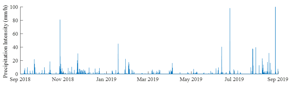
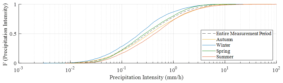
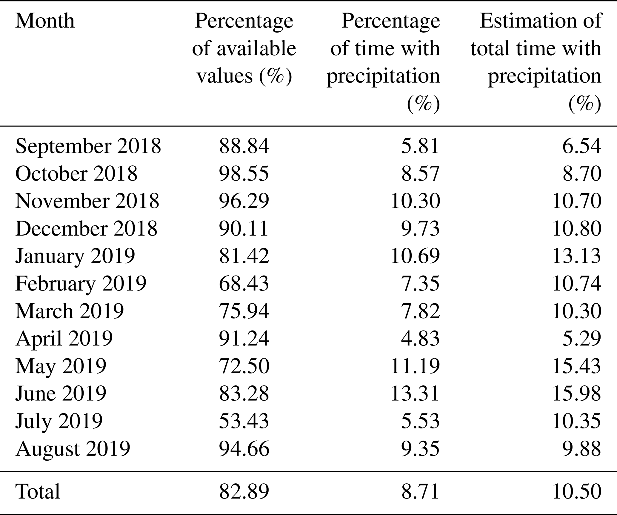
Table 1 presents the percentage of available quality-controlled data for each month and the percentage of the available data in which precipitation was recorded. An estimation of the actual percentage of precipitation can be obtained by assuming that the same proportion of precipitation occurred across the unavailable data. A total of 82.89 % of the data were available during the entire measurement period. Precipitation was recorded in 8.71 % of the available data, giving a yearly precipitation estimate of 10.50 %. Winter had the highest estimation of total time with precipitation with 12.07 %, whilst spring saw the lowest with an estimation of 8.65 %. Including the missing data provides an annual accumulation of 500 mm, which is lower than the 650 mm average annual precipitation reported in Northumberland (WeatherSpark, 2020), indicating that the measurement year was a relatively dry year for the area.
4.2 Precipitation intensity frequency
The average precipitation intensity was recorded every minute. Figure 2 presents its variation across the measurement period, and Fig. 3 presents the cumulative frequency of the recorded intensities. The median precipitation intensity for the measurement period was 0.311 mm h−1.
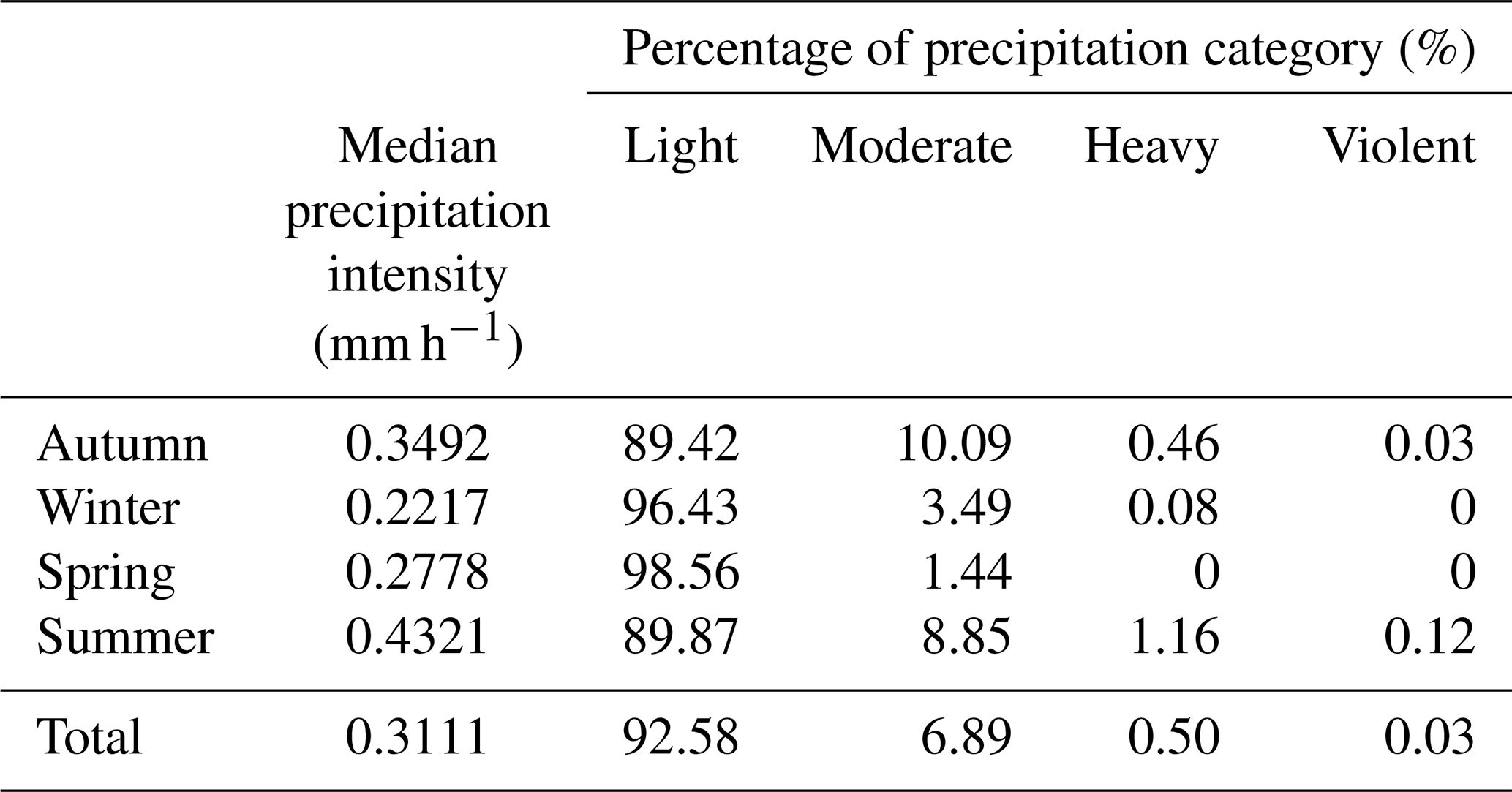
Table 2Precipitation intensity distribution for seasons and intensity categories.
Precipitation is classified according to its intensity with the following categories defined by the Met Office (2007):
-
light – precipitation intensity less than 2.5 mm h−1,
-
moderate – precipitation intensity between 2.5 and 10 mm h−1,
-
heavy – precipitation intensity between 10 and 50 mm h−1,
-
violent – precipitation intensity greater than 50 mm h−1.
The seasonal breakdown of precipitation categories is shown in Table 2. Summer had the highest median precipitation intensity with the highest amount of recorded heavy and violent precipitation. In contrast, winter and spring saw minimal heavy precipitation and no violent precipitation. Light precipitation dominated across the entire measurement period, accounting for 92.58 % of all precipitation. Furthermore, 78.31 % of the recorded minutes had an intensity lower than 1 mm h−1. Moderate precipitation was recorded in 6.89 % of all cases, whilst heavy and violent rain occurred in 0.50 % and 0.03 % cases, respectively. This corresponds to a total of 151 min of heavy precipitation and only 9 min of violent precipitation across the year. This gives a total of 193 min yr−1 of heavy and violent rain once the unavailable data are factored in.
Therefore, a wind turbine in this location would experience less than 3.5 h yr−1 of precipitation with an intensity greater than 10 mm h−1. Without corresponding erosion data, it is not possible to conclude if erosion damage is predominantly caused by heavy and violent precipitation. However, given that erosion can occur within just a few years of installation and assuming that heavy and violent precipitation occurs with the same frequency as found in this dataset, a turbine would experience less than a day of high-intensity rain before erosion occurs. When considering the Springer model, this suggests that erosion damage is not driven solely by heavy and violent precipitation, disagreeing with current research theories (Bech et al., 2018).
4.3 Hydrometeor frequency
Figure 4 presents the number of recorded hydrometeors by type during the data collection period. The hydrometeor type is clearly dominated by rain droplets. “Errors” and “unknown” particles accounted for 17.93 % of the hydrometeors recorded. These may be caused by insects, particles between states or equipment failures and have been ignored in the subsequent analysis, with any records where they were the modal hydrometeor removed. Drizzle and rain droplets make up a combined 98.45 % of all hydrometeors recorded. The number of ice pellets, hail and graupel particles recorded was low, accounting for only 0.49 % of hydrometeors recorded.
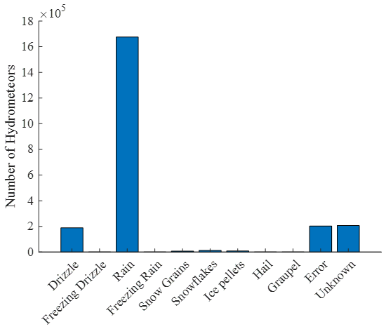
As expected, ice- and snow-based hydrometeors occurred most frequently in winter. Ice pellets, hail and graupel accounted for 0.94 % of the hydrometeors recorded in the season with snow grains and snowflakes accounting for 3.56 %. In contrast, only 0.16 % of hydrometeors recorded in summer were ice pellets or hail, with no graupel, snow grains or snowflakes. Spring and autumn recorded 0.31 % and 0.57 %, respectively, of ice pellets, hail and graupel.
4.4 Hydrometeor velocity
The severity of a hydrometeor impact is governed by its kinetic energy. Whilst the blade speed provides most of the impact velocity, the hydrometeor fall velocity and mass are important. For each minute, the average diameter and velocity was plotted for the modal hydrometeor type. This is presented in Fig. 5.

There is a clear distinction between water particles and snow particles, with snow particles occurring across a wider range of diameters and lower velocities than rain particles. For the few cases where ice pellets were the model hydrometeors, they all occurred to the right of the rain droplet scatter, indicating that they have a lower fall velocity than rain droplets. There were no cases where hail or graupel were the modal hydrometeor, and they were found to be mixed in with rain particles. The presented velocities for water particles are in line with those predicted in models by Gossard et al. (1992) and Brandes et al. (2002). The data presented in the above figure are used in the subsequent analysis to estimate the number of droplets that impact the blade per second and inform lifetime prediction models.
To inform lifetime prediction models, a general equation for an offshore DSD is required. The Best DSD has been reproduced, both seasonally and non-seasonally, with updated constants for the offshore rain data presented. Only data where rain particles were the modal hydrometeor were examined.
5.1 Constant derivation
For each recorded minute, the cumulative function, F, has been evaluated.
Rearranging Eq. (1) gives
Values of n and a for the average precipitation intensity over the minute can therefore be determined by plotting Eq. (4). Figure 6 presents the evaluation of Eq. (4) across a range of precipitation intensities.

Figure 6Evaluation of Eq. (4) for precipitation intensities 0.1058, 1.2708, 4.9865 and 10.2624 mm h−1.
Rearranging Eq. (2) gives
By plotting Eq. (5), the constants A and p can be obtained. Figure 7 evaluates Eq. (5) across the whole dataset.

The constants A and p are determined as 1.0260 and 0.1376, respectively.
Best concluded that the constant n is independent of the precipitation intensity. However, for the data presented, n has dependence on the rain rate. The following relationship applies:
This can be evaluated as
Figure 8 presents the plot of Eq. (7) from which the constants N and q can be obtained.
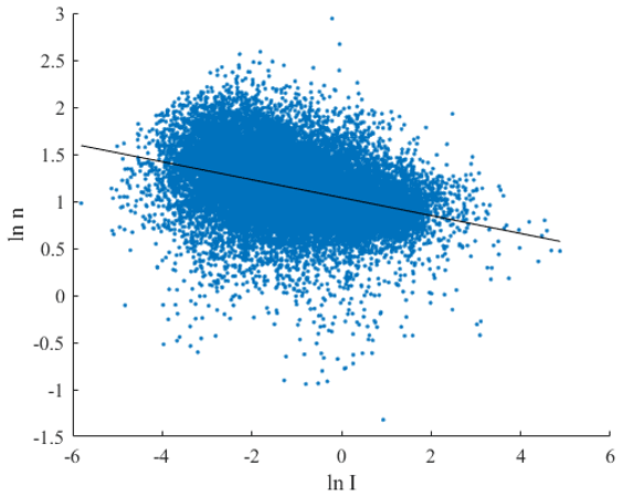
The constants N and q are determined as 2.8264 and −0.0953, respectively. Figure 8 shows substantial scatter in determining these constants. However, as q is small there is only a slight dependence of n on the precipitation rate, and whilst the scatter is likely to introduce some error, it does not have a significant effect on the resulting DSD. Table 3 summarises the constants for the non-seasonal distribution alongside the constants for seasonal DSDs. For detailed modelling and lifetime predictions it may be favourable to use season-dependent DSDs.
Table 3Determined constants for the non-seasonal and seasonal offshore DSDs.

Reproducing Eq. (1) with the derived non-seasonal constants gives a general non-seasonal offshore DSD:
This is presented for various precipitation intensities in Fig. 9.

5.2 Sensitivity analysis
The sensitivity of the constants to the data selected has been evaluated. The following cases have been examined:
-
Low and high precipitation intensity have been individually and collectedly neglected. Precipitation intensities below 0.1 mm h−1 and above 10 mm h−1 were neglected.
-
Precipitation intensities that account for a small number of the recorded intensities have been individually and collectively neglected. These are the bottom 1 % and the top 1 %.
Minutes where the measured precipitation intensity is low generally record fewer droplets than those with higher precipitation intensities. Conversely, a significant number of droplets are generally seen in heavy precipitation. Low- and heavy-intensity rain may, therefore, have a high scatter that could influence the determined constants. Figure 3 presents the cumulative distribution of the recorded precipitation intensities. The bottom and top 1 % of precipitation intensities may also skew the data by providing a point significantly different to the trend. The impact of these conditions on the constants is shown in Table 4.
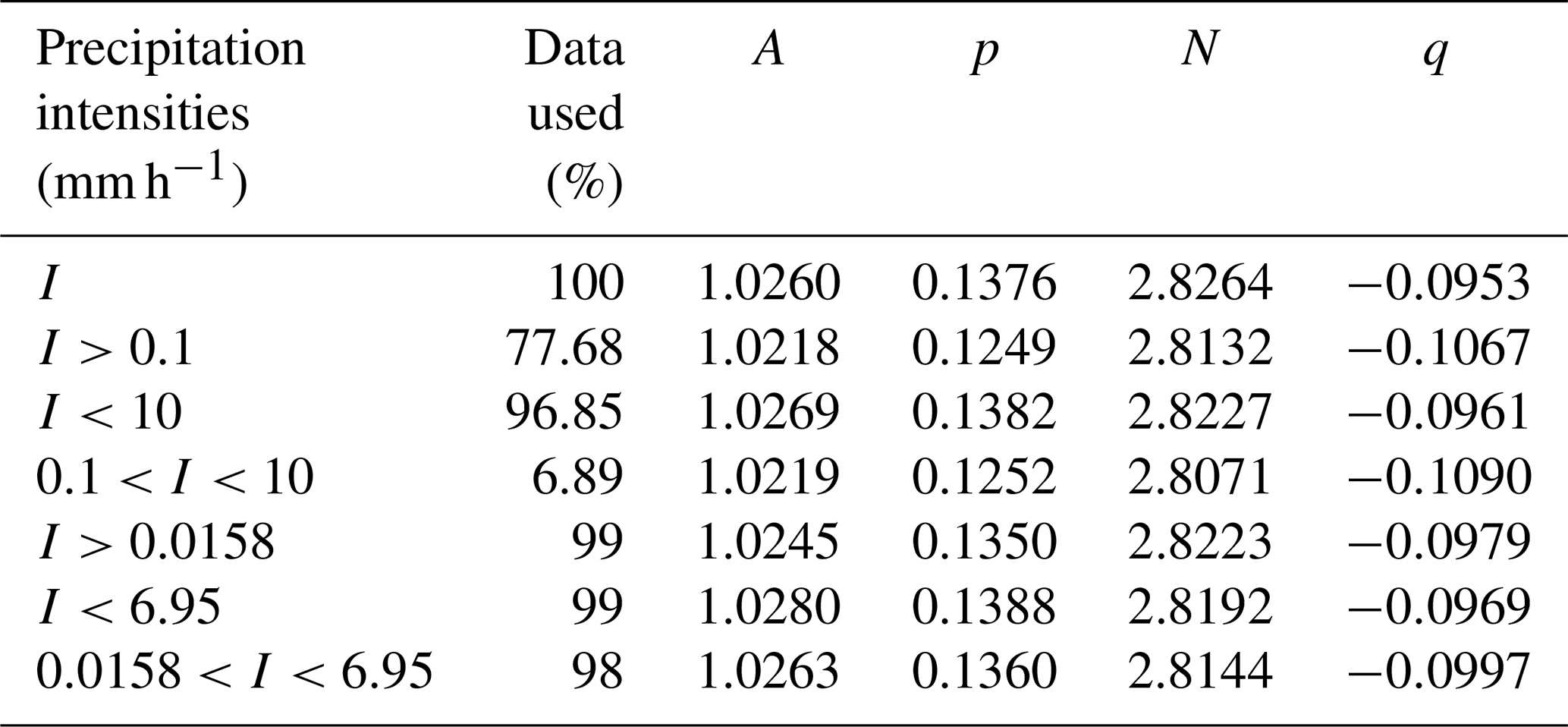
In general, the constants are consistent across all the examined cases. The constant p is the most sensitive to the data included. Neglecting low precipitation intensities reduces its value, whilst neglecting higher intensities increases its value. Removing precipitation intensities below 0.1 mm h−1 has the greatest effect on the constants. However, ignoring these intensities loses 22.32 % of the data available. It can be concluded that the proposed constants are acceptable.
5.3 Comparison to Best DSD
The general offshore DSD has been compared to the Best DSD at various precipitation intensities in Fig. 10. The precipitation intensities 0.1, 1, 2.5, 5, 10 and 20 mm h−1 were selected to enable comparison of the two DSDs across a range of intensities. To account for variability in the recorded results, minutes which recorded an intensity within ±5 % of the selected intensity were included. For each data group, the intensities were averaged and the offshore DSD and Best DSD for the average intensity were plotted against them.

Figure 10Comparison between the offshore DSD and the Best DSD at precipitation intensities (a) 0.10005, (b) 0.99612, (c) 2.501, (d) 4.9818, (e) 10.0194 and (f) 19.9687 mm h−1.
Figure 10 reveals that the Best DSD significantly overestimates the diameter of droplets. This is particularly true at the higher precipitation intensities. The goodness of fit of the offshore and Best DSDs has been evaluated across the range of precipitation intensities in Fig. 11. The offshore DSD aligns well with the raw data and possesses a high coefficient of determination (R2) across the precipitation intensity range. The slight reduction in R2 at higher intensities can be attributed to the reduced amount of heavy and violent precipitation recorded. The coefficient of determination of the Best DSD reduces significantly as the precipitation intensity increases.
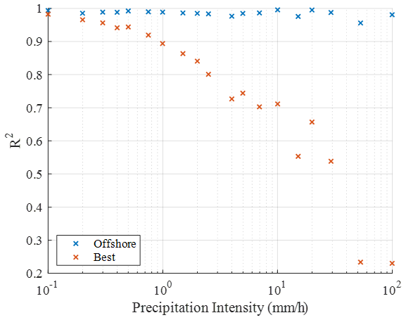
Figure 11Coefficient of determination of the offshore DSD and the Best DSD across a range of precipitation intensities.
5.4 Limitations
The offshore DSD presented has two main limitations. Firstly, the presented measurement period may be a limiting factor. As the disdrometer continues to collect data, the DSD can be further refined. Secondly, data have only been collected at one point. Offshore DSDs may vary from location to location. To address this, a disdrometer has been positioned at ORE Catapult's Levenmouth offshore demonstration turbine for future comparison and validation.
The implications of the offshore DSD have been assessed using the Springer model, which is used by Eisenberg et al. (2018) to predict a protection solution's in situ lifetime from leading edge erosion. The model uses the median droplet diameter for a given rain rate to determine the number of impacts to failure, Nic, and the number of impacts on the blade per square metre per second, . The number of impacts to failure is found from
where Sec is the effective strength of the protection system found from rain erosion test results and is the pressure at the interface between the droplet and protection system and is a function of the droplet diameter and the properties of the system relative to the substrate it is applied on. The number of impacts on the blade per square metre per second is given as
where q is the number of droplets in a cubic metre of air; Vs is the velocity of the drop impact; and β is the impingement efficiency of the droplets, which is dependent on the aerofoil geometry and droplet diameter. The number of droplets per cubic metre is found from geometry and is presented by Springer et al. (1974) as
where Vt is the terminal velocity of the droplets.
The rate of damage, , from a given precipitation intensity is found from
The analysis presented here has shown that the Best DSD currently used in the Springer model overestimates the size of impinging offshore droplets.
The exact number of impacts to failure is dependent on the protection system and substrate used. For a commercial erosion-resistant polyurethane coating system, the offshore DSD has been applied to the above equations, and the relative effect on leading edge erosion prediction of the DSD in relation to the Best DSD is presented in Fig. 12.

Figure 12Percentage change in leading edge erosion damage values from implementing the offshore DSD relative to implementing the Best DSD.
The smaller median droplet diameter for precipitation intensities above 0.15 mm h−1 requires a greater number of impacts to reach initiation. However, the equations show that there are a far greater number of droplet impacts per second, giving a higher damage rate for precipitation intensities, with the difference becoming substantial at the higher intensities. The impact of this is dependent on the site conditions and frequency of precipitation intensities. However, for the dataset presented here and the above material properties, the implementation of the offshore DSD causes the Springer model to predict a 23.7 % reduction in lifetime in comparison to when the Best DSD is implemented. As a result, employing the Best DSD in leading edge erosion prediction models underestimates the severity of the offshore environment in terms of leading edge erosion. Therefore, the lifetime of protection systems installed offshore is greatly overestimated, resulting in earlier than expected maintenance and ultimately a higher cost of energy.
This dataset can be used to help to inform the lifetime of leading edge erosion protection systems installed offshore, helping to ensure maintenance is conducted early and further leading edge erosion can be combatted. The dataset can also be used to inform droplet impact models and rain erosion testing with the greater understanding of the environment facilitating the development of improved protection systems.
DSDs are important in predicting and modelling leading edge erosion. Currently, there is a lack of an offshore dataset and the industry uses onshore distributions in lifetime predictions. In this work, a disdrometer has been positioned 3 nautical miles (5.56 km) offshore to collect and characterise the offshore precipitation environment and to provide an offshore DSD for lifetime prediction models.
Heavy and violent precipitation was rare in the measurement period, accounting for less than 3.5 h of precipitation across the year. Therefore, erosion damage is not likely to be driven exclusively by heavy and violent precipitation. Rain was the most frequently occurring hydrometeor, whereas snow, ice and hail particles were scarce. A clear distinction was visible in the diameter–velocity plots for each hydrometeor, with snow particles occurring across a wider range of diameters and lower average velocities. The majority of raindrops observed had a diameter below 2 mm.
A general offshore DSD has been presented. The raw data were compared to the presented DSD and the most widely used DSD proposed by Best. A statistical R2 analysis found that the offshore DSD aligned well with the data, whereas the Best DSD significantly overestimated the diameters of droplets. The implication of the offshore DSD was evaluated with the Springer model, where it was found the inaccuracies in the Best DSD greatly underestimate the severity of the offshore environment in terms of leading edge erosion. As a result, the Best DSD is not a suitable distribution to use in lifetime prediction models for protection systems positioned offshore, and therefore predictions determined using it are unlikely to be accurate.
The results presented address the lack of an offshore dataset and provide a general offshore DSD that can be used to inform lifetime prediction models for the offshore environment. A disdrometer has been placed at ORE Catapult's Levenmouth offshore wind turbine to provide further information about the precipitation environment and validate the presented DSD. The offshore dataset can be used to improve prediction and modelling techniques, helping to inform the design of new protection solutions and to combat leading edge erosion whilst reducing lost energy production and unexpected turbine downtime.
Please contact the corresponding author.
RH had the lead on paper writing and data analysis and derived conclusions. KD and PH were responsible for installing and setting up the disdrometers. KD and CW supervised the research.
The authors declare that they have no conflict of interest.
This article is part of the special issue “WindEurope Offshore 2019”. It is a result of the WindEurope Offshore 2019, Copenhagen, Denmark, 26–28 November 2019.
This work was supported by the Engineering and Physical Sciences Research Council through the EPSRC Centre for Doctoral Training in Composites Manufacture, project partner the Offshore Renewable Energy Catapult, https://ore.catapult.org.uk (last access: 26 October 2020), and the EPSRC Future Composites Manufacturing Hub. The authors would also like to thank the Wind Blade Research Hub for their support in the delivery of this paper.
This research has been supported by the EPSRC Centre for Doctoral Training in Composites Manufacture (grant no. EP/K50323X/1) and the EPSRC Future Composites Manufacturing Hub (grant no. EP/P006701/1).
This paper was edited by Ignacio Marti Perez and reviewed by two anonymous referees.
Agnew, J.: Final report on the operation of a Campbell Scientific PWS100 present weather sensor at Chilbolton Observatory, Science & Technology Facilities Council, Swindon, UK, 2013.
Bech, J. I., Hasager, C. B., and Bak, C.: Extending the life of wind turbine blade leading edges by reducing the tip speed during extreme precipitation events, Wind Energ. Sci., 3, 729–748, https://doi.org/10.5194/wes-3-729-2018, 2018.
Best, A. C.: The size distribution of raindrops, Q. J. Roy. Meteorol. Soc., 76, 16–36, https://doi.org/10.1002/qj.49707632704, 1950.
Brandes, E. A., Zhang, G., and Vivekanandan, J.: Experiments in Rainfall Estimation with a Polarimetric Radar in a Subtropical Environment, J. Appl. Meterol., 41, 674–685, 2002.
Chen, B., Wang, J., and Gong, D.: Raindrop Size Distribution in a Midlatitude Continental Squall Line Measured by Thies Optical Disdrometers over East China, J. Appl. Meteorol. Clim., 55, 621–634, https://doi.org/10.1175/JAMC-D-15-0127.1, 2016.
Doagou-Rad, S. and Mishnaevsky, L.: Rain erosion of wind turbine blades: computational analysis of parameters controlling the surface degradation, Meccanica, 55, 725–743, https://doi.org/10.1007/s11012-019-01089-x, 2020.
Eisenberg, D., Laustsen, S., and Stege, J.: Wind turbine blade coating leading edge rain erosion model: Development and validation, Wind Energy, 21, 942–951, https://doi.org/10.1002/we.2200, 2018.
Finans: Siemens sets billions: Ørsted must repair hundreds of turbines, windAction, available at: http://www.windaction.org/posts/47883-siemens-sets-billions-orsted-must-repair-hundreds-of- (last access: 21 October 2019), 2018.
Gossard, E. E., Strauch, R. G., Welsh, D. C., and Matrosov, S. Y.: Cloud Layers, Particle Identification and Rain-Rate Profiles from ZRVf Measurements by Clear-Air Doppler Radars, J. Atmos. Ocean. Tech., 9, 108–119, 1992.
Hasager, C., Vejen, F., Bech, J. I., Skrzypiński, W. R., Tilg, A.-M., and Nielsen, M.: Assessment of the rain and wind climate with focus on wind turbine blade leading edge erosion rate and expected lifetime in Danish Seas, Renew. Energy, 149, 91–102, https://doi.org/10.1016/j.renene.2019.12.043, 2020.
Jennings, K. S., Winchell, T. S., Livneh, B., and Molotch, N. P.: Spatial variation of the rain-snow temperature threshold across the Northern Hemisphere, Nat. Commun., 9, 1–9, https://doi.org/10.1038/s41467-018-03629-7, 2018.
Johannsen, L. L., Zambon, N., Strauss, P., Dostal, T., Zumr, D., Cochrane, T. A., Blöschl, G., Klik, A., Lolk, L., Zambon, N., Strauss, P., Dostal, T., Zumr, D., Cochrane, T. A., Blöschl, G., and Comparison, A. K.: Comparison of three types of laser optical disdrometers under natural rainfall conditions, Hydrolog. Sci. J., 65, 524–535, https://doi.org/10.1080/02626667.2019.1709641, 2020.
Kathiravelu, G., Lucke, T., and Nichols, P.: Rain Drop Measurement Techniques: A Review, Water, 8, 29, https://doi.org/10.3390/w8010029, 2016.
Keegan, M. H., Nash, D. H., and Stack, M. M.: Modelling Rain Drop Impact of Offshore Wind Turbine Blades, in: ASME Turbo Expo 2012: Turbine Technical Conference and Exposition, American Society of Mechanical Engineers, Copenhagen, Denmark, 887–898, 2012.
Met Office: Fact sheet No. 3 – Water in the atmosphere, Devon, UK, 2007.
Montero-Martínez, G., Torres-Pérez, E. F. and García-García, F.: A comparison of two optical precipitation sensors with different operating principles: The PWS100 and the OAP-2DP, Atmos. Res., 178–179, 550–558, https://doi.org/10.1016/j.atmosres.2016.05.007, 2016.
Slot, H. M., Gelinck, E. R. M., Rentrop, C., and van der Heide, E.: Leading edge erosion of coated wind turbine blades: Review of coating life models, Renew. Energy, 80, 837–848, https://doi.org/10.1016/j.renene.2015.02.036, 2015.
Sommerville, D. R. and Matta, J. E.: A method for determinging droplet size distributions and evaporational losses using paper impaction cards and dye trackers, Chemical Research Development & Engineering Center, Maryland, USA, 1990.
Springer, G. S., Yang, C.-I., and Larsen, P. S.: Analysis of Rain Erosion of Coated Materials, J. Compos. Mater., 8, 229–252, https://doi.org/10.1177/002199837400800302, 1974.
Vejen, F., Tilg, A., Nielsen, M., and Hasager, C.: D1.2 Precipitation statistics for selected wind farms, Innovationsfonden, Rosekilde, 2018.
WeatherSpark: Average Weather in Alnwick, Northumberland, available at: https://weatherspark.com/y/42298/Average-Weather-in-Alnwick-United-Kingdom-Year-Round, last access: 1 June 2020.
- Abstract
- Introduction
- The Best distribution
- Offshore measurement technique
- The offshore dataset
- Offshore rain distribution
- Impact of DSD on leading edge erosion lifetime prediction
- Conclusions
- Data availability
- Author contributions
- Competing interests
- Special issue statement
- Acknowledgements
- Financial support
- Review statement
- References