Full-scale deformation measurements of a wind turbine rotor in comparison with aeroelastic simulations

The measurement of deformation and vibration of wind turbine rotor blades in field tests is a substantial part of the validation of aeroelastic codes. This becomes highly important for modern rotors as the rotor size increases, which comes along with structural changes, resulting in very high flexibility and coupling between different vibration modes. However, performing full-scale field measurements for rotor blade deformation is not trivial and requires high temporal and spatial resolution. A promising deformation measurement technique is based on an optical method called digital image correlation (DIC). Recently, DIC measurements on a Siemens Gamesa SWT-4.0-130 test turbine were performed on the tip of all blades in combination with marker tracking at the hub for the first time with synchronised measurement of the inflow conditions by a ground-based lidar. As the turbine was additionally equipped with strain gauges in the blade root of all blades, the DIC results can be directly compared to the actual prevailing loads to validate the measurement method. In the end, an example for a comparison of the measured deformations and torsion with aeroelastic simulations is shown in the time and frequency domain. All in all, DIC shows very good agreement with comparative measurements and simulations, which shows that it is a suitable method for measurement of deformation and torsion of multi-megawatt wind turbine rotor blades.

1 Introduction

The increasing demand for a reduction in levelised cost of electricity (LCOE) of wind turbines leads to substantial changes in the design, operation, and reliability of wind turbines and plants (Dykes et al., 2019). Changes in the design of the rotor are a leading driver for the reduction in LCOE for onshore turbines: by increasing the rotor size (Wiser et al., 2016). This is only possible by realising crucial changes in the structural design of wind turbine blades as the mass of the blades naturally scales with the volume and thus with the cube of the rotor blade length, whereas the energy capture scales only with the area of the rotor and thus with the square of the rotor blade length (the so-called “square–cube law”). The need for a reduction in mass per rotor blade length is realised by applying methods for the reduction in the volume, like aeroelastic tailoring. Thus, the knowledge of the aeroelastic behaviour is one of the biggest challenges in today's and especially in future wind turbine engineering (Veers et al., 2019).

Along with this comes the need for experimental validation of aeroelastic modelling. Until today, the load of wind turbine rotor blades is usually measured with strain gauges in edgewise and flap-wise directions; however measuring the rotor blade deformation and torsion is still a challenge. Optical measurement methods can make a contribution to this. In the past, several optical measurement methods were successfully applied on full-scale wind turbines for the determination of rotor blade deflections during operation (Schmidt Paulsen et al., 2009; Ozbek and Rixen, 2013; Grosse-Schwiep et al., 2014; Lutzmann et al., 2016).

For the direct measurement of rotor blade deformation (in-plane as well as out-of-plane) and torsion of full-scale wind turbines, only a few suitable measurement methods exist, which are shortly introduced. In the past years, Siemens Gamesa developed an in-house photographic method for the detection of these variables (Mayda et al., 2013). For this method, a camera is installed in the blade root region of a rotor blade, facing the blade tip. At different radial positions, optical markers are installed upright relative to the pressure side, and on these sections, the deformation and twist can be detected. Another method called BladeVision was developed by SSB Wind Systems (Nidec SSB Wind Systems GmbH, 2020). For this method, a camera is installed in the inner side of the blade root region of the blade. Reflectors are also installed inside at different radial positions and are monitored by the camera for the determination of deformation and twist at those positions. Another method was developed by ForWind, Institute of Turbomachinery and Fluid Dynamics, Leibniz Universität Hannover. This method is based on digital image correlation (DIC). For this method, a stereo camera system is installed in the area in front of the turbine, and random speckle patterns are applied on the blades' pressure side. On those sections where the pattern has been applied, the deformation and torsion of the rotor blade can be detected. All of the three optical methods described above have advantages and disadvantages. As an example, DIC is sensitive to the changing weather conditions outside, but it can be easily installed on the blade compared to the other two methods.

Before DIC was applied on full-scale wind turbines, the feasibility and accuracy were determined on a scaled wind turbine model (Winstroth and Seume, 2014a) as well as within a fully virtual experiment (Winstroth and Seume, 2014b). Afterwards, the feasibility of this measurement method at full scale on a 3.2 MW wind turbine was proven (Winstroth and Seume, 2015). Wu et al. (2019) have demonstrated the applicability of the method by successfully applying DIC on a 5 kW wind turbine to obtain the full-field displacement and strain of the rotor blades. A comparison of out-of-plane deformations (measured with DIC) with aeroelastic simulations for a short time series of 30 s was also done (Winstroth et al., 2014). The results show that such a comparison is not trivial as the selection of time series can have a significant influence on the results when the time series is very short and the simulations are based on statistical wind conditions.

The next step is now the conduction of a longer time series and a comparison with high-fidelity aeroelastic simulations, which includes both deflections and torsion. This is part of this paper in order to prove that DIC can be a beneficial tool for the validation of aeroelastic codes. Additionally, the DIC results are compared to load measurements in the frequency domain to validate this technique with conventional measurement methods. A 5 min time series of DIC measurements is used to show the feasibility and thus the potential of validating aeroelastic codes based on DIC measurements.

Firstly, the experimental set-up for the execution of optical measurements on a full-scale wind turbine is described. The speckles for DIC were applied in the tip region on all three blades. For the detection of the movement and rotation of the hub, three big speckles were applied on the hub itself. The hub movement is later on used for the determination of in-plane (IP) deformation, out-of-plane (OoP) deformation, and torsion out of the DIC signal. Afterwards, the functionality of the two optical methods applied, DIC and marker tracking, is briefly explained. Measurement results are shown and compared to strain gauge signals at the blade root for a qualitative experimental validation of the optical method. For a rough validation of the combined rotor blade pitch and torsion angle, the DIC signal is compared to the pitch signal of the turbine. This can only prove a trend as there is no additional measurement technique installed for the determination of rotor blade torsion. Results of a power spectral density (PSD) estimation with Welch's method of the signals are shown and compared to the natural eigenfrequencies that are expected to occur from numerical computations. Finally, one time series of DIC measurements is compared to aeroelastic simulations of the turbine to demonstrate a way of experimentally validating rotor blade deformation and torsion based on DIC measurements.

2 Experimental set-up

The general measurement set-up for the execution of DIC measurements on wind turbines is shown in Fig. 1. Different radial positions of the blades can be equipped with self-adhesive foils to build a speckle pattern on the rotor blade. The deformation can be captured in those areas where the speckles are applied, so this could be done along the whole length of the blade. A stereo camera system is placed in the area upstream of the turbine to monitor the whole rotor during operation.

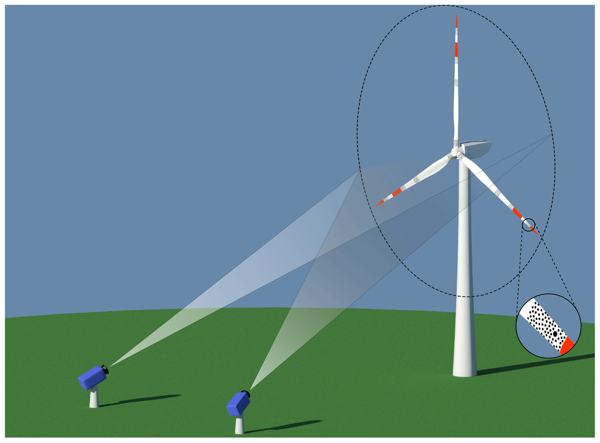
Figure 1 Schematic of a camera set-up in front of a full-scale wind turbine. The magnified cut-out near the blade tip shows the random black-and-white pattern on the pressure side (Winstroth and Seume, 2015).

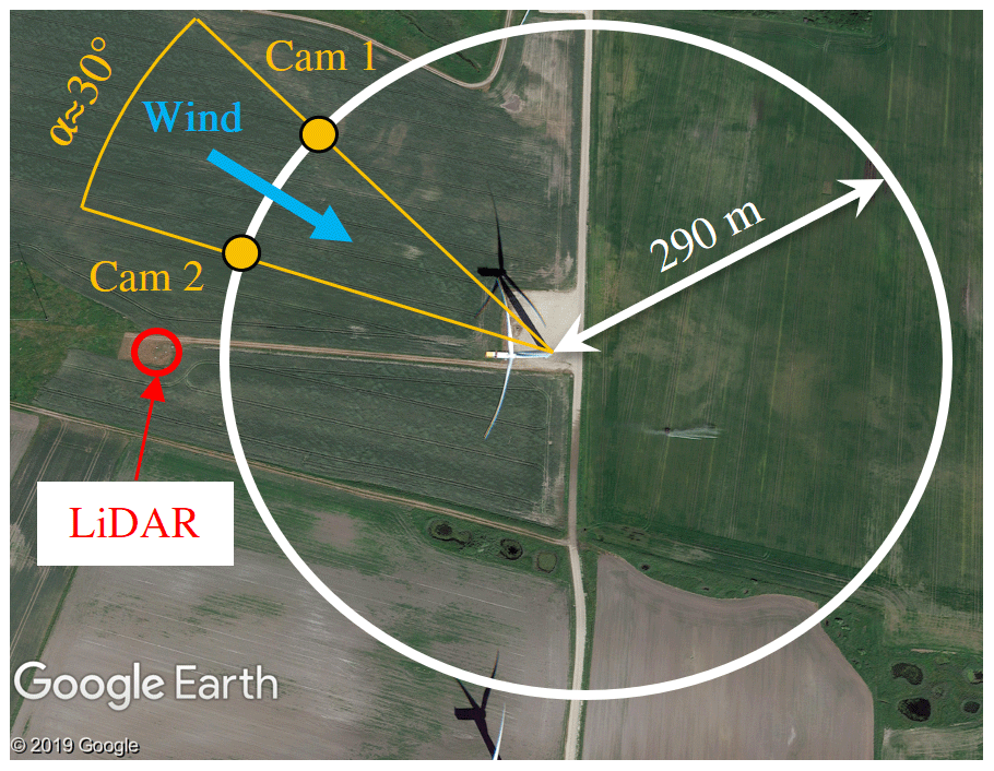
Figure 2 Experimental set-up at the Høvsøre wind turbine test site.

In this measurement campaign, a Siemens Gamesa SWT-4.0-130 test turbine located at the DTU wind turbine test centre in Høvsøre, in Denmark, was equipped with a speckle pattern for DIC measurements in the tip region of all three blades. The cameras have a resolution of 25 MP and take pictures simultaneously with a frame rate of 30 frames per second (fps). Each camera is connected via CameraLink to a measurement computer to store the pictures directly on the hard drive. Due to the high data rate of 750 MBps per camera, the maximum measurement duration with the current set-up is limited to 10 min. Usually it is not the hard drive which limits the measurement duration but rather the change in weather and ambient lighting conditions.

Figure 3 Random speckle pattern for the application of DIC on the blade tips.

Figure 4 Three big dots on the nacelle for the application of marker tracking on the hub.

Each camera is equipped with a lens of a 58 mm fixed focal length. In order to monitor the full rotor diameter of 130 m, the cameras are placed 290 m away from the foundation of the turbine (see Fig. 2). The cameras are positioned in a 30^∘ stereo angle configuration relative to the wind turbine. The wind direction should remain constant in the region between the two cameras to have an optimal angle of sight for both cameras. The turbine is allowed to yaw within this region, but if the angle between the rotor plane and the camera becomes too sharp, the speckles cannot be identified well enough. The wind speed and direction at 10 different heights throughout the full extension of the rotor are measured at a sampling frequency of 1 Hz with a lidar located at a distance of 2.5 rotor diameters in front of the turbine in order to be able to assess shear and veer properly. Furthermore, the atmospheric temperature, pressure, and humidity are also logged to estimate the air density.

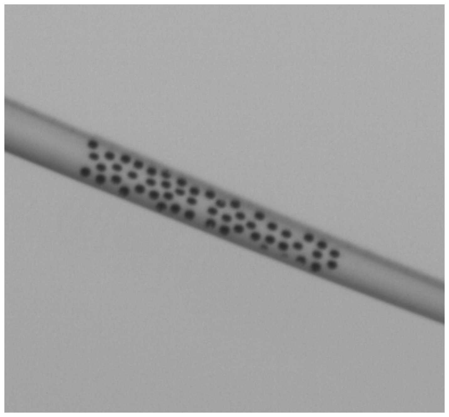
The speckles were applied on the pressure side of the blades from a lift in the range of 55 to 60 m measured from the blade root (see Fig. 3). The speckle pattern needs to be different for all blades as DIC finds a unique greyscale signature for every measurement point. Per blade, approximately 50 speckles with a diameter of 20 cm were applied that build a random black-and-white speckle pattern. The hub is used to define the rotor plane and the rotational axis. In this case, three single dots with a diameter of 70 cm were applied, which are analysed with a marker-tracking algorithm (see Fig. 4).

The turbine is instrumented with strain gauges in the root of all three blades, and furthermore, the following operational parameters are logged with a 25 Hz sampling frequency: pitch, rotor speed, and power. This is useful for a comparison of DIC with conventional measurement methods in the field.

DIC is typically used in laboratory environments with constant illumination. As this set-up is now applied in the field, where the sun is the only suitable light source, a great deal of experience is required to perform a successful measurement under these conditions. The movement of clouds makes it a challenge to find a time slot which is longer than 5 min where illumination conditions remain constant.

The difference between DIC and marker tracking is that with marker tracking the single dots are tracked and not the full-field area between them. The advantage is that the position of the single markers is clearly defined, which comes along with the disadvantage of a higher inaccuracy. Out of this set-up, the track of three single dots is extracted to define the rotor axis and the rotor plane. The blade tip regions are evaluated with the DIC algorithm and result in an areal information of the whole speckle pattern area, defined by the track of approximately 1000 points per blade tip.

3 Digital image correlation

In general, the term digital image correlation describes an optical measurement method which is part of photogrammetry that acquires images to calculate the full-field shape, deformation, and/or motion measurements of certain objects (Sutton et al., 2009). This process consists of the digital image acquisition itself, the storage, and the performance of an image analysis to obtain motion and deformation out of the images. In this part, the analysis is briefly described. The reader is referred to Sutton et al. (2009) for a more detailed description of the analysis methods.

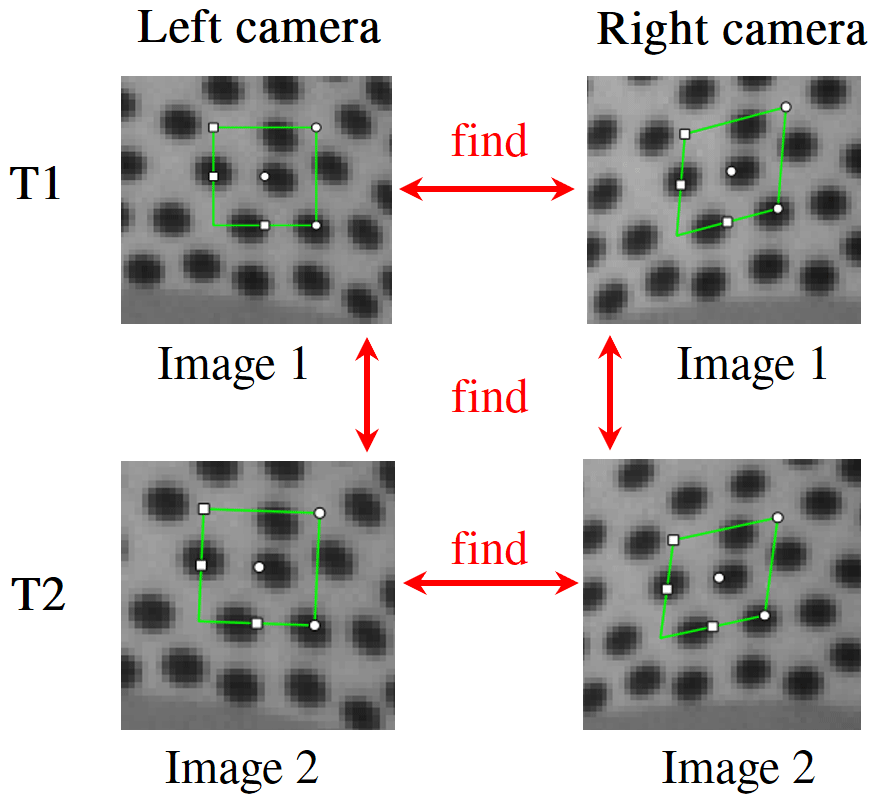
Figure 5 The DIC algorithm finds points by tracking the greyscale signature of the subset in every picture.

The DIC algorithm applies several different analysis methods. It all starts with the recognition of the same points in all images. This process is shown in Fig. 5 for one measurement point.

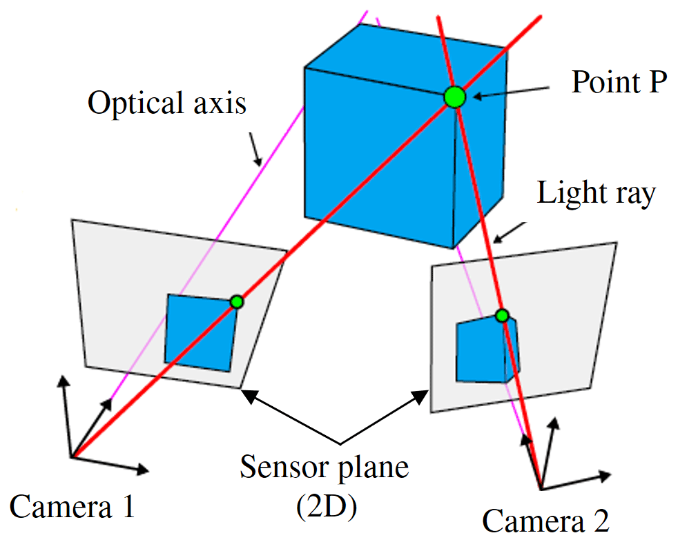
Figure 6 The position of the point P in 3D is calculated by the position of the two cameras relative to the wind turbine and the individual position of the measurement point in the left and right picture.

The white dot in the middle of the green rectangle is the actual measurement point, which is defined by the greyscale signature F of the neighbouring pixels that form a subset (green rectangle). The greyscale signature is defined as the distribution of greyscale values of all pixels in the defined subset and is a function of the local coordinates F=f(x), where x is defined as a two-dimensional vector x=(x y). At the time T1, the measurement point in image 1 of the left camera (usually the reference picture) is defined and is found in the following pictures as the greyscale signature G, which is a function of the local coordinates and a displacement term p, resulting in $G=f(\mathit{x},\mathit{p})$. The greyscale value of a certain subset is obtained by building the sum of greyscale values of all neighboured pixels in the subset in the form of ∑F and ∑G.

The reference subset is defined in the reference image 1 of the left camera and is usually rectangular. To find a similar (or in a perfect case the same) greyscale in the following pictures of the same camera, a shape function needs to be introduced as the subset might not have the same shape. This shape function ξ(x,p) is used to transform pixel coordinates in the reference subset into coordinates in the image after deformation. This results in a correlation function χ that is dependent on the shape of the subset as follows:

$$\begin{array}{}\text{(1)}& {\mathit{\chi }}^{\mathrm{2}}\left(\mathit{p}\right)=\sum \left(G\right(\mathit{\xi }(\mathit{x},\mathit{p}))-F(\mathit{x}){)}^{\mathrm{2}}.\end{array}$$

The search for the best match between F and G is driven by computing the value of χ by iteratively updating p. For an affine transformation, ξ can be defined as

$$\begin{array}{}\text{(2)}& \mathit{\xi }(\mathit{x},\mathit{p})=\begin{array}{c}\left[\begin{array}{l}{p}_{\mathrm{0}}\\ p_{\mathrm{1}}\end{array}\right]\end{array}+\begin{array}{c}\left[\begin{array}{lr}\mathrm{1}+p_{\mathrm{2}}& p_{\mathrm{3}}\\ p_{\mathrm{4}}& \mathrm{1}+p_{\mathrm{5}}\end{array}\right]\end{array}x,\end{array}$$

where six components of p are introduced. p₀ and p₁ define the translational displacement of the subset in the picture, whereas p₂, p₃, p₄, and p₅ change the rotation, compression, and shear of the subset shape.

Figure 7 Measurement points plotted on the rotor blade.

Different solving algorithms exist to find the optimal value of χ, where for DIC, all are based on the normalised cross-correlation (NCC) criterion ${\mathit{\chi }}_{\mathrm{NCC}}^{\mathrm{2}}$ that is actually the origin of the term correlation in DIC:

$$\begin{array}{}\text{(3)}& {\mathit{\chi }}_{\mathrm{NCC}}^{\mathrm{2}}={\displaystyle \frac{\sum FG}{\sqrt{\sum F^{\mathrm{2}}\sum G^{\mathrm{2}}}}}.\end{array}$$

The correlation criterion χ is bounded in the interval [0, 1], where 1 represents a perfect match. Usually, the maximum match is found under application of the Levenberg–Marquardt algorithm (Levenberg, 1944; Marquardt, 1963).

This criterion is extended to account for lighting offsets, scales relative to the reference picture, and results in the zero-mean normalised sum of squared difference (ZNSSD) criterion ${\mathit{\chi }}_{\mathrm{ZNSSD}}^{\mathrm{2}}$:

$$\begin{array}{}\text{(4)}& {\mathit{\chi }}_{\mathrm{ZNSSD}}^{\mathrm{2}}=\sum {\left(\left({\displaystyle \frac{\sum \overline{F_i}\overline{G_i}}{\sum {\overline{G_i}}^{\mathrm{2}}}}{G}_i-\overline{G}{\displaystyle \frac{\sum \overline{F_i}\overline{G_i}}{\sum {\overline{G_i}}^{\mathrm{2}}}}\right)-F_i+\overline{F}\right)}^{\mathrm{2}}.\end{array}$$

$\overline{F_i}$ and $\overline{G_i}$ are defined as the difference of the current value to the mean value, resulting in $\overline{F_i}=F_i-\overline{F}$ and $\overline{G_i}=G_i-\overline{G}$.

The stereo matching between the left and the right camera is done under application of a plane-to-plane homography matrix. This homography matrix relates image coordinates to coordinates on a plane in space. As both cameras' coordinates in the world are known after the external calibration, image coordinates of the left camera can be related to image coordinates of the right camera through a homographic transformation, more commonly referred to as rectification in computer vision.

Figure 8 Measurement points plotted in 3D, not aligned to the rotor coordinate system.

To achieve the maximum geometrical resolution, sub-pixel interpolation is applied in the matching algorithm. The sub-pixels are interpolated by a continuous eight-tap spline.

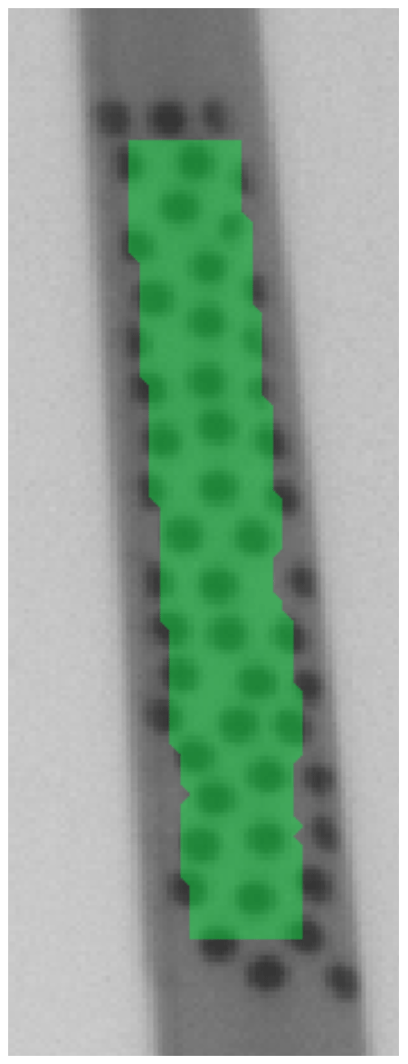
The result of the application of the DIC algorithm with the software Vic3D by Correlated Solutions, Inc. (Correlated Solutions, Inc., 2020) can be seen in Fig. 7. The measurement points that are obtained are highlighted in green. It can be seen that the algorithm did not converge in the outer region, which is due to the definition of the subset size.

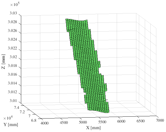
This data set can be directly imported in MATLAB, the result of which is shown in Fig. 8. The measurement points are not aligned to the rotor coordinate system at this evaluation step.

Figure 9 Evaluation of DIC and point-tracking method for determination of rotor blade deformation and torsion.

The marker-tracking algorithm also applies a sub-pixel interpolation to find the right match of the marker in all images; however there is no definition of subsets as the marker itself is directly tracked. This guarantees that the exact position of the markers will be calculated but results in a less accurate signal compared to the areal DIC method. This requires the application of a low-pass filter to the hub track. As the movement of the nacelle is slow compared to the movement of the blade tips, this method is still suitable for the detection of the hub track. The areal DIC tracks are not filtered and thus can be used directly for evaluation.

4 Determination of rotor blade deformation and torsion

The evaluation of the optical measurement is split into five main parts, which are shown in Fig. 9. The first part (1) is the detection of the positions of the speckle pattern out of the pictures, i.e. the application of a DIC algorithm to the image series. This is done with the commercial software Vic3D from Correlated Solutions, Inc. (Correlated Solutions, Inc., 2020). The software can track the position of the speckle regions even under a rotating movement of the object. In a second step (2), the movement of the hub is determined by tracking the position of the three markers on the hub itself with a marker-tracking algorithm, which is also included in Vic3D. This defines the rotor axis as well as the rotor plane (3), which is necessary for the next step. In a fourth step (4), the positions are classified into in-plane (IP) deformation and out-of-plane (OoP) deformation by removing the hub movement from DIC data. The OoP deformation can be further used to calculate the torsional deformation of the rotor blade (5).

Figure 10 Track of one measurement point of DIC without alignment.

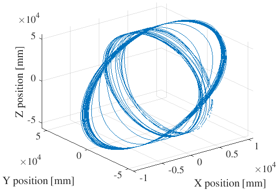
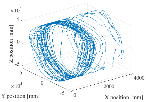
The output of DIC is full-field information of the position of the surface of the rotor blades' pressure side in 3D. An example for the direct output of one DIC measurement point is shown in Fig. 10. The coordinate system is not aligned; thus the measurement point rotates around an undefined rotational axis. A change in the yaw position of the rotor can be clearly seen in this track. To define the deformation in OoP and IP, the rotor plane needs to be aligned with the rotor coordinate system. To define the position and orientation of the rotational axis, which is step (3), the tracks of the markers on the hub are used. This is done in three steps:

• i.

  translational alignment of the hub centre to the origin of the coordinate system
  → elimination of translational movement

• ii.

  rotational alignment of the normal vector on the hub to the x axis of the coordinate system
  → elimination of yaw and roll angle

• iii.

  rotational alignment of the measurement point around the rotational axis
  → elimination of azimuth angle.

The translational displacement (i) of the rotational axis is found by determining the centre of the position of the three markers. The markers are not perfectly positioned at the same distance to the rotational axis, which results in a remaining rotational radius of approximately 20 mm, which can safely be considered negligible. The translational displacement of the rotational axis is determined for every time step and removed from the original DIC data.

The rotational misalignment (ii) between the normal vector of the rotor plane and the x axis in the coordinate system is determined. This results in two angles which are removed from the DIC data for every time step: yaw and roll angle. The result of this can be seen in Fig. 11. What remains is the rotation around the x axis, which is defined as the azimuth angle.

Figure 11 Track of one measurement point of DIC aligned to the rotor plane.

In a third step, the azimuth angle needs to be removed (iii). For this, the reference measurement point of the centre of rotation is aligned with the z axis. The azimuth angle is determined as the rotational offset around the x axis between the actual measurement point and the reference point. Now that the azimuth angle is determined, it can be removed from the DIC signal that is aligned with the rotor plane.

The displacement that remains in the DIC measurement points is defined as follows:

• movement in x direction → out-of-plane (OoP) deformation

• movement in y direction → in-plane (IP) deformation

• movement in z direction → radial deformation.

The radial deformation is affected by the radial displacement of the hub marker centre to the actual rotational axis remaining in the measurement data.

Figure 12 shows a view of the rotor blade chord of length c in relative position to the rotor plane. The angle β defines the rotation around the vertical axis of the rotor blade and is a combination of pitch and torsion angle. This angle can be determined by the position of points between the leading edge P_LE and the trailing edge P_TE:

$$\begin{array}{}\text{(5)}& \mathit{\beta }=\arcsin \left({\displaystyle \frac{x\left(P_{\mathrm{TE}}\right)-x\left(P_{\mathrm{LE}}\right)}{c}}\right)=\arcsin \left({\displaystyle \frac{\mathrm{d}x}{c}}\right).\end{array}$$

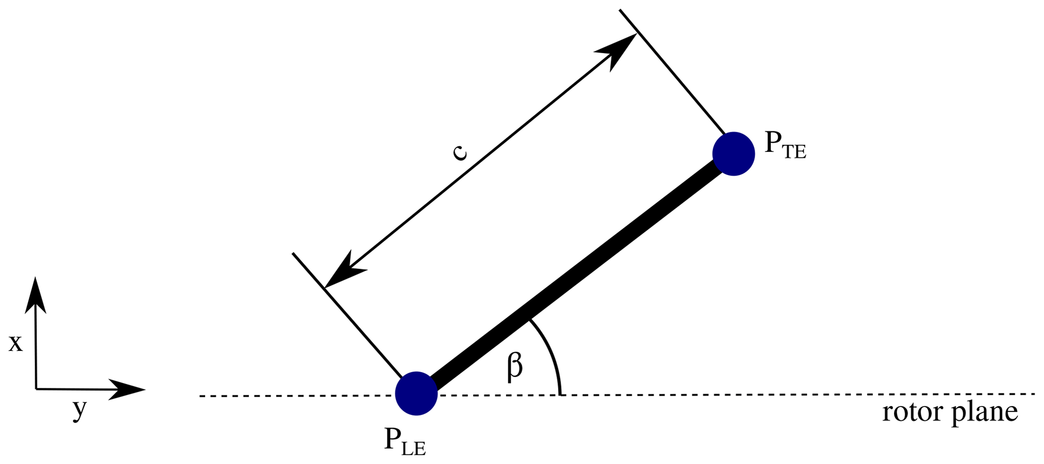
Figure 12 Determination of the pitch+torsion angle β out of DIC measurements. c: chord length of the rotor blade; x: OoP position; y: IP position.

Depending on the value of c, the resolution of the OoP position may need to be very accurate to determine the torsion angle. If c has a value of 700 mm, and β should be determined with a resolution of 0.1^∘, then dx needs to be resolved with an accuracy of 1.2 mm.

5 Results

This section contains measurement results of one DIC measurement time series and related simulations. The DIC measurement duration was 5 min, and the simulations were conducted for a 10 min time series based on the statistics of the wind conditions during the corresponding time slot. For the simulations, the aeroelastic solver BHawC (Siemens Gamesa in-house aeroelastic solver; Rubak and Petersen, 2005; Skjoldan, 2011) is used. BHawC has been used for almost 15 years for the simulation of loads of both onshore and offshore wind turbines. The structural model of the solver is based on the non-linear Timoshenko finite-element beam model based on a co-rotational formulation (Couturier and Skjoldan, 2018). The structural model is coupled with a standard blade element momentum (BEM) code including a Beddoes–Leishman-based dynamic stall model, a second-order dynamic inflow model, a standard Prandtl tip-loss correction, and a Glauert-type yaw misalignment correction as well as an empirical correction for heavily loaded rotors.

The aeroelastic simulations are carried out in a so-called one-to-one fashion (see Enevoldsen, 2014). The structural model is matched exactly to the particular turbine in geometry and structural description. In addition to this, the system dynamics are represented in high resolution as the atmospheric inflow conditions are recreated numerically according to the statistics of the wind corresponding to that exact time series. Several turbulence boxes were generated for these conditions, all of them with the same statistics, with the aim of reducing the uncertainty. The wind field is modelled as accurately as possible with the available instrumentation and statistics collected, but a full wind field recreation based on time series measurements is not available. Usually, a minimum of 6 and a maximum of 20 simulations with the same statistical wind conditions but under variation in turbulence seeds are conducted for a time series. In this case, nine simulations were conducted to become independent of the influence of turbulent seeds.

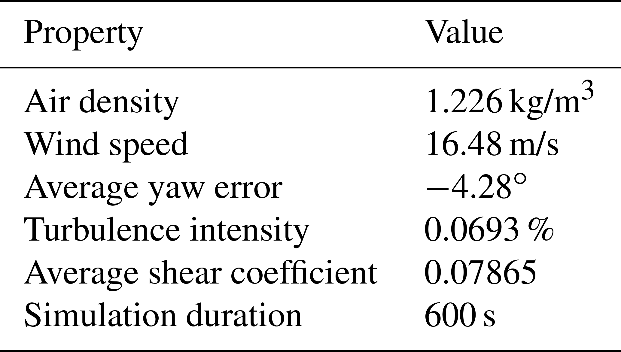
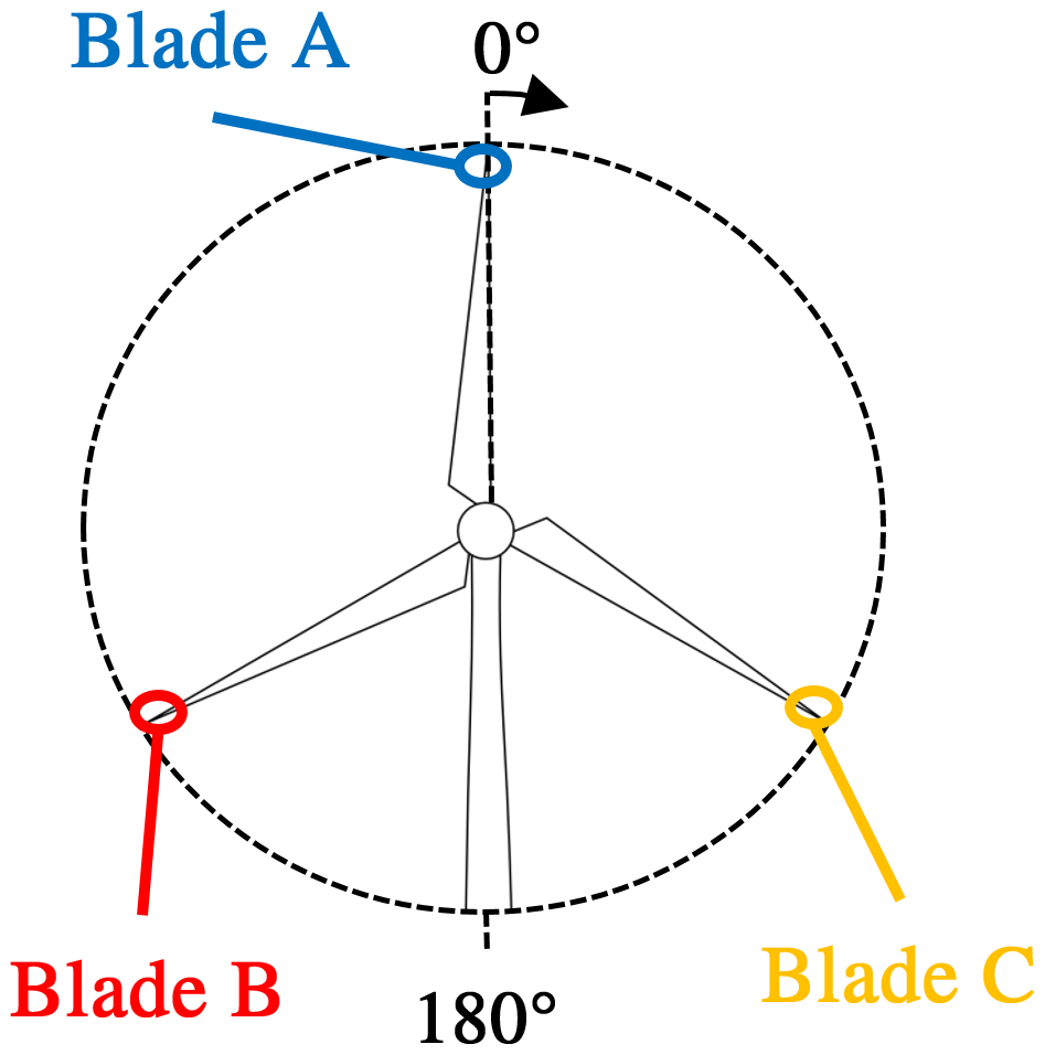
The statistics of the measured wind conditions during the time period are shown in Table 1. These conditions were measured by the ground-based lidar upwind of the turbine (see Sect. 2). The azimuth angle in the following diagrams is defined according to Fig. 13. From the DIC measurements, a point was chosen which is placed on a radial position of 56.5 m, and the numerical model was set up to have an output point at the same radial position. Therefore, all following results for measurements and simulations were extracted at a radial distance of approximately 56.5 m distance to the blade root.

Table 1 Statistics of measured wind conditions as input for simulations.

Figure 13 Definition of azimuth angle.

5.1 Rotor blade deformation

Figures 14 to 17 show the output of processed DIC measurements on all blades. In the OoP time series the influence of a continuous change in pitch angle can be clearly seen. At the beginning of Fig. 15, an asymmetric flap-wise vibrational behaviour can be seen on all rotor blades for a few seconds. A direct comparison of OoP and IP deformation shows that the amplitude of IP deformation is higher compared to OoP.

Figure 14 OoP DIC signal of all blades.

Figure 15 OoP DIC signal of all blades – close-up.

Figure 16 IP DIC signal of all blades.

Figure 17 IP DIC signal of all blades – close-up.

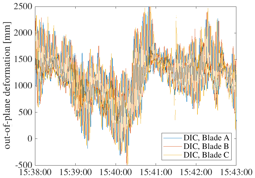
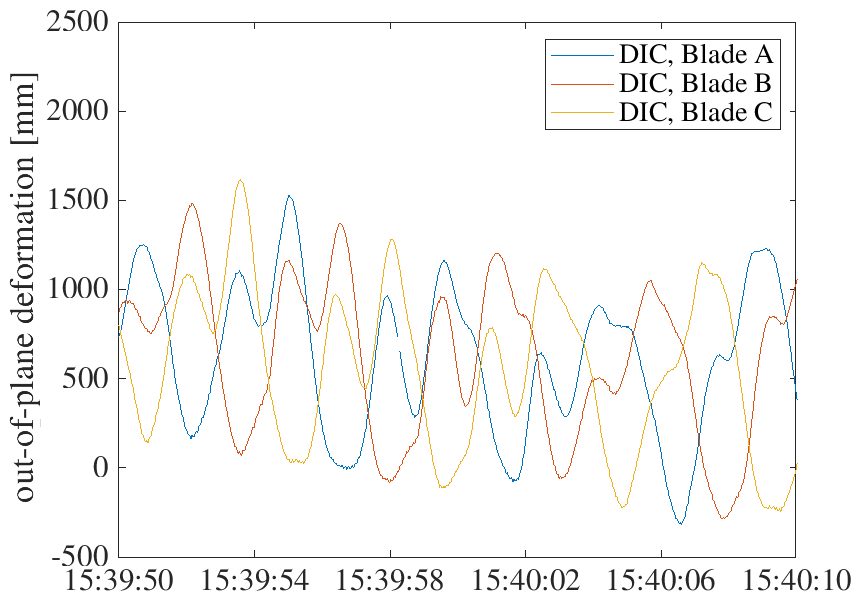
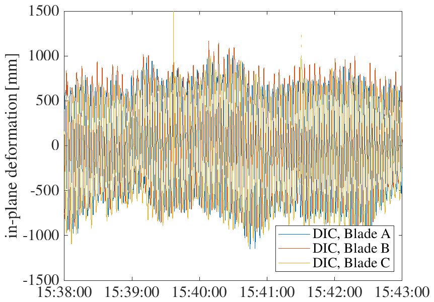
Figure 18 shows a qualitative comparison of the flap-wise bending moment in the blade root and the deformation at the blade tip in the OoP direction.

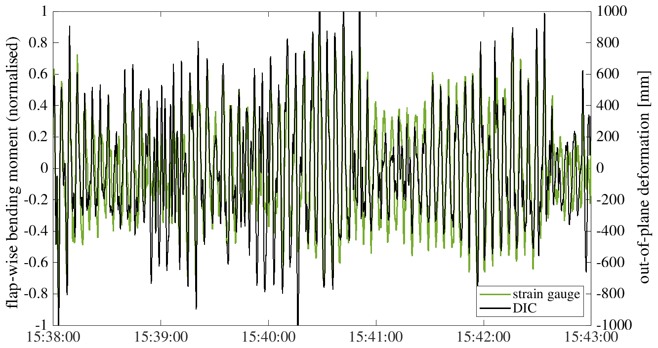
Figure 18 Qualitative comparison of measured flap-wise bending moment and OoP deformation of blade B.

Both variables have been reduced by their moving average for an improved comparability. It can be seen that the qualitative behaviour of both variables is nearly identical, which confirms that the OoP deformation of rotor blades, measured with DIC, corresponds to the flap-wise loads prevailing in reality. The same behaviour can be observed for IP deformation in comparison with the edgewise bending moment.

Comparison with aeroelastic simulations

In Figs. 19 and 20, a cut-out of OoP and IP deformation of blade B measured with DIC is shown in direct comparison with simulation results over time. The simulation results are presented as the mean and standard deviation of all nine simulations that were conducted. At first sight, the OoP DIC signal shows differences in the position of the minimum and maximum deformation, while the IP DIC signal is in very good agreement with the simulations.

For a better comparison over the whole time series, the deformation is plotted against the azimuth angle. Figures 21 and 22 show the mean results for OoP and IP deformation against azimuth angle. The simulation results are again summarised to obtain mean and standard deviation values. The values are divided into 1^∘ bins of azimuth angle, and the values for the corresponding mean value and standard deviation are obtained.

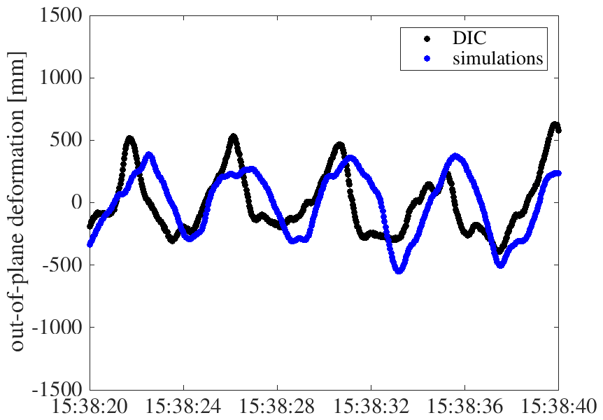
Figure 19 Comparison of OoP deformation measurement and simulations of blade B – short time series.

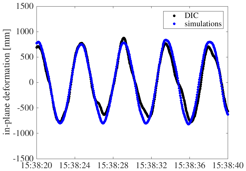
Figure 20 Comparison of IP deformation measurement and simulations of blade B – short time series.

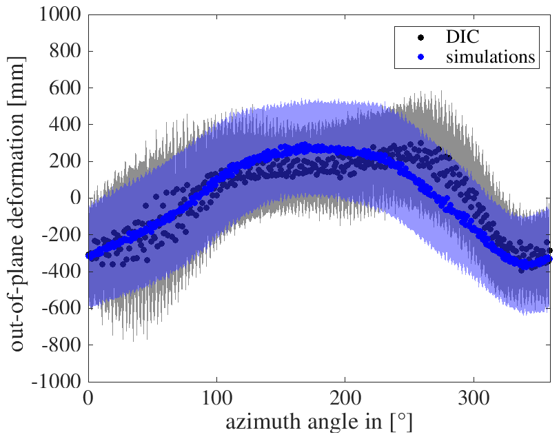
Figure 21 Comparison of OoP deformation of DIC and simulations of blade B – mean values with standard deviation.

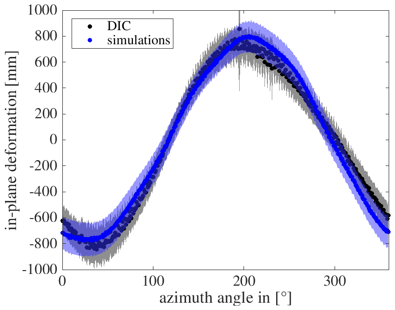
Figure 22 Comparison of IP deformation of DIC and simulations of blade B – mean values with standard deviation.

In general, the OoP deformation measured with DIC is in good agreement with the simulations. Overall, the simulations and measurements always overlap within the band of standard deviation, and the maximum and minimum amplitude have a similar value. However, the maximum OoP deformation for simulations of blade B appears at approximately 180^∘, while for DIC it is shifted and appears at around 250^∘. One reason for this could be an influence of the actual prevailing weather conditions. The simulations are based on statistics of the wind measurements of 10 min, while the measurements are a result of the real wind conditions, which can be different in this case.

The IP deformation of DIC is in very good agreement with the simulations, which is shown in Fig. 22. The location of minimum and maximum IP deformation is nearly the same, and so is the amplitude and the related standard deviation.

5.2 Rotor blade torsion

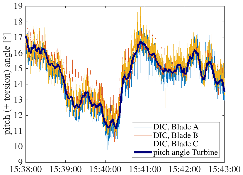
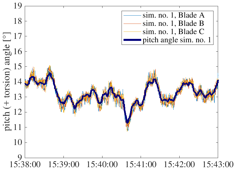
A result for the combination of rotor blade pitch and torsion angle measured with DIC is shown in Fig. 23. The DIC signal clearly follows the pitch signal of the turbine for all three blades. In comparison with results from simulation no. 1, as shown in Fig. 24, the amplitude of measured torsion is higher. In reality, the pitch signal has a higher range (from 17 to 11^∘) compared to simulation no. 1 (from 14 to 11^∘), but this cannot explain the difference between measured and simulated torsion.

Figure 23 Measured wind turbine pitch angle and DIC pitch + torsion angle.

Figure 24 Simulated pitch+torsion angle of simulation no. 1 of all blades.

Figure 25 Comparison of torsion angle of blade A of DIC and simulations – short time series.

Figure 26 Coupling of rotor blade torsion and OoP deformation.

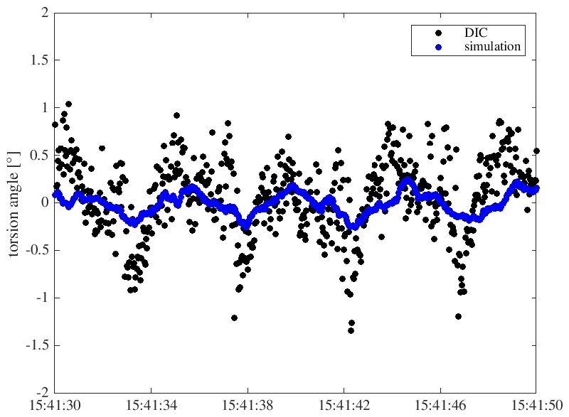
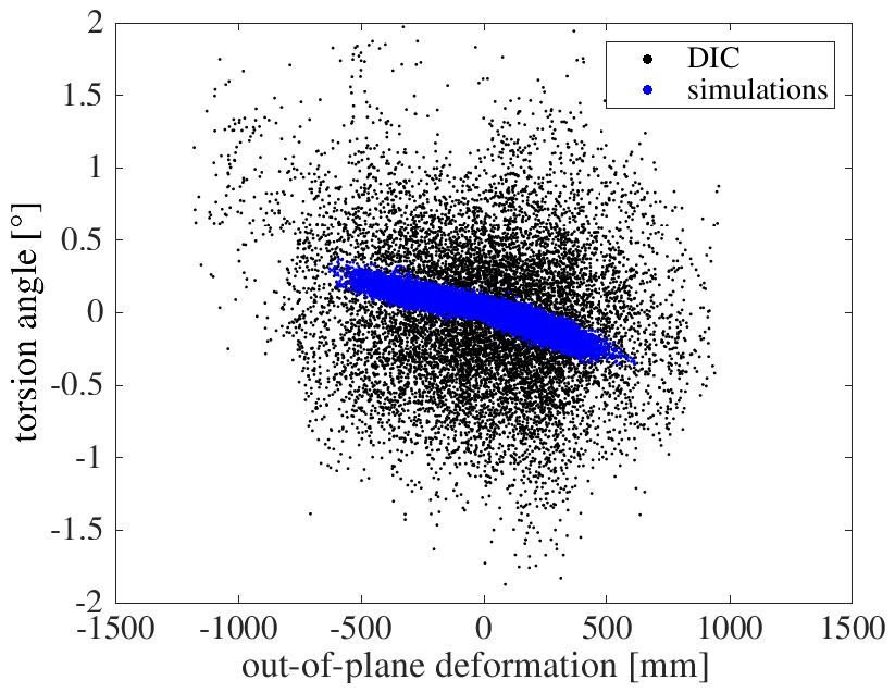
A direct comparison between measured and simulated torsion is shown in Fig. 25. The moving average has been removed from all data sets and shows clearly that the torsion measured with DIC is higher compared to simulations but generally shows the same trend. This becomes even clearer when the torsion is plotted against deformation, as shown in Fig. 26. The trend of the coupling between rotor blade torsion and OoP deformation can be reproduced from the DIC measurements but with a significantly higher amplitude.

The reason for this difference could lie either in an inaccuracy of the simulation or of the DIC measurement. However, if the torsion would have an amplitude as high as that measured with DIC, the actual measured loads would be expected to give significantly different values, too. As this is not the case, the dynamic amplitude of torsion measured with DIC is physically not plausible in this case. The reason for this is not clearly identified by now and will be further investigated. As it is known from past measurement campaigns, the spatial resolution and thus the accuracy of DIC can be improved by increasing the number of speckles on the blades, which will be taken into account for future measurement campaigns.

5.3 PSD

Lastly, deformations measured with DIC are compared to simulations and bending moments in the frequency spectrum obtained with Welch's method. Figure 27 shows the frequency spectrum of the flap-wise bending moment and the OoP deformation. The signal of strain gauges in the blade root from measurement and simulations is overall in good agreement. The measurement shows clear peaks at 1P and its multiples, whereas the simulations show a number of smaller peaks in the 2P range. For the OoP deformation, the PSD of the DIC signal is in good agreement with the simulations. The main peaks occur at 1P and its multiples. Right behind the 2P frequency, a small peak can be observed which belongs to the frequency of the first flap-wise mode.

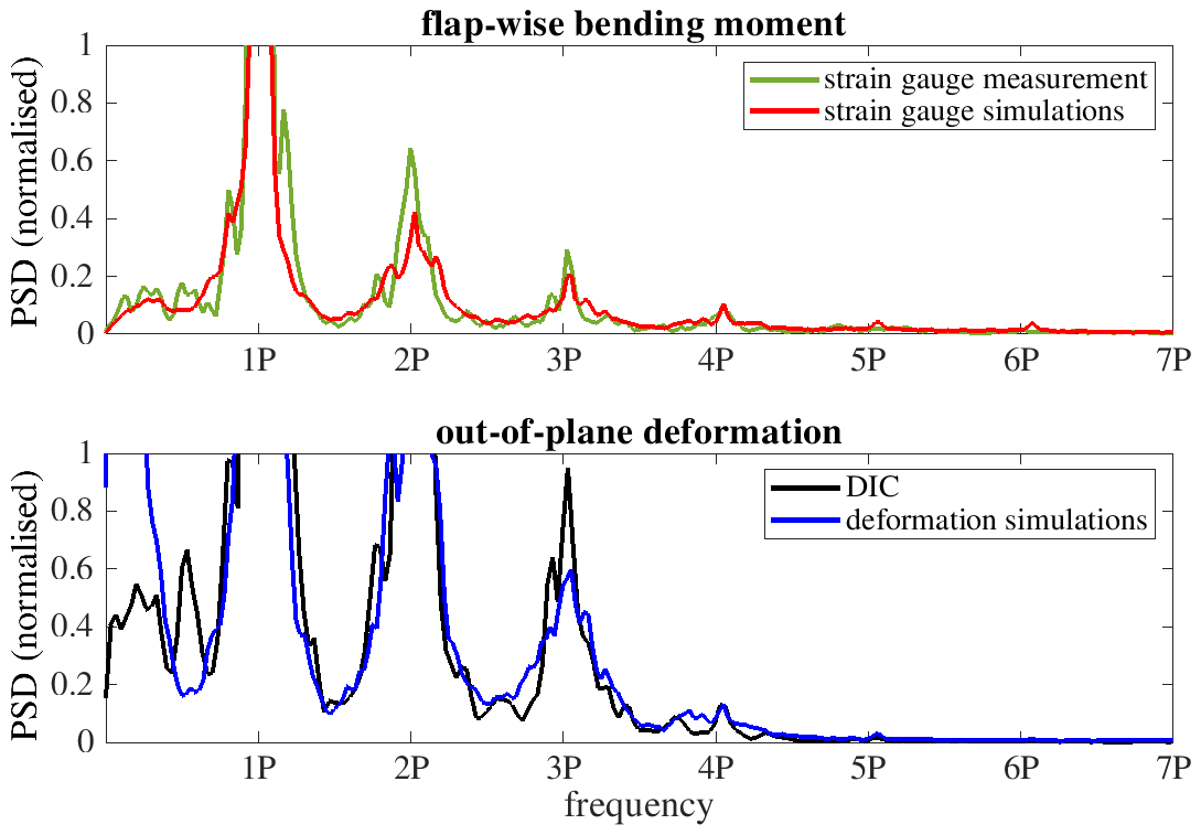
Figure 27 Comparison of PSD extracted with Welch's method for flap-wise and OoP signals of blade B.

The PSD of edgewise bending moment and IP deformation is shown in Fig. 28. The signal of strain gauges in the blade root from measurement and simulations is in good agreement. This proves that the simulated loads are close to the real loads in this time series. The first edgewise mode between 3P and 4P can be clearly identified out of both signals. The same peak can be observed in the PSD curves of the IP deformation measurement and simulations. Furthermore, the IP deformation measurement shows a peak right behind the 2P frequency, which belongs to the first flap-wise mode. A small peak at the frequency of the second flap-wise mode can only be seen in the PSD of the simulated flap-wise bending and IP deformation. A reason why this is not seen in the DIC signal could be that the radial measurement position is not exactly the same in simulation and measurement and that the DIC measurement point is closer to the node of the second flap-wise mode so that the amplitude is too small to be clearly observed.

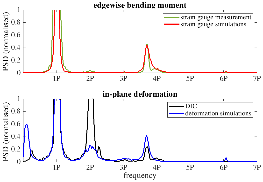
Figure 28 Comparison of PSD extracted with Welch's method for edgewise and IP signals of blade B.

6 Conclusions

This paper shortly summarises the functionality of DIC and the application of this innovative measurement technique to full-scale wind turbines. Furthermore, typical measurement results are shown, and a comparison with measured root bending moments and simulations is evaluated.

The results show that rotor blade deformations measured with DIC qualitatively show the same trend when compared to strain gauges in the blade root for both OoP and IP. A direct comparison of measured and simulated deformations shows that both are in very good agreement. Small deviations can be seen, especially for OoP deflections. Those deviations can occur from the statistical character of the simulations, which are hard to meet with a 5 min measurement. The simulations are based on the mean wind conditions of the same time slot, which can cause a difference between simulated loads and reality. A direct comparison of a short time series of deformation measurements with statistical simulations remains a challenge. But still the results of this paper prove that DIC is a suitable method for the validation of rotor blade deformation at full scale.

The measurement of rotor blade pitch and torsion angle with DIC in this set-up clearly follows the actual pitch angle of the turbine, which validates the method on average. However, the amplitude of the dynamic torsion is higher compared to simulations. This amplitude is not physically plausible as the expected loads of the turbine would then be different, too. The reason for this is not clear yet and will be further investigated. One approach could be to improve the experimental set-up as the present one can be considered to be minimalistic in that there were only 50 speckles applied on every blade. If the size of the speckles is reduced, the number of speckles on the blades can be increased, which would come along with an improved spatial resolution of the rotor. This will be taken into account for future DIC measurements.

In summary, DIC can be considered a suitable method to measure rotor blade deformation and torsion and to validate aeroelastic simulations. It can be easily applied on rotor blades, even if the blades are already installed on the turbine. In future work, the measurement accuracy for the rotor blade torsion will be improved by optimising the experimental set-up, in particular the speckle pattern on the blades, as well as the measurement equipment. Furthermore, a more detailed analysis based on a whole series of measurements will be conducted to perform a validation of aeroelastic codes with this short-term measurement technique. For this, SpinnerLidar data will be used to optimise the reconstruction of the wind field for simulations. DIC has great potential for the experimental validation of the simulations of rotor blade deformation and torsion of wind turbines.