the Creative Commons Attribution 4.0 License.
the Creative Commons Attribution 4.0 License.
 | 30 Oct 2020
Theory and verification of a new 3D RANS wake model
Philip Bradstock
Wolfgang Schlez
This paper details the background to the WakeBlaster model: a purpose-built, parabolic three-dimensional RANS solver, developed by ProPlanEn. WakeBlaster is a field model, rather than a single turbine model; it therefore eliminates the need for an empirical wake superposition model. It belongs to a class of very fast (a few core seconds, per flow case) mid-fidelity models, which are designed for industrial application in wind farm design, operation, and control.
The domain is a three-dimensional structured grid, a node spacing of a tenth of a rotor diameter, by default. WakeBlaster uses eddy viscosity turbulence closure, which is parameterized by the local shear, time-lagged turbulence development, and stability corrections for ambient shear and turbulence decay. The model prescribes a profile at the end of the near wake, and the spatial variation of ambient flow, by using output from an external flow model.
- Article
(765 KB) - Full-text XML
- BibTeX
- EndNote


In wind farms, wind turbines located downstream of other turbines will experience wake losses. Wind farm development and assessment processes require multiple iterations of configurations, as well as fast project turnaround.
A good understanding of how wake loss works can give a company the competitive edge, while an unexpected systematic performance loss can eliminate the expected profit from a project, or even from an entire project pipeline. Given the importance of wake losses, it may appear contradictory that many in the industry still use analytical single turbine wake models. Using single turbine wake models means that the wake from each turbine is propagated independently, wake expansion is not impacted by neighbouring wakes, and multiple wake deficits are superimposed using an empirical wake superposition model. Single wake models are based on an approach suggested 40 years ago, by Lissaman (1979) and Lissaman et al. (1982), who transferred the work of Abramovich (1963) on free jets to wind turbine wakes. Jensen (1983) presented what is still the most prominent model in this category. Other prominent models of this type include numerical solutions, by Ainslie (1988) and Ott (2011). More recent analytical models include that of Ishihara and Qian (2018).
The longevity of the single wake model approach also speaks for the quality and practical usefulness of these early models. However, in order to provide accuracy for the full range of wind farms (e.g. large wind farms, closely cross-spaced farms, low hub height wind farms, wind farms with stable conditions, or offshore wind farms), an increasing number of empirical corrections had to be made, and parameters added, informed by new experimental data from wind farms, scale experiments, or higher-fidelity models – see, for example, Liddell et al. (2005), Schlez et al. (2006), Schlez et al. (2009), and Beaucage et al. (2012). A range of analytical single wake models and superposition methods are reviewed by Porté-Agel et al. (2020).
The increased computational power and scalability available today allows higher-fidelity wake models to be used in the iterative process of wind farm design. These models widen the operational envelope, include more physics, and reduce model uncertainties in non-standard situations. The theory behind one such model is presented in this paper: a 3D RANS (Reynolds-averaged Navier–Stokes) wind farm wake model, WakeBlaster.
Related work
In order to gain a more detailed understanding of wake losses in a wind energy research context, two groups of 3D RANS codes have been developed. The models are referred to as “field models”, to distinguish them from the single turbine models by Crespo et al. (1999).
The first group of 3D RANS codes consists of parabolic solvers, using the thin shear layer approximation; see Ferziger and Perić (1999). Parabolic solvers assume a dominant flow direction, and information is transported only downstream. Crespo et al. (1988) developed UPMWAKE at UPM (Universidad Polytéchnica de Madrid), and later Crespo et al. (1994) developed an extension for wind farms, called UPMPARK. A number of further variants have been developed and reviewed by Vermeer et al. (2003). One branch was continued by TNO/ECN (Energy Research Center of the Netherlands), and it resulted in the WakeFarm presented by Schepers (2003) and FarmFlow model presented in Eecen et al. (2011). Renewed interest in mid-fidelity models has recently led to the independent development of several new models in this group, like those presented by Trabucchi et al. (2017) and Martínez-Tossas et al. (2020).
The second group of 3D RANS field models, the elliptic solvers, is more widespread. Elliptic solvers are generally more powerful, and they iterate equations numerically, in order to allow information to be transported in all directions; this makes them more expensive computationally (by several orders of magnitude). These models use a k–ϵ or k–ω turbulence closure, describing the generation and dissipation of turbulent kinetic energy. Models in this group are (in principle) also capable of solving upstream effects, such as the interaction of wakes in the induction zone, and the near wake of wind turbines. Some models are based on general-purpose flow solvers, whereas others are in-house developments – examples can be found in publications by Crespo et al. (1988), Prospathopoulos et al. (2010), Barthelmie et al. (2011), van der Laan et al. (2017), and Sørensen (1995).
The WakeBlaster model developed by ProPlanEn by Schlez et al. (2017b) belongs to the parabolic solver group. A parabolic solution offers a good balance between improved accuracy, additional detail, and computational costs. The target of the new model is to improve the accuracy of wind farm loss modelling. Two specific aims are to address the interaction between wakes, as well as the interaction between wakes and the atmospheric boundary layer for different levels of atmospheric stability. Special attention was paid to the validation of the model, using data from a wide range of wind farms and atmospheric conditions, which has been reported by the authors in Schlez et al. (2017a), Schlez et al. (2018), Schlez et al. (2019), Bradstock et al. (2018), and Braunheim et al. (2018) and independently evaluated and compared to engineering models in a blind test for offshore wind farms by Sanz et al. (2019).
The fundamental equations and assumptions for this solver are shown in the Sect. 2. Section 3 presents as example the verification of the model for an offshore wind farm and the results of verifying the computational performance. Section 4 discusses model limitations, followed by the conclusions in Sect. 5.
The WakeBlaster wind farm simulator is based on a Reynolds-averaged Navier–Stokes (RANS) set of equations, which is used to solve the propagation of wake dissipation through the farm domain, in Cartesian 3-dimensional coordinates. In order to account for the fluctuation term of the velocity vector, it uses eddy viscosity turbulence closure, where the eddy viscosity is calculated from the combined wake and ambient wind speed shear profiles.
2.1 RANS equations
The wake model uses RANS equations for momentum conservation and mass flow conservation to calculate the three components of wind velocity in the axial, lateral, and vertical directions. Cartesian 3-dimensional vectors are used for displacement x and wind speed relative to ambient u: , where the first element of the vectors (x) is the streamwise component, the second element (y) is horizontal and perpendicular to (x), and the third element (z) is vertical (starting from the ground up) and makes up a right-hand coordinate system.
The Reynolds-averaged momentum and mass conservation equation can be expressed in two dimensions, for either a free jet or a wake submerged in an incompressible fluid, as given by Abramovich (1963):
representing the momentum in the flow direction, where u′, v′, and w′ denote fluctuations from mean values, and ν the viscosity and ρ the density of the fluid. The corresponding continuity equation is
The momentum equations in transversal directions are not considered in the description of a free jet or wake present beyond the near wake of a wind turbine.
2.2 Simplifying assumptions
The following simplifying assumptions are applied by Abramovich for a stationary free wake, expanding into an infinite region:
- Viscosity
-
The effect of molecular viscosity is small compared to the turbulent viscosity.
- Pressure
-
Flow pressure gradients can be neglected in most cases .
- Stationary
-
The flow is stationary with respect to the mean velocities .
- Thin shear layer approximation
-
Fluctuations along the flow change much slower than in the transversal direction .
After substituting the continuity equation and applying the simplifying assumptions, Abramovich (1963) obtains
and expanded to three dimensions:
Using the Boussinesq eddy viscosity assumption, the stress components and are expressed as
where ϵ denotes the isotropic eddy viscosity. The streamwise variation in transversal velocities is small compared to the transversal variation of streamwise velocity . The spatial variation in eddy viscosity can be neglected in first approximation and is therefore approximated as a constant. The governing momentum conservation equation can now be written as
2.3 Numerical solution
The ambient wind field is determined by an external flow model, and it determines the inflow conditions and spatial variations over a site. The turbine is represented by its hub height, diameter, and other readily available and measured characteristics.
2.3.1 Model domain
The waked wind field is set up by creating a two-dimensional flow plane, which forms a cross section along the y and z axes of the velocity vector . The flow plane is propagated downstream along the x coordinate, and when it passes a turbine, a wake is injected into the flow plane.
The grid spacing is set by default to 0.1 D (rotor diameter). In the vertical direction, the grid starts at the ground z=0 and reaches up to a default height of 3 D or 31 grid layers. In the horizontal direction, the grid is expanded, as required, to enclose each wake injected into the flow plane with an additional 4 D to the side to allow for wake expansion.
2.3.2 Wind turbine momentum extraction
Axial-momentum theory prescribes pressure building up in the induction zone upstream of any wind turbine or wind farm and pressure recovery in the near wake downstream of the rotor. The momentum that each of the turbines extracts in the process is the wind-speed-dependent thrust coefficient, as a function of the idealized incident wind speed, Uinc, at each turbine location, without the presence of the turbine.
In the model, the momentum deficit is injected at the end of the near wake (which is assumed to be at 2 D downstream of the rotor) of each turbine, and it is distributed over an expanded rotor area, using the blunt bell-shaped wind speed deficit profile from Lissaman et al. (1982). The centre-line wind deficit relative to incident wind speed Dm, experimentally determined by Ainslie (1988) at a downstream distance of 2 D, is used as a function of inflow turbulence Iinc and thrust coefficient ct.
The radial width of the profile is then derived by ensuring momentum conservation with regard to the thrust coefficient of the turbine.
2.3.3 Flow plane propagation
The flow plane is propagated according to Eq. (6) using the alternating direction implicit (ADI) method described by Peaceman and Rachford (1955) and von Rosenberg (1983), where it is alternately solved in the x–y and x–z planes, incrementing the x (downstream) coordinate by half a propagation step between each solving plane, so that both planes are solved once per step. By solving for each row or column in the flow plane, and by employing the central difference method, the problem can be set up numerically in a tridiagonal matrix equation, which can then be solved efficiently for the axial velocity, u, by the Thomas algorithm Thomas (1949), described for example in Burden and Faires (2001). In 3-dimensional Cartesian coordinates the tridiagonal equation must be solved for every row or column of the flow plane, depending on which direction a solution is obtained. Dirichlet boundary conditions are used by enforcing u=1 in the extremities of the flow plane.
At each half-step of the solving process, the horizontal and vertical velocities, v and w respectively, are calculated for all points in the flow plane according to Eq. (2). For any given step there are two unknowns in this equation, v and w, and therefore it cannot be solved analytically in a single step. Instead, the unknowns are calculated numerically, by calculating each individually, and iterating until their values converge. By rearranging equation 2, v and w can be expressed individually for a parabolic flow:
In practice, due to the assumption of incompressibility, this formulation will lead to a local velocity shear, resulting in non-zero lateral and vertical velocities that are infinitely far from the source of shear. In reality this would not be the case, due to the compressibility of air. Therefore, in order to account for the effect of compressibility, a spatial damping term is introduced so that v and w tend to zero at , y=∞, and z=∞:
where γ is a user-configurable positive constant that determines the strength of lateral and vertical velocity damping. As these integrals are indefinite, boundary conditions must be assigned. In the vertical direction, it is given that vertical velocity at ground level is zero, as mass flow cannot pass into or out of the ground. Therefore, the condition is applied, leading to
In the lateral direction, the physical boundary conditions are that , because the wind farm wakes cannot induce lateral velocity far from the farm. However, for numerical purposes, the size of the flow plane is constrained, and it cannot be guaranteed that the velocity will reach zero on both sides of the flow plane. Therefore, the lateral velocity is integrated in each direction, starting from zero, and the mean of the two is taken. This is expressed as
where ymin and ymax are the lateral location of the edge of the flow plane.
2.4 Eddy viscosity calculation
The key term controlling the rate of wake dissipation is eddy viscosity. Eddy viscosity has dimensions of length squared over time, and it can be represented by multiplying a length scale of the shear layer by a velocity scale of the flow field.
WakeBlaster calculates eddy viscosity from the shear profile of axial velocity in the y–z plane. In order to do this, it creates a combined flow plane of the ambient wind speed, Uamb, multiplied by the solved wake flow plane, u, which is relative to ambient wind speed. In neutral atmospheric conditions, the ambient wind speed is calculated as a logarithmic function of height above ground:
where u* is the friction velocity, taken to be 2.5 times the value of standard deviation of the axial wind velocity, κ is the von Kármán constant (value = 0.4), and z0 is the roughness length. The unknown parameters are determined from inputs to the simulation, such as wind speed and turbulence intensity at a particular height (usually the hub height of one of the turbines). The eddy viscosity is then calculated for every point in the flow plane, using the following process:
-
Create a combined flow plane by multiplying the ambient surface layer wind speed profile by the waked flow plane velocity u.
-
For each point, identify the local minimum and maximum velocity. For a point located at (y,z), local is determined as the range and , in the lateral and vertical directions respectively, where η is a configurable constant which meets the criterion .
-
In each of the two directions, the component of eddy viscosity is calculated as ϵi=ΔuiΛi, where Δui is the difference between minimum and maximum velocity and Λi is the distance between the maximum and minimum points. This process is shown in Fig. 1.
-
The overall eddy viscosity is the calculated as , where k is a positive calibration constant, which although configurable is considered to be independent of wind farm size and layout.

Figure 1Calculation of the vertical component of eddy viscosity by finding the points of minimum and maximum velocity within a given height range.
For a logarithmic wind speed profile in the vertical direction with no lateral variation, this method leads to an eddy viscosity that is proportional to the height above ground.
2.4.1 Eddy viscosity lag
The eddy viscosity, as so far described in Sect. 2.4, is solely based on the wind shear profile. However, no newly created shear profile instantly generates turbulence and therefore eddy viscosity – in reality, there is a lag between the change in a shear profile and its effect upon eddy viscosity and wake dissipation. In WakeBlaster this lag is formulated in terms of downstream distance, and it has two distinct models.
The “fixed” model obeys a first-order lag equation:
where ϵ is the lagged eddy viscosity, Λ is the length scale defined in the previous section, and ℓ a positive constant defining the lag length relative to the length scale and considered to be independent of wind farm size or layout.
The “turbulence-dependent” model gives a larger lag distance when the eddy viscosity and turbulence are low, and it obeys the following equation:
where ϕ is a positive parameter that determines the strength of turbulence on the lag length, and λmax is also a positive parameter that corresponds to the lag length when turbulence is zero. Both parameters are calibrated against extensive wind farm observational data and are considered to be independent of wind farm size and layout.
2.4.2 Atmospheric stability
When simulating atmospheric conditions that are not neutral, the calculation of eddy viscosity is modified. This modification uses the Monin–Obukhov length, L, and the concept of non-dimensional wind shear, ϕm, which is defined by Businger (1971), as
Furthermore, according to Businger (1966), the non-dimensional wind shear is empirically approximated as what tends to be known as the Businger–Dyer relationship:
where . The ambient wind speed shear profile is then modified by introducing ψm:
where
where . Furthermore, the vertical component of the eddy viscosity, ϵz, is also modified by the non-dimensional wind shear:
The horizontal component of eddy viscosity, ϵy, is left unmodified.
2.5 Wind turbine power calculation
WakeBlaster calculates the power output using power curve input from the user. In order to calculate accurate power, corresponding to the variant wind speed across the rotor, a rotor-equivalent wind speed (Urot) is calculated. This is done by first calculating the combined ambient and wake axial velocity (U=Uambu at the rotor plane) and then integrating across the rotor disk area:
where n is an integer. A popular approach is to use n=3 as suggested in IEC61400-12-1 (2017), based on the principle that the power available in the wind is proportional to the cube of the wind speed. However, WakeBlaster uses a value of n=1 by default as turbines will not be able to realize the full potential of a sheared inflow over the rotor. As this method is performed on the combined ambient and wake axial velocity, the effects of wind shear on power production are implicitly included whenever the severity of the wind shear depends on the turbulence and atmospheric stability of the flow case.
A general directional variability of the wind within each flow case is included in a standard power curve. A rotor yaw angle can be set per turbine, to consider in the power calculation a known average directional misalignment with the rotor plane. A model to modify the power curve for site-specific directional variability over the rotor, for example changes with height or for specific meteorological conditions, is not included in the model.
WakeBlaster uses IEC methods in IEC61400-12-1 (2017) to adjust the power curve for air density and turbulence intensity. The rotor-equivalent turbulence intensity is also calculated using the integral method above but instead using a value of n=2.
In this section, the grid dependence and sensitivity is analysed, and an estimate of the numerical uncertainty is thereby provided. Computational performance for large wind farms is verified, and offshore wind farm model predictions are inspected graphically for plausibility.
3.1 Grid dependence and sensitivity
The model uses a structured grid, in terrain-following coordinates. The grid resolution is scaled with a length scale characterizing the specific flow – the rotor diameter. The grid is equally spaced in all directions, and no stretching, compression, or nesting is applied to any part of the domain. The minimalist design is computationally efficient, and it avoids potential numerical errors – at grid interfaces which do not match, for example.
The solver is designed for a single purpose: to model the impact of wind turbines on the underlying flow and the consequential wind farm wake losses. A wind turbine's wake scales with its rotor diameter and its height above ground. In order to match the dominant scale in the flow for each wind farm, the grid resolution is fixed at 0.1 D; it thus scales with the rotor diameter.
Analysis of the sensitivity of model results to changes in grid resolution verifies that the results are not sensitive to grid resolution over the expected range of application. Challenges could arise – for example, when using an average resolution in wind farms with mixed turbine diameters and turbines mounted at low hub heights. In an annual energy calculation, the overall wake loss is composed of several thousand individual flow cases. Wake loss model errors are commonly estimated to be in the range of 10 %–20 %, relative to the average annual wake loss. Numerical errors should be 1 order of magnitude lower. Ignoring error compensation between flow cases, an error of 1 %–2 % (relative to the wind speed difference for an individual flow case) is acceptable.
The grid dependency study was carried out for the following scenario: a single turbine, with ambient wind speed perpendicular to the rotor plane. Ambient conditions were a wind speed of 8 m s−1, neutral atmospheric stability, and a turbulence intensity of 10 %. The wind turbine type (V100-1.8) is described by its geometry and thrust coefficient, which is ct=0.8 for the scenario. The key target value investigated is the wind speed relative to ambient wind speed, at hub height and at several distances downstream.
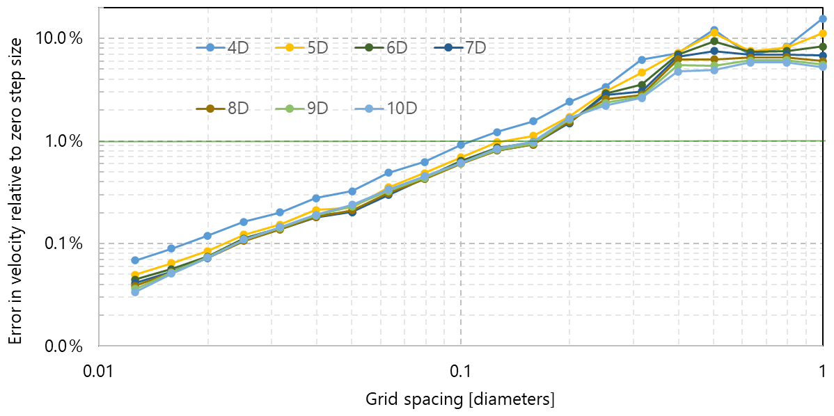
Figure 2Numerical error due to the grid spacing, based on the difference in wind speed from the hypothetical zero grid spacing value calculated by Richardson extrapolation. The scenario assessed has an ambient wind speed of 8 m s−1 and ct=0.8, neutral atmospheric stability and 10 % turbulence. The acceptable numerical error is shown as 1 %.
The sensitivity was tested in a flow case with a strong wake, and the results are presented in Fig. 2. The error in wind speed is presented relative to a hypothetical error value, which is calculated using a Richardson extrapolation for an infinitesimal grid spacing, as suggested by Roy (2003) for mixed-order numerical schemes.
The numerical error, due to grid spacing for an operational range of up to just above 0.1 D, is below 1 %. At a coarser resolution the model can no longer resolve the structure of the flow sufficiently. The current choice of grid resolution (0.1 D) represents a reasonable compromise between computational efficiency and model accuracy.
The grid resolution in the model scales automatically with the rotor diameter. Neither the grid nor the resolution is a variable which should (under normal circumstances) be adjusted by any user.
3.2 Computational performance
WakeBlaster is a medium-fidelity tool, which is typically capable of running each flow case in a few seconds, on the single core of a modern processor. With the default settings (a flow plane resolution of 0.1 D and a domain height of 3 D), the time (in seconds) to run a single flow case (Tfc) is (on an Intel i5 8th-generation processor) approximately
where A is the area of the wind farm and D is the rotor diameter. The Tfc is proportional to the area of the wind farm and (at equal turbine density) to the number of wind turbines on the wind farm. However, the exact time will depend on the wind farm's layout, the wind direction, and the architecture of the processor. The Tfc is also proportional to the cube of the flow plane resolution, although results do not show any significant improvement in accuracy when the resolution is increased.
For example, a typical flow case for Horns Rev – a wind farm with 80 turbines arranged in a grid, with inter-turbine spacing of 7 D – runs in about 5 s. Unless hysteresis effects are included in a time series simulation, each required flow case remains independent of the others, allowing many flow cases to be run in parallel. As WakeBlaster is hosted on the cloud, this allows a high level of parallelization across tens or hundreds of processors, meaning that an energy assessment consisting of (for example) 2000 flow cases can be completed in a matter of minutes, even for large wind farms.
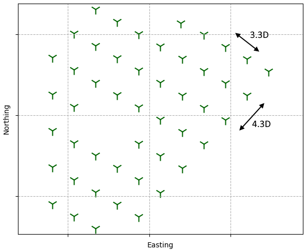
Figure 3Layout of the Lillgrund wind farm. The turbine rotor diameter is 93 m with a hub height of 68 m. The turbine spacing is approximately 4.3 D, along the south-west to north-east rows, and 3.3 D along the south-east to north-west rows.
3.3 Visual verification
Using a three-dimensional wake model, it is possible to create plots of the three-dimensional waked flow field for the complete wind farm, for a particular flow case. This article presents a visualization of a single flow case from the Lillgrund wind farm, located in the Øresund Strait, between Sweden and Denmark. The Lillgrund wind farm presents a good case study, because the small spacing between turbines (3.3 and 4.3 D, along the two principal rows) leads to large wake effects. The layout is shown in Fig. 3. The turbines have a rotor diameter of 93 m and a hub height of 68 m above mean sea level.
Three cross-sectional slices in the x–y, x–z, and y–z planes, for a flow case of 8 m s−1 wind speed, 270∘ wind direction, 6 % turbulence intensity, and neutral atmospheric conditions, are presented in Fig. 4.
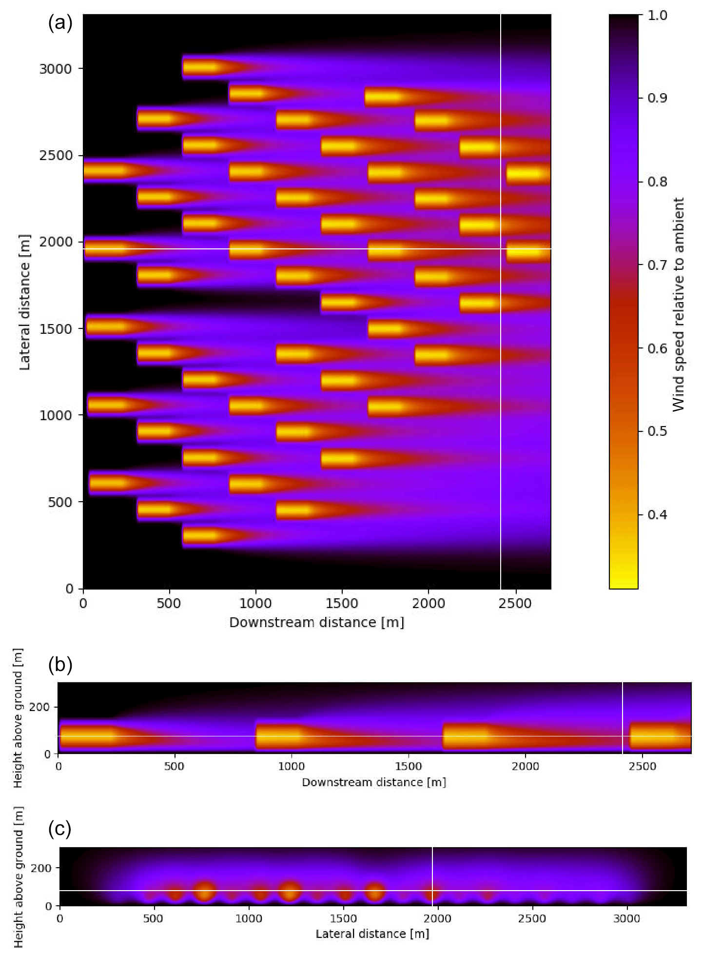
Figure 4Plots of the axial velocity on the wind farm relative to ambient wind speed for a flow case of 8 m s−1 with the wind from the west. From top to bottom, (a) x–y (bird's-eye) slice at hub height, (b) x–z (side-on), and (c) y–z (front-on). The white lines show the corresponding planes of the other plots. The x–y plot is taken at the turbine hub height above sea level – 68 m.
These simulations indicate that there is significant interaction between wakes originating from individual turbines, and this supports the assumption that the wakes cannot be modelled independently. The wake interaction leads to a complex wake shape downstream of the wind farm. The low hub height of the wind turbines (68 m), relative to their rotor diameter (93 m), results in significant ground–wake interaction effects. As ambient mixing from below is limited, single turbine wakes become asymmetrical in shape, and the point of greatest deficit drifts downwards to below hub height.
The code is a mid-fidelity code designed to be fast and capable of simulating projects with several thousand turbines, working with limited amount of readily available input data, and be used in an iterative design process. This limits the level of detail that can be included in the submodels.
-
No direct interaction between the turbines and no description of the axial pressure gradient are included in the model. The induction zones directly upstream and downstream (near wake) of turbines can overlap and interact. This may lead to changes in turbine performance and turbine characteristics, and no attempt has been made to quantify such effects.
-
A basic representation of the ambient flow is used as input to the model. The wake is modelled as a perturbation of the underlying flow. No attempt has been made to model a two-way interaction with the atmospheric boundary layer.
-
The model uses the directional speed-ups predicted by a suitable flow model (for example in a RSF/WRG format) to account for spatial variation of the wind resource, for example due to orography, or roughness. Further complex terrain effects, like flow separation, are not considered.
-
The ambient wind direction is assumed to be constant throughout the wind farm. Therefore in curved flows (due to terrain or due to meteorological factors), downstream wake locations may not be accurate.
The WakeBlaster model undergoes continuous, data-driven improvement, and refined models will be added successively.
This is the first publication to present the theoretical background of WakeBlaster in some detail. WakeBlaster is a recently developed 3D RANS solver that is specialized to simulate the waked flow field on wind farms. The characteristics of this model show the desired performance balance between speed and level of detail.
WakeBlaster calculations are provided as a cloud service and designed for integration in other software packages. WakeBlaster is available from ProPlanEn directly (https://www.proplanen.info/wakeblaster, ProPlanEn, 2020) and through third-party implementations. A WakeBlaster interface was integrated into EMD's WindPro software and UL's Openwind software in 2020.
PB carried out the following: formal analysis, investigation, methodology, software development, data curation, verification, visualization, and writing. WS carried out the following: conceptualization, funding acquisition, project administration, resources, investigation, supervision, methodology, and writing.
WakeBlaster is a commercial product of ProPlanEn Ltd. Wolfgang Schlez is the founder and sole shareholder of ProPlanEn Ltd. Philip Bradstock was employed by ProPlanEn Ltd at the time of carrying out the model development. He is a director of Bitbloom Ltd, providing services to ProPlanEn Ltd.
This article is part of the special issue “Wind Energy Science Conference 2019”. It is a result of the Wind Energy Science Conference 2019, Cork, Ireland, 17–20 June 2019.
A number of companies contributed operational wind farm data to this research, and their support is greatly appreciated. ProPlanEn GmbH processed the Lillgrund test case, as part of IEA task-31: WakeBench. The contributions of Staffan Lindahl and Sascha Schmidt (verification and visualization), Michael Tinning (software development), and Vassilis Kostopoulos (verification, investigation, and methodology) are acknowledged.
This research was co-funded by the UK's innovation agency, Innovate UK (grant no. 132381).
This paper was edited by Jens Nørkær Sørensen and reviewed by Paul van der Laan and one anonymous referee.
Abramovich, G. N.: The Theory Of Turbulent Jets, M.I.T Press, Cambridge, Massachusetts, USA, 1963. a, b, c
Ainslie, J.: Calculating the Flowfield in the Wake of Wind Turbines, Journal of Wind Energy and Industrial Aerodynamics, 27, 213–224, 1988. a, b
Barthelmie, R., Frandsen, S., Rathmann, O., Hansen, K., Politis, E., Prospathopoulos, J., Schepers, J., Rados, K., Cabezon, D., Schlez, W., Neubert, A., and Heath, M.: Flow and Wakes in Large Wind Farms: Final Report for UPWIND WP8, Tech. Rep. Risø-R-1765 (EN), Risø, 2011. a
Beaucage, P., Brower, M., Robinson, N., and Alonge, C.: Overview of Six Commercial and Research Wake Models for Large Offshore Wind Farms, in: European Wind Energy Association Conference 2012, 2012. a
Bradstock, P., Schlez, W., Lindahl, S., and Schmidt, S.: Reduction of Wake Modelling Uncertainty Using a 3D RANS Model, in: WindEurope Global Wind Summit, Hamburg, Germany, available at: https://windeurope.org/summit2018/conference/proceedings/ (last access: 23 October 2020), 2018. a
Braunheim, F., Schlez, W., and Jothiprakasam, V.: Wind farm simulation and validation of analytical and CFD based Wake Models, in: WindEurope Global Wind Summit, Hamburg, Germany, 2018. a
Burden, R. L. and Faires, J. D.: Numerical Analysis. 2001, Brooks/Cole, USA, 2001. a
Businger, J. A.: Transfer of Heat and Momentum in the Atmospheric Boundary Layer, in: Proc. Arctic Heat Budget and Atmospheric Circulation, 1966. a
Businger, J. A.: Flux-Profile Relationships in the Atmospheric Surface Layer, J. Atmos. Sci., 28, 181–189, 1971. a
Crespo, A., Hernandez, J., Fraga, E., and Andreu, C.: Experimental Validation of the UPM Computer Code to Calculate Wind Turbine Wakes and Comparison With Other Models, J. Wind Eng. Ind. Aerod., 27, 77–88, 1988. a, b
Crespo, A., Chacón, L., Hernández, J., Manuel, F., and Grau, J.: UPMPARK: a Parabolic 3D Code to Model Wind Farms, Proceedings of EWEC 1994, 1, 454–459, 1994. a
Crespo, A., Hernandez, J., and Frandsen, S.: Survey of Modelling Methods for Wind Turbine Wakes and Wind Farms, Wind Energy, 2, 1–24, 1999. a
Eecen, P. J., Wagenaar, J. W., and Bot, E. T. G.: Offshore Wind Farms: Losses and Turbulence in Wakes, Tech. Rep. ECN-M–11-065, ECN, Wake Workshop, 8–9 June, Gotland University, Sweden, available at: https://publications.tno.nl/publication/34631359/40Zi6N/m11065.pdf (last access: 23 October 2020), 2011. a
Ferziger, J. H. and Perić, M.: Computational Methods for Fluid Dynamics, 2nd ed., Springer Verlag, Berlin, Germany, ISBN 3-540-65373-2, 1999. a
IEC61400-12-1: Wind energy generation systems – Part 12-1: Power Performance Measurement Verification of Electricity Producing Wind Turbines, Standard, International Electrotechnical Commission, available at: https://www.iec.ch (last access: 23 October 2020), 2017. a, b
Ishihara, T. and Qian, G.-W.: A new Gaussian-Based Analytical Wake Model for Wind Turbines Considering Ambient Turbulence Intensities and Thrust Coefficient Effects, J. Wind Eng. Ind. Aerod., 177, 275–292, 2018. a
Jensen, N.: A Note on Wind Generator Interaction, Tech. Rep. M-2411, Risø National Laboratory, Roskilde, Denmark, 1983. a
Liddell, A., Schlez, W., Neubert, A., Pena, A., and Trujillo, J.: Advanced Wake Model for Closely Spaced Turbines, in: (CD-ROM) Windpower 2005 Conference and Exhibition, Denver, Colorado, United States, 15–18 May 2005. a
Lissaman, P.: Energy Effectiveness of Arbitrary Arrays of Wind Turbines, AIAA Journal of Energy, New York, 3, 6, 1979. a
Lissaman, P., Gyatt, G., and Zalay, A.: Numeric-Modelling Sensitivity Analysis of the Performance of Wind-Turbine Arrays, Tech. Rep. UC-60, Aerovironment, Inc, Pasadena, California, USA, 1982. a, b
Martínez-Tossas, L. A., King, J., Quon, E., Bay, C. J., Mudafort, R., Hamilton, N., and Fleming, P.: The curled wake model: A three-dimensional and extremely fast steady-state wake solver for wind plant flows, Wind Energ. Sci. Discuss., https://doi.org/10.5194/wes-2020-86, in review, 2020. a
Ott, S.: Linearised CFD Models For Wakes, Tech. Rep. Risoe-R-1772(EN), Danmarks Tekniske Universitet, Risø Nationallaboratoriet for Bæredygtig Energi. Denmark, Forskningscenter Risoe, 2011. a
Peaceman, D. and Rachford, H.: The Numerical Solution of Parabolic and Elliptic Differential Equations, J. Soc. Indust. Appl. Math., 3, 28–41, 1955. a
Porté-Agel, F., Bastankhah, M., and Shamsoddin, S.: Wind-Turbine and Wind-Farm Flows: A Review, Bound.-Lay. Meteorol., 174, 1–59 https://doi.org/10.1007/s10546-019-00473-0, 2020. a
ProPlanEn: WakeBlaster, ProPlanEn Ltd., available at: https://www.proplanen.info/wakeblaster, last access: 23 October 2020. a
Prospathopoulos, J. M., Rados, K. G., Cabezon, D., Schepers, J. G., Politis, E., Hansen, K., Chaviaropoulos, P. K., and Barthelmie, R. J.: Simulation of Wind Farms in Flat and Complex Terrain using CFD, in: Torque 2010: The Science of Making Torque from Wind, 359–370, 2010. a
Roy, C. J.: Grid Convergence Error Analysis for Mixed-Order Numerical Schemes, AIAA Journal, 41, 595–604, https://doi.org/10.2514/2.2013, 2003. a
Sanz, J., Borbon, F., Fernandes, P., and Garcia, B.: The OWA Wake Modelling Challenge Blind Tests, in: WindEurope Offshore 2019, Copenhagen, 28 November 2019. a
Schepers, J.: ENDOW: Validation and improvement of ECN's Wake Model, Tech. Rep. ECN-C-03-034, ECN, available at: https://repository.tudelft.nl/search/tno/ (last access: 23 October 2020), 2003. a
Schlez, W., Neubert, A., and Smith, G.: New Developments in Precision Wind Farm Modelling, in: DEWEK 2006, 22–23 November 2006, Bremen, Germany, 2006. a
Schlez, W., Neubert, A., and Prakesh, C.: New Developments in Large Wind Farm Modelling, in: European Wind Energy Conference and Exhibition 2009, Marseilles, , France, 16–19 March, 2, 1351–1373, available at: https://windeurope.org/members-area/events-networking/proceedings/ (last access: 23 October 2020), 2009. a
Schlez, W., Bradstock, P., Lindahl, S., and Tinning, M.: WakeBlaster- Understanding Wind Farm Performance, in: WindEurope Conference & Exhibition, 29–30 November 2017, Amsterdam, 2017a. a
Schlez, W., Bradstock, P., Tinning, M., and Lindahl, S.: Virtual Wind Farm Simulation A Closer Look at the WakeBlaster Project, WindTech International, 13, available at: https://www.windtech-international.com/editorial-features/a-closer-look-at-the-wakeblaster-project (last access: 23 October 2020), 2017b. a
Schlez, W., Bradstock, P., Tinning, M., and Lindahl, S.: Verification and Validation of a real-time CFD wake model for offshore wind farms, in: International Offshore Wind Partnering Forum, Princeton, NJ, 2018. a
Schlez, W., Bradstock, P., Schmidt, S., and Cabezon, D.: Verification and Validation of Models of the Waked Flow of a Large Wind Farm, in: Wind Energy Science Conference, Cork, Zenodo, https://doi.org/10.5281/zenodo.3754015, 2019. a
Sørensen, N.: General purpose flow solver applied to flow over hills, Risø National Laboratory, Technical Report Risø-R-827, available at: https://orbit.dtu.dk/files/12280331/Ris_R_827.pdf (last access: 23 October 2020), 1995. a
Thomas, L.: Elliptic Problems in Linear Difference Equations Over a Network, Tech. rep., Waston Sci. Comput. Lab., Columbia University, New York, USA, 1949. a
Trabucchi, D., Vollmer, L., and Kühn, M.: 3-D shear-layer model for the simulation of multiple wind turbine wakes: description and first assessment, Wind Energ. Sci., 2, 569–586, https://doi.org/10.5194/wes-2-569-2017, 2017. a
van der Laan, M. P., Sørensen, N. N., Réthoré, P.-E., Mann, J., Kelly, M. C., and Troldborg, N.: The k-ϵ-fP Model Applied to Double Wind Turbine Wakes Using Different Actuator Disk Force Methods, Wind Energy, 18, 2223–2240, https://doi.org/10.1002/we.1816, 2017. a
Vermeer, L., Sørensen, J. N., and Crespo, A.: Wind Turbine Wake Aerodynamics, Prog. Aerosp. Sci., 39, 467–510, 2003. a
von Rosenberg, D. U.: Methods for the Numerical Solution of Partial Differential Equations, American Elsevier Publishing Company, Inc., New York, USA, 1983. a