the Creative Commons Attribution 4.0 License.
the Creative Commons Attribution 4.0 License.
 | 10 Nov 2020
Reliability analysis of offshore wind turbine foundations under lateral cyclic loading
Gianluca Zorzi
Amol Mankar
Joey Velarde
John D. Sørensen
Patrick Arnold
Fabian Kirsch
The design of foundations for offshore wind turbines (OWTs) requires the assessment of long-term performance of the soil–structure interaction (SSI), which is subjected to many cyclic loadings. In terms of serviceability limit state (SLS), it has to be ensured that the load on the foundation does not exceed the operational tolerance prescribed by the wind turbine manufacturer throughout its lifetime. This work aims at developing a probabilistic approach along with a reliability framework with emphasis on verifying the SLS criterion in terms of maximum allowable rotation during an extreme cyclic loading event. This reliability framework allows the quantification of uncertainties in soil properties and the constitutive soil model for cyclic loadings and extreme environmental conditions and verifies that the foundation design meets a specific target reliability level. A 3D finite-element (FE) model is used to predict the long-term response of the SSI, accounting for the accumulation of permanent cyclic strain experienced by the soil. The proposed framework was employed for the design of a large-diameter monopile supporting a 10 MW offshore wind turbine.
- Article
(4031 KB) - Full-text XML
- BibTeX
- EndNote


Offshore wind turbines are slender and flexible structures which have to withstand diverse sources of irregular cyclic loads (e.g. winds, waves and typhoons). The foundation, which has the function of transferring the external loads to the soil, must resist this repeated structural movement by minimizing the deformations.
The geotechnical design of the foundation for an offshore wind turbine (OWT) has to follow two main design steps named static load design (or pre-design) and cyclic load design. A design step is mainly governed by limit states: i.e. the ultimate limit state (ULS), the serviceability limit state (SLS) and the fatigue limit state (FLS). The design of an offshore structure mostly starts with the static load design step in which a loop between the geotechnical and structural engineers is required to converge to a set of optimal design dimensions (pile diameter, pile length and can thickness). This phase is governed by the ULS in which it must be ensured that the soil's bearing capacity withstands the lateral loading of the pile within the allowable deformations (i.e. pile deflection and pile rotation at the mud-line).
Subsequently, the pre-design is checked for the cyclic load. The verification of the pre-design for the cyclic load design step regards three limit states: ULS, SLS and FLS. The cyclic stresses transferred to the soil can reduce the lateral resistance by means of liquefaction (ULS); can change the soil stiffness which can cause resonance problems (FLS); and can progressively accumulate deformation into the soil, leading to an inclination of the structure (SLS). If one of these limit states is not fulfilled, cyclic loads are driving the design and the foundation dimensions should be updated.
Performing the checks for the cyclic load design step is very challenging due to the following: (i) a high number of cycles is usually involved; (ii) soil subjected to cyclic stresses may develop non-linearity of the soil response, pore water pressure, changing in stiffness, and damping and accumulation of soil deformation (Pisanò, 2019); (iii) the load characteristics such as frequency, amplitude and orientation are continually varying during the lifetime; (iv) characteristic of the soil such as type of material, porosity and drainage condition can lead to different soil responses; (v) the relevant codes (BSH, 2015; DNV-GL, 2017) do not recommend specific cyclic load methods for predicting the cyclic load behaviour of structures, which leads to the development of various empirical formulations (Cuéllar et al., 2012; Hettler, 1981; LeBlanc et al., 2009) or numerically based models (Zorzi et al., 2018; Niemunis et al., 2005; Jostad et al., 2014; Achmus et al., 2007). Despite the different techniques used in these models, they all predict the soil behaviour “explicitly”, based on the number of cycles instead of a time domain analysis (Wichtmann, 2016). Time domain analysis for a large number of cycles is not convenient due to the accumulation of numerical errors (Niemunis et al., 2005).
In common practice due to the non-trivial task faced by the engineers, simplifications and hence introduction of uncertainties and model errors are often seen. The application of probabilistically based methods for designing offshore foundations is not a new topic (Velarde et al., 2019, 2020; Carswell et al., 2014), and it is mainly related to the static design stage. Very limited research has been developed regarding the probabilistic design related to the cyclic load design stage.
This current work focuses on the cyclic loading design stage and the verification of the serviceability limit state. During the design phase, the wind turbine manufacturers provide a tilting restriction for operational reasons. The recommended practice DNV-GL-RP-C212 (DNV-GL, 2017) provides the order of magnitude for the maximum allowed tilting of 0.25∘ throughout the planned lifetime. This strict verticality requirement may have originated from different design criteria, which, however, are mainly rooted within the onshore wind turbine sector and are given below (extracted from Bhattacharya, 2019).
-
Blade–tower collision. Owing to an initial deflection of the blades, a possible tilting of the tower may reduce the blade–tower clearances.
-
Reduced energy production. Change in the attack angle (wind blades) may reduce the total energy production.
-
Yaw motors and yaw breaks. Reduce motor capacity for yawing into the wind.
-
Nacelle bearing. A tilted nacelle may experience different loadings in the bearing, causing a reduction of their fatigue life or restriction of their movements.
-
Fluid levels and cooling fluid movement can vary.
-
P−δ effect. The mass of the rotor–nacelle assembly is not aligned with the vertical axis, and this creates an additional overturning moment in the tower, foundation, grouted connection and soil surrounding the foundation.
-
Some reasons are due to aesthetics.
In SLS designs, extreme and relevant accidental loads, such as typhoons and earthquakes, should be accounted for as they can be design-driving loads. A very strict tilting requirement, i.e. 0.25∘, in conjunction with these accidental conditions can increase the foundation dimensions and significantly raise the cost of the foundation.
An advanced numerical method called the soil cluster degradation (SCD) method was developed (Zorzi et al., 2018). This method explicitly predicts the cyclic response of the soil–structure interaction (SSI) in terms of the foundation rotation. The main objective of this study is to use the SCD method within a probabilistic approach. The probabilistic approach along with the reliability framework was used to quantify the main uncertainties (aleatoric and epistemic), explore which uncertainty the response is most sensitive to and de-sign the long-term behaviour of the foundation for a specific target reliability level. In this paper, first the developed reliability-based design (RBD) framework is outlined in detail. Then, an application of the proposed RBD framework is presented for a large-diameter monopile supporting a 10 MW offshore wind turbine.
2.1 Limit state function for SLS
The rotation experienced by the foundation structure subjected to cyclic loading is considered partially irreversible (irreversible serviceability limit states) because the soil develops an accumulation of irreversible deformation due to the cyclic loading action. For this reason, it is noted that the accidental and environmental load cases for the SLS design are the extreme loads that give the highest rotation. As for a deterministic analysis, the first step in the reliability-based analysis is to define the structural failure condition(s). The term failure signifies the infringement of the serviceability limit state criterion, which is here set to a tilting of more than 0.25∘. The limit state function g(X) can then be written as
where θmax=0.25∘ is the maximum allowed rotation and θcalc(X) is the predicted rotation (i.e. the model response) based on a set of input stochastic variables X.
2.2 Estimation of the probability of failure
The design has to be evaluated in terms of the probability of failure. The probability of failure is defined as the probability of the calculated value of rotation θcalc(X) exceeding the maximum allowed rotation θmax as it does when the limit state function g(X) becomes negative, i.e.
Once the probability of failure is calculated, the reliability index β is estimated by taking the negative inverse standard normal distribution of the probability of failure:
where Φ( ) is the standard normal distribution function. The probability of failure in this work is estimated using the Monte Carlo (MC) simulation. For each realization, the MC simulation randomly picks a sequence of random input variables, calculates the model response θcalc(X) and checks if g(X) is negative (Fenton and Griffiths, 2008). Thus, for a total of n realizations the probability of failure can be computed as
with nf being the number of realizations for which the limit state function is negative (rotation higher than 0.25∘).
IEC 61400-1 (IEC, 2009) sets as a requirement with regard to the safety of wind turbine structures an annual probability of failure equal to (ULS target reliability level). This reliability level is lower than the reliability level indicated in the Eurocodes EN1990 for building structures where an annual reliability index equal to 4.7 is recommended. Usually, in the Eurocodes, for the geotechnical failure mode considered in this paper the irreversible SLS is used. In EN1990 Annex B, an annual target reliability index for irreversible SLS equal to 2.9 is indicated, corresponding to an annual probability of failure of .
IEC61400-1 does not specify the target reliability levels for the SLS condition. Therefore, it can be argued that the target for SLS in this paper should be in the range of –. In this work, the same reliability target for ULS of is also considered for the irreversible SLS as a conservative choice.
2.3 Derivation of the model response θcalc
The calculation of the model response θcalc is based on the soil cluster degradation (SCD) model. The SCD method explicitly predicts the long-term response of an offshore foundation accounting for the cyclic accumulation of permanent strain in the soil. The SCD model is based on 3D finite-element (FE) simulations, in which the effect of the cyclic accumulation of permanent strain in the soil is considered through the modification of a fictional elastic shear modulus in a cluster-wise division of the soil domain. A similar approach of reducing the stiffness in order to predict the soil deformation can be found in Achmus et al. (2007). The degradation of the fictional stiffness is implemented using a linear-elastic Mohr–Coulomb model. Reduction of the soil stiffness is based on the cyclic contour diagram framework (Andersen, 2015). The cyclic contour diagrams are derived from a laboratory campaign using cyclic test equipment. The tests are performed with different combinations of cyclic amplitude and average load for N number of cycles. These diagrams provide a 3D relation between the stress level and number of cycles for an investigated variable: accumulation of strain, pore pressure, soil stiffness or damping. The cyclic contour diagrams have been applied successfully for many years for the design of several offshore foundations (Jostad et al., 2014; Andersen, 2015); however careful engineering judgement is required for the construction and interpretation.
The loading input for the model must be a design storm event simplified in a series of regular parcels. This loading assumption is also recommended by DNV-GL-RP-C212 (DNV-GL, 2017) and the BSH standard (BSH, 2015). The method is implemented in the commercial code PLAXIS 3D (PLAXIS, 2017).
Three stochastic input variables (X=[X1X2X3]) are necessary for the SCD model:
-
X1 is soil stiffness that is derived from the cone penetration test (CPT),
-
X2 is the cyclic contour diagram that is derived from the cyclic laboratory tests, and
-
X3 denotes extreme environmental loads that are derived from metocean data and a fully coupled aero-hydro-servo-elastic model.
These inputs have to be quantified in terms of their point statistics (e.g. the mean, standard deviation and probability distribution type) representing the uncertainties. When using the MC simulation, 100∕pf realizations are needed to estimate an accurate probability of failure, which makes it challenging to apply it in combination with the FE simulations. Since the SCD model is based on 3D FE simulations, it is computationally intensive and hence expensive to complete a large number of realizations. One FE simulation takes approximately 30–40 min. For this reason, a response surface (RS) is trained in such a way that it yields the same model response θcalc as the SCD model for the studied range of the input variables X. The response surface is a function (usually first- or second-order polynomial form) which approximates the physical or FE models but allows the reliability assessment of the investigated problem with resealable computational effort.
The design of experiment (DoE) procedure is used to explore the most significant combinations of the input variables X. Based on the developed FE simulation plan, the obtained outputs θcalc are used to fit the response function.
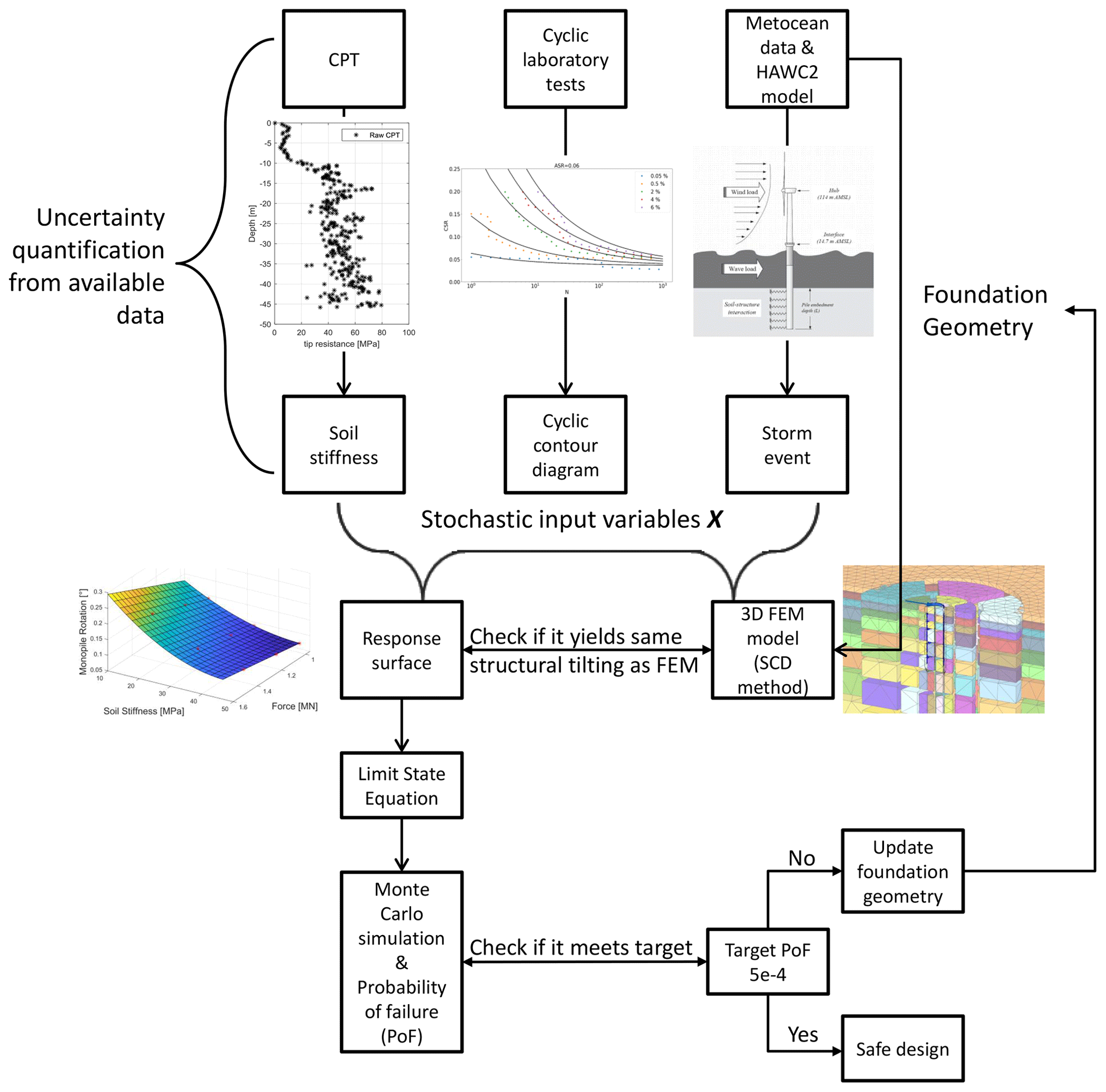
Figure 1 summarizes the methodology for the reliability analysis design for lateral cyclic loading. The framework starts with the uncertainty quantification from the available data (CPT, cyclic laboratory tests of the soil, and metocean and aero-hydro-servo-elastic model) and the derivation of the stochastic input variables (soil stiffness, cyclic contour diagram and storm event). The chosen stochastic variables are the inputs of the SCD model. Based on the stochastic input variables, a response surface is then trained to yield the same output (in terms of structural tilting) of the 3D FE simulations. The response surface is then used to calculate the probability of failure passing through the formulation of the limit state equation and the MC simulation. If the calculated probability of failure does not meet the target probability, then the foundation geometry has to be changed, and the methodology is repeated to check whether the new design is safe.
In this section, firstly, the monopile pre-design (static load design step) is carried out in which the subsoil conditions of the case study and the ULS design of the monopile geometry supporting a 10 MW wind turbine are explained. The pre-design of the monopile is developed using the hardening soil model in finite-element model to predict the static response of the monopile.
Then the reliability framework for the cyclic load design shown in Fig. 1 is applied to the monopile to check if the pre-design satisfies the SLS criteria. The following subsections discuss the derivation of input uncertainties for the SCD method, derivation of the response surface and probability of failure, and reliability index calculation.
3.1 Monopile pre-design: subsoil condition and pile geometry
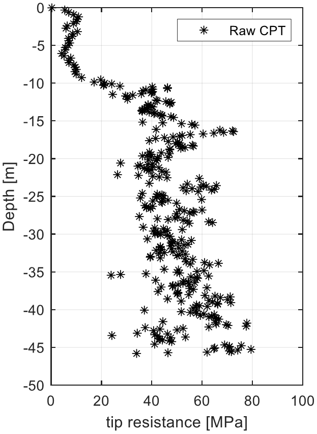
For the present case study, a tip resistance from the cone penetration test (CPT) and the boring profile are used to determine the geotechnical properties and soil stratigraphy at the site, where the monopile is assumingly installed. A CPT is basically a steel cone which is pushed into the ground and the tip resistance is recorded. Based on the recorded tip resistance, soil stratigraphy and soil properties can be empirically derived.
The CPT, shown in Fig. 2, features an increase in the tip resistance with increasing depth, which is typical for sand. In combination with the borehole profile, the tip resistance from the CPT suggests that the soil can be divided into two different layers. At approximately −10 m there is a jump in the tip resistance marking a transition to another layer with a higher magnitude visible, leading to the conclusion that denser sand is present. The characterization of the soil extracted from the boreholes shows the first layer (from 0 to −10 m) consisting of fine to medium sand and the second layer (from −10 m) consisting of well-graded sand with fine gravel.
To accurately predict the soil–structure interaction and incorporate the rigid behaviour of the large-diameter monopile, the ULS geotechnical verification of the preliminary design of the monopile is carried out, using the finite-element method in PLAXIS 3D.
The monopile is modelled in PLAXIS as a hollow steel cylinder using plate elements. For the steel, a linear elastic material is assumed with a Young's modulus of 200 GPa and a Poisson coefficient of 0.3. The interface elements are used to account for the reduced shear strength at the pile's surface.
The soil model used is the hardening soil model with small-strain stiffness (HSsmall) (PLAXIS, 2017). The hardening soil model with small strain stiffness can predict the non-linear stress–strain behaviour of the soil. It considers a stress and strain stiffness dependency, can predict the higher stiffness of the soil at small strain which is relevant for cyclic loading condition, and distinguishes between loading and unloading stiffness.
On the other hand, the Mohr–Coulomb model approximates the complex non-linear behaviour of the soil by a linear-elastic perfectly plastic constitutive law.
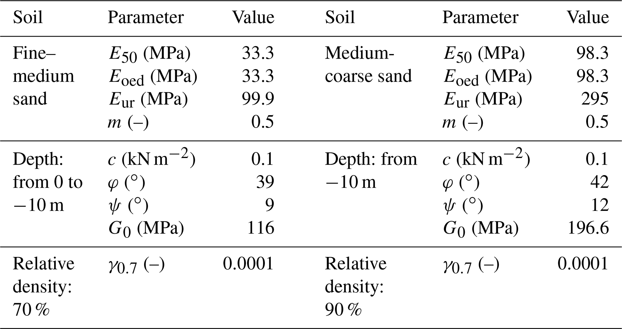
The soil model parameters for the two layers are derived from the tip resistance (Fig. 2) and listed in Table 1. The relative density (which is related to the soil porosity) of the two layers is calculated using the formula from Baldi et al. (1986) with the over-consolidated parameters (typical for offshore conditions), leading to a mean value of 70 % and 90 % for the first and second layers, respectively.
The monopile design requires a loop between the structural and geotechnical engineers to update the soil stiffness and loads at the mud-line level. A fully coupled aero-hydro-servo-elastic model using HAWC2 (Larsen and Hansen, 2015) is developed to perform the time-domain wind turbine load simulations (Velarde et al., 2020). The soil–structure interaction model is based on the Winkler-type approach, which features a series of uncoupled non-linear soil springs (so called p−y curves) distributed every 1 m. The force (p) − deformation (y) relations are extracted from the PLAXIS 3D model. At each meteor section, the calculation of the force (p) is carried out by integrating the stresses along the loading direction over the surface. The displacement (y) is taken as the plate's displacement. The PISA project (Byrne et al., 2019) highlights that additional soil reaction curve components (distributed moment, horizontal base force and base moment) are needed in conjunction with the p−y curves in order to have a more accurate soil structure interaction behaviour. For the sake of simplicity, only the p−y curves extracted from the FE model are considered.
The final pile design consists of an outer pile diameter at the mud-line level of 8 m a pile thickness of 0.11 m, and a pile embedment length of 29 m. The natural frequency of the monopile is 0.20 Hz and is designed to be within the soft-stiff region. Fatigue analysis of the designed monopile is also carried out (Velarde et al., 2020). Figure 3a shows the horizontal displacement contour plot at 3.5 MN horizontal force, while Fig. 3b shows the horizontal load-rotation curve at the mud-line.

Figure 3(a) Horizontal displacement contour plot at 3.5 MN horizontal load; (b) monopile rotation.
3.2 Input uncertainties for the SCD model
The application of the SCD model requires three inputs – soil stiffness (for the Mohr–Coulomb soil model), cyclic contour diagrams and a design storm event. The laboratory testing and field measurements are used to estimate the inputs for the model. In this estimation process, different sources of uncertainty of unknown magnitude are introduced (Wu et al., 1989). These parameters then have to be modelled as stochastic variables with a certain statistical distribution.
3.2.1 Soil stiffness
The uncertainties of the soil stiffness used in the SCD model are analysed. The soil model employed in the SCD method is the Mohr–Coulomb model, with a stress-dependent stiffness (i.e. the stiffness increases with depth). For cyclic loading problems, the unloading–reloading Young's modulus Eur is used. This soil modulus is obtained from the tip resistance from the CPT test (Fig. 2). The layering of the soil domain is assumed to be deterministic as explained in Sect. 3.1.
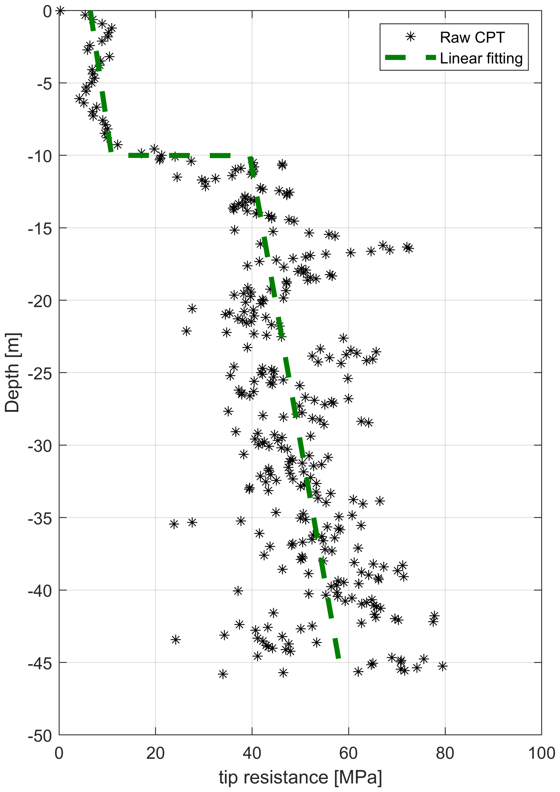
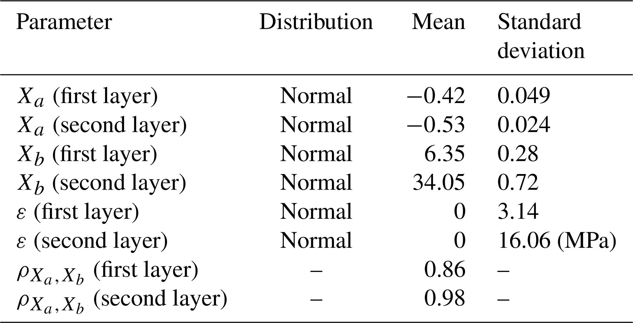
The design tip resistance is established by means of the best-fit line in the data. A linear model is fitted to the data for each layer (Fig. 4, green line). The maximum likelihood estimation (MLE) is used for estimating the parameters of the linear model along with the fitting error (assumed to be normally distributed and un-biased). From the MLE method, the standard deviations and correlations of the estimated parameters (Sørensen, 2011) are obtained. The linear model is expressed by means of Eq. (5) as below:
where Xa and Xb are stochastic variables modelling parameter uncertainty related to the parameters a and b, respectively; ε is the fitting error; and z is the depth (m). Table 2 shows a summary of the fitting parameters.
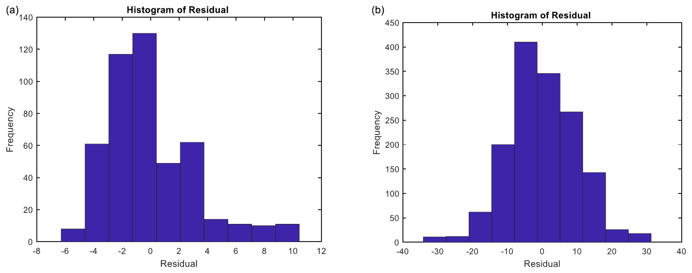
The residuals are then plotted to check the assumption of the normality of the model error. For the first layer (Fig. 5a), the distribution of the residual is slightly skewed to the right. This means that the trend line under-represents the tip resistance due to the presence of high peaks at the boundary layer. For the second layer (Fig. 5b), a normal distribution about the zero mean is visible, implying that a better fit is achieved.
An empirical linear relationship is used to calculate the drained constraint modulus in unloading–reloading Es (Lunne et al., 1997; Lunne and Christoffersen, 1983):
where Xα is a unitless stochastic variable. For over-consolidated sand, which is typical of offshore conditions, a value of α=5 is recommended (Lunne and Christoffersen, 1983). However, there is no unique relation between the stiffness modulus and the tip resistance because the α value is highly dependent on the soil, stress history, relative density, effective stress level and other factors (Lunne et al., 1997; Bellotti et al., 1989; Jamiolkowski et al., 1988).
To understand the uncertainty in the stiffness modulus, α is treated as a stochastic normal variable varying from αmin=3 to αmax=8 with a mean μ=5.5 and standard deviation σ=1.25. The standard deviation is calculated by , assuming that 95.4 % of the values are enclosed between the α values of 3 and 8.
Thus, the calculation of the drained constraint modulus in unloading–reloading, covering all possible uncertainties, is summarized as follows:
Depending on the size of the foundation, the local fluctuation (physical uncertainty) of the tip resistance can have a significant impact on the structural behaviour. If the size of the foundation is large enough, the soil behaviour is governed by the average of the global variability of the tip resistance (mean trend value). For a smaller foundation, the local effect, i.e. the local physical variability of the tip resistance, governs the soil behaviour. If the local variability of the tip resistance does not affect the foundation behaviour compared to the fitted linear model, it can be neglected. Moreover, the uncertainty related to the empirical formulation for calculating the soil stiffness (Xα) has a higher influence compared to the one used to approximate the tip resistance with a linear model (XaXbε). The preliminary results show that the uncertainty associated with approximating the tip resistance with the mean trend line is negligible due to the size of the monopile. For this reason, XaXbε values are considered deterministic at their mean value.
Figure 6 shows the variability of the soil modulus Es over depth. The red lines are the realizations, using the MC simulation by performing random sampling on the stochastic variable Xα. The black points are the deterministic multiplication of the tip resistance with a mean value of α=5.5.
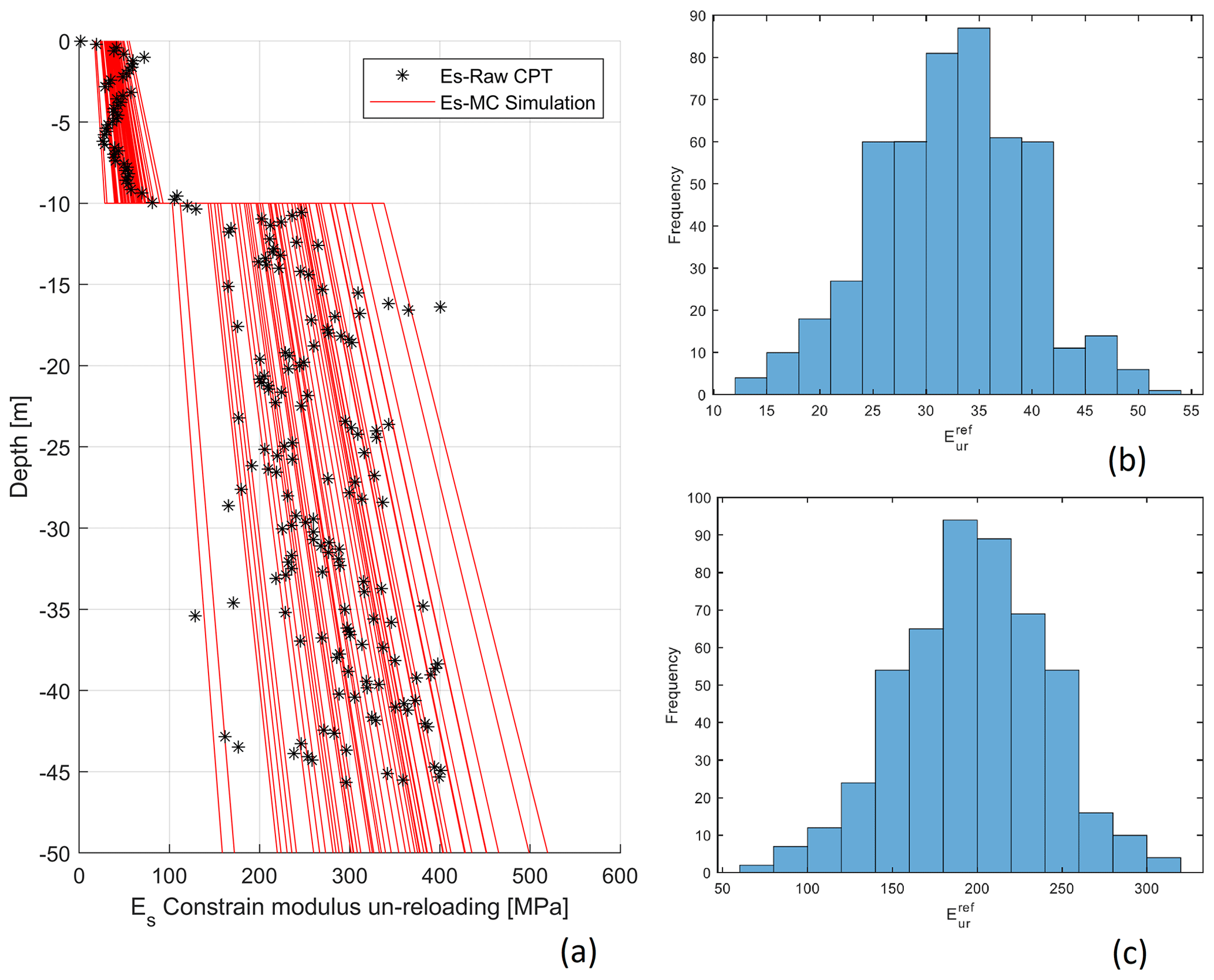
Figure 6(a) Variability of the soil modulus Es over depth; (b) histogram of the soil stiffness at zref=0 m; (c) histogram of the soil stiffness at m.
The drained constraint modulus in unloading–reloading Es is then converted to the drained triaxial Young's modulus in unloading–reloading Eur used in the Mohr–Coulomb soil model in PLAXIS. Assuming an elastic behaviour of the soil during unloading–reloading, Es and Eur can be related as
where υur is the Poisson ratio (=0.2).
The soil stiffness depends on the depth. In the Mohr–Coulomb model, a linear increase in the stiffness with depth is accounted for using the following formula:
where E(z)ur is the Young's modulus for unloading–reloading at a depth z, is the Young's modulus for unloading–reloading at a reference depth zref and Einc is the increment of the Young's modulus. Using this equation for a given input value of and the increment Einc, Eur can be derived at a specific depth below the surface and compared to Es, as specified in the design soil profile. For all realizations of different soil stiffness values (Fig. 6 red lines), and the increment Einc are calculated:
-
for the first layer at zref=0 (Fig. 6b): MPa and MPa;
-
for the second layer at m (Fig. 6c): MPa and MPa.
Other soil properties, such as specific weight, friction angle and relative density are considered to be deterministic. A full positive correlation between the two soil layer stiffness values is assumed.
3.2.2 Cyclic contour diagrams
The aim of the contour diagrams is to provide a 3D variation in the accumulated permanent strain in the average stress ratio (ASR), which is the ratio of the average shear stress to the initial vertical pressure or confining pressure; the cyclic stress ratio (CSR), which is the ratio of the cyclic shear stress to the initial vertical pressure or confining pressure; and the number of cycles (N). An extensive laboratory test campaign is needed to have an accurate 3D contour diagram. The laboratory campaign generally consists of carrying out different regular cyclic load tests with different average and cyclic amplitude stresses for a certain number of cycles.
For this work, a series of undrained single-stage two-way cyclic simple shear tests were performed at the Soil Mechanics Laboratories of the Technical University of Berlin. The tests were carried out on reconstituted soil samples. The samples were prepared by means of the air pluviation method. The initial vertical pressure was 200 kPa and no pre-shearing was considered.
The cyclic behaviour of the upper layer of sand was evaluated with samples prepared at a relative density of 70 %. For the lower layer sand, a 90 % relative density was used. Two-way cyclic loading tests were carried out, testing different combinations of ASR and CSR. All the tests were stopped at 1000 cycles or at the start of the cyclic mobility phase. For the results on the cyclic behaviour of various tests and relative densities, refer to Zorzi et al. (2019b).
All the data extracted from the laboratory tests were assembled in a 3D matrix (ASR, CSR, N), and a 3D interpolation of the permanent shear strain (γp) was created to map the entire 3D space. The repeatability of the cyclic simple shear tests is an important aspect to consider in evaluating the uncertainties in the cyclic contour diagram. Cyclic simple shear tests feature a low repeatability for dense sand, which can be attributed to the relatively small specimen size used for testing (Vanden Bergen, 2001). This makes the cyclic tests sensitive to sample preparation, resulting in, for example, different initially measured relative densities, soil fabric and void ratio non-uniformities.
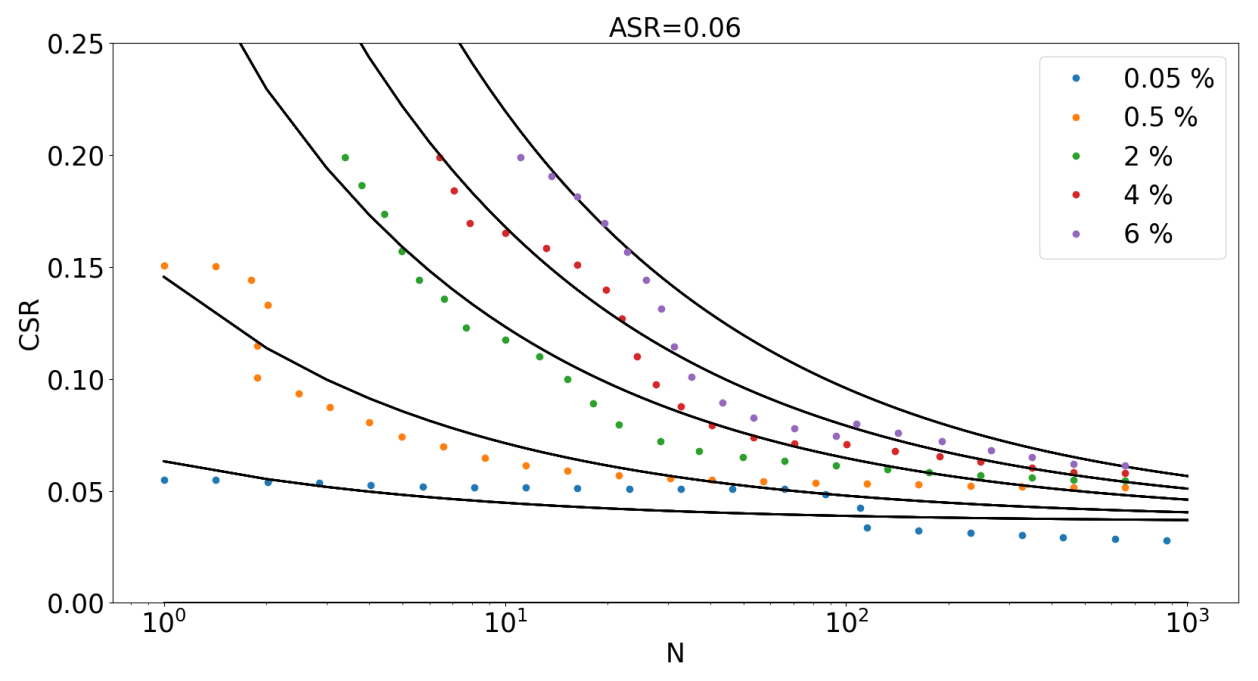
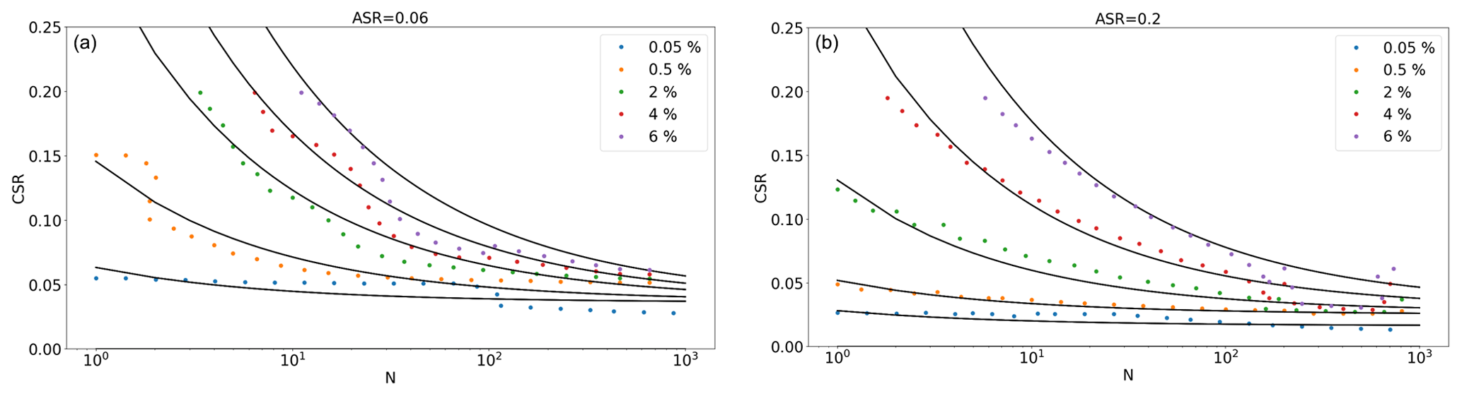
Owing to this variability of the test, a mathematical formulation was fitted to the raw interpolation. For this reason, different two-dimensional slices (CSR vs. N) at different ASR values were extracted. Figure 7 represents a slice of ASR equal to 0.06. The different coloured points represent the strain surfaces γp for different levels of deformation. The raw interpolation of data and the uncertainty related to the low sample repeatability of the tests cause an unrealistic non-smooth shape of the strain surfaces. Therefore, each slice is assumed to follow a power-law function (variation in CSR as power of N) for different strain levels and then calibrated to fit the data. Finally, the calibrated strain surfaces are interpolated to create the final smooth 3D contour diagram. This procedure and its validation are explained in Zorzi et al. (2019a).
The power-law function can be written in the form of Eq. (1).
where Xd represents the shape of the curve, Xc is a scaling factor, Xe is the intersection with the CSR axis and ε is the fitting error. Using the maximum likelihood method (MLM) it is possible to fit the mathematical model and estimate the standard deviation of the fitting error and the standard deviation of the parameters c and e. During the fitting procedure, the shape parameter d is assumed fixed at −0.35 for the lower layer and −0.50 for the upper layer.
Based on the results of the fitting procedure, a standard deviation of the fitting error of 0.008 is chosen for the two diagrams for the two soils. The parameters c and e are considered deterministic, as the associated standard deviation is very low. Preliminary simulations show that the uncertainty of a and c derived from the MLM has less influence than the uncertainty in the fitting error.
It has to be noted that the fitting error, to some extent, reflects the uncertainties of repeatability of the tests. Moreover, the relative density of the soil samples is based on the empirical relation applied to the tip resistance (Sect. 3.1). To account for the uncertainty in the relative density, different sets of contour diagrams should have been derived from several tests performed with soil samples at different relative densities.
The contour diagrams for two different ASR slices are presented in Figs. 8 and 9 for the upper and lower layers, respectively.

3.2.3 Load uncertainty
The load input parameter for the SCD model is characterized by a regular loading package with a mean and cyclic amplitude load and an equivalent number of cycles (hereafter called “load inputs” for simplicity). In common practice, the structural engineer provides the irregular history at mud-line level by means of the aero-hydro-servo-elastic model. Therefore, a procedure is needed to transform the irregular design storm event to one single regular loading parcel. The environmental load used for the cyclic loading design relies on the chosen return period for the load. The statistical distribution of the environmental loads is then based on different return periods.
The design storm event is here defined as a 6 h duration of the extreme load (also called the peak of the storm) (DNV-GL, 2017). The underlying assumption in considering only the peak is that most of the deformations, which the soil experiences, happen at the peak of the storm. The considered design load case is DLC 6.1 (IEC, 2009; BSH, 2015), i.e. when the wind turbine is parked and yaw is out of the wind. The ULS loads are considered for the cyclic load design.
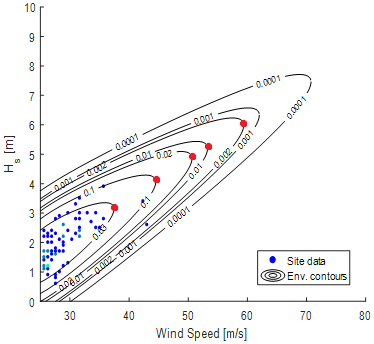
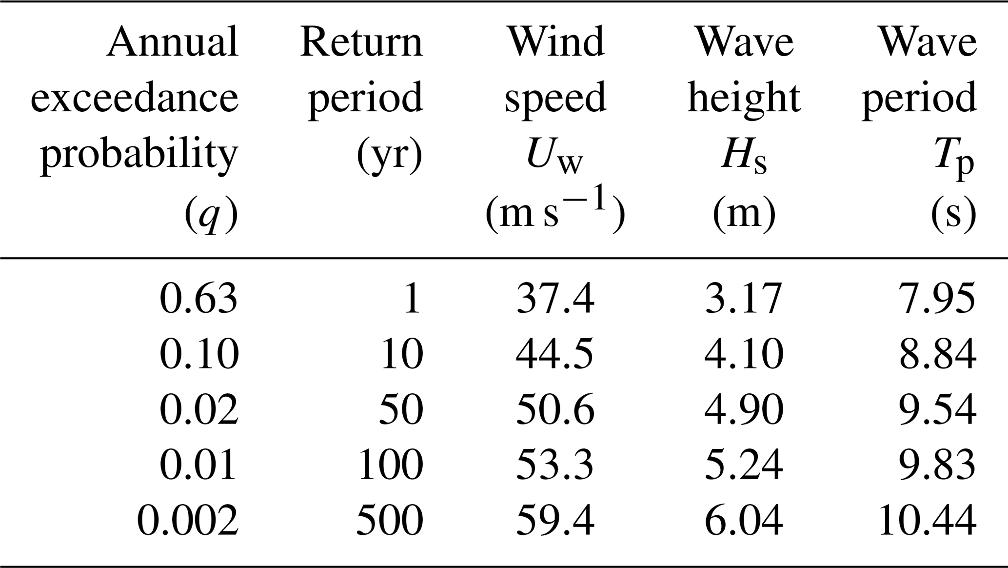
To derive the irregular load history at the mud-line level, the fully coupled aero-hydro-servo-elastic model is developed in the wind turbine simulation tool, HAWC2. Based on 5-year in situ metocean data from the North Sea, the environmental contours for different return periods are derived as shown in Fig. 10 (Velarde et al., 2019). The marginal extreme wind distribution is derived using the peak-over-threshold method for wind speed above 25 m s−1. Furthermore, it is assumed that maximum responses are given by the maximum mean wind speed and conditional wave height for each return period (red point in Fig. 10).
The five design sea states for maximum wind speed are summarized in Table 3. To account for short-term variability in the responses, 16 independent realizations are considered for each design sea state.
Time-domain simulations provide an irregular force history of 10 min at the mud-line. To transform the 10 min irregular loading to a 6 h storm, each 10 min interval is repeated 36 times.
The irregular load histories have to be simplified to one equivalent regular package with a specific mean and cyclic load amplitude and an equivalent number of cycles that lead to the same damage accumulation (accumulation of soil deformation) as that of the irregular load series.
The following procedure is used (Andersen, 2015).
-
The rain flow counting method is utilized to break down the irregular history into a set of regular packages with different combinations of mean force Fa and cyclic amplitude force Fcly and number of cycles N. Figure 11 shows an example of the output from the rain flow counting.
-
All the bins are ordered with increasing maximum force Fmax obtained from the sum of the mean and the cyclic amplitude ().
-
3D contour diagrams in conjunction with the strain accumulation method are then used to calculate the accumulation of deformation. After scaling the loads to shear stresses, the result of this procedure gives the equivalent number of cycles for the highest maximum force , which in turn gives the same accumulation of deformation of the irregular load history.
This procedure is applied for all simulations with different return periods.

To obtain a statistical distribution, the mean force, cyclic amplitude force and equivalent number of cycles are plotted versus the probability of non-exceedance for each return period.
The black points in the three following figures are, respectively, the mean load, cyclic amplitude and number of cycles of the regular packages obtained from the previous procedure and plotted vs. the probability of not exceedance for each return period. Assuming that for each return period the black points have a normal distribution, the 0.50 fractile (red circles) and the 0.95 fractile (blue circles) are obtained.
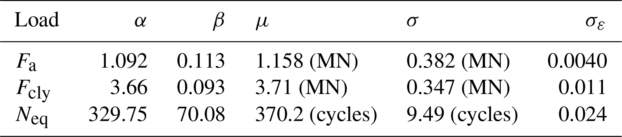
The statistical distributions for the loads are derived by fitting a Gumbel distribution to the 0.95 fractile values (NORSOK, 2007). The MLM is employed to fit the cumulative Gumbel distribution to the extreme response (blue circles). The cumulative density function distribution is defined as
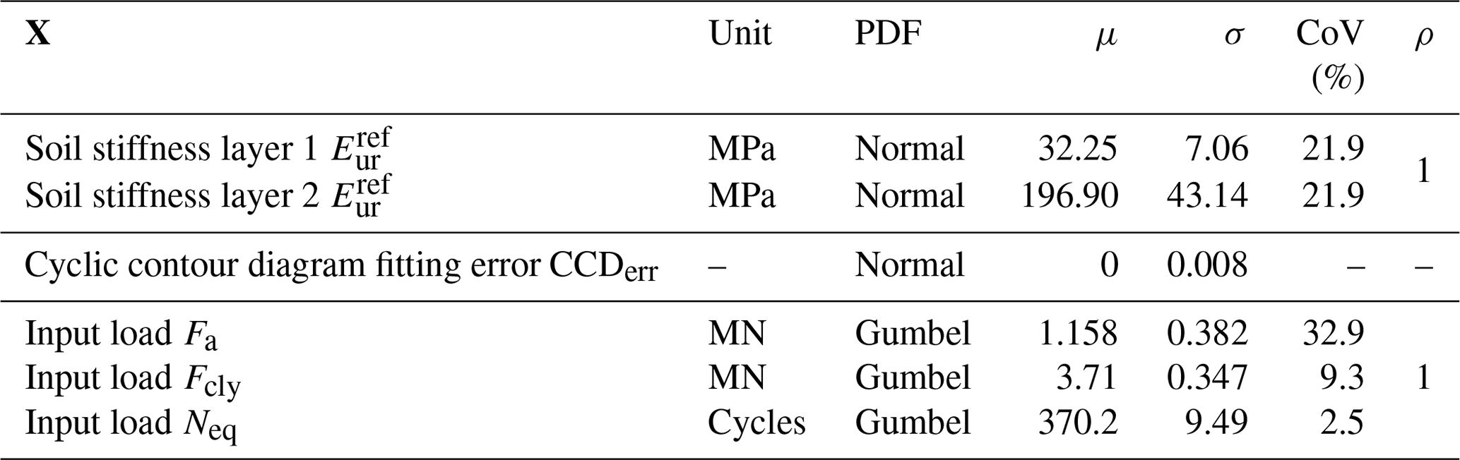
The Table 4 summarizes the parameters of distribution for the three load inputs. The standard deviation of the fitting error is small, marking a good fitting of the distribution function.
Table 4Gumbel parameters of the distribution for the load inputs.
Looking at the distribution of Fig. 12a–c, larger 0.50 fractiles (red circles) are present when increasing the return period. This is more pronounced for the mean force and is expected because the higher the return period, the higher the mean pressure on the wind turbine tower.
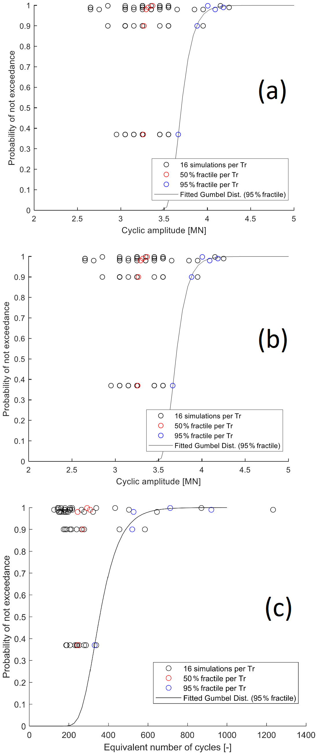
The scatter for each return period is more significant when the return period increases. This can have different reasons; for example, the “rare” storms with a lower probability of occurrence could cause more non-linearity problems, varying the wave and wind speeds in the aero-hydro-servo-elastic model. It could also depend on the model uncertainty in the time domain simulations.
The correlation coefficients ρ for the 0.95 fractile values between the mean and cyclic loads and the equivalent number of cycles are , and . The three coefficients mark a strong positive correlation between the three load inputs.
3.2.4 Model error
This type of error is difficult to estimate because it requires the validation of the numerical error against different model tests. In the case of the SCD model, this error arises due to the simplification of the model for a much more complex behaviour of the soil–structure interaction under cyclic loading. The model error εmodel is estimated as a random variable and multiplied to predict the structural tilting (Eq. 14). The model error is assumed to be normally distributed with a unitary mean and a coefficient of variation of 10 %. Ideally, this model uncertainty should be quantified comparing the results from the SCD model with several different test results. However, such a large number of tests is not feasible.
3.3 Derivation of the response surface
The stochastic variables are summarized in Table 5. For simplicity, a full correlation between the soil stiffness of the two layers and the loads is assumed.
Once the stochastic variables are defined, the 3D FE model has to be substituted by a response surface.
The DoE is used to obtain the training point from the FE simulation. As most of the variables are correlated, three stochastic variables are considered: (i) the stiffness of the upper soil layer Eur, (ii) the fitting error of the cyclic contour diagram CCDerr and (iii) the mean load Fa. The independent input stochastic variables have the statistical distribution shown in Table 5. For each factor, three different levels are assumed: minimum value , average value μ and maximum value . A full factorial design in three levels is implemented. Therefore, a total of 33 simulations are needed to explore all possible combinations.
Based on visual inspection of the output from the 3D FE model, a second-order polynomial function is fitted to the sample data. The linear regression method is used to estimate regression coefficients of the polynomial function. The following function is the outcome of the linear regression analysis:
An un-biased fitting error (ε) with normal distribution is assumed and the estimate of residual standard deviation () is 0.0013. R-squared is a statistical measure of how close the data are to the fitted regression line. For the fitted function, the R-squared value is 0.9984, underlining a good fit of the function to the data and hence the choice of the initial choice of the second-order polynomial function.
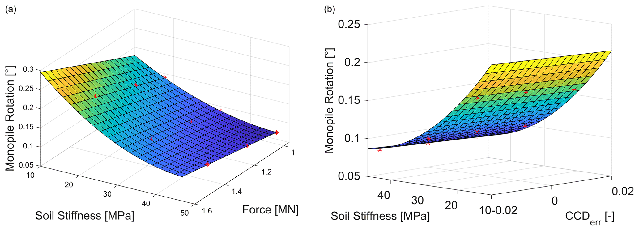
Figure 13a shows the function at the CCDerr=0 (the mean value). The surface shows that at a lower soil stiffness and a high force, a higher rotation of the monopile is reached. Values higher than 0.25 are considered failures. The red points are from the numerical simulations. The 3D plot (Fig. 13b) shows the response surface for the mean value of the force Fa=1.158 MN. It is apparent that the fitting error for the contour diagram is small and thus does not have a significant influence on the results.
3.4 Reliability analysis
The limit state function is written as
A total of 107 MC simulations were performed by random sampling of the input stochastic variables. This number was the minimum required to keep the relative error of the reliability index lower than 1 %. The stochastic variables and their probability distribution functions are given in Table 5. The derivation of the design mean and standard deviation are explained in Sect. 3.2.
With the analysed monopile design, the annual probability of failure is and the corresponding annual reliability index is 4.03. This means that the monopile meets the target reliability index of 2.9–3.3 and is considered safe for long-term behaviour in terms of rotation accumulation for the design storm event.
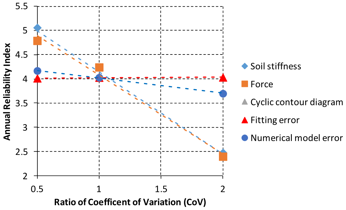
3.5 Sensitivity analysis
The sensitivity analysis of the stochastic input variables on the reliability index is conducted by varying the coefficient of variation one at a time for each input (0.5 and 2 coefficient of variation, CoV). The inclination of dashed lines in Fig. 14 marks the sensitivity of the stochastic variable. Mean force Fa and the soil stiffness Eur both influence the reliability index significantly more than the fitting error and numerical model error do.
During the lifetime of wind turbines, storms, typhoons or seismic action are likely to cause permanent deformation of the structure owing to the accumulation of plastic strain in the soil surrounding the foundation. The serviceability limit state criteria require that the long-term structural tilting does not exceed the operational tolerance prescribed by the wind turbine manufacturer (usually less than 1∘) with a specific target reliability level. In this study, the SLS design for long-term structural tilting is addressed within a reliability framework. This framework is developed based on the 3D FE models for the prediction of the SSI under cyclic loading. For the case study of a large monopile installed on a typical North Sea environment, a reliability index of 4.03 was obtained. Sensitivity analysis also shows that uncertainties related to the soil stiffness and the environmental loads significantly affect the reliability of the structure. For regions where assessment against accidental loads due to typhoons is necessary, uncertainty of the extreme environmental loads can increase by up to 80 %. Such load scenarios can significantly reduce the reliability index and therefore become the governing limit state.
A discussion has to be started in the offshore community regarding the very strict tilting requirement (i.e. 0.25∘). This very small operational restriction can lead to foundations of excessively large dimensions, which are unfeasible from an economic point of view. On the other hand, a less strict verticality requirement (which could be a function of the dimension and type of the installed wind turbine), for example an angle of rotation of 1–3∘, could lead to a smaller foundation size and still meet the safety requirements. For this reason, by means of aero-elastic analyses, the investigation of the position of the natural frequency of the whole system and fatigue analysis should be carried out when a wind turbine is tilted at 1–3∘. Allowing a less stringent tilting of the foundation can also be beneficial during the monopile installation. A small foundation dimension saves vessel and equipment cost, which contributes significantly to the overall cost reduction of the foundation.
In this paper, a simplified model to calculate the permanent rotation (the SCD method) is implemented. It is noted that other models of varying complexity can also be used in the proposed probabilistic framework. If new inputs are introduced, the respective uncertainties should be considered in the reliability calculation and the function for the response surface should be adjusted accordingly.
The codes can be made available by contacting the corresponding author.
GZ, AM, JV and JDS designed the proposed methodology. GZ prepared the manuscript with the contributions from all co-authors.
The authors declare that they have no conflict of interest.
This article is part of the special issue “Wind Energy Science Conference 2019”. It is a result of the Wind Energy Science Conference 2019, Cork, Ireland, 17–20 June 2019.
This research is part of the Innovation and Networking for Fatigue and Reliability Analysis of Structures – Training for Assessment of Risk (INFRASTAR) project. This project has received funding from the European Union's Horizon 2020 Research and Innovation programme under the Marie Skłodowska-Curie grant agreement no. 676139. The laboratory tests are provided by Chair of Soil Mechanics and Geotechnical Engineering of the Technical University of Berlin. The authors are grateful for the kind permission to use those test results.
This research has been supported by the Innovation and Networking for Fatigue and Reliability Analysis of Structures – Training for Assessment of Risk (INFRASTAR) (grant no. 676139).
This paper was edited by Athanasios Kolios and reviewed by Federico Pisano and one anonymous referee.
Achmus, M., Abdel-Rahman, K., and Kuo, Y.: Behaviour of large diameter monopiles under cyclic horizontal loading, in: Twelfth International Colloquium on Structural and Geotechnical Engineering, 10–12 December 2007, Cairo, Egypt, 2007.
Andersen, K. H.: Cyclic soil parameters for offshore foundation design, in: Frontiers in Offshore Geotechnics III, ISFOG'2015, 10–12 June 2015, Oslo, Norway, 5–82, ISBN 978-1-138-02848-7, 2015.
Baldi, G., Bellotti, R., Ghionna, V., Jamiolkowski, M., and Pasqualini, E.: Interpretation of CPTs and CPTUs; 2nd part: drained penetration of sands, in: Proc. 4th Int. Geotech. Seminar, Singapore, 143–156, 1986
Bellotti, R., Ghionna, V. N., Jamiolkowski, M., and Robertson, P. K.: Design parameters of cohesionless soils from in situ tests, Transport. Res. Rec., 1235, 45–54, 1989.
Bhattacharya, S.: Challenges in Design of Foundations for Offshore Wind Turbines, Eng. Technol. Ref., 9, 1–9, https://doi.org/10.1049/etr.2014.0041, 2019.
BSH: Standard Design – minimum requirements concerning the constructive design of offshore structures within the Exclusive Economic Zone (EEZ), Federal Maritime and Hydrographic Agency (BSH), Federal Maritime and Hydrographic Agency (BSH), Hamburg, Rostock, 2015.
Byrne, B. W., Burd, H. J., Zdravkovic, L., Abadie, C. N., Houlsby, G. T., Jardine, R. J. and Taborda, D. M. G.: PISA Design Methods for Offshore Wind Turbine Monopiles, in: Offshore Technology Conference, 6–9 May 2019, Houston, Texas, https://doi.org/10.4043/29373-MS, 2019.
Carswell, W. Arwade, S., DeGroot, D., and Lackner, M.: Soil–structure reliability of offshore wind turbine monopile foundations, Wind Energy, 18, 483–498, https://doi.org/10.1002/we.1710, 2014.
Cuéllar, P., Georgi, S., Baeßler, M., and Rücker, W.: On the quasi-static granular convective flow and sand densification around pile foundations under cyclic lateral loading, Granular Matter, 14, 11–25, https://doi.org/10.1007/s10035-011-0305-0, 2012.
DNV-GL: DNVGL-RP-C212 – Offshore soil mechanics and geotechnical engineering, DNV GL AS, 2017.
Fenton, G. and Griffiths, D.: Risk assessment in geotechnical engineering, John Wiley & Sons, Inc., Hoboken, NJ, USA, https://doi.org/10.1002/9780470284704, 2008.
Hettler, A.: Verschiebungen starrer und elastischer Gründungskörper in Sand bei monotoner und zyklischer Belastung, Institut für Bodenmechanik und Felsmechanik der Universität Fridericiana, Karlsruhe, 1981.
IEC: IEC 61400-3 - Wind turbines Part 3: Design requirements for offshore wind turbines, International Electrotechnical Commission, Geneva, 2009.
Jamiolkowski, M., Ghionna, V., Lancellotta, R., and Pasqualini, E.: New correlations of penetration tests for design practice, Int. J. Rock Mech. Mining Sci. Geomech., 27, A91, https://doi.org/10.1016/0148-9062(90)95078-f, 1988.
Jostad, H. P., Grimstad, G., Andersen, K. H., Saue, M., Shin, Y., and You, D.: A FE Procedure for Foundation Design of Offshore Structures – Applied to Study a Potential OWT Monopile Foundation in the Korean Western Sea, Geotech. Eng. J., 45, 63–72, 2014.
Larsen, T. J. and Hansen, A. M.: How 2 HAWC2, the user's manual, Risø National Laboratory, Technical University of Denmark, Roskilde, Denmark, 2015.
LeBlanc, C., Houlsby, G. and Byrne, B.: Response of stiff piles in sand to long-term cyclic lateral loading, in: Geotechnique, Band 602, ICE Publishing, 2009.
Lunne, T. and Christoffersen, H. P.: Interpretation of Cone Penetrometer Data for Offshore Sands, in: Offshore Technology Conference, 2–5 May 1983, Houston, Texas, https://doi.org/10.4043/4464-MS, 1983.
Lunne, T., Robertson, P. K., and Powell, J. J. M.: Cone Penetration Testing in Geotechnical Practice, CRC Press, London, https://doi.org/10.1201/9781482295047, 1997.
Niemunis, A., Wichtmann, T., and Triantafyllidis, T.: A high-cycle accumulation model for sand, Comput. Geotech., 32, 245–263, https://doi.org/10.1016/j.compgeo.2005.03.002, 2005.
NORSOK: NORSOK Standard N-003, Actions and action effects, Standards Norway, Lysaker, Norway, 2007.
Pisanò, F.: Input of advanced geotechnical modelling to the design of offshore wind turbine foundations, in: Proceedings of the XVII ECSMGE-2019: Geotechnical Engineering foundation of the future, 1–6 September 2019, Reykjavik, Iceland, https://doi.org/10.32075/17ECSMGE-2019-1099, 2019.
PLAXIS: Plaxis 3D Reference Manual, edited by: Brinkgreve, R. B. J., Kumarswamy, S., Swolfs, W. M., and Foria, F., Plaxis B. V., Delft, the Netherlands, 2017.
Sørensen, J. D.: Notes in Structural Reliability Theory and Risk Analysis, Aalborg University, Aalborg, 2011.
Vanden Bergen, J. F.: Sand Strength Degradation within the Framework of Vibratory Pile Driving, PhD thesis, University Catholique de Louvain, Faculty of Applied Science Civil and Environmental Engineering Division, Louvain, 2001.
Velarde, J., Kramhøft, C., and Sørensen, J. D.: Reliability-based Design Optimization of Offshore Wind Turbine Concrete Structures, in: 13th International Conference on Applications of Statistics and Probability in Civil Engineering, 26–30 May 2019, Seoul, Korea, https://doi.org/10.22725/ICASP13.185, 2019.
Velarde, J., Sørensen, J. D., Kramhøft, C., and Zorzi, G.: Fatigue reliability of large monopiles for offshore wind turbines, Int. J. Fatig., 134, 105487, https://doi.org/10.1016/j.ijfatigue.2020.105487, 2020.
Wichtmann, T.; Soil behaviour under cyclic loading – experimental observations, constitutive description and applications, in: Habilitation thesis, KIT – Karlsruher Institut für Technologie, Karlsruhe, 2016.
Wu, T., Tang, W., Sangrey, D., and Baecher, G.: Reliability of Offshore Foundations-State of the Art, J. Geotech. Eng., 115, 157–178, https://doi.org/10.1061/(asce)0733-9410(1989)115:2(157), 1989.
Zorzi, G., Richter, T., Kirsch, F., Augustesen, A. H., Østergaard, M. U., and Sørensen, S. P.: Explicit Method to Account for Cyclic Degradation of Offshore Wind Turbine Foundations Using Cyclic Inter-action Diagrams, in: International Society of Offshore and Polar Engineers, 10–15 June 2018, Sapporo, Japan, ISOPE-I-18-271, 2018.
Zorzi, G., Kirsch, F., Richter, T., Østergaard, M., and Sørensen, S.: Validation of explicit method to predict accumulation of strain during single and multistage cyclic loading, in: Proceedings of the XVII ECSMGE-2019 – Geotechnical Engineering foundation of the future, 1–6 September 2019, Reykjavik, Iceland, 2019a.
Zorzi, G., Kirsch, F., Richter, T., Østergaard, M., and Sørensen, S.: Comparison of cyclic simple shear tests for different types of sands, in: 2nd International Conference on Natural Hazards & Infrastructure, 23–26 June 2019, Chania, Greece, 2019b.