the Creative Commons Attribution 4.0 License.
the Creative Commons Attribution 4.0 License.
 | 10 Nov 2020
Identification of airfoil polars from uncertain experimental measurements
Chengyu Wang
Filippo Campagnolo
A new method is described to identify the aerodynamic characteristics of blade airfoils directly from operational data of the turbine. Improving on a previously published approach, the present method is based on a new maximum likelihood formulation that includes errors in both the outputs and the inputs, generalizing the classical error-in-the-outputs-only formulation. Since many parameters are necessary to meaningfully represent the behavior of airfoil polars as functions of angle of attack and Reynolds number, the approach uses a singular value decomposition to solve for a reduced set of observable parameters. The new method is demonstrated by identifying high-quality polars for small-scale wind turbines used in wind tunnel experiments for wake and wind farm control research.
- Article
(1853 KB) - Full-text XML
- BibTeX
- EndNote


Most simulation models of wind turbine rotors, from the low to the high end of the fidelity spectrum, rely on polars, i.e., on the aerodynamic characteristics of the airfoils used on the blade. Clearly, irrespectively of its sophistication, the quality of the results that a simulation can deliver is bound to many details of the underlying mathematical model and numerical methods but also to the accuracy of the polars. Unfortunately, it is often difficult to have a precise knowledge of such a crucial ingredient. In fact, whereas polars are typically characterized by ad hoc experiments or simulations conducted on isolated airfoils, there are many reasons why the actual polars of a specific blade can differ from the nominal ones. To address this need, this paper describes a new procedure for the tuning of polars based on turbine operational data.
Airfoil polars are used for modeling the aerodynamics of rotors using lifting lines in conjunction with blade element momentum (BEM), free vortex wake (FVW), and computational fluid dynamic (CFD) models. BEM methods are routinely used for the aeroservoelastic analysis of wind turbines and provide most of today's industrial-level simulation capabilities for load analysis, design, and control development activities (Manwell et al., 2009; Burton et al., 2011; OpenFast, 2020). FVW methods (Sebastian and Lackner, 2012; Shaler et al., 2019) are not yet routinely used because of their higher computational costs but offer promising alternatives by removing some of the assumptions of BEM theory. On the higher end of the spectrum, the large-eddy simulation actuator line method (LES-ALM; Troldborg et al., 2007; Churchfield and Lee, 2012; Churchfield et al., 2012; Wang et al., 2019) is currently the main approach for the modeling of wakes, including the hot topic of wind farm control (Fleming et al., 2013; Gebraad et al., 2016).
In all of these approaches, a lifting line models the blade from the aerodynamic point of view. A generic lifting line is a three-dimensional curve running along the blade, which may be prebent and swept. The local chord, twist, airfoil type, and its relative position (for example, in terms of the chordwise offset of the aerodynamic center) are specified along the curve. The lifting line is attached to the structural model of the blade and moves with it following its travel around the rotor disk and its deformation. At each instant of time during a simulation, the local flow relative to a generic point of the lifting line can be computed. The local flow accounts for the wind inflow, for the motion of the blade, and for the local induction generated by the rotor, whose details depend on the specific aerodynamic model (BEM, FVW, or CFD). Given the local flow, the angle of attack of the airfoil and the Reynolds number can be readily obtained. This allows one to compute the lift, drag, and moment aerodynamic coefficients at that location along the blade, typically by interpolating within look-up tables that store the aerodynamic properties of the airfoil. Possible corrections are applied to take into account tip and root losses, unsteady aerodynamics, dynamic stall, Coriolis-induced delayed stall, and other effects, in turn producing the local aerodynamic force exerted on the blade at that location. By the principle of action and reaction, an equal and opposite force is applied to the flow, and, again depending on the specific formulation, this closes the loop between blade motion and fluid flow. A new estimate of the local flow is therefore produced, and the process is repeated until convergence.
For several years, the group of the senior author has been developing scaled and controlled wind turbine models for wind tunnel testing (Bottasso et al., 2014b; Bottasso and Campagnolo, 2020). Applications have considered both wind turbine (Bottasso et al., 2014b) and wind farm control (Campagnolo et al., 2016, 2020; Frederik et al., 2019). In addition to the collection of valuable data sets in the known, repeatable, and controllable environment of the wind tunnel, the development and validation of digital copies of these experiments have been main ambitions of this research effort. Both aeroelastic BEM (Bottasso et al., 2014b) and LES-ALM (Wang et al., 2019) models of the experiments have been developed, in the latter case including not only the wind turbines but also the wind tunnel and the passive generation of a sheared and turbulent flow. Results collected to date demonstrate an excellent ability of the simulation models in reproducing the experiments, including multiple wake interactions and conditions relevant to wind farm control (Wang et al., 2019, 2020a, b, c).
One crucial component of the simulation chain has been a method for estimating the polars directly from operational data of the turbines (Bottasso et al., 2014a). In fact, the blades of scaled wind turbine models operate in low Reynolds regimes, where even relatively small changes in the operating conditions can cause significant changes in the aerodynamic characteristics of the blade sections. In addition, given the small size of these models, even modest manufacturing imperfections and normal wear of the blades can lead to deviations from their nominal shape. Using the method of Bottasso et al. (2014a), the nominal airfoil polars are augmented with parametric correction terms, which are identified using a maximum likelihood (ML) criterion based on operational power and thrust measurements. These data points are collected on the turbine at various operating conditions, selected in order to span a desired range of angles of attack and Reynolds numbers. Since a large number of free parameters are necessary to represent the correction terms, the resulting problem is ill-posed, and the parameters are collinear. To address this issue, the original parameters are transformed into a new orthogonal set by using the singular value decomposition (SVD). Because the new parameters are uncorrelated with each other, one can select an observability threshold, discard the unobservable set, and solve only for the observable one. After having solved the identification problem, which is now well posed, the solution is mapped back onto the space of the original physical parameters.
Although this method works well in practice, it still suffers from assumptions that limit its effectiveness. Indeed, the classical ML formulation is based on an input–output model and assumes errors in the outputs only (Klein and Morelli, 2006; Jategaonkar, 2015). Following this approach, outputs differ from available measurements because of measurement errors and model deficiencies. However, errors are not explicitly accounted for in the inputs, which are assumed to be equal to their measured values. In the present context, inputs represent the operating conditions of the turbines, which are expressed by the ambient air density and wind speed, the rotor angular velocity, and the blade pitch setting. Errors in such quantities have a non-negligible effect on the outputs and should be taken into account in a rigorous statistical sense.
To address this issue, the present paper proposes a new general formulation of ML identification that includes errors both in the outputs and in the inputs. This generalized formulation leads to an optimization problem in the model parameters and the unknown model inputs, which can now differ from their measured values. The proposed method is again cast within the SVD-based reformulation of the unknowns to deal with the ill-posedness and redundancy of the parameters. The new formulation is applied to the identification of the polars of small-scale controlled wind turbines, developed to support wind farm control and wake research (Wang et al., 2019; Campagnolo et al., 2020; Frederik et al., 2019; Bottasso and Campagnolo, 2020). Results indicate that the new formulation delivers polars of superior quality with respect to the original error-in-the-outputs-only formulation. Specifically, the new polars were able for the first time to correctly predict the turbine power outputs in derated conditions, which had always defied previous efforts.
The paper is organized according to the following plan. Section 2 describes first the classical ML approach in Sect. 2.1 and its reformulation in terms of uncorrelated parameters in Sect. 2.2; Sect. 2.3 presents the novel ML method with errors in both outputs and inputs, while Sect. 2.4 discusses a way to take into account a priori information on the errors. Section 3 specializes the general formulation of Sect. 2.3 to the identification of the polars of scaled wind turbines. Finally, Sect. 4 presents the results, and conclusions are drawn in Sect. 5.
2.1 Classical maximum likelihood estimation with errors in the outputs
Consider a system described by the parametric model
where u∈ℝl are the inputs (or, in the present context, the operating conditions), p∈ℝn the model parameters, and y∈ℝm the outputs. In correspondence to the N inputs , , …, , N experimental measurements of the outputs are available and noted , , …, . Because of modeling and measurement errors, the experimental measurements are in general not identical to the outputs predicted by Eq. (1), a difference that can be quantified by the residual . The goal of the estimation problem is to find the model parameters p that minimize the residuals r.
A classical approach to this parameter estimation problem is the ML method (Klein and Morelli, 2006). The idea of maximum likelihood estimation is to find the parameters p that maximize the probability J of obtaining the measurement sample 𝒴, where J is written as
R being the residual covariance and wi a weight assigned to the ith residual. In this work, weights are introduced to account for the fact that not all operating conditions appearing in the sample 𝒰 might have the same importance. For example, it might happen that some ui's represent frequent typical operating conditions of the system, whereas others are less frequent or relevant conditions. It might then be desirable to better match these more frequent conditions than the less frequent ones. One way to achieve this behavior from the ML estimator is to assign weights to the residuals. The weights could be proportional to the relative frequency of each operating condition in the lifetime of the system or be inversely proportional to the distance of that operating condition to some nominal behavior, a concrete example of this latter case being explained later in the results section.
A robust implementation of this optimization problem is obtained by the following iteration (Klein and Morelli, 2006).
-
Assuming temporarily frozen parameters equal to p, minimize J with respect to R, which yields the following expression for the covariance matrix (Jategaonkar, 2015):
where .
-
Assuming a temporarily frozen error covariance R, solve the minimization problem
-
Return to step 1, and repeat until convergence.
In the following, alternating between steps 1 and 2 is termed a “major” iteration. The internal iterations necessary for the solution of the optimization problem at step 1 are termed in the following “minor” iterations.
2.2 Maximum likelihood estimation in terms of uncorrelated parameters
The estimation problem expressed by Eqs. (3) and (4) can be ill-posed because of low observability and collinearity of the unknowns. This is a classical difficulty in parameter estimation: on the one hand one would typically prefer a rich set of parameters that give ample freedom to adjust the behavior of a model in order to accurately match the measurements; on the other hand, it might be difficult – if not altogether impossible – to always guarantee that there is enough informational content in the measurements to correctly identify and distinguish the effects of each one of the unknown parameters.
Indeed, the well-posedness of the identification problem is associated with the curvature of the likelihood function with respect to changes in the parameters. Around a flat maximum, different values of the parameters yield similar values of the likelihood. A measure of the curvature of the solution space is provided by the Fisher information matrix (Jategaonkar, 2015). The inverse of this matrix is also useful because it bounds the variance of the estimates (Cramér-Rao bound) (Jategaonkar, 2015). Unfortunately, the Fisher information by itself does not offer a constructive way of reformulating a given ill-posed problem.
To overcome this difficulty, Bottasso et al. (2014a) proposed to transform the original physical parameters of the model into an orthogonal parameter space. This mapping is obtained by diagonalizing the Fisher matrix using the SVD. As the new variables are now statistically independent, one can readily select and retain in the analysis only the parameters that are associated with a sufficiently high level of confidence. Once the problem is solved, the uncorrelated parameters are mapped back onto the original physical space.
This approach enables one to solve an identification problem with many free parameters, some of which might be interdependent or not observable in a given data set. Furthermore, the SVD diagonalization reduces the problem size, retaining only the orthogonal parameters that are indeed observable. Finally, this approach reveals, through the singular vectors generated by the SVD, the interdependencies that may exist among some parameters of the model, which may provide useful insight into the problem itself.
A detailed description of the SVD-based version of ML identification is given in Bottasso et al. (2014a). The same formulation is used also in the present paper.
2.3 Maximum likelihood estimation with errors in the inputs and outputs
The standard formulation of the ML identification presented in Sect. 2.1 considers the presence of noise in the outputs y. Indeed, outputs are affected by measurement errors but also, being computed through a model, by the deficiencies of the model itself. Although errors in the outputs are typically the primary source of uncertainty in a parameter estimation problem, there are situations where significant errors may also be associated with the inputs u, which is the case of the present application. A formulation of ML that accounts for errors both in the outputs and inputs is presented next.
The parametric model described by Eq. (1) is expanded as
Because of modeling and measurement errors, the experimental output measurements y* are in general not identical to the model-predicted outputs y. Similarly, because of measurement errors and an imperfect realization of the operating conditions, the experimental inputs u* are in general not identical to the nominal ones u. These differences can be synthetically quantified by the residual , where now is an expanded vector that contains measurements of both outputs and inputs:
The goal of the estimation problem is to find the model parameters p and system inputs ui that maximize the probability of obtaining the measurements y* and u*. According to the maximum likelihood criterion, Eq. (4) becomes
and Eq. (3) is now
Instead of solving the problem in a monolithic fashion, the following iteration can be conveniently used:
-
Initialize p (see Sect. 2.4), and set , i=[1, N].
-
Calculate from Eq. (8).
-
Assuming temporarily frozen inputs ui, solve
This is formally identical to the classical error-in-the-outputs-only ML formulation, which can be solved by the SVD-based reformulation in terms of uncorrelated parameters (Bottasso et al., 2014a).
-
Assuming temporarily frozen parameters p, solve
These are N decoupled small sized problems, which return the values of the model inputs.
-
Return to step 2, and repeat until convergence.
This way the solution of the identification problem with input and output errors is obtained by using the classical error-in-the-outputs-only ML implementation (using Eq. 9), followed by a sequence of inexpensive optimizations to compute the model inputs (using Eq. 10). Notice that, as long as it converges, this iteration returns the same result as the monolithic solution of Eqs. (7) and (8).
2.4 Filtering of measurements based on a priori uncertainties
Often, a priori information on the expected uncertainties may be available. In such cases, the unknown true inputs ui can be bounded as
where Δu are the expected uncertainty bounds. This a priori information can be used to retain in the cost function J only those measurements for which the corresponding residual cannot be simply explained by the uncertainties expressed in Eq. (11) but must be due to the model parameters p.
To this end, notice first that the residual ri is a function of p and ui, i.e.,
Indicating the jth component of residual ri as , its maximum and minimum values for a given p are computed as
If the maximum and minimum have different signs, then lies somewhere within this range, and hence this residual component can be fully explained by input uncertainties. Therefore, it cannot drive meaningful changes in the parameters and should be neglected. Otherwise, this residual carries valuable information and should be retained. To account for this, a filtered residual is defined as
The a priori estimates are used to initialize the parameters p at step 1 of the iterative algorithm formulated in Sect. 2.3. A standard ML method is used for the initialization, considering only errors in the outputs and using Eqs. (3) and (4) where the residual components are replaced by the filtered ones . Filtering accelerates the optimization because it avoids meaningless tuning of parameters caused by measurement noise. Once this initial estimate of the parameters is obtained, it is further refined by considering the a posteriori effects of noise in inputs and outputs by stepping through points 2–5 of the algorithm. Residual filtering is not used further because it is based on a priori assumptions relying on knowledge of the measurement chain, which can only estimate bounds and might not reflect the actual noise effectively experienced for any given measurement.
In practice, a naive implementation of filtering can be very expensive. In fact, as the residual ri depends on p, one would have to recompute the optimization problems expressed in Eq. (13) each time the parameters are updated, which becomes prohibitively expensive.
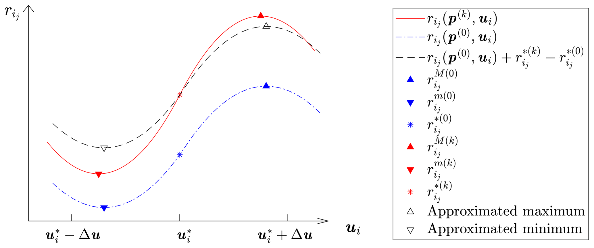
The cost of filtering can be drastically reduced with a simple approximation, as graphically illustrated in Fig. 1. The figure shows with a dotted blue line the residual component as a function of the input ui for a given value of the model parameters p(0). The counter (⋅)(0) refers to the values that the parameters assume at the beginning of each major iteration used to solve Eq. (4). The minimum and maximum of this curve, corresponding to and , are respectively indicated with downward- and upward-pointing blue triangles. These stationary points are computed at the beginning of each major iteration by solving Eq. (13). For simplicity, this is obtained by a simple evaluation of the residuals over a regular subdivision of the unknowns.
At the kth minor iteration of the solution of Eq. (4), the model parameters have been updated, and they now assume the value p(k). The corresponding function is depicted in the figure with a solid red line, together with its new minimum and maximum points indicated by downward- and upward-pointing red triangles. To reduce the computational burden, these stationary points are not computed by solving Eq. (13) but are approximated.
The nature of the approximation is shown in the figure. The initial function corresponding to p(0) is shifted by the difference , i.e., the difference in the residual evaluated at the nominal inputs for the two parameter values p(k) and p(0). The shifted function is shown by the dashed black curve in Fig. 1. This is an inexpensive operation since it does not require any optimization. This nominal difference is then used for shifting the minimum and maximum residuals from their initial value at p(0) to the new value at p(k). By this approximation, the maximum and minimum residuals are readily and inexpensively updated at each iteration as
Based on these updated values, the residual filtering condition expressed by Eq. (13) can be readily updated.
This approximation works very well in practice since the interval [, ] is small. In addition, by a standard Taylor series analysis, one can show that this approximation entails neglecting terms that are quadratic in the changes in the parameters within a major iteration, which are typically small. Finally, the approximation does not affect the quality of the results as the true stationary points are recomputed at each new major iteration of the ML algorithm. In this sense, the approximation only speeds up the calculations of the minor iterations, but the results – at convergence of the major and minor loops – are the same that would have been obtained by a straightforward (but more expensive) solution of Eq. (13).
The parameter identification problem setting described in the previous pages is completely general and could be used for a wide range of applications. However, for the specific problem at hand and with reference to Eq. (1), the outputs are defined as y=(CP, CT)T, where and are respectively the rotor power and thrust coefficients, and P is power, T thrust, ρ air density, A=πR2 the rotor swept area, R the rotor radius, and V the wind speed. The inputs describe the rotor operating conditions and are defined as u=(ρ, V, Ω, β)T, where Ω is the rotor angular velocity and β the blade collective pitch angle. To obtain the power and trust coefficients, nominal values of the inputs are used for both the measured and predicted cases.
The airfoil lift and drag coefficients, respectively noted CL and CD, are now assumed to be in error, and the goal of the estimation problem is to calibrate them in order to match a given set of measurements. This is achieved by defining changes ΔCL and ΔCD with respect to nominal values and , i.e.,
where η is the spanwise location along the blade (because different airfoils are typically used at different stations along a rotor blade); α is the local angle of attack; and is the local Reynolds number, u being the relative flow speed, c the chord length, and ν the kinematic viscosity of air. The dependency of these functions on spanwise location, angle of attack, and Reynolds number is approximated using assumed shape functions and their associated nodal parameters and , which therefore represent the tunable algebraic parameters of the model, i.e.,
Following Bottasso et al. (2014a), instead of working directly with ; , which might not be all observable, these variables are first transformed by the SVD into an uncorrelated set of parameters, which are then truncated with a variance threshold, calibrated according to the ML criterion, and finally projected back onto the original functional space ΔCL and ΔCD.
The dependency of y on p and u is expressed through Eq. (1) using blade element momentum (BEM) theory (Manwell et al., 2009), as implemented in the code FAST (OpenFast, 2020).
The typical Reynolds number distribution along a wind turbine blade is almost constant for the majority of its span but assumes smaller values close to the blade tip and root. The implementation of this paper, improving on the work of Bottasso et al. (2014a), specifically considers that the airfoil polars depend on Re. The expected range of Reynolds numbers is discretized by linear shape functions and associated nodal values, and the local Reynolds number is computed at each spanwise station based on local geometry and flow conditions. The results presented later on consider scaled wind turbine models for wind tunnel testing. For these rotors, the chord-based Reynolds number is much lower than in typical full-scale applications, and ad hoc low-Reynolds airfoils (Lyon and Selig, 1998) are used. Because of the special flow regime of these airfoils, the formulation is complemented by the conditions and . The first of these conditions accounts for the earlier reattachment of the laminar separation bubble on the suction side of the airfoil for increasing Re and the second for the shorter chord extent of that same bubble (Selig and McGranahan, 2004). They are enforced as soft penalty constraints in Eq. (4) by modifying the cost function as , with
where Wp is a penalty parameter, and [Rem, ReM] and [αm, αM] are the ranges of Reynolds and angle of attack of interest.
4.1 Experimental setup
A scaled wind turbine model of the G1 type (Campagnolo et al., 2016) was operated in the boundary layer wind tunnel of the Politecnico di Milano in low turbulence (1 %) conditions. The rotor blade design is based on one single low-Reynolds airfoil of the RG14 type (Lyon and Selig, 1998). Measurements of the rotor thrust and power were obtained for 158 different operational conditions, chosen to span the range [5.87, 8.81] for the tip speed ratio (TSR) and the range [−5, 12] ∘ for the blade pitch angle β. The wind speed V was varied in the interval [3.10, 7.86] m s−1, resulting in a range of Reynolds equal to [10 000, 90 000].
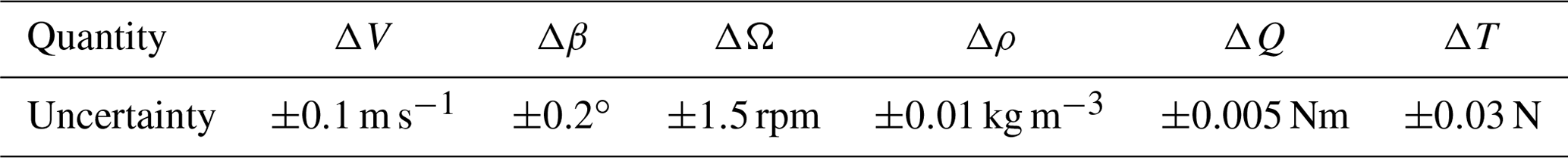
Table 1 reports a priori estimates of the uncertainties associated with the various measured quantities. Given the uncertainties of the measurements, worst-case uncertainties of the power and thrust coefficients can be readily computed as
The wind speed V was measured by a Mensor CPT-6100 pitot transducer (Mensor, 2016), which is affected by pressure and alignment errors. The pitot tube measures the dynamic pressure, i.e., the difference between the total and the static pressures. Since the wind speed is computed by inverting the dynamic pressure expression, errors in Δp and ρ directly pollute V. Additionally, a yaw and tilt misalignment may exist between the pitot axis and the incoming wind vector, increasing the error in V. The uncertainty of the air density was estimated from the hygrometer and barometer installed in the wind tunnel. After considering all relevant factors, the uncertainty of the wind speed was determined using the guidelines described in Standard ISO 3354 (2008). The uncertainty in the blade pitch angle β was estimated by calibrating the actuator encoder with a Wyler Clinotronic Plus inclinometer (Campagnolo, 2013). Power was computed as P=QΩ, where Q is the torque, which was measured by strain gages at the rotor shaft. These sensors were calibrated by applying a known torque to the locked rotor. The rotor speed Ω was measured by an optical incremental encoder with a count per revolution Ne=10 000 and an observation window tow=4 ms, which results in an error rpm. The thrust T was obtained by measuring with a strain gage bridge the fore–aft bending moment at the tower base; here again, the strain gages were calibrated by applying a known load to the turbine by a pulley-and-weight system. The contribution to the bending moment due to the drag of nacelle and rotor was obtained by a dedicated experiment in the wind tunnel without the blades. Additional details on sensors and error quantification are discussed in Campagnolo (2013) and Bottasso et al. (2014b).
For each wind speed V, a turbine should operate at a specific TSR λ and blade pitch β, which are computed in region II to maximize power capture and in region III to limit power output to the rated value. On the other hand, for the task of identifying the airfoil polars, a broad range of conditions is necessary in order to span a sufficient range of angles of attack and Reynolds of interest. Although a broad range is necessary for the generality of the identified model, the conditions that are closer to the nominal operating points – according to the regulation trajectory of the machine – are also the ones most likely encountered during the actual operation of the turbine. To account for this fact, the weight wi of each operational condition i (see Eq. 2) was assigned based on its distance to the nominal conditions, computed as
where indicates a nominal value, and are scaling factors. All data points were divided into four groups according to their distance. Data points within each group were assigned the same weight, with longer mean distances corresponding to lower weights.
4.2 Identification results
Nominal values of the blade polars are defined as the ones previously computed with the method of Bottasso et al. (2014a). Although of a good quality, these polars are not always able to correctly represent the behavior of the turbine, for example in derated conditions. To improve on this situation, the method proposed here was used to further correct the polars and provide improved estimates.
The lift and drag coefficients were parameterized in terms of bilinear shape functions using seven nodal values for Reynolds and 21 for angle of attack for each one of the two coefficients. Since the G1 blades use one single airfoil type along their entire span, it was not necessary to introduce the dependency on η appearing in the general expressions of Eq. (16).
For the nominal polars, Fig. 2 plots the variance σ2 (which is the inverse of the singular values produced by the SVD analysis) for the seven considered Reynolds numbers and the lowest 25 modes. The figure shows that modes of intermediate Reynolds number have better observability as most conditions do happen within this range. All modes with a variance above 1 (a threshold indicated in the figure by a dashed horizontal line) were discarded, reducing the number of degrees of freedom from the initial 294 to 117, which improves the well-posedness of the problem and also reduces the computational cost.
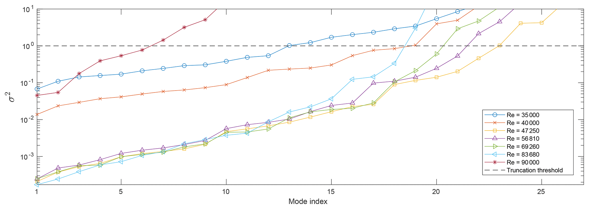
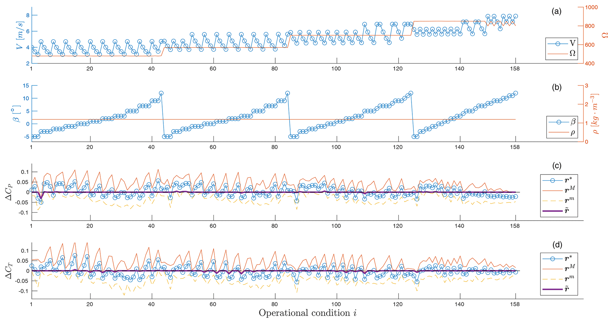
Figure 3(a, b) Nominal model inputs V, Ω, β, ρ. (c, d) Nominal, maximal, minimal, and filtered residuals for the two outputs ΔCP and ΔCT. All quantities are plotted for each one of the 158 operating conditions in the measurement set.
The identification first used nominal model inputs u* and the residual filtering technique of Sect. 2.4 to identify an initial guess to the system parameters p, a process that converged after nine major iterations of Eqs. (3) and (4). For the converged solution, Fig. 3 shows the nominal model inputs (two upper plots) and the output residuals (two lower plots), including the nominal residual r*, the maximal residual rM, the minimal residual rm, and the filtered residual (see Eqs. 13 and 14) for each one of the measured data points. The filtered residuals are 0 for most conditions, indicating that the information carried by these data points cannot be distinguished further from input measurement noise. In addition, all nonzero filtered residuals are small, indicating an almost singular , which is in fact used as a termination criterion.
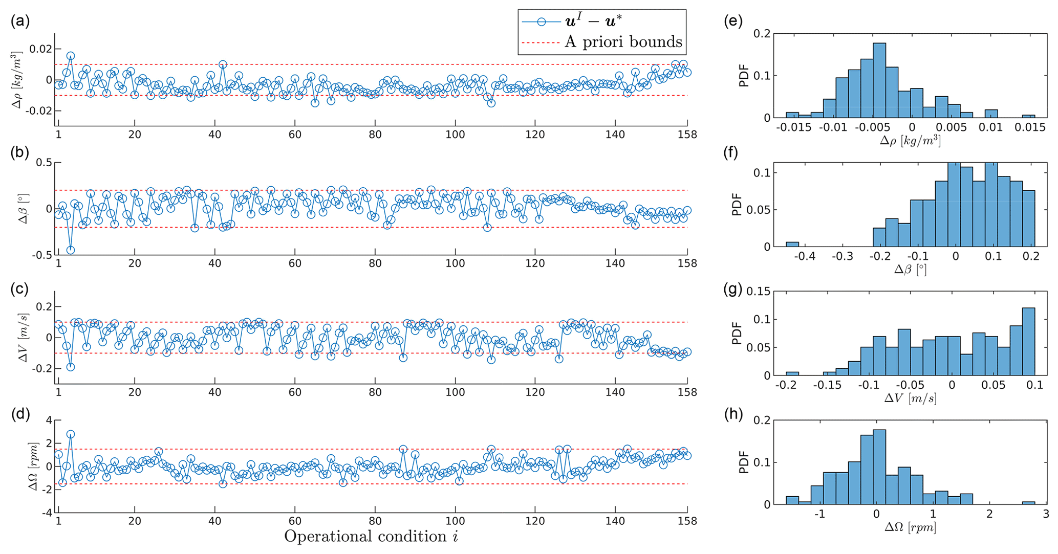
Figure 4Differences between identified and nominal inputs for all operating conditions (a–d) and their corresponding distributions (e–h).
An a priori estimate of the maximal uncertainties of the power and thrust coefficients can be computed based on Eq. (19) and Table 1, which yields
On the other hand, an a posteriori estimate of the uncertainties evaluated with nominal inputs u* is available by the covariance matrix R of Eq. (3) that, using unfiltered residuals, gives
As expected, the a posteriori estimates are smaller than the a priori ones since the latter represent a worst-case scenario.
The process was then continued using the previously converged parameters as an initial guess. Now, however, the model inputs u were added to the identification to include the effects of their uncertainties. After three iterations, a converged solution was obtained. The final identified inputs are denoted in the following as uI. For all operational conditions, Fig. 4 shows the differences between identified and nominal values. In all subplots, two dashed horizontal lines indicate the a priori uncertainties reported in Table 1. It is interesting to observe that most estimated inputs are within the a priori bounds, indicating a good coherence between a priori and a posteriori statistics. The right part of the same figure reports the distributions of the errors that, except for wind speed, are close to normal. On the other hand, density appears to have a small bias, which violates one of the assumptions of ML estimation.
Figure 5 shows the nominal (dashed lines) and identified (solid lines) lift (left plot) and drag (right plot) coefficients as functions of angle of attack for various Reynolds numbers. Values outside of the angle of attack and Reynolds ranges of the plot are not identifiable with the available data set and therefore are not shown. The nominal coefficients tuned according to Bottasso et al. (2014a) cross each other, violating the consistency constraints on the laminar separation bubble expressed by Eq. (18). In contrast, the new identified results do comply with the constraints.
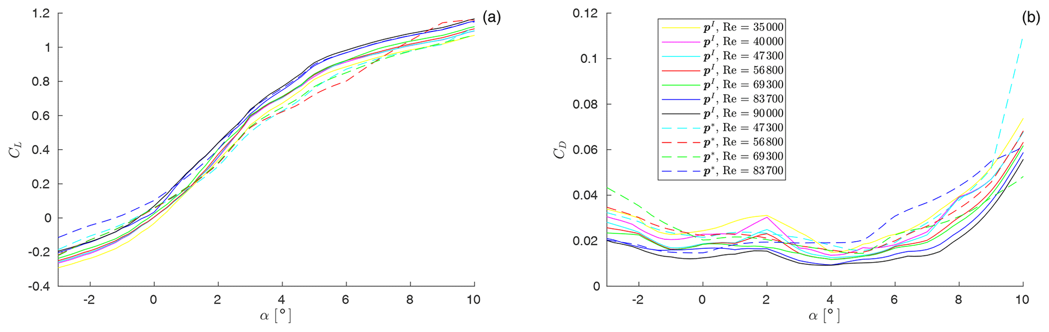
Figure 5Lift CL (a) and drag CD (b) coefficients as functions of angle of attack α for various Reynolds numbers. Dashed lines: nominal values according to Bottasso et al. (2014a); solid lines: new identified values.
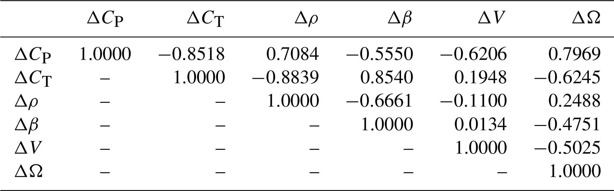
Table 2 reports the correlation coefficients, computed from the extended covariance matrix at convergence, as , where . Because of symmetry, only the upper triangle is shown.
The correlation coefficient between the two outputs, ΔCP and ΔCT, is negative. This means that, on average, at the end of the identification process the power and thrust residuals have opposite signs. This is expected since this behavior minimizes the cost function of Eq. (7). Additionally, each input induces same-sign variations in the two outputs; for example, a larger wind speed or density implies higher power and thrust coefficients, whereas a larger blade pitch implies lower power and thrust coefficients. Given that ΔCP and ΔCT have a negative correlation, the input–output correlation coefficients always have different signs for both outputs; e.g., ϱ(ΔCP, Δβ) and ϱ(ΔCT, Δβ) have opposite signs. The signs of the input–input correlations can be explained in similar terms. For example, the correlation between density and blade pitch is negative because these two inputs have correlations of opposite sign as the outputs, whereas the correlation between blade pitch and wind speed is positive because these two inputs have correlations of the same sign as the outputs.
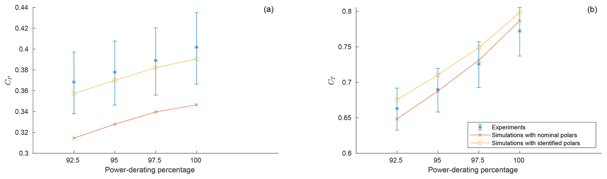
Figure 6Results for the power-derating cases. (a) Power coefficient, (b) thrust coefficient. Solid blue line with ∗ symbols: experimental results, including uncertainties according to Table 1; solid orange line with ∘ symbols: simulation results with newly identified polars; solid red lines with × symbols: simulation results with nominal polars according to Bottasso et al. (2014a).
From the extended covariance matrix at convergence, the mean absolute a posteriori uncertainties of the inputs were found to be 0.06 m s−1 for speed V, 0.09∘ for blade pitch angle β, 0.5 rpm for rotor speed Ω, and 0.005 kg m−3 for density ρ. By comparison with Table 1, all a posteriori uncertainties are smaller than the a priori ones, as expected.
4.3 Power-derating cases
To verify the quality of the identified polars, derated operational conditions were considered. It should be stressed that these conditions were not included in the identification data set and therefore provide for a verification of the generality of the results. These additional conditions are listed in Table 3 and correspond to values equal to 100 %, 97.5 %, 95 %, and 92.5 % of rated power.
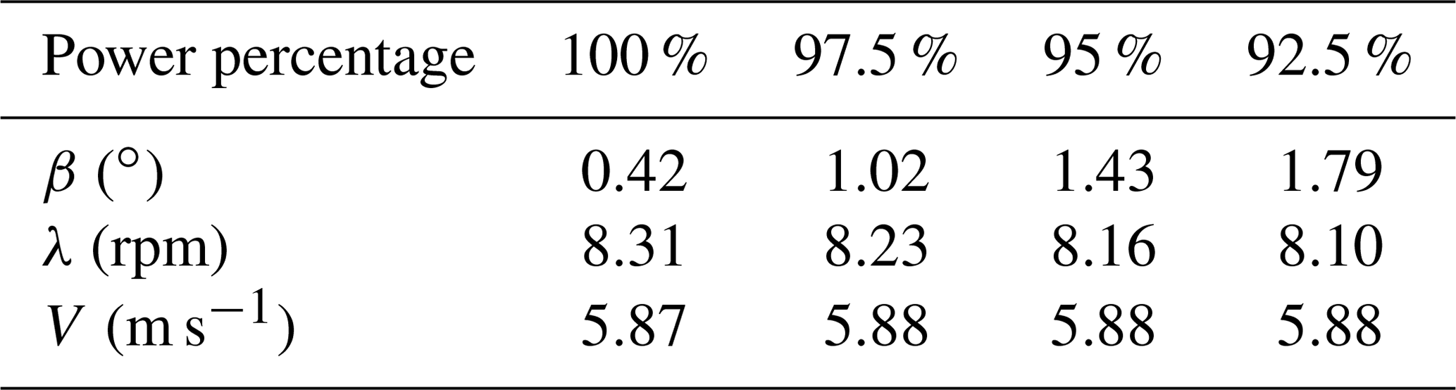
Figure 6 shows the results in terms of power (on the left) and thrust (on the right) coefficients as functions of derating percentage. In all plots, the experimental results are shown using a solid blue line with ∗ symbols; whiskers indicate the uncertainties according to Eq. (19) and Table 1. Simulation results are computed with nominal measured inputs u* for both the nominal polars p* according to Bottasso et al. (2014a) and the newly identified polars pI, and they are marked with × and ∘ symbols, respectively. The results indicate a marked improvement when using the newly identified polars, especially regarding the rotor power coefficient.
This paper has presented a new maximum likelihood identification method that, departing from the classical formulation, accounts for errors both in the outputs and the inputs. The new method is a generalization of the classical approach, where the system parameters are estimated together with the system inputs, which this way can differ from their actual measured quantities because of noise. The new expanded formulation is solved using a partitioned approach, resulting in an iteration between the standard parameter estimation and a series of decoupled and inexpensive steps to compute the inputs. To cope with the ill-posedness of the problem caused by low observability of the parameters, the formulation uses an SVD-based transformation into a new set of uncorrelated unknowns, which, after truncation to discard unobservable modes, are mapped back onto the original physical space. The formulation is further improved by an initialization step that accounts for a priori information on the errors affecting the measurements, discarding all data points whose residuals can be simply explained by uncertainties.
The new proposed formulation was applied to the estimation of the aerodynamic characteristics of the blades of small-scale wind turbine models. This is a particularly difficult problem because an extended set of parameters is necessary in order to give a meaningful description of the polars, taking into account their variability with blade span, angle of attack, and Reynolds number; invariably, this results in an ill-defined problem because of the many unknown parameters and their possible collinearity. In addition, measurement errors affect both the outputs and the inputs, the latter being particularly relevant and representing the operating conditions of the turbines. On the other hand, good-quality estimates of the polars are of crucial importance for the accuracy of simulation models based on lifting lines.
Results indicate that a higher quality of the estimates is achieved by the proposed method compared to an error-in-the-outputs-only approach. Indeed, the estimated polars were able to correctly model derated operating conditions, which were not included in the parameter estimation process. All prior attempts at modeling these conditions failed to a various extent when using the standard maximum likelihood formulation. In addition, results indicate that the present approach was able to cope with the ill-posedness of the problem caused by the low observability of the many unknown parameters, which is an important aspect for the practical applicability of the method to complex problems as the one considered in this paper.
| A | Rotor-swept area |
| CD | Drag coefficient |
| CL | Lift coefficient |
| CP | Power coefficient |
| CT | Thrust coefficient |
| J | Cost function |
| p | Pressure |
| p | Model parameters |
| P | Power |
| Q | Torque |
| r | Residual |
| R | Covariance matrix |
| Re | Reynolds number |
| T | Thrust |
| u | Model inputs |
| V | Wind speed |
| wi | Weight of the ith measurement |
| y | Model outputs |
| α | Angle of attack |
| β | Blade collective pitch angle |
| η | Nondimensional blade span location |
| λ | Tip speed ratio |
| Ω | Rotor speed |
| ρ | Density |
| ϱ | Correlation coefficient |
| σ | Standard deviation |
| Expanded quantity | |
| Filtered quantity | |
| (⋅)I | Identified quantity |
| Measured quantity | |
| ALM | Actuator line method |
| BEM | Blade element momentum |
| CFD | Computational fluid dynamics |
| FVW | Free vortex wake |
| LES | Large-eddy simulation |
| ML | Maximum likelihood |
| SVD | Singular value decomposition |
| TSR | Tip speed ratio |
An implementation of the polar identification method and the data used for the present analysis can be obtained by contacting the authors.
CW developed the a priori residual filtering method, wrote the software, performed the simulations, and analyzed the results. FC was responsible for the wind tunnel experiments and the analysis of the measurements. CLB devised the original idea of estimating polars from operational turbine data, developed the ML formulation with errors in inputs and outputs, and supervised the work. CW and CLB wrote the manuscript. All authors provided important input to this research work through discussions and feedback and by improving the manuscript.
The authors declare that they have no conflict of interest.
The authors gratefully acknowledge Stefano Cacciola of Politecnico di Milano, who provided the outputs-only version of the code. The authors also express their appreciation to the Leibniz Supercomputing Centre (LRZ) for providing access and computing time on the SuperMUC-NG system.
This work has been supported by the CL-WINDCON project, which receives funding from the European Union Horizon 2020 research and innovation program under grant agreement no. 727477.
This paper was edited by Alessandro Bianchini and reviewed by two anonymous referees.
Bottasso, C. L. and Campagnolo, F.: Wind Tunnel Testing of Wind Turbines and Farms, in: Handbook of Wind Energy Aerod., edited by: Stoevesandt, B., Schepers, G., Fuglsang, P., and Sun, Y., Springer Nature, Switzerland, https://doi.org/10.1007/978-3-030-05455-7, 2020. a, b
Bottasso, C. L., Cacciola, S., and Iriarte, X.: Calibration of wind turbine lifting line models from rotor loads, Wind Eng. Ind. Aerod., 124, 29-45, https://doi.org/10.1016/j.jweia.2013.11.003, 2014a. a, b, c, d, e, f, g, h, i, j, k, l
Bottasso, C. L., Campagnolo, F., and Petrovic, V.: Wind tunnel testing of scaled wind turbine models: Beyond aerodynamics, J. Wind Eng. Ind. Aerodyn., 127, 11–28, https://doi.org/10.1016/j.jweia.2014.01.009, 2014b. a, b, c, d
Burton, T., Jenkins, N., Sharpe, D., and Bossanyi, E.: Wind energy handbook, John Wiley & Sons, West Sussex, UK, 2011. a
Campagnolo, F.: Wind tunnel testing of scaled wind turbine models: aerodynamics and beyond, PhD thesis, Politecnico di Milano, Milano, Italy, 2013. a, b
Campagnolo, F., Petrović, V., Schreiber, J., Nanos, E. M., Croce, A., and Bottasso, C. L.: Wind tunnel testing of a closed-loop wake deflection controller for wind farm power maximization, J. Phys.: Conf. Ser., 753, 032006, https://doi.org/10.1088/1742-6596/753/3/032006, 2016. a, b
Campagnolo, F., Weber, R., Schreiber, J., and Bottasso, C. L.: Wind tunnel testing of wake steering with dynamic wind direction changes, Wind Energ. Sci., 5, 1273–1295, https://doi.org/10.5194/wes-5-1273-2020, 2020. a, b
Churchfield, M. and Lee, S.: NWTC design codes-SOWFA, NREL, available at: http://wind. nrel. gov/designcodes/simulator s/SOWFA (last access: 4 November 2020), 2012. a
Churchfield, M. J., Lee, S., Moriarty, P. J., Martinez, L. A., Leonardi, S., Vijayakumar, G., and Brasseur, J. G.: A large-eddy simulation of wind-plant aerodynamics, in: 50th AIAA, 9–12 January 2012, Nashville, Tennessee, https://doi.org/10.2514/6.2012-537, 2012. a
Fleming, P., Gebraad, P., Churchfield, M., Lee, S., Johnson, K., Michalakes, J., van Wingerden, J.-W., and Moriarty, P.: SOWFA Super-controller User's Manual, National Renewable Energy Laboratory, Golden, Colorado, USA, 2013. a
Frederik, J. A., Weber, R., Cacciola, S., Campagnolo, F., Croce, A., Bottasso, C., and van Wingerden, J.-W.: Periodic dynamic induction control of wind farms: proving the potential in simulations and wind tunnel experiments, Wind Energ. Sci., 5, 245–257, https://doi.org/10.5194/wes-5-245-2020, 2020. a, b
Gebraad, P., Teeuwisse, F., Wingerden, J., Fleming, P. A., Ruben, S., Marden, J., and Pao, L.: Wind plant power optimization through yaw control using a parametric model for wake effects – a CFD simulation study, Wind Energy, 19, 95–114, 2016. a
Jategaonkar, R. V.: Flight vehicle system identification: a time-domain methodology, American Institute of Aeronautics and Astronautics, Reston, VA, USA, 2015. a, b, c, d
Klein, V. and Morelli, E. A.: Aircraft system identification: theory and practice, American Institute of Aeronautics and Astronautics, Reston, VA, USA, 2006. a, b, c
Lyon, C. and Selig, M. S.: Summary of low speed airfoil data, SOARTECH Publications, Virginia Beach, VA, USA, 1997. a, b
Manwell, J. F., McGowan, J. G. and Rogers, A. L.: Wind energy explained: theory, design and application, John Wiley & Sons, Hoboken, NJ, USA, 2010. a, b
Mensor: Precision Pressure Transducer Models CPT6100, CPT6180, WIKA Alexander Wiegand SE & Co. KG, Klingenberg, Germany, available at: http://www.wika.rs/upload/DS_CT2510_en_co_34182.pdf (last access: 4 November 2020), 2016. a
OpenFast: OpenFast documentation – Release v2.3.0, National Renewable Energy Laboratory, Golden, Colorado, USA, 2 April 2020. a, b
Sebastian, T. and Lackner, M. A.: Development of a free vortex wake method code for offshore floating wind turbines, Renew. Energy, 46, 269–275, https://doi.org/10.1016/j.renene.2012.03.033, 2012. a
Selig, M. S. and McGranahan, B. D.: Wind tunnel aerodynamic tests of six airfoils for use on small wind turbines, J. Sol. Energ. Eng., 126, 986–1001, https://doi.org/10.1115/1.1793208, 2004. a
Shaler, K., Kecskemety, K. M., and McNamara, J. J.: Benchmarking of a free vortex wake model for prediction of wake interactions, Renew. Energy, 136, 607–620, https://doi.org/10.1016/j.renene.2018.12.044, 2019. a
Standard ISO 3354: Measurement of clean water flow in closed conduits–Velocity-area method using current-meters in full conduits and under regular flow conditions, Inter. Org. for Standardization, UK, 2008. a
Troldborg, N., Sørensen, J. N., and Mikkelsen, R.: Actuator line simulation of wake of wind turbine operating in turbulent inflow, J. Phys.: Conf. Ser., 75, 012063, https://doi.org/10.1088/1742-6596/75/1/012063, 2007. a
Wang, J., Wang, C., Campagnolo, F., and Bottasso, C. L.: Wake behavior and control: comparison of LES simulations and wind tunnel measurements, Wind Energ. Sci., 4, 71–88, https://doi.org/10.5194/wes-4-71-2019, 2019. a, b, c, d
Wang, C., Muñóz-Simon, A., Deskos, G., Laizet, S., Palacios, R., Campagnolo, F., and Bottasso, C. L.: Code-to-code-to-experiment validation of LES-ALM wind farm simulators, J. Phys.: Conf. Ser., 1618, 062041, https://doi.org/10.1088/1742-6596/1618/6/062041, 2020a. a
Wang, C., Campagnolo, F., Sharma, A., and Bottasso, C. L.: Effects of dynamic induction control on power and loads, by LES-ALM simulations and wind tunnel experiments, J. Phys.: Conf. Ser., 1618, 022036, https://doi.org/10.1088/1742-6596/1618/2/022036, 2020b. a
Wang, C., Campagnolo, F., and Bottasso, C. L.: Does the use of load-reducing IPC on a wake-steering turbine affect wake behavior, J. Phys.: Conf. Ser., 1618, 022035, https://doi.org/10.1088/1742-6596/1618/2/022035, 2020c. a