the Creative Commons Attribution 4.0 License.
the Creative Commons Attribution 4.0 License.
 | 26 Nov 2020
Mitigation of offshore wind power intermittency by interconnection of production sites
Ida Marie Solbrekke
Nils Gunnar Kvamstø
Asgeir Sorteberg
This study uses a unique set of hourly wind speed data observed over a period of 16 years to quantify the potential of collective offshore wind power production. We address the well-known intermittency problem of wind power for five locations along the Norwegian continental shelf. Mitigation of wind power intermittency is investigated using a hypothetical electricity grid. The degree of mitigation is examined by connecting different configurations of the sites. Along with the wind power smoothing effect, we explore the risk probability of the occurrence and duration of wind power shutdown due to too low or high winds. Typical large-scale atmospheric situations resulting in long term shutdown periods are identified. We find that both the wind power variability and the risk of not producing any wind power decrease significantly with an increasing array of connected sites. The risk of no wind power production for a given hour is reduced from the interval 8.0 %–11.2 % for a single site to under 4 % for two sites. Increasing the array size further reduces the risk, but to a lesser extent. The average atmospheric weather pattern resulting in wind speed that is too low (too high) to produce wind power is associated with a high-pressure (low-pressure) system near the production sites.
- Article
(2553 KB) - Full-text XML
- BibTeX
- EndNote


Renewable power generation from various sources is continuously increasing. This is a desired development due to, among others things, emission goals that are linked to mitigation of global warming. Offshore wind power, and especially floating offshore wind power, is only in an initial phase compared to other more mature and developed energy sources. A study by Bosch et al. (2018) has found the global offshore wind energy potential to be 329.6 TWh, with over 50 % of this potential being in deep waters (>60 m). These numbers underline the need to take advantage of the floating offshore wind energy source with a view to addressing the continuous growth in global energy consumption.
Exploiting the offshore wind energy potential introduces a number of challenges, one of which is the variable nature of the energy source. The wind varies on both spatial and temporal scales, ranging from small features existing for a few seconds to large and slowly evolving climatological patterns. This intermittency results in a considerable variability on different time and spatial scales, leading to highly fluctuating power production and even power discontinuities of various durations.
Fluctuating wind power production is shown to be dampened by connecting dispersed wind power generation sites (Archer and Jacobson, 2007; Dvorak et al., 2012; Grams et al., 2017; Kempton et al., 2010; Reichenberg et al., 2014, 2017; St. Martin et al., 2015). This smoothing effect was demonstrated as early as 1979 by Kahn (1979), who evaluated the reliability of geographically distributed wind generators in a California case study. As weather patterns are heterogeneous, the idea behind connecting wind farms that are situated far apart is that the various sites will experience different weather at a certain time. There is therefore potential to reduce wind power variability as wind farms, unlike single locations, are area-aggregated.
Previous studies examine this smoothing effect almost exclusively over land (Archer and Jacobson, 2007; Grams et al., 2017; Kahn, 1979; Reichenberg et al., 2014, 2017; St. Martin et al., 2015). For example, Reichenberg et al. (2014) presented a method to minimize wind power variability using sequential optimization of site location applied to the Nordic countries and Germany. They found that by using optimal aggregation the coefficient of variability CV () was reduced from 0.91 to 0.54, meaning that wind power variability was substantially reduced when utilizing the fact that the connected production sites were located far apart and in different wind regimes. In addition to intermittency reduction, combining a number of wind power sites situated throughout Europe has also resulted in a reduced number of low-power events. Reichenberg et al. (2017) focused on minimizing the variables related to wind power variability and maximizing the average wind power output and found that periods of low output were almost completely avoided.
A few studies have examined the smoothing effect of production sites distributed over the ocean (Dvorak et al., 2012; Kempton et al., 2010). Kempton et al. (2010) studied the stabilization of the wind power output by placing the production sites in an optimal meteorological configuration and connecting them. They used data from 11 (more or less) meridionally oriented meteorological stations spanning 2500 km along the east coast of the US. They concluded that connecting all 11 sites resulted in a slowly changing wind power output, in addition to a production that rarely reached either full or zero wind power output. Dvorak et al. (2012) also used the east coast of the US as a study area, but at shallow water depths (≤50 m), in an attempt to identify an ideal offshore wind energy grid in terms of, among other things, a smoothed wind energy output and a reduced hourly ramp rate and hours of zero power. They found that by connecting all four farms included in the study the power output was smoothed and the hourly zero-power events were reduced from 9 % to 4 %. They also found that wind power production in regions driven by both synoptic-scale storms and mesoscale sea breeze events experienced a substantial reduction in low- or zero-production hours and in the amplitude of the hourly ramp rates when all four farms were connected, compared to production from single farms.
This study is based on 16 years of wind observations from a unique string of sites along the Norwegian coast. We analyze the potential intermittency reduction of wind power output over open ocean by potentially connecting up to five power-producing sites in different combinations. The water depth at these locations ranges from 75 m at Ekofisk to over 350 m at Norne, which means that floating offshore wind is more or less the only option. We approximate the wind power output by transforming hourly observed wind speed observations to wind power output through a conversion function. Along with the smoothing effect, we also investigate statistical wind power characteristics as a function of production site combinations. Additionally, we quantify the potential reduction in the occurrence and duration of shutdown events (no production of wind power).
Identifying typical atmospheric weather conditions that often result in long-term zero wind power production is crucial. During these shutdown events the power demand has to be covered by other energy sources or through energy storage systems such as hydrogen or batteries. It is therefore important to map and identify these critical weather patterns, particularly if wind is likely to constitute a large share of the global energy and electricity mix. Kempton et al. (2010) examined a few high- and low-power events using reanalysis data to gain insight into the corresponding large-scale atmospheric situation. In contrast to Kempton's work, we have, by examining the composition of the atmospheric situations related to zero events, revealed the typical (composite mean) atmospheric condition related to zero events caused by “too low” and “too high” wind speed.
The paper is structured as follows: Sect. 2 includes the data and the corresponding post-processing, Sect. 3 describes the methods used, and Sect. 4 presents the results of the study and discusses the results. Finally, Sect. 5 summarizes the main results in bullet points.
In this study we examine the effect of collective wind power at five locations (oil and gas platforms) along the coast of southern Norway. The data sites included in this study are Ekofisk (ek), Sleipner (sl), Gullfaks C (gf), Draugen (dr), and Norne (no) (see Fig. 1 for location and Table 1 for further information on the various sites).
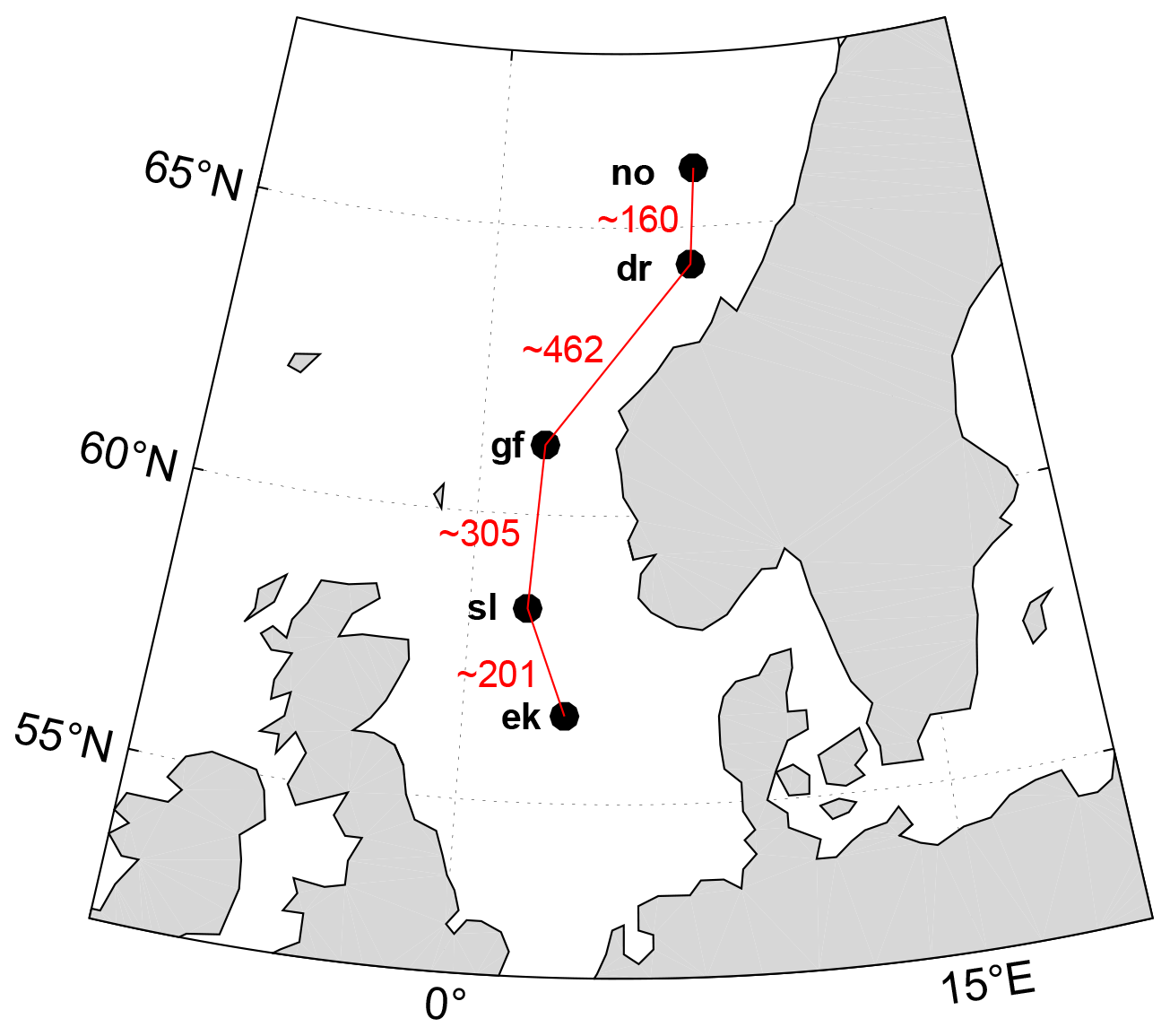
Figure 1Position of the five sites and the distance (km) between them (red lines). Abbreviations are as follows. ek: Ekofisk; sl: Sleipner; gf: Gullfaks C; dr: Draugen; no: Norne.
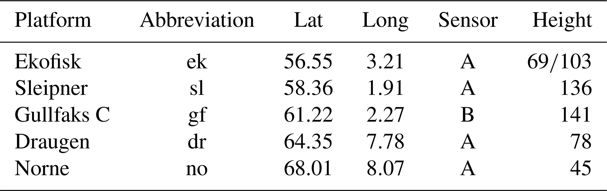
Table 1Name, abbreviation, and location (in latitude and longitude) of each site, as well as the height (m a.s.l.) of the chosen wind sensor (A or B), giving the representative wind speed time series for each site. The chosen sensor at Ekofisk (ek) has two heights since the sensor was moved during the period 2000–2016.
The observed data constitute a unique data set retrieved from the Norwegian Meteorological Institute, and the time series covers the 16-year period between 2000 and 2016. We use hourly 10 min average values1. The observed data at each site underwent a quality check, both automatic and visual. Some of the values in the data sets were recorded as NaN (not a number). In addition, some observed wind speed values were regarded as nonphysical and replaced with NaN in the time series prior to the analysis. If the data point fell into one of the three categories below, it was flagged and replaced by NaN:
-
observations with a wind speed tendency m s−2 over each of 2 consecutive hours – a spike in the wind speed time series;
-
observations dropping to zero from u≥5 m s−1 in 1 h;
-
observations of u=0 surrounded by NaN.
At each platform two anemometers were mounted at different heights, measuring the wind speed and direction. The two anemometers record two separate time series, and one of the data sets was selected to represent the wind conditions at the site in question. When choosing the most representative wind speed time series, the data set had to fulfill certain criteria, namely
-
containing the most valid observations after the flagging procedure above and
-
having the highest correlation with NORA10 reanalysis data, i.e., nearest grid point with wind speed at 100 m. (Reistad et al., 2011).
As an approximation, we can estimate the wind speed at a height level z2 by extrapolation of the wind speed from height z1 by the following relation:
where and are the wind speed at heights z2 and z1, respectively. α is the power-law exponent modifying the shape and steepness of the vertical wind speed profile, depending on both the surface roughness and the atmospheric stability (Emeis, 2018). In our study z2 is the hub height of 100 m a.s.l. and z1 is the height of the wind sensors and α=0.12. This way we obtain the extrapolated wind speeds at the hub height for each site. This power law is used and discussed by Barstad et al. (2012), among others.
After replacement of the physically unrealistic observations with NaN, and the aforementioned height extrapolation and correlation check with the NORA10, we selected the wind speed data set assumed to be the most representative for the site in question. In the following sections all estimates involve only wind speed, since we assume that turbine technology allows utilization of wind power to be independent of wind direction. Moreover, we performed calculations for one turbine at each site, since we assumed that the park effect was not relevant for the results obtained.
3.1 Estimation of wind power
The maximum part of the kinetic wind energy per time unit passing the area spanned by a wind turbine that can be utilized is defined as the wind power, P (see e.g., Jaffe and Taylor, 2019) and is written as
where β is the Betz limit, ρ is the density of the air, A is the swept area of the rotors, and u is the wind speed.
An analysis of the actual or theoretical wind power potential would involve an analysis of the time series of P. However, a more practical approach is needed as current technology only allows turbines to produce power at certain wind speed intervals. Power production starts when the wind exceeds a “cut-in” value uci. Subsequently, total wind power production, , increases according to until u reaches the rated wind speed value ur. The rated wind speed denotes the transition limit where the turbine starts to produce at rated power. For higher wind speeds, u>ur, is kept constant until u reaches a “cut-out” value, uco. Thereafter the production is terminated () abruptly with increasing wind. This abrupt termination of wind energy due to too high winds is a storm shutdown and is called “storm control”. In practice, the described production regime for u>ur is brought about by instantaneous pitching of turbine blades. This pitching allows a portion of the energy to pass through the blades without utilization and is done to shelter the turbines from the harsh drag force and to minimize the turbines' maintenance. Consequently, the maximum power outtake for a turbine occurs when and can be written as . In practice, is the installed capacity. In order for our results to be as general as possible in the rest of the paper, and since the turbine park at each site is only imaginary and of unknown capacity, we normalize the power calculations . The technological characteristics of the turbines thus result in a transformation P→Pw, which can be written as
where u is the wind speed data, uci=4 m s−1 is the cut-in wind speed, ur=13 m s−1 is the rated wind speed, and uco=25 m −1 is the cut-out wind speed. These numbers are retrieved from the SWT-6.0-154 turbines used in Hywind, Scotland (Siemens AG, 2011). The SWT-6.0-154 turbines were selected as they are the turbines used in the world's first commercially operating floating wind farm off the coast of Scotland.
4.1 Wind speed and wind power characteristics
Some statistical quantities are studied to reveal both wind speed and wind power characteristics: for the wind speed the Weibull mean (μ) and standard deviation (σ), together with the scale and shape parameters (a and b), are calculated (see upper panel of Fig. 2 for an example wind speed distribution).
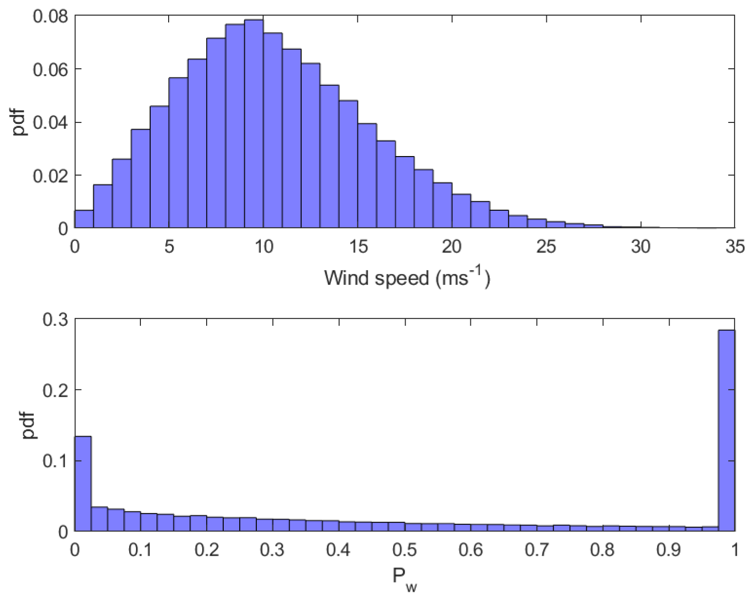
Figure 2Example distribution for Ekofisk (ek) showing the probability density function (pdf) for both wind speed (m s−1) and normalized wind power (Pw).
After conversion of wind speed to wind power via Eq. (3), the data obtain an entirely different distribution (see lower panel of Fig. 2 for an example of wind power distribution). Calculating the arithmetic mean and standard deviation will most likely not result in values representing the typical wind power output and the associated variability. Instead, we use the median (q2) and interquartile range (IQR) as a measure of the middle value and the spread in the data, respectively. Both q2 and IQR are independent of the data distribution, which makes them adequate choices to represent the statistical characteristics of the wind power data.
Table 2Statistical measures of the wind speed and wind power. μ and σ are the Weibull mean and standard deviation, respectively, a and b are the scale and shape parameter of a Weibull distribution, respectively, q50 is the median (second quartile), IQR is the interquartile range, RCoV is the robust coefficient of variability, and CF is the wind power capacity factor.
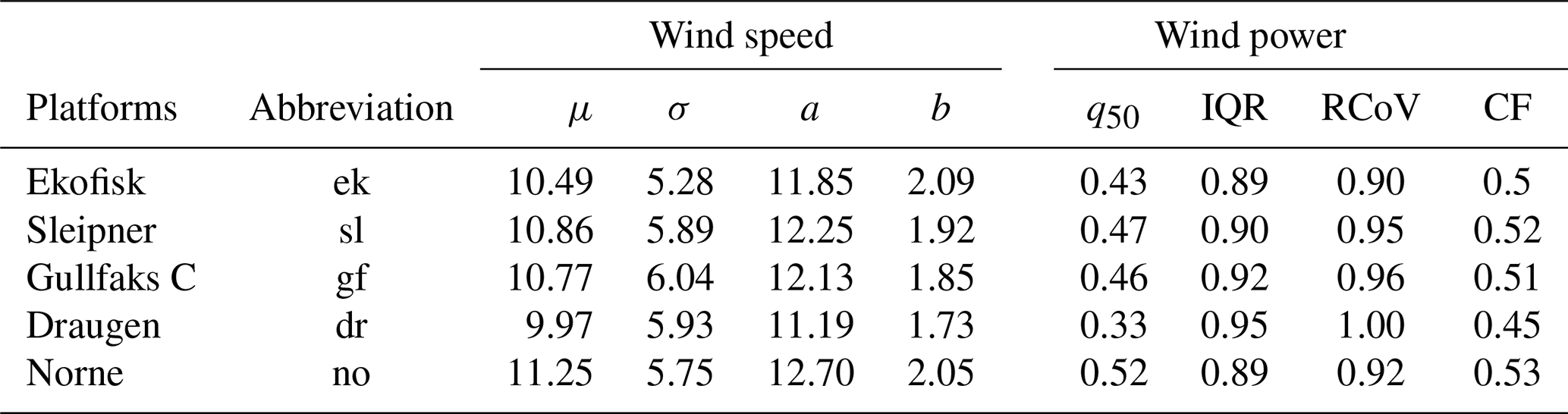
The mean wind speed values (μ) for the five sites demonstrate that the potential for wind power harvest is very good, with the mean ranging from 9.97 to 11.25 m s−1. Zheng et al. (2016) regarded the wind speed at 90 m a.s.l. in the Norwegian Sea and the North Sea as “superb” and ranked it in the highest wind category (category 7) with the potential to produce more than 400 W m−2 of wind energy. By comparison, many of the wind parks already operating in the Yellow Sea (east of China) are only ranked in categories 4–6, ranging from “good” to “outstanding”, with the potential to produce 200–400 W m−2, respectively.
As mentioned earlier, the wind power intermittency is a huge problem due to the balancing difficulties and high economic costs related to a fluctuating power output. Among the five platforms, Ekofisk (ek) has the lowest variability, with a standard deviation of 5.3 m s−1. Gullfaks C (gf) is the site with the highest variability, where σ=6.0 m s−1. a is the scale parameter giving the height and width of the Weibull distribution. A large (small) scale parameter indicates a wide and low (high and narrow) distribution. For this data set a ranges from 11.2 to 12.7 for Draugen (dr) and Sleipner (sl), respectively. b tells us about the shape of the distribution. A small b (b<3) means that the distribution is positively skewed, with a long tail to the right of the mean. The smaller the number, the more right-skewed the distribution. Here, b ranges from 1.73 to 2.09 for Draugen (dr) and Ekofisk (ek), respectively, meaning that all the distributions are positively skewed, confirming that the wind speed has more of a Weibull distribution than a Gaussian distribution. Since the goal of a functioning wind park is to produce as much wind power as possible, it is desirable that the wind speed data fall between 4 m s m s−1, or even more preferably between 13 m s m s−1 which will give Pw=1. Sleipner (sl) is the site that most frequently operates at rated power: slightly over 30 % of the time. This is a result of the fact that Sleipner (sl) has an optimal combination of the scale (12.3) and shape (1.9) parameter, with the largest portion of the wind speed distribution falling between 4 and 25 m s−1.
For the wind power, the median values (q50) range from 0.33 for Draugen (dr) to 0.52 for Norne (no). Another measure of the performance of a wind park is the capacity factor (CF), which is defined as the annual mean power production divided by the installed capacity. Draugen (dr) has the lowest capacity factor, CF=0.45, and Norne (no) has the highest, with CF=0.53. The wind power IQR is high, around 0.9. This means that contains 50 % of the wind power output. There is therefore potential for reducing wind power intermittency by combining sites.
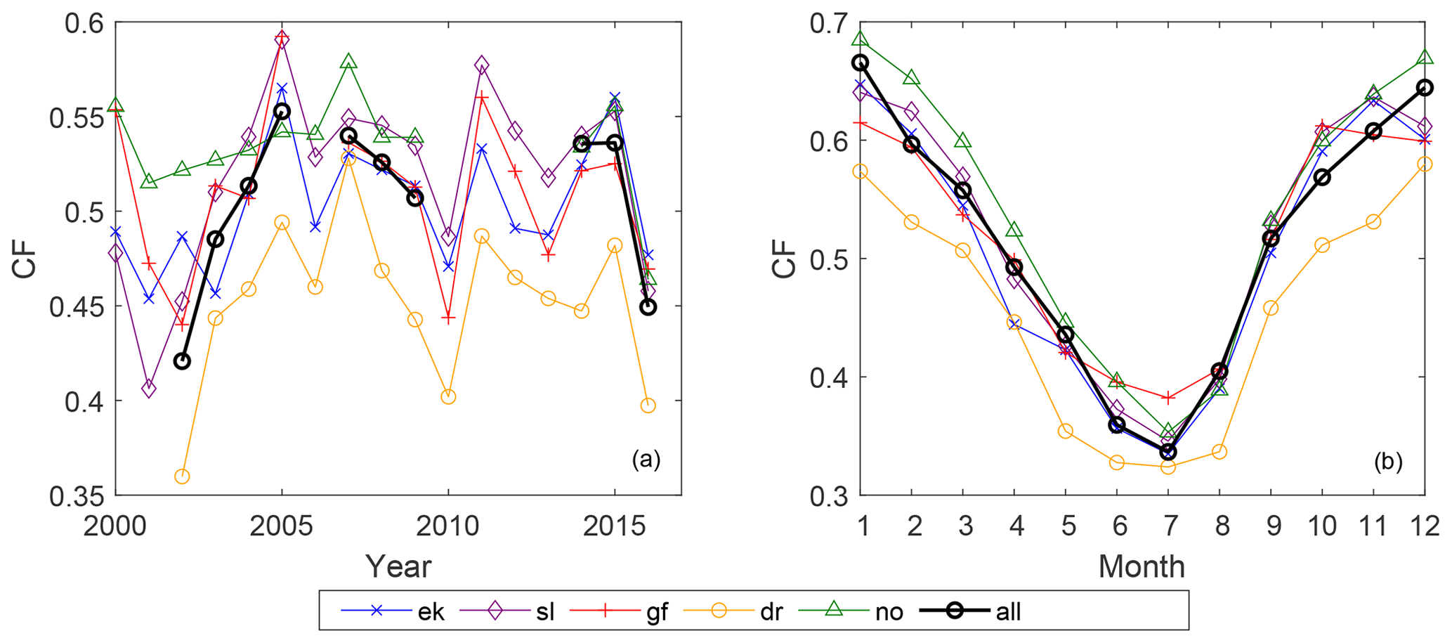
Figure 3(a) Interannual variation in the capacity factor (CF) for the five sites and the total interconnected system (“all”). If more than half of the data in 1 year were missing, the value for that year was excluded in the plot. (b) The seasonal variation in CF for the five sites and the interconnected system (“all”).
Reichenberg et al. (2014) concluded that the coefficient of variability for wind power can be substantially reduced by geographic allocation of the production sites. They used the arithmetic mean (μ) and standard deviation (σ), calculating the coefficient of variability (). As mentioned above, using the arithmetic mean and standard deviation gives rise to a misleading interpretation of the actual middle value and the accompanying variability of the wind power output. This is due to the very different wind power distribution arising from the nonlinear conversion of the wind speed data to wind power output through the power conversion curve (see Eq. 3). Hence, another more robust and resistant measure of wind power variability is the RCoV (Lee et al., 2018). The is the median absolute deviation (MAD) divided by the median (q50) and is a normalized measure of the spread in the data set. Here, RCoV ranges from 0.9 for Ekofisk (ek) to 1.00 for Draugen (dr), meaning that a typical deviation from the median value is approximately equal to the median value itself.
4.1.1 Interannual and seasonal wind power variability
How CF varies from one year to another gives a good indication of the long-term fluctuations in wind power production. The annual variation in CF can be quite substantial and is presented in Fig. 3a. For all the sites, the interannual variation can change by up to 0.12 (12 % of installed capacity) from one year to the next (i.e., 2010–2011). On this timescale, the CF values for the five stations follow each other more or less, bearing in mind that on an annual timescale, the production in the whole region will strongly co-vary. The strong interannual variations in CF clearly demonstrate that measuring the wind conditions over too short of a time period (i.e., 1 year) is generally not sufficient to estimate a representative wind power potential for a site at these latitudes.
Figure 3b presents the seasonal variation in CF. The highest CF values are found during the autumn and winter (October–February) and range from 0.58 to 0.68 for the northernmost sites Draugen (dr) and Norne (no), respectively. The lowest CF values occur during the summer and range from 0.32 at Draugen (dr) to 0.38 at Gullfaks C (gf).
4.2 Correlation and intermittency
In terms of reducing wind power variability, the optimal hypothetical case would have been to combine production from two stations with correlation coefficient . The two combined sites would then be completely out of phase, and the sum of the individual productions would be constant in time, given equally installed capacity at each site. Since the synoptic weather systems constitute the main source of spatiotemporal variance in wind over open ocean, the connected production sites situated far apart in our site array will probably experience the most contrasting weather and therefore result in the largest dampening of the wind power intermittency. To quantify this, we investigated the pairwise correlation between the different wind power time series (Pw) as a function of distance and time lag between the hypothetically connected sites. Sinden (2007) analyzed the characteristics of the wind power resource for 66 onshore sites in the United Kingdom. He found a substantial reduction in the correlation between site pairs at separation distances less than 600 km. However, for wind sites located more than 800 km apart, the decrease in correlation is less pronounced, despite a further increase in the distance between them. Our results confirm this distance dependency of the correlation found in Sinden (2007): Fig. 4 illustrates how the correlation between station pairs changes as a function of the separation distance. The correlation drops off quickly as the distance (x) between the sites increases. After x≈800 km the decrease in correlation with distance is reduced to 0.1 and continues to decrease more slowly with increasing separation distance. It is expected that the correlation between site pairs will approach zero when the separation distance becomes large enough, meaning that the wind at these sites is completely independent. Some site pairs can even have slightly negative correlation. Reaching this slowdown in the relation between the correlation and the separation distance after x≈800 km indicates that combining sites outside a radius of x≈800 km for further variability reduction has almost a negligible effect for the length and timescales considered here. Nevertheless, the correlation coefficient never drops to zero, or below zero, over the range of the data covered in this study, indicating that none of these station pairs will either be anticorrelated or have completely independent production (r≤0).
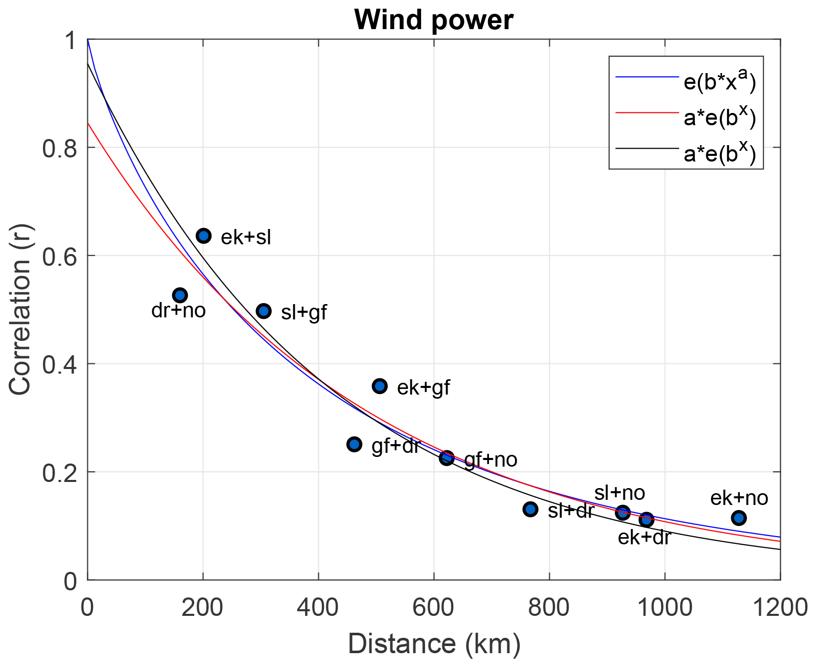
Figure 4How the correlation between site pairs changes with distance, including three exponential curves giving the best least-squares fit for the 10 correlation points.
The decorrelation length illustrates at what radius the wind power correlation drops to a fraction of the initial value at x=0. In our study, we use the e-folding distance2 as a measure of the decorrelation length L. The 10 station pairs are used to identify a best-fitting curve describing the dependency between correlation and separation distance, which will give a general description of the decorrelation length L (in kilometers). Identifying such a best-fitting curve may be challenging, and we therefore use three exponential functions with slightly different properties to indicate the uncertainty in the estimates due to the choice of fitting function. The exponential curves, together with the 10 correlation points are presented in Fig. 4, while the corresponding decorrelation lengths are presented in Table 3. The decorrelation length L is slightly more than 400 km. St. Martin et al. (2015) identify decorrelation lengths in the same order using the e-folding distance (L=388, L=685, and L=323 km for three different regions: southeastern Australia, Canada, and the northwestern US, respectively). Further, they argue that more correct decorrelation lengths can be obtained by using the e-folding distance times the nugget effect (βL) and even better results by using the integral-scale matrix ξτ. The integral-scale matrix is a measure of the distance required for the correlation to fall to a small value compared to unity. Both measures mentioned above gave a decorrelation length substantially less than the e-folding distance with βL=273, 447, 130 km and ξτ=273, 368, 89 km. St. Martin et al. (2015) also concluded that the decorrelation length is highly sensitive to the variability timescale. This result is also obtained in this study (not shown) and in Czisch and Ernst (2001). On timescales longer than a day, St. Martin et al. (2015) found that the benefit of variability reduction from aggregation of wind power over a region of a given size is independent of timescale. Therefore, if two of our offshore wind-producing sites were to balance each other at short timescales (<1 h), the separation distance could be further reduced from L=400 km. On the other hand, if they were to balance each other on longer timescales (>1 h), the separation distance would be larger than L=400 km. This is a significant result because it underlines the importance of considering timescales when combining wind-power-producing sites to reduce wind power intermittency.
Table 3Annual and seasonal decorrelation length L (in kilometers) for the three exponential functions in Fig. 4. The third column represents a fit where the point [x, y]=[0, 1] is added to the data points to include that the correlation = 1 when the x=0.

In general, the seasonal L is shorter than the annual decorrelation length (see Table 3). The winter months (December–February) contain the shortest decorrelation lengths, varying from L=289 to 301 km, depending on the exponential fit. During the winter, the atmosphere is more irregular and chaotic in both space and time, meaning that two stations located a given distance apart will more often enter different wind regimes during the winter than the other seasons. The summer months (June–August) have the longest decorrelation lengths, spanning from L=388 to 395 km. The large-scale atmospheric patterns are larger, smoother, more stationary, and last longer. As demonstrated by St. Martin et al. (2015), among others, the decorrelation length is sensitive to the variability timescale. The decorrelation length increases when the variability timescale increases. When looking at variability on an annual timescale, the seasonal variability also has to be balanced. Hence, the annual decorrelation length is larger than the seasonal decorrelation length.
Figure 5 demonstrates how the time lag of maximum correlation between station pairs changes with distance. In accordance with our expectations, the sites that are closest to each other have the shortest time lag and the highest correlation, implying shorter time for the feature to propagate between them, resulting in a higher correlation. The high-pressure and especially the low-pressure systems that sweep over the North Sea and the Norwegian Sea have a prevailing traveling direction from west to east, due to the strong westerlies at these latitudes. This implies that winds accompanying the system will strike the westernmost site, Sleipner (sl), first, followed by Ekofisk (ek) and Gullfaks (gf) C at short time intervals, and later Draugen (dr) and Norne (no). A large time lag is beneficial for wind energy production. Then, a wind event will not occur simultaneously at both the connected sites. To ensure a time lag approaching 10 h, from one site experiencing a certain wind event to the other connected site experiencing the same wind event, the separation distance needs to exceed ≈600 km.
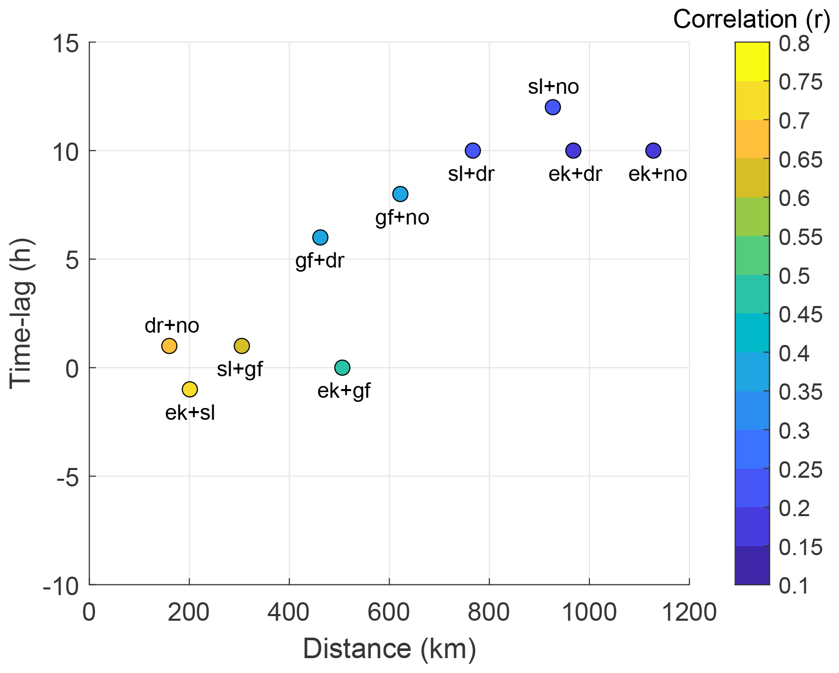
Figure 5Time lag (h) of maximum correlation between the connected sites as a function of the distance between them.
4.3 Connecting wind power sites
To study the effect of interconnected production sites, we have to make combined wind power time series for all the different site configurations. The collective wind power time series, , for different configurations of sites are found by calculating the average power production for each time step. Time steps containing NaN values for any of the sites in the configuration in question are not included. Hence, for a given time step,
where i=1, 2, …, N is the time step, j=1, 2, …, J is the number of sites combined, and is the different wind power time series for an array combination of j sites (one to five sites) at time step i.
For example, a combination of two sites (a and b) at time step i will be
This calculation is done for each time step i, as long as or .
As mentioned in Sect. 4.1 the IQR is a candidate for estimating wind power variability (Kempton et al., 2010). According to Lee et al. (2018) a more robust and resistant variability measure is the robust coefficient of variability (RCoV). Figure 6 presents IQR and RCoV for different configurations of collective wind power production, . Common to both the variability measures is that the variability generally decreases quickly with increasing array size of connected sites. This result clearly demonstrates the advantage of having interconnected wind power production in terms of intermittency reduction: Instead of operating wind turbines at two sites separately, we see that the intermittency of a connected site pair is reduced and is further reduced with increased array size. The site with the highest (lowest) IQR is the station with the lowest (highest) RCoV, since RCoV is normalized by the median value.
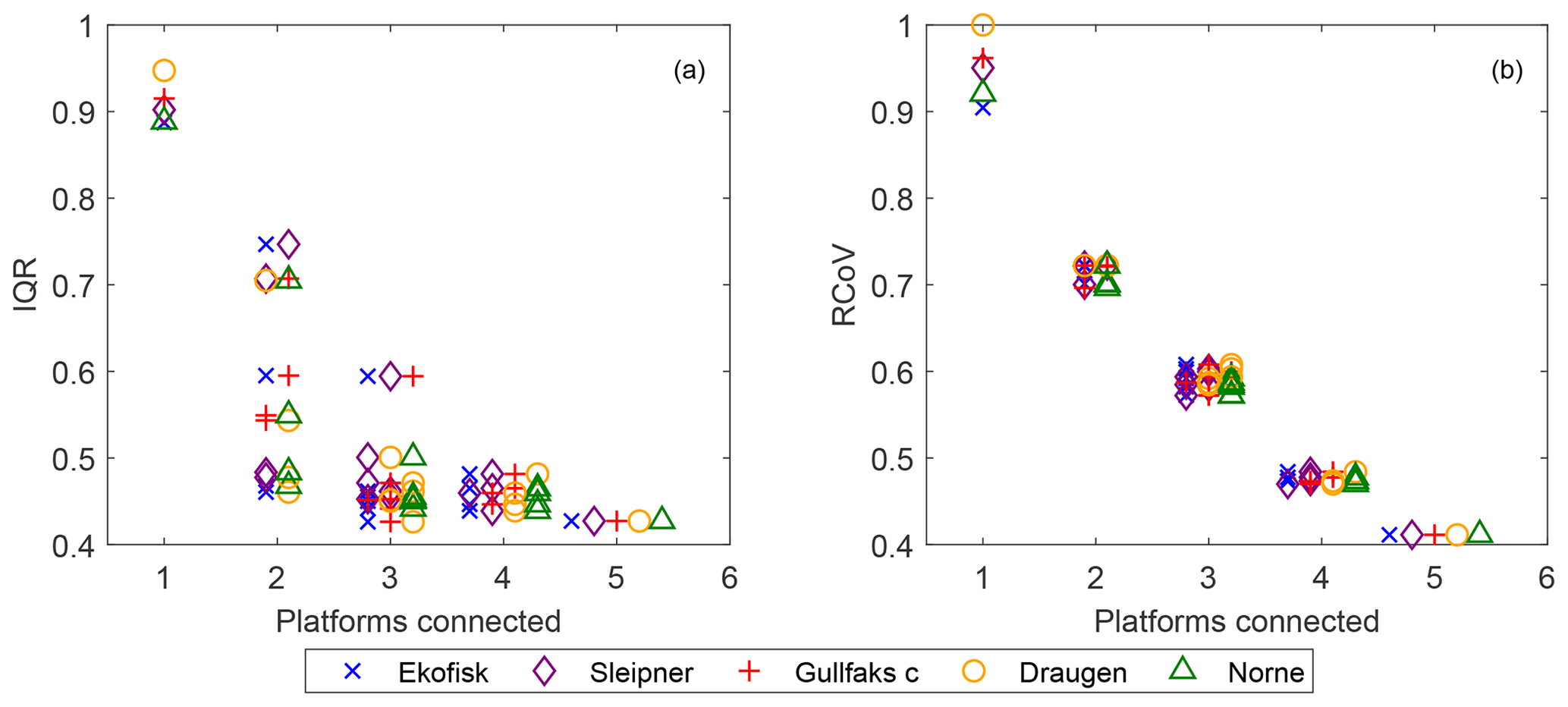
Figure 6Panels (a) and (b) demonstrate how IQR (interquartile range) and RCoV (robust coefficient of variability) change as the array size of connected sites increases from one (single sites) to five (all sites connected), respectively.
A counterintuitive result is that for some site combinations the variability (IQR and RCoV) is less than the variability for a larger array size. For example, the combination of ek + sl + gf has a higher variability than most of the pairwise site combinations. Some pairwise combinations even have a lower IQR and RCoV than a four-site combination. This result appears to be a consequence of the geographic locations of the sites in this study. Since Ekofisk (ek), Sleipner (sl), and Gullfaks C (gf) are roughly aligned in a north–south direction, they will experience the same wind event more or less simultaneously (see Fig. 5) due to the passage of extratropical cyclones and the associated fronts. Therefore, a combination of these sites would be poorer in terms of intermittency reduction than other site combinations, and even combinations of smaller array size.
4.3.1 Wind power generation duration
A typical wind power distribution can be seen in Fig. 2 (lower panel). When connecting sites, the wind power distribution changes shape. As the array size of interconnected sites increases, the distribution converges towards a bell-shaped distribution (Kempton et al., 2010). Unlike the individual distributions, where the most frequent wind power production is Pw=1 followed by Pw=0, the interconnection of production sites results in a production capacity that more regularly falls in the middle of the production range ([0 1]). Nevertheless, it is worth mentioning that when all five sites are combined, the most frequent production mode is still , indicating that full production is still the most common production state. This result arises since the five sites are located in a superb wind speed climate. This result can be further discussed in conjunction with the generation duration curve (GDC). Here, the GDC is given as a percentage of the total time the wind power output is above or below a given threshold. As can be seen in Fig. 7, the individual sites produce no power at all between 8 % and 12 % of the time. This is in contrast to the interconnected system (“all”) that almost never experiences zero wind power production. The less steep curve from the interconnected system indicates a less fluctuating output, with a production that more often falls at values near the median value.
Figure 7Generation duration curve (GDC) for the five sites and the interconnected system (“all”).
4.4 Critical power events
The long record of observations (16 years) enables us to make estimates of the risk of having critically low wind power production. In this study, we have chosen to examine the time fraction the wind power production is zero (Pw=0 or ).
The risk (Ri) of zero wind power is the sum of the risk of having too low () and too high () wind speed, . Ri is calculated by taking the sum of all the hours the power is zero divided by the total number of time steps (NaN values are not included) and is calculated in the following way:
where i is the time step and δ is a modifier and takes on the values 0 or 1, depending on the wind speed u. This formula is valid for both the individual wind power time series and the collective wind power time series (see Sect. 4).
A critical question, given a pairwise connection of sites, is how much wind power one of the site produces when the other site is not producing any at all. Figure 8 presents the median wind power production at one site when the wind speed at the other station is causing zero power production. As the distance between two connected sites increases, the median production at the producing site increases. To ensure a median wind power production of at least 25 % of installed capacity at one site when the connected site is not producing any power at all, the separation distance needs to exceed ≈600 km for the investigated region.
Since wind is a fluctuating physical parameter, the risk of having a wind speed less than a given low threshold value is rather high. In addition to the well-known smoothing effect achieved by geographic allocation of wind power, Reichenberg et al. (2017) also investigated the resulting impact on low-power events. They found that wind power production below 15 % of installed capacity was hardly ever observed when sites were combined. In contrast to Reichenberg et al. (2017), we study the effect of interconnecting sites on unwanted zero events. However, the effect is similar to that found by Reichenberg et al. (2017), namely that the occurrence of unwanted events is reduced. The left panel of Fig. 9 illustrates how the risk of zero events changes with distance between the sites and with array size of connected sites. Going from a single production site to two sites, the risk of zero power drops dramatically: from a risk of 8 %–11 % for a single site to a risk of less than 4 % for two connected sites. Note that the site combination of Draugen (dr) and Norne (no) has a small risk of , despite the short distance between them (160 km). The reason is probably the high wind power production at Norne (no), caused by the topographic effect arising from wind interactions with the topography in Norway. Hence, the high wind power at Norne (no) compensates for the relatively low wind power production at Draugen (dr) (see Table 2 for median Pw and CF values). This is relevant for cost estimates related to interconnection. This result also underlines the need for careful selection when connecting neighboring sites in terms of intermittency reduction. Dvorak et al. (2012) also found that by connecting four offshore wind farms the occurrence of zero events was reduced from 9 % to 4 %. By contrast, when we connect four of our sites, the risk of having Pw=0 is less than 0.5 %. The significant reduction of the risk in this study is due to the greater separation distance between the sites.
Figure 8Given a pairwise connection, this figure shows the median Pw-production for a site given that the other site are not producing at all (Pw=0) as a function of the distance between the connected site pair.
Figure 9Panel (a) demonstrates how the risk (Ri) changes with distance between the connected sites. Panel (b) illustrates how the risk (Ri) changes as the array size of connected sites increases from zero (single sites) to five (all sites connected).
An even more detailed view of the risk of having can be seen in the right panel of Fig. 9. This figure tells us which site configuration that has the lowest risk of having . As can be seen in the upper panel, the largest risk reduction is achieved when shifting from individual site production to a combined two-site production. Increasing the array size further reduces the risk, but the reduction is smaller. The configurations with an array size of three or more have a risk of less than 0.5 % (except the combination of Ekofisk (ek), Sleipner (sl), and Gullfaks C (gf) which has a risk of ≈1 %). This indicates that increasing the array size beyond three might not be financially sound. The fact that the intermittency reduction ceases is in accordance with the result obtained by Katzenstein et al. (2010). They found that at a frequency of 1 h−1 the high- to low-frequency variability was reduced by 87 % when combining four sites, compared to a single production site, and that increasing the array size by the remaining 16 sites resulted in a further intermittency reduction of only 8 %.
4.4.1 Extracting wind power during storms
During a strong low-pressure system the wind speed can reach speeds well above the typical cutout limit of a wind turbine of 25 m s−1. To extract the associated wind power would greatly enhance the full load hours. In reality, present-day technology operates with a turbine shutdown when the wind speed becomes too strong to prevent damage and destruction. This is referred to as the well-known storm control. However, new technology allows the turbines to operate at wind speed exceeding the usual cutoff limit. Instead of an abrupt shutdown of the power extraction at the old cutout limit, the idea is to introduce a linear reduction of the extraction of wind energy from the old cutoff limit (usually at 25 m s−1) to a new and higher cutout limit (i.e., 30 m s−1), here called “linear storm control”. The difference in wind power production using abrupt power shutdown at the old cutout limit and using linear storm control is showed in Table 4.
Table 4How much the median wind power and the risk of no production changes when a linear storm control is introduced in the power conversion function (see Eq. 3). The storm control is a linear reduction from the old cutout limit (25 m s−1) to a new and higher cutout limit (30 m s−1). ST and LST correspond to “storm control” and “linear storm control”, respectively. The median “diff” is the change in percentage, while the zero-power “diff” is the difference in percentage points when introducing linear storm control.
The table shows that the median wind power production increases with several percent when introducing linear storm control from 2.37 % for Ekofisk (ek) to 4.84 % for Draugen (dr), which is quite substantial. On the other hand, for all the sites the risk of having a zero-power event is reduced when introducing the linear storm control. The difference, in percentage points, ranges from 0.65 to 1.1. This result indicates that by introducing a linear storm control the turbine will produce more wind power and experience fewer events of zero power.
4.4.2 Wind power sensitivity related to the power-law exponent
The vertical structure of the atmosphere is of major importance when dealing with wind power extraction. How the vertical wind profile looks depends on the background wind speed, atmospheric stability, and roughness of the surface. As an approximation, we can estimate the vertical wind speed profile by extrapolation of the wind speed at height z1 to z2 (see Eq. 1).
The atmospheric stability varies from day to day and even throughout the day. The relation between the power-law exponent α and atmospheric stability gives an increase in α with increasing stability. The surface roughness over calm ocean is very low. However, due to the frequent passage of extratropical cyclones at the latitudes in question the ocean surface is often characterized by large swells and smaller wind-driven waves. An increasing surface roughness also increases the value of α.
Determining and using a correct α-value when mapping the wind power potential is very important but also demanding. Therefore, a sensitivity analysis of the wind power dependency on the α-value is conducted. In Table 5 the median wind power and the risk of zero wind power production for varying power-law exponents are listed.
Table 5Sensitivity in the median wind power production and the risk of zero power production as a function of the power-law exponent α. αl=0.08, αm=0.12, and αh=0.16. αm is the value used throughout the paper.

The wind sensor mounted on each platform is located at different heights, some above (“above-hub”: sl and gf) and some below (“below-hub”: ek, dr, and no) the hub height of the SWT-6.0-154 turbine (100 m a.s.l.). As can be seen from Table 5, choosing a wrong α-value to modify the vertical wind speed profile influences both the median wind power production and the risk of zero power production. Using a too low α-value in the extrapolation, the wind speed for the above-hub (below-hub) sites will result in a higher (lower) wind power production at 100 m a.s.l. and hence a decreased (increased) risk of having zero wind power production. Vice versa is true if α takes on a too high value. The wind speed for the above-hub (below-hub) sites will result in a lower (higher) wind power production at 100 m a.s.l. and an increased (decreased) risk of having zero wind power production.
By using the same power-law exponent, we assume the same state of the ocean surface and also the same atmospheric stability at all five sites. This can of course lead to erroneous wind speed values and hence wind power output. Further investigation in the choice of the power-law exponent is outside the scope of this paper.
4.4.3 The influence of large structures on the wind field
Oil- and gas platforms are large structures, ranging several tens of meters above the sea surface. The platforms are often located far offshore at areas that are poorly covered in terms of observational data. However, wind sensors mounted on top of these large structures enable us to map the wind conditions at each of these sites to some extent.
The wind field over the open ocean is almost undisturbed. However, when the flow is approaching a platform the wind field will start to alter. Several studies have looked at the impact of these large structures on the background flow (Vasilyev et al., 2015; Berge et al., 2009). A common result is that these large offshore structures impact the wind field. Depending on the wind direction the wind speed is to some extent either accelerated or decelerated by the structure, together with a backing or veering of the wind direction. These structures disturb the background flow, causing downwind turbulence to appear.
Using these observations to map the wind characteristics and the associated wind power might give a wrong picture of the actual wind power potential at the site in question. On the other hand, using climate models to produce wind speed climatology for the same site also introduces uncertainties. So, in this study, looking at the effect of interconnection of wind power production sites, we believe that the alteration of the wind power potential by using observations from oil and gas platforms might be of minor importance.
4.5 Zero events caused by too low or too high wind
Since a zero event (Pw=0) occurs when both u<4 m s−1 (too low wind) and u≥25 m s−1 (too high wind), we choose to split the zero-power events, when investigating associated meteorological processes. Figure 10 presents both the occurrence and duration of zero events for two seasons, namely winter and summer, when the most contrasting results occur.
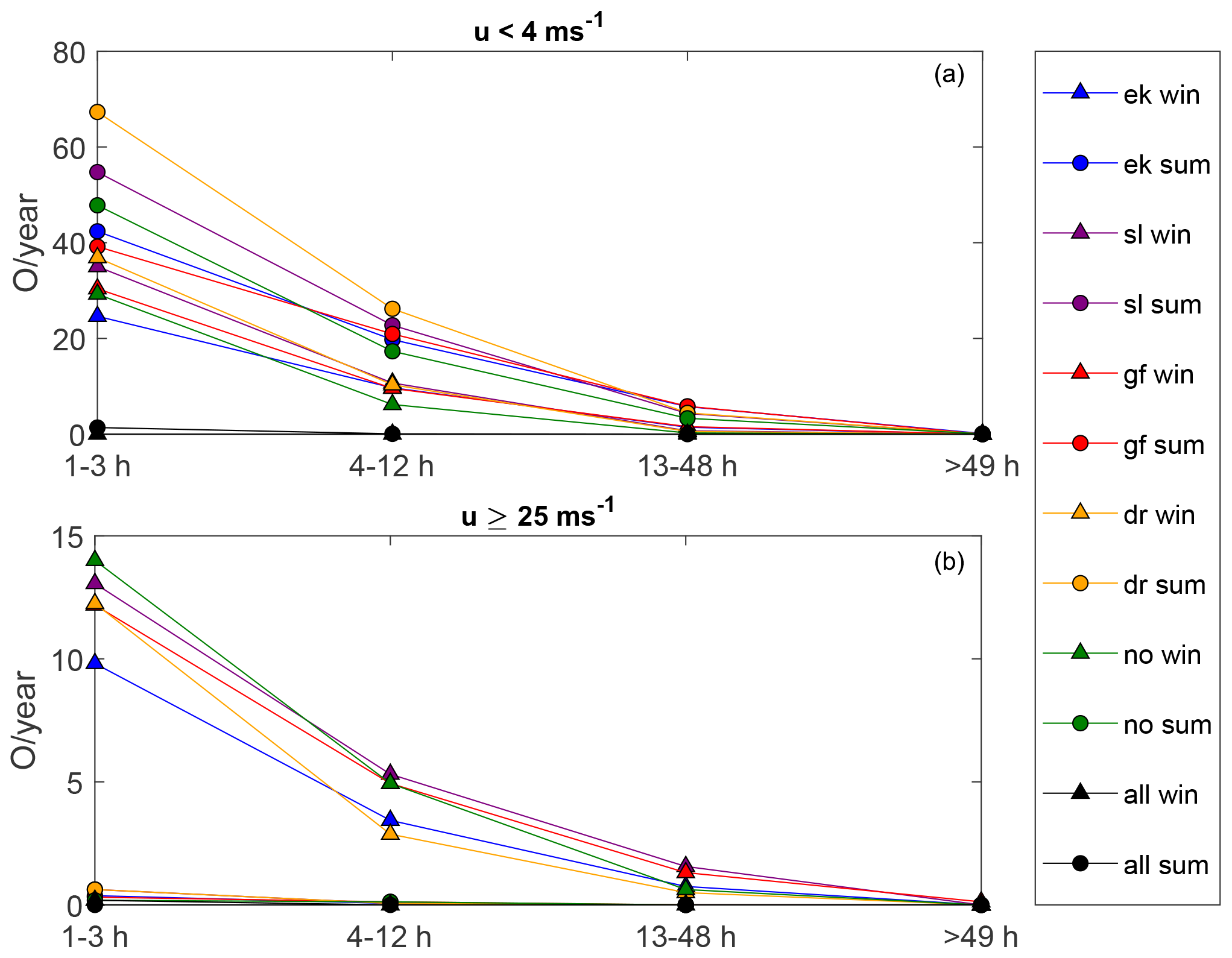
Figure 10Average number of yearly occurrences (O per year) of zero wind power production for different durations (1–3, 4–12, 13–48, and >49 h) both for u<4 m s−1 (a) and for u≤25 m s−1 (b). The occurrence of zero power is plotted for winter (triangles) and summer (circles), where the largest differences are seen.
The first thing to notice is that the occurrence of zero events decreases as the duration increases. In addition, the occurrence of zero events has almost ceased when all the sites are connected (black curve), and the reduction is most distinct for the shortest duration (1–3 h). More zero events are caused by too low wind (a total of 684.5 yearly zero events for all the sites) than too high wind (102.75). The occurrence of zero events caused by too high wind (too low wind) is highest during winter (summer). In addition, we see that the seasonal difference is largest for the zero events resulting from too high winds, where the occurrence during the winter is of a larger magnitude than during the summer.
To explain the seasonal differences in the occurrence of zero events, it is necessary to examine the main driving force of variability in the weather phenomena over the open ocean. Synoptic high- and low-pressure systems give rise to the changing weather at our specific sites and are the main contributor to weather variability over the open ocean. Winds strong enough to terminate power production (u≥25 m s−1) are often associated with the passage of intense low-pressure systems and their accompanying fronts. The occurrence of such strong wind events is more likely to take place during winter than during summer at the latitudes in question (Serreze et al., 1997; Trenberth et al., 1990). Throughout the year, differences in solar insolation give rise to an increased meridional temperature gradient during the northern hemispheric winter. These winter conditions result in a stronger background flow that favors low-pressure activity. On the other hand, the lack of these strong low-pressure systems during summer is probably the main reason why the occurrence of zero events caused by too low wind is highest during summer. In addition, the fact that blocking high-pressure events are more likely during spring also contributes to the seasonal difference in the too-low-wind events (Rex, 1950).

Figure 11Average (composite mean) large-scale situations (a, b) and the corresponding standard deviations (c, d) corresponding to for the site pair Ekofisk + Sleipner (ek + sl). The upper and lower rows correspond to caused by too low wind (u<4 m s−1) and too high wind (u≥25 m s−1), respectively.
4.6 Atmospheric conditions causing long-term power shutdown
The previous section demonstrated that the occurrence and duration of zero events are sensitive to the season and the atmospheric state. Klink (2007) has related long-lasting above- or below-average mean monthly values to variability in selected large-scale atmospheric circulation patterns. This section more closely examines surface pressure patterns associated with zero events lasting longer than 12 h using NORA10-reanalysis data (Reistad et al., 2011).
Surface pressure is a key quantity that contains considerable information about the atmospheric structure in the lower atmosphere. Figures 11 and 12 present the average surface pressure conditions (composite mean) and the corresponding standard deviation associated with zero events due to too low wind (u<4 m s−1) and too strong wind (u≥25 m s−1) for the two site combinations ek + sl and dr + no, respectively. The average atmospheric condition (comprised of 360 maps) resulting in too low wind speed for ek + sl is a high-pressure system extending from the North Sea and into the Norwegian Sea. This pattern is similar to the positive phase of the Scandinavia pattern (SCAND) (Barnston and Livezey, 1987). The variability given by the standard deviation (SD) is only a few hectopascals, indicating that the atmospheric patterns causing too-low-wind events are relatively similar to each other and that most of the variability lies in the patterns' extension towards the west. By contrast, the average atmospheric situation (comprised of 15 maps) due to too strong wind is an intense low-pressure system hitting the northwest coast of southern Norway, bringing tight isobars and strong winds over Sleipner (sl) and Ekofisk (ek). This situation is similar to the positive phase of the North Atlantic Oscillation (NAO). The SD is large in the center of the low-pressure system. The small spatial extension of the maximum standard deviation indicates uncertainty regarding the depth of the system. However, the SD is less over Ekofisk (ek) and Sleipner (sl), indicating that these sites seem to be located to the south of the extratropical cyclone where the strongest winds are often found.
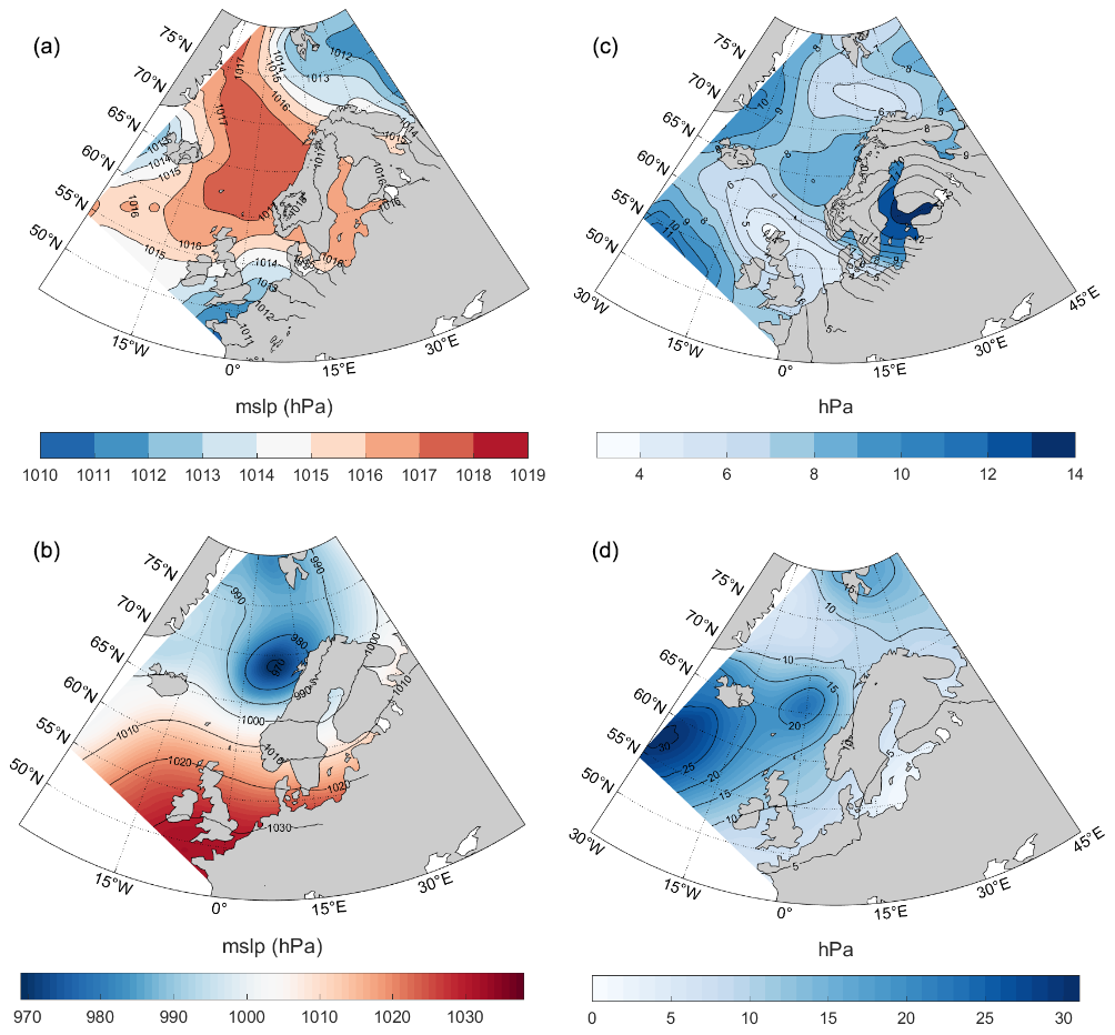
Figure 12Same as in Fig. 11, but for the site pair Draugen + Norne (dr + no).
Figure 12 contains the same information as in Fig. 11, but for the site combination Draugen + Norne (dr + no). The average atmospheric condition (comprised of 159 maps) caused by too low wind is different from that in Fig. 11a. The typical atmospheric condition here is a high-pressure system covering the entire Norwegian Sea and extending across Norway and into eastern Europe. The SD states that the eastern extension of the high-pressure system is unclear, giving rise to the large uncertainty east of Norway. Again, as in the case of too high wind for ek + sl, the site combination dr + no is located to the south of a strong low-pressure system (panel b). For dr + no, the mean system is now situated off the coast of northern Norway. The corresponding SD is large, indicating that several positions and strengths of the strong low-pressure system can cause situations with too high winds for dr + no.
Even though Kempton et al. (2010) investigated only four specific meteorological situations giving high and low collective wind power, our results are in line with theirs. As for the too-low-wind events in this study, the episodes of too low wind power in Kempton et al. (2010) were associated with a high-pressure system located in the vicinity of the wind power production sites. On the other hand, the episodes resulting in high collective wind power output in Kempton et al. (2010) were characterized by a low-pressure system located in the vicinity of the production sites. This is more or less in line with the results of this paper: our too-high-wind events are caused by intense low-pressure systems. Accordingly, a less intense low-pressure system will result in high-wind-power events.
In this study we quantified the effect of collective offshore wind power production using five sites on the Norwegian continental shelf, which constitutes a unique set of hourly wind speed data observed over a period of 16 years. The sites extend from Ekofisk in the south (56.5∘ N) to Sleipner, Gullfaks C, Draugen, and Norne in the north (66.0∘ N). See Fig. 1 and Table 1 for site details. We addressed the well-known intermittency problem of wind power by means of a hypothetical electricity cable connecting different configurations of the sites. The achieved smoothing effect was quantified by investigating the correlation between the sites as a function of the distance (km) and time lag (h) between the different pairs of site combinations. In addition, we studied the potential reduction of critical events (zero wind power-events) for different site combinations. Moreover, we investigated further details of zero events grouped into the two categories of too low and too high wind speed and the corresponding seasonal variations. Finally, the typical atmospheric patterns resulting in zero events caused by too low and too high wind speed for certain site combinations were studied. Our main findings are as follows.
-
In the case of all five sites, the wind climate was classified as superb (category 7), which corresponds to a potential of producing more than 400 W m−2 of wind energy (Zheng et al., 2016). The mean wind speeds at 100 m a.s.l. range from 9.97 to 11.25 m s−1 for Draugen and Norne, respectively.
-
Sleipner is the site that most frequently operates at rated power, 31 % of the time. This is due to the fact that Sleipner has an optimal combination of the scale and shape parameter, with the largest portion of the wind speed distribution falling between 13 and 25 m s−1.
-
The wind power variability, expressed as IQR and RCoV, ranges from IQR=0.89 to 0.95 for Norne–Ekofisk and Draugen and RCoV=0.90 to 1.00 for Draugen and Norne. Both IQR and RCoV decrease quickly with increasing array size of connected sites, indicating that wind power intermittency is reduced when sites are connected.
-
The pairwise correlation between sites drops off quickly as the distance between the sites increases. However, after ≈800 km the correlation is reduced to 0.1 and continues to decrease more slowly with increasing distance. Reaching this slowdown in the relation between correlation and separation distance after ≈800 km indicates that combining sites farther apart for further variability reduction has an almost negligible effect on the length scales possible to explore here.
-
The decorrelation length L shows that at a distance L≈400 km the correlation between site pairs has dropped to . This means that combining sites with at least a decorrelation length apart will substantially reduce wind power intermittency.
-
The decorrelation length L increases with variability timescale. Hence, if two of the offshore wind-power-producing sites were to balance each other at shorter timescales (<1 h), the separation distance would decrease (L<400 km).
-
To ensure a time lag of 10 h, from one site experiencing a certain wind event to the other connected site experiencing the same wind event, the separation distance needs to exceed ≈600 km.
-
Given a pairwise site connection, the separation distance exceeds ≈600 km to ensure a median wind power production of 25 % of installed capacity at one site when the production at the other site is zero.
-
The risk of having zero wind power for a given hour decreases from interval 8.0 %–11.2 % for the individual sites to less than 4 % when two sites are connected. Increasing the array size further reduces the risk, but the reduction is smaller.
-
The occurrence of zero events for a given site decreases as the duration increases. Thus, the shorter zero events (1–3 and 4–12 h) are more likely to occur than the zero events lasting longer (more than 13 h).
-
For a single site, the total yearly occurrence of zero events caused by too low wind (high wind) is 684.5 h (102.75 h). By comparison, when all the sites are connected, the total yearly occurrence of zero events is 1.5 and 0.2 h for too low and too high wind, respectively.
-
The occurrence of zero-power events caused by too high winds (too low winds) is highest during the winter months (summer months). This is due to the increased (decreased) occurrence of strong low-pressure systems at midlatitudes during the winter (summer).
-
The average atmospheric pattern resulting in too strong winds is a low-pressure system located to the north of the combined sites in question. This position of the system leaves the connected pair to the south of the core center where the strongest winds are usually found in an extratropical cyclone. By contrast, the atmospheric situation resulting in too low winds is a high-pressure system positioned over the connected sites, resulting in very calm wind conditions.
This research paper has first of all showed that by connecting wind power production sites the unwanted events like intermittency and zero events are reduced. The results obtained here are of great importance and lead us to some open questions:
-
Given that all locations in the North Sea and the Norwegian Sea could be used for wind power production, where are the best sites for interconnection in terms of (a) reducing intermittency and (b) maximizing power output?
-
Is the correlation between production sites largest in the east–west or the north–south direction?
-
Should the installed capacity at each production site be unequal in terms of (a) reducing intermittency and (b) maximizing power output?
The observational data for the sites used in this study can be retrieved at https://seklima.met.no/observations/ (last access: November 2020) (Norsk Klimaservicesenter, 2020) or at https://frost.met.no/index.html (last access: November 2020) (Meteorologisk Institutt, 2020).
IMS and NKG conceptualized the ideas, goals, and overarching research questions. IMS and AS carried out the data curation and formal analysis with the relevant statistics according to the corresponding methodology. NGK was responsible for the funding acquisition. IMS was responsible for the retrieval of the data and programming software, in addition to the validation and visualization of research results, with contributions from AS. IMS provided the original draft with the contribution from NGK, while all the authors contributed to the review and editing process. NGK and AS were responsible for the supervision.
The authors declare that they have no conflict of interest.
We thank the Meteorological Institute, and we in particular thank Magnar Reistad, Øyvind Breivik, Ole Johan Aarnes, and Hilde Haakenstad for providing all the data used in this study. We are grateful to David B. Stephenson for discussion of relevant statistics.
This work was funded through a PhD grant from Bergen Offshore Wind Center (BOW), University of Bergen.
This paper was edited by Joachim Peinke and reviewed by two anonymous referees.
Archer, C. L. and Jacobson, M. Z.: Supplying baseload power and reducing transmission requirements by interconnecting wind farms, J. Appl. Meteorol. Clim., 46, 1701–1717, https://doi.org/10.1175/2007JAMC1538.1, 2007. a, b
Barnston, A. G. and Livezey, R. E.: Classification, seasonality and persistence of low-frequency atmospheric circulation patterns, Mon. Weather Rev., 115, 1083–1126, https://doi.org/10.1175/1520-0493(1987)115<1083:CSAPOL>2.0.CO;2, 1987. a
Barstad, I., Sorteberg, A., and Mesquita, M. D. S.: Present and future offshore wind power potential in northern Europe based on downscaled global climate runs with adjusted SST and sea ice cover, Renew. Energ., 44, 398–405, https://doi.org/10.1016/j.renene.2012.02.008, 2012. a
Berge, E., Byrkjedal, Ø., Ydersbond, Y., and Kindler, D.: Modelling of offshore wind resources. Comparison of a meso-scale model and measurements from FINO 1 and North Sea oil rigs, in: European Wind Energy Conference and Exhibition EWEC, 16–19 March 2009, Marseille, France, 2009. a
Bosch, J., Staffell, I., and Hawkes, A. D.: Temporally explicit and spatially resolved global offshore wind energy potentials, Energy, 163, 766–781, https://doi.org/10.1016/j.energy.2018.08.153, 2018. a
Czisch, G. and Ernst, B.: High wind power penetration by the systematic use of smoothing effects within huge catchment areas shown in a European example, Windpower, 2001. a
Dvorak, M. J., Stoutenburg, E. D., Archer, C. L., Kempton, W., and Jacobson, M. Z.: Where is the ideal location for a US East Coast offshore grid?, Geophys. Res. Lett., 39, 1–6, https://doi.org/10.1029/2011GL050659, 2012. a, b, c, d
Emeis, S.: Wind Energy Meteorology, 2nd Edn., Springer, 2018. a
Grams, C. M., Beerli, R., Pfenninger, S., Staffell, I., and Wernli, H.: Balancing Europe's wind-power output through spatial deployment informed by weather regimes, Nat. Clim. Change, 7, 557–562, https://doi.org/10.1038/NCLIMATE3338, 2017. a, b
Jaffe, R. L. and Taylor, W.: The Physics of Energy, Cambridge University Press, Cambridge, https://doi.org/10.1017/9781139061292, 2019. a
Kahn, E.: The reliability of distributed wind generators, Elect. Power Syst. Res., 2, 1–14, https://doi.org/10.1016/0378-7796(79)90021-X, 1979. a, b
Katzenstein, W., Fertig, E., and Apt, J.: The variability of interconnected wind plants, Energy Policy, 38, 4400–4410, https://doi.org/10.1016/j.enpol.2010.03.069, 2010. a
Kempton, W., Pimenta, F. M., Veron, D. E., and Colle, B. A.: Electric power from offshore wind via synoptic-scale interconnection, P. Natl. Acad. Sci. USA, 107, 7240–7245, https://doi.org/10.1073/pnas.0909075107, 2010. a, b, c, d, e, f, g, h, i
Klink, K.: Atmospheric circulation effects on wind speed variability at turbine height, J. Appl. Meteorol. Clim., 46, 445–456, https://doi.org/10.1175/JAM2466.1, 2007. a
Lee, J. C. Y., Fields, M. J., and Lundquist, J. K.: Assessing variability of wind speed: comparison and validation of 27 methodologies, Wind Energ. Sci., 3, 845–868, https://doi.org/10.5194/wes-3-845-2018, 2018. a, b
Meteorologisk Institutt: What is Frost?, available at: https://frost.met.no/index.html, last access: November 2020. a
Norsk Klimaservicesenter: Seklima Observasjoner og værstatistikk, available at: https://seklima.met.no/observations/, last access: November 2020. a
Reichenberg, L., Johnsson, F., and Odenberger, M.: Dampening variations in wind power generation-The effect of optimizing geographic location of generating sites, Wind Energy, 17, 1631–1643, https://doi.org/10.1002/we.1657, 2014. a, b, c, d
Reichenberg, L., Wojciechowski, A., Hedenus, F., and Johnsson, F.: Geographic aggregation of wind power – an optimization methodologyfor avoiding low outputs, Wind Energy, 20, 19–32, https://doi.org/10.1002/we.1987, 2017. a, b, c, d, e, f
Reistad, M., Breivik, Ø., Haakenstad, H., Aarnes, O. J., Furevik, B. R., and Bidlot, J.-R.: A high-resolution hindcast of wind and waves for the North Sea, the Norwegian Sea, and the Barents Sea, J. Geophys. Res., 116, C05019, https://doi.org/10.1029/2010JC006402, 2011. a, b
Rex, D. F.: Blocking Action in the Middle Troposphere and its Effect upon Regional Climate, Tellus, 2, 275–301, https://doi.org/10.3402/tellusa.v2i4.8603, 1950. a
Serreze, M. C., Carse, F., Barry, R. G., and Rogers, J. C.: Icelandic low cyclone activity: Climatological features, linkages with the NAO, and relationships with recent changes in the Northern Hemisphere circulation, J. Climate, 10, 453–464, https://doi.org/10.1175/1520-0442(1997)010<0453:ILCACF>2.0.CO;2, 1997. a
Siemens AG: Siemens 6.0 MW Offshore Wind Turbine, Tech. rep., available at: https://www.qualenergia.it/sites/default/files/articolo-doc/6_MW_Brochure_Jan.2012_0.pdf (last access: November 2020), 2011. a
Sinden, G.: Characteristics of the UK wind resource: Long-term patterns and relationship to electricity demand, Energy Policy, 35, 112–127, https://doi.org/10.1016/j.enpol.2005.10.003, 2007. a, b
St. Martin, C. M., Lundquist, J. K., and Handschy, M. A.: Variability of interconnected wind plants: Correlation length and its dependence on variability time scale, Environ. Res. Lett., 10, 44004, https://doi.org/10.1088/1748-9326/10/4/044004, 2015. a, b, c, d, e, f
Trenberth, K. E., Large, W. G., and Olson, J. G.: The Mean Annual Cycle in Global Ocean Wind Stress, J. Phys. Oceanogr., 20, 1742–1760, https://doi.org/10.1175/1520-0485(1990)020<1742:tmacig>2.0.co;2, 1990. a
Vasilyev, L., Christakos, K., and Hannafious, B.: Treating wind measurements influenced by offshore structures with CFD methods, Energy Procedia, 80, 223–228, https://doi.org/10.1016/j.egypro.2015.11.425, 2015. a
Zheng, C. W., Li, C. Y., Pan, J., Liu, M. Y., and Xia, L. L.: An overview of global ocean wind energy resource evaluations, Renew. Sustain. Energ. Rev., 53, 1240–1251, https://doi.org/10.1016/j.rser.2015.09.063, 2016. a, b