the Creative Commons Attribution 4.0 License.
the Creative Commons Attribution 4.0 License.
 | 22 Dec 2020
Determination of the angle of attack on a research wind turbine rotor blade using surface pressure measurements
Rodrigo Soto-Valle
Sirko Bartholomay
Jörg Alber
Marinos Manolesos
Christian Navid Nayeri
Christian Oliver Paschereit
In this paper, a method to determine the angle of attack on a wind turbine rotor blade using a chordwise pressure distribution measurement was applied. The approach used a reduced number of pressure tap data located close to the blade leading edge. The results were compared with the measurements from three external probes mounted on the blade at different radial positions and with analytical calculations. Both experimental approaches used in this study are based on the 2-D flow assumption; the pressure tap method is an application of the thin airfoil theory, while the probe method applies geometrical and induction corrections to the measurement data.
The experiments were conducted in the wind tunnel at the Hermann Föttinger Institut of the Technische Universität Berlin. The research turbine is a three-bladed upwind horizontal axis wind turbine model with a rotor diameter of 3 m. The measurements were carried out at rated conditions with a tip speed ratio of 4.35, and different yaw and pitch angles were tested in order to compare the approaches over a wide range of conditions.
Results show that the pressure tap method is suitable and provides a similar angle of attack to the external probe measurements as well as the analytical calculations. This is a significant step for the experimental determination of the local angle of attack, as it eliminates the need for external probes, which affect the flow over the blade and require additional calibration.
- Article
(7701 KB) - Full-text XML
- BibTeX
- EndNote


The angle of attack (AoA) is, by definition, a 2-D concept. Nevertheless, on a wind turbine, the rotating system, i.e., a blade, is under 3-D effects such as tip and root vortices, yaw misalignment and velocity inductions, among others that render the precise determination of the AoA difficult (Shen et al., 2009). Additionally, the AoA is indirectly obtained through pressure or velocity fields; thus several uncertainties are added in its estimation. In this way, determining the local AoA on wind turbine blades remains one of the greatest aerodynamic challenges. At the same time, the determination of AoA is necessary in order to calculate lift and drag forces over the blade, develop accurate aeroelastic models, or establish a control tool.
The AoA can be calculated according to its geometrical definition using the velocity triangle defined by the wind velocity and the rotational speed. Unfortunately, this estimation relies on well-known free-stream conditions and does not take into account induction effects. Therefore, if a more reliable estimation is required, it is necessary to use on-blade measurement tools.
Most of the on-blade measurements use external probes to measure the local pressure. Various methods have been used, while they follow the same principle: apply a correction due to the upwash induced by the presence of the blade itself. Including a stagnation pressure hole leaves the three-hole probe as required minimum. Additional holes (five, six, seven) allow the cross flow derivation and provide better accuracy. However, the number of calibration curves increases; thus the determination of the inflow becomes more difficult (Schepers and Van Rooij, 2005).
Several field measurements have been conducted using probes as one of the estimation methods for the AoA. Brand et al. (1997), Simms et al. (1999), Madsen et al. (1998), Maeda et al. (2005) and Bak et al. (2011) showed measurement results employing five-hole probes from the Energy research Centre of Netherlands (ECN), the National Renewable Energy Laboratory (NREL), Technical University of Denmark (DTU), Mie University (Mie) and DanAero projects, respectively (see Table 1). Bruining and van Rooij (1997) used three-hole probes in the Delft University of Technology (DUT) project. The upwash correction was made based on wind tunnel measurement of static blade or airfoils representative of the studied blade section. It is remarkable that the case of the ECN exhibited better results without the upwash correction. This is assumed to be the compensation effect of the downwash from the shed vorticity due to the variation in the bound circulation along the blade span (Schepers et al., 2002).
Brand et al. (1997)Bruining and van Rooij (1997)Simms et al. (1999)Madsen et al. (1998)Maeda et al. (2005)(Bak et al., 2011)Schepers et al. (2012)Sicot et al. (2008)Klein et al. (2018)Moscardi and Johnson (2016)Table 1Angle-of-attack estimation methods on wind turbine rotor blades.

a Rec: Reynolds number based on chord length at 70%R and relative inflow velocity. b Additional information can be found on the International Energy Agency (IEA) Annexes reported by Schepers et al. (1997) and Schepers et al. (2002). c Summarized in the IEA Annexes reported by Schepers et al. (2002). d Reported by Schepers and Schreck (2019).
These methodologies have been applied over wind turbine models on tunnel experiments. Gallant and Johnson (2016) presented the determination of the AoA using a five-hole probe on a three-bladed turbine model at the University of Waterloo (UW) wind tunnel facilities. A combination of geometrical and induction corrections, based on the work of Hand et al. (2001), was applied to obtain the AoA for different yaw offsets and tip speed ratios. The results show a good trend agreement between the probe measurements and the model proposed by Morote (2016). The operation range of the five-hole probe was studied by Moscardi and Johnson (2016) for a large range of pitch and yaw angles (±50∘), using the test rig with only one blade.
Bartholomay et al. (2018) showed AoA estimation through three-hole probes, from the Berlin Research Turbine (BeRT). The three-hole-probe calibration was made under axial inflow and performed on-blade operation for axial and yawed inflows up to 30∘. The results showed a good agreement with computational fluid dynamics (CFD) computations (Klein et al., 2018) under the same operation points.
In general, according to the published literature, external probes can be used to determine the AoA. However, in the case of wind turbine models, such probes are intrusive and significantly disturb the flow over the blade section where they are mounted.
Other complementary tools used on research turbines are surface pressure sensors, located along the blade chord. These sensors are used to record the pressure distribution along the blade chord at a desired radial position and to calculate the aerodynamic loads. Different computational methods use this information as a source to estimate the AoA.
The inverse blade element momentum (BEM) method is probably the most common. From the surface pressure sensors, the normal and tangential forces are calculated, assuming that they are uniform over an annulus containing the blade section. The wake-induced velocities are calculated according to momentum theory, yielding the effective velocity vector and subsequently the AoA (Whale et al., 1999). This method was implemented by ECN, NREL and DTU projects, obtaining similar results with their respective estimations based on probes.
The NREL suggested an algorithm to estimate the AoA from pressure distribution values under axial (Sant et al., 2006a), unsteady (Sant et al., 2006b) and yawed conditions (Sant et al., 2009). The method assumes an initial AoA distribution. The lift is then calculated for each azimuth and radial position based on the pressure surface data and the AoA. Afterwards, the bound circulations were determined by means of the Kutta–Joukowski theorem for a lifting line. The resulting values were prescribed in a free-wake vortex model to obtain a new AoA based on the induced velocities to finally iterate until the AoA converged.
Schepers et al. (2012) presented the inverse free-wake method applied to the MEXICO rotor, which follows the same BEM principle but using the normal and tangential forces into a free-wake model. Several computational methods can be found in the latest phase of the project, summarized by Schepers et al. (2018), such as azimuth average, three-point and lifting line average methods among others.
The surface pressure measurements also allow experimental estimations. Shipley et al. (1995) showed the stagnation point normalization method described as follows: the local dynamic pressure is estimated as the maximum value of the pressure side in each pressure distribution station. This value is used to estimated the free-stream velocity and then the AoA based on the geometrical velocities defined by pitch, yaw and azimuth angles.
Moreover, Brand (1994) presented the stagnation point method. The AoA is estimated as follows: the stagnation point is located as the previous method. Afterwards, the intersection of the chord line and a line normal to the surface at the stagnation point is used to estimate AoA. The position of the point of intersection can be determined using 2-D approaches, either codes or wind tunnel measurement (Whale et al., 1999). The drawback of this method is that it relies only on the geometry of the blade section, assuming AoA and Reynolds number have no influence.
Furthermore, Bruining and van Rooij (1997) exposed an additional method that uses two frontal pressure taps, one on the pressure side and one on the suction side, working as a built-in probe in the blade. The drawback of this is that it requires calibration of the blade station where the taps are located.
Schepers et al. (2002) reported the comparison between experimental probes, pressure taps and inverse BEM methods regarding the field measurement from ECN, NREL, DUT, DTU and Mie. The main conclusions found were (1) the ambiguity of the 3-D AoA definition implies that any check on accuracy can only be carried out with an arbitrary reference; (2) before stall, the estimations of the AoA remain with differences below 1∘; and (3) above stall conditions, the differences between methods can go up to 4∘. Table 1 shows field and wind tunnel experiments with the most common estimation methods mentioned above.
Therefore, the pressure distribution over a rotating section can be used to relate the AoA, if it is comparable with nonrotating conditions, where the AoA is known. Several investigations showed a relation between 2-D and 3-D pressure distribution. Ronsten (1992) showed a good agreement between the pressure distribution over nonrotating and rotating blades along span positions of and at tip speed ratios of 4.32 and 7.37, respectively.
Guntur and Sørensen (2012) presented different methods to determine the AoA for the MEXICO rotor (Bechmann et al., 2011) based on CFD data. One of the approaches is based on matching up CP distributions from 2-D and 3-D data, where the AoA was known in the former case. This method has a good agreement for small angles of attack (<10∘) and in the middle blade region (). The latter points out an alternative method to estimate the AoA where the 2-D and 3-D pressure distribution are comparable.
Maeda et al. (2005) showed surface pressure comparison between field measurements and wind tunnel experiments. The latter was carried out using the same blade in stationary conditions. A good agreement was shown, regarding the surface pressure distribution under prestall (AoA=10∘) and stall (AoA=16∘) conditions. In the case of a poststall (AoA=20∘) condition, the results of the wind tunnel present a reduced pressure magnitude on the suction side, in contrast with the field case.
Bak et al. (2011) studied the pressure distribution on a wind turbine in atmospheric conditions and in a wind tunnel. The wind tunnel experiments were carried out with 2-D wing, taking the characteristics of four specific sections from the turbine. The agreement remains valid for small angles of attack (<12∘) and for the outer region of the blade ().
Overall, it is generally agreed that static 2-D wings and rotating blades have a good agreement in surface pressure measurements, at least for attached flow conditions. This opens up the possibility of using methods based on the blade chord pressure distribution to estimate the AoA, in the range of agreement.
Gaunaa (2006) developed an analytical solution for the unsteady 2-D pressure distribution on a variable geometry airfoil undergoing arbitrary motion, based on thin airfoil theory. Further investigations made by Gaunaa and Andersen (2009), using this method, related the pressure over the airfoil with the effective AoA. The added benefit of the specific method is its simplicity, as it only requires the pressure difference between the airfoil pressure and suction side at one or two chordwise positions and at the same time can be performed while operating in unsteady conditions.
To the authors' knowledge, this method has not been applied on a rotating blade yet. Given the good agreement between 2-D and 3-D pressure distributions away from the root region, this paper presents an alternative method of determining the AoA by means of pressure tap measurements. The present investigation aims at providing experimental verification for one such surface pressure method (Gaunaa and Andersen, 2009) on the rotating blade.
Today, new technologies such as passive fiber optic pressure sensors presented by Schmid (2017) are able to perform quasistatic and unsteady measurements of rotor blades in operation that can withstand harsh conditions. Therefore, the development of new methods to determine the AoA based on pressure distribution data would provide valuable information without the necessity of invasive tools.
The Technical University of Berlin has developed a scaled wind turbine model, BeRT, equipped with three-hole probes and pressure taps on one of its blades (Vey et al., 2015). The results presented here are the first on-blade pressure measurements from the BeRT blade and can be used to validate numerical solvers and to develop future control strategies.
In the remainder of the paper, the facilities and the research turbine model are described, followed by the methodology to determine the AoA and to assess the validity of the Gaunaa method on the rotating plane. The results are presented in Sect. 4 and the paper closes with concluding remarks in Sect. 5.
2.1 Wind tunnel
The tests were conducted at the Hermann Föttinger Institut of the Technische Universität Berlin in the GroWiKa (large wind tunnel), a closed-loop wind tunnel driven by a 450 kW fan and a cross-sectional area m2 presented in Fig. 1 (left). The turbine model was placed at the large test section, where the maximum velocity is 10 m s−1. The setup was reproduced from the work of Bartholomay et al. (2017), in which the flow quality was measured and the reproducibility of the flow was evaluated. In order to keep the turbulence intensity on a comparable level, one homogeneous filter mat and three screens were positioned in the cross sections upstream of the turbine as can be seen in Fig. 1 (left). The turbulence intensity achieved with this setup is less than 1.5 %. With this level of turbulence, small variations between rotations of the turbine can be expected, which suggests using multiple rotations to achieve a significant statistical average in the data.
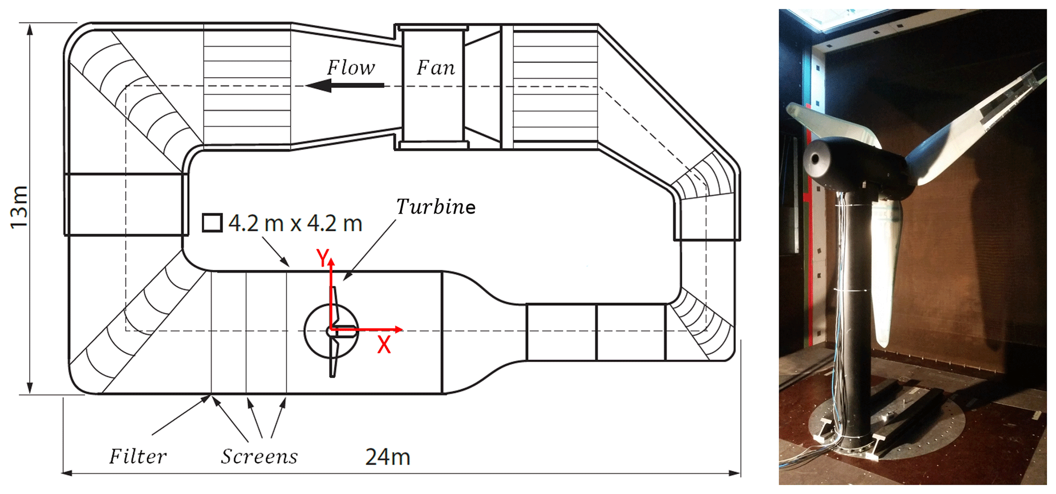
Figure 1Outline of GroWiKa, modified from Klein et al. (2018) (left). Berlin Research Turbine – BeRT in the wind box (right).
At the same time, the inflow showed some heterogeneity, i.e., was not fully uniform as is depicted in Fig. 2 (left). Figure 2 (right) shows four axial velocity distributions at the radial positions 45 %R, 65 %R, 75 %R and 85 %R. Therefore, due to these characteristics it was decided to analyze the measurement data over small azimuth angle stations.
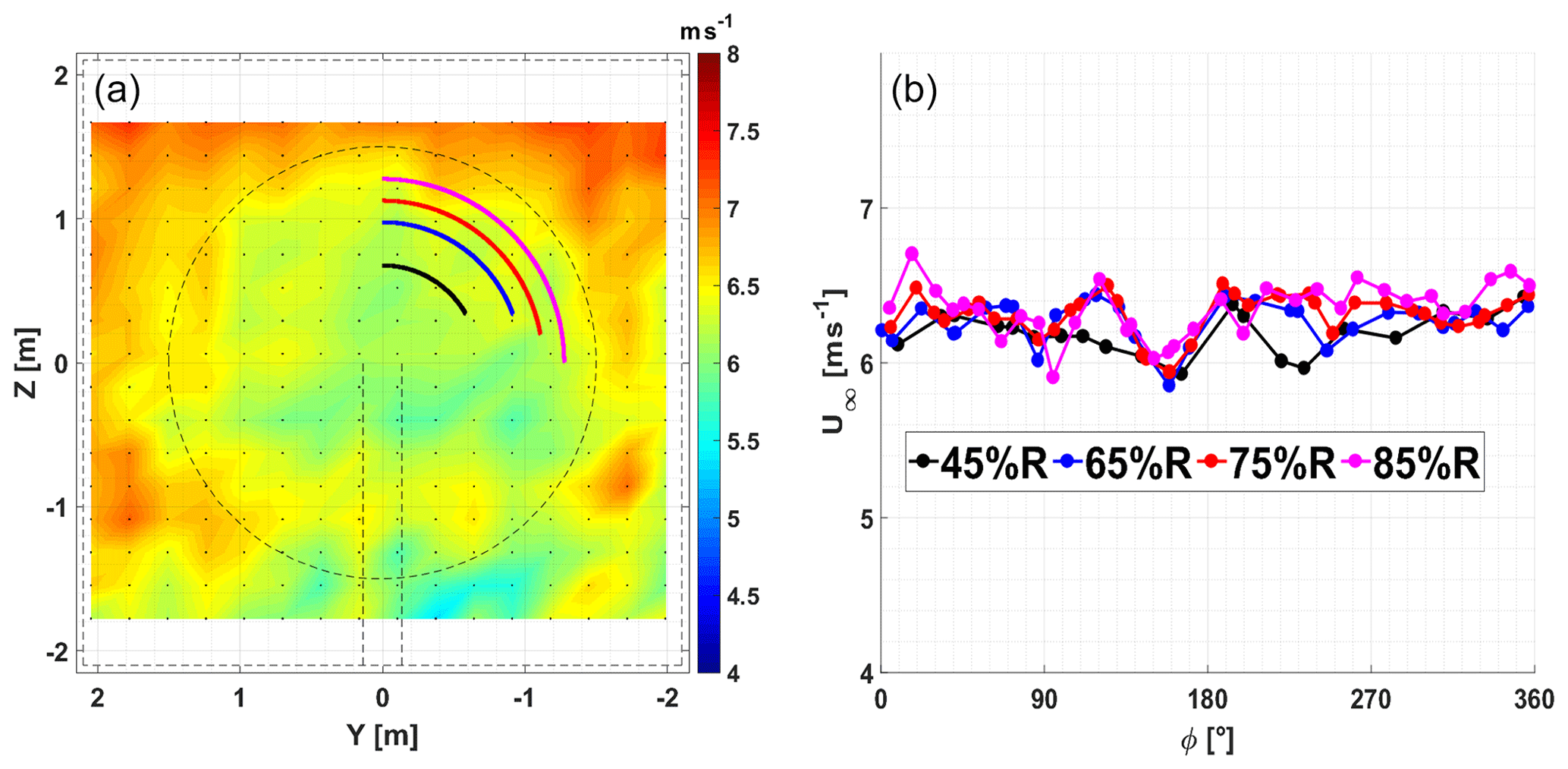
Figure 2Axial inflow. Dashed lines: tip and tower positions. Colored lines: radial positions at 45 %R, 65 %R, 75 %R and 85 %R following the blade rotation (a). Velocity distributions over radial positions at 45 %R, 65 %R, 75 %R and 85 %R (b).
Additionally, the dynamic pressure is monitored by two Prandtl tubes located at the walls at 0.43R upstream the turbine at 2.7 m height. Based on the Prandtl tubes, all test cases were conducted with a free-stream velocity of U∞≈6.5 m s−1.
2.2 Wind turbine model
BeRT, Fig. 1 (right), is a three-bladed upwind horizontal wind turbine with a rotor radius of R=1.5 m. The turbine yaw angle and the blade pitch angle were fixed during the measurements. Figure 3 (left) shows a reference sketch for the azimuth (ϕ) and yaw (ψ) angles.
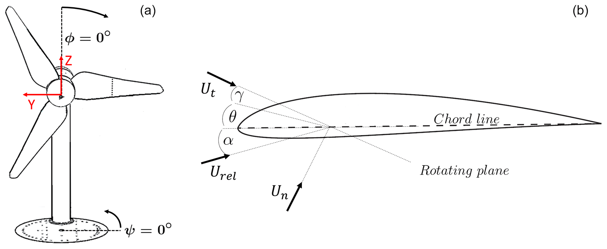
Figure 3Angle definition. Azimuth, ϕ, and yaw, ψ (a). Angle of attack, α; pitch, θ; and twist, γ. Ut, Un and Urel are the tangential, normal and relative velocities, respectively (b).
A slightly modified Clark Y airfoil profile is used along the entire blade span and there is no cylindrical root section. The airfoil modification was necessary in order to account for a realistic trailing edge thickness with respect to manufacturing requirements. Aerodynamically, the design intended to avoid stall while continuing to offer optimal performance and the maximum internal space to include instrumentation (Pechlivanoglou et al., 2015).
In this way, the specific airfoil profile was chosen as it performs well at low Reynolds numbers (Re), i.e., at the conditions relevant to BeRT (Re range of 1.7-3.0×10⁵ along the span). The blade twist was selected so that the local AoA stays constant over the span at rated conditions. Figure 3 (right) illustrates the definition of the main angles and velocities over a blade section, and Fig. 4 (left) shows the twist and chord distributions.
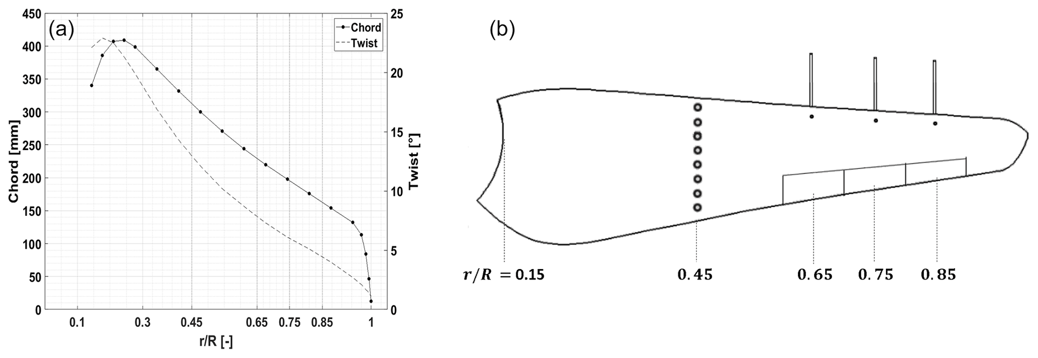
Figure 4Twist and chord distribution along span (a). The rotor blade with three-hole probes and pressure taps over span position (b).
The turbine rotor area (ABeRT) produces a considerable blockage ratio in the wind tunnel, . The blockage effect was analyzed in terms of the equivalent free-stream velocity (U′) which produces the same torque. Glauert (1926) showed that for a propeller the ratio between the wind tunnel velocity (U∞) and its corresponding equivalent free-stream velocity is a function of the blockage ratio and the thrust coefficient (CT), Eq. (1). Using the BeRT rotor characteristics reported by Marten et al. (2019), a thrust coefficient of CT=0.77 (expected at rated condition) was considered. Subsequently, applying Eq. (1), implemented on wind turbines, results in the velocity ratio of .
It is noted that this correction has also been applied successfully in wind tunnel experiments with an even higher blockage ratio (45 %; Refan and Hangan, 2012).
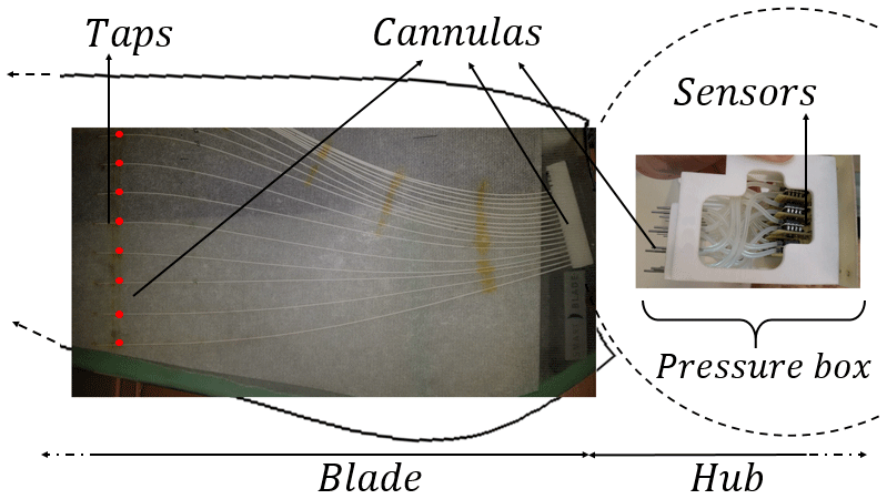
One blade was equipped with pressure taps and three three-hole probes at different radial positions, as shown in Fig. 4 (right). Due to manufacturing reasons (internal structure, hole spacing), the pressure taps could only be located at a single spanwise location, which was at 45 % of the blade span. Each pressure tap was connected through silicone tubes inside the blade to a pressure box located in the hub which contains all sensors. The average length for the tubes between tap and sensor was 650 mm which included an arrangement between cannulas and tubes as shown in Fig. 5.
The three-hole probes were located at 65%R, 75%R and 85%R and mounted on the pressure side (see Fig. 6, left). The three-hole probes consist of one straight tube in the middle, accompanied by two outer tubes with a 45∘ nozzle (see Fig. 6, right). Each outer tube was connected to a differential pressure sensor through a silicone tube, using the middle one as a reference. The sensors were installed at the spanwise position of each probe, reducing the tube length to less than 100 mm.

Figure 6Three-hole probes mounted in the equipped blade (a). Calibration of a three-hole probe and tip details (b). It is noted that although the flaps appear deflected in the photo, they were always in the neutral position for the experiments of this campaign.
All pressure transducers were installed in such a way that their membranes were parallel to the plane of rotation to minimize the centrifugal effect on them. More information about the sensors can be found in previous work by Vey et al. (2015), while the calibration and data acquisition procedure is detailed in the Sect. 3.1.
The blade was also provided with three trailing edge flaps with 10%R span length and 30%c chord length and located consecutively from 60 % to 90 % along the span. Each three-hole probe was aimed to give feedback information to choose flap movements. However, The flaps were fixed without any deflection for all test cases presented in this study. The turbulence transition was not fixed over the blades, in contrast to the previous work of Klein et al. (2018).
Rotating (NI cRIO-9068) and nonrotating (NI cDAQ-9188) measurement systems were synchronized and located in the hub and the external control cabinet, respectively. The measurement data were recorded using NI 9220 modules with an acquisition frequency of 10 kHz.
The pressure data from the blade were recorded through the rotating system, while the free-stream dynamic pressure was recorded through the nonrotating system. The blade position was recorded through a Hall effect sensor located in the nacelle. Each measurement was recorded and phase averaged until 100 rotations were completed, with an azimuth step of Δϕ=1∘.
In this section, the methodology of this research is described. The main idea is to compare the results obtained by the method proposed by Gaunaa and Andersen (2009) when it is applied to the pressure tap data against the AoA from the three-hole-probe measurements and analytical calculations.
According to the BeRT design specification, the combination of chord and twist distribution achieves an optimal shape (Pechlivanoglou et al., 2015) which provides a constant AoA over most of the blade span (Bartholomay et al., 2017), so the AoA at the radial position of the pressure taps and the three-hole probes should be the same under aligned flow conditions.
The calibration of the sensors, the applied corrections and the description of the methods used to determine the AoA follow, while the test cases and their uncertainty are summarized at the end of this section.
3.1 Calibration
Differential pressure sensors were used for both experimental methods, the pressure taps (HCL0025E) and the three-hole probes (HCL0075E). During the calibration of the sensors, the turbine was in a static position and a constant pressure was provided to achieve 11 calibration pressure points using the external calibrator, Halstrup KAL 84. All calibrations were linear and the fitting curves showed a coefficient of determination value of R2≥0.999.
The three-hole probes were calibrated in a small wind tunnel. The calibration range was from −30 to 30∘ with steps of 0.5∘. The calibration was carried out between the normalized pressure and the swept angles following the standard procedure described by Dudzinski and Krause (1969). Subsequently, the calibration was repeated for inflow velocities from 16 to 22 m s−1 with steps of ΔU=2 m s−1. The velocity range was selected so that it covers the relative velocity perceived by the blade in the range , i.e., the location of the three-hole probes. The AoA fit remains linear within −10 to 10∘, getting a nonlinear fit for larger angles.
3.2 Pressure correction
The pressure sensors measure the differential pressure (Psi). The three-hole probes use the inner tube as a reference, while the pressure taps use the static pressure in the test section.
The structural design of BeRT results in eigenfrequencies of the blades of fblade≥13.5 Hz and the tower of ftower≥18 Hz. For this reason, the data were low-pass-filtered using a Butterworth filter with a cutoff frequency of 12 Hz to reduce the noise and structural vibrations. Figure 7 shows the raw signal spectra over one three-hole-probe pressure sensor at 75%R and the pressure tap at x=2%c. It can be seen that the main variations are influenced by the rotational frequency of 3 Hz and its harmonics.
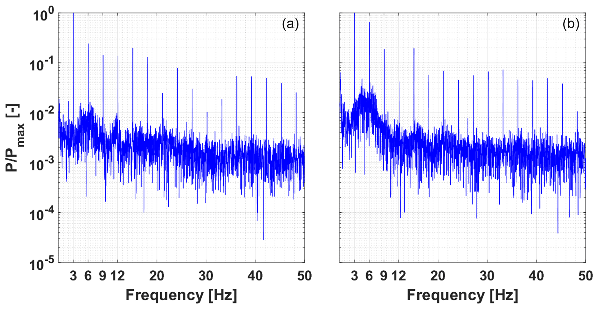
Figure 7Frequency spectrum of one pressure sensor of the three-hole probe at 75%R (a). Frequency spectrum of the pressure tap at x=2%c (b). Both cases are for a pitch angle of θ=0∘ and yaw angle of 0∘.
The dynamic response of the taps–tubes system was evaluated theoretically following the model proposed by Bergh and Tijdeman (1965). Figure 8 (left) shows a scheme of the model used to apply the analysis, based on the tube arrangement depicted in Fig. 5, while Fig. 8 (right) shows the theoretical response of the system, based on Bergh and Tijdeman (1965). In order to minimize the attenuation and phase lag of the signal, an additional low-pass filter was applied, with a cutoff frequency of 6 Hz. This was considered adequate as it shows the amplitude amplification and phase lag are less than 1 % and 10∘, respectively.
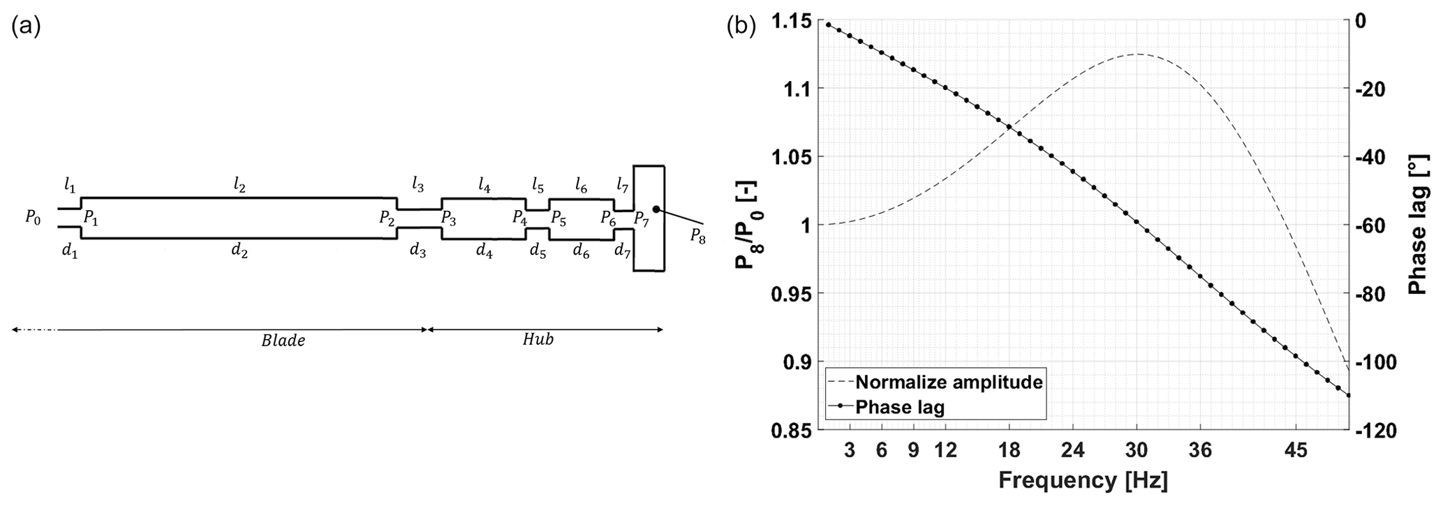
Figure 8Scheme of the model to apply Bergh and Tijdeman (1965) dynamic response analysis. P, l and d are the pressure, length and diameter of each section (a). Theoretical dynamic response of the amplitude and phase lag (b).
In the case of the pressure taps, the centrifugal effect was quantified and corrected, Eq. (2), based on Hand et al. (2001), where ri is the radial position of the pressure tap i and Ω is the turbine angular velocity, 2πf.
The hydrostatic correction has less impact since all the sensors are located in the hub and was consequently neglected.
3.3 Methods to determine the angle of attack
3.3.1 Three-hole probes
The method to determine the AoA from the three-hole probes was based on previous work with the same setup. It is outlined here for completeness, while further details can be found in Bartholomay et al. (2017). Figure 9 shows the reference system for an arbitrary blade section, with a three-hole probe installed.
The AoA relative to the probe, αprobe, was identified from the three-hole-probe calibration, through their normalized pressure, Eq. (3), where P1 and P2 are the outer tubes, P0 the reference tube and the average between the outer tubes.
However, as shown in Fig. 9, a geometrical rotation between the probe and the section coordinates was necessary to evaluate the AoA in the respective blade section, αprobe, section. The latter angle differs from α, which is the effective AoA of the blade section, because the blade itself induces a velocity on its surroundings. To correct this, XFOIL (Drela and Youngren, 2001) calculations were used to estimate the velocity at the probe location, under the assumption of 2-D flow. Afterwards, a fit function was found between the effective AoA, α, and αprobe, section. Equation (4) shows an approximation of the downwash correction (Klein et al., 2018).
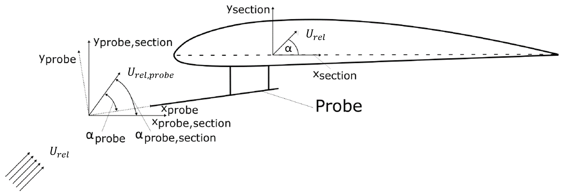
Figure 9Schematic of the reference system for a probe, modified from Klein et al. (2018).
As the turbine was set under yaw misalignments, it is important to verify the effectiveness of the 2-D probe. The range of the AoA, in the probe stations, is . Therefore, adding the corresponding twist angle, the range of the AoA relative to the probes is . Moreover, the probes are aligned with the chord; thus the yaw angle relative to the probe is the same .
Zilliac (1993) and Moscardi and Johnson (2016) determined the mono-zone as (αprobe, ψprobe). This zone represents where the calibration parameters of the probes remain invariant, i.e., CP, probe. These studies used probes with seven and five holes, respectively. As a three-hole-probe sweeps the same angle of these calibrations, its mono-zone should be the same.
Moreover, Bruining and van Rooij (1997) employed three-hole probes on field measurements with good agreement of the AoA, compared to inverse BEM and stagnation point methods. In addition, Klein et al. (2018) showed similar results from experimental and CFD simulations where the wind tunnel structure was considered. Therefore, based on these arguments, it was assumed that the three-hole probes are able to estimate the AoA in the yaw misalignments here studied.
3.3.2 Pressure taps
The determination of the AoA from the pressure distribution on the blade section was based on the unsteady model developed by Gaunaa (2006). The main assumptions for this methodology rely on the thin airfoil theory and low Mach number. This allows modeling of the airfoil as its camber line together with the assumptions of inviscid, incompressible and irrotational flow.
Aiming at simpler solutions to estimate airfoil loads that can be applied to active load control, and based on the considerations mentioned above, Gaunaa (2006) formulated an analytical expression for the forces over an arbitrary airfoil shape. This expression relates the pressure difference between the lower and upper sides, over the camber line, with the velocity potential field, aerodynamic forces and pitching moment. Gaunaa and Andersen (2009) summarized this formulation in Eq. (5) as the normalized pressure and its contributions, where ΔP(x) is the pressure difference between the lower and upper sides at a specific chordwise position and q=0.5ρU2 is the dynamic pressure.
It is important to note that this summary neglects the chord streamwise degree of freedom, i.e., .
On the right side of Eq. (5), gc(x) corresponds to the influence of the circulatory forces. This contribution is modulated by αc, eff, the effective AoA that takes into account the time lag effects caused by the vorticity shed into the wake, for simplicity, now considered α.
The remaining contributions in Eq. (5) depend on the instantaneous motion of the airfoil, known as added mass terms. The second and third terms, gcamb and , correspond to the added mass due to the basic camber line and pitching, respectively.
The formulation allows the calculation of the effect of a flap on the airfoil, with β being the flap angle. This contribution in the model is considered with the added mass term gβ. Since there is no flap at the 45 % span position, the flap deflection angle is set to β=0∘ and therefore gβ is eliminated.
The term gL contains the nonlinear contributions. Gaunaa and Andersen (2009) claim that the addition of the geometrical nonlinearities does not change the conclusions from linear estimation for most of the chord, except for a zone very close to the leading edge. Based on this consideration, the term gL is neglected.
Gaunaa and Andersen (2009) and Velte et al. (2012) suggested a control variable based only on two pressure taps. To achieve this, the contribution of the pitching-added mass term, was neglected by choosing a specific chord position where its value is zero.
Equation (6) shows the reduced relation between pressure distribution and AoA, where and . An extended review of the two-dimensional theory and the mathematical derivation of this method and applications can be found in Gaunaa (2002, 2006).
Several studies conducted by Gaunaa (2002), Gaunaa and Andersen (2009), and Velte et al. (2012) investigated the same theory on wing experiments and computational models, with a Risø-B1-18 and NACA64418. Thus, it is assumed that the linearity, applied to the remaining terms, is a good approximation for a Clark Y airfoil shape, which is thinner (11.8 %) than the other airfoils where the method was successfully applied.
In order to obtain the constants k1 and k2 from Eq. (6), XFOIL calculations were computed. The AoA was swept from −3 to 10∘. The Reynolds number () and free transition method () influence were studied with no significant changes. Subsequently, a linear curve fit was made between normalized pressure (ΔCP(0.125)) and the AoA swept. The fit values are k1=0.23 and k2=0.43, with a coefficient of determination of R2≥0.999.
Finally the AoA was calculated using Eq. (6), where .
Figure 10 shows a good agreement between the pressure distribution from the rotating blade and the computational tool in the estimated angle. The difference between both curves is ΔCP≤0.05 until x=30%c, except the peak at the suction side, . Afterwards, ΔCP varies between 0.05–0.10. This agrees with the fact that rotation does not have a great impact over the pressure distribution in the attached flow operation points (Ronsten, 1992; Corten, 2001).

Figure 10XFOIL (α=7.6∘) and measured pressure distribution of the current setup at a yaw angle of ψ=0∘, pitch angle of θ=0∘ and azimuth angle of ϕ=0∘.
Since there are no pressure taps in the exact 12.5%c position, a linear interpolation was made, between [10–15]%c for the suction side and [10–30]%c for the pressure side.
The relative dynamic pressure, , was considered equal to the maximum value in pressure side distribution, i.e., at the stagnation point (Shipley et al., 1995), for each azimuth station. This was required for the yaw misalignment cases, where the dynamic pressure is variable with azimuth position.
3.3.3 Analytic estimation
The introduction of a yaw misalignment produces an expected change in the AoA distribution along the blade span due to the crossflow, i.e., depends on the azimuth angle variations. Therefore, a geometrical approach was used to compare the experimental methods under these operational points, as pressure tap and three-hole-probe locations differ in radial position.
The normal velocity contribution is a function of the yaw angle, Eq. (7). Conversely, the tangential velocity contribution depends on the rotational speed, yaw and azimuth angle, Eq. (8), due to the crossflow presented (see Fig. 3). Using these geometrical velocity contributions and the axial, a, and tangential, a′, factors simulated with the BEM-module QBlade (Marten et al., 2015), an analytical AoA was estimated as is shown in Eq. (9).
The blockage effect must be considered. Consequently, the inflow velocity (U∞) for these calculations was replaced by the equivalent free-stream velocity. Thus, applying Eq. (1) results in the equivalent free-stream velocity of m s−1.
Equation (9) can be used to estimate the AoA in the aligned case, which is independent of the azimuth angle, as the yaw angle is zero. Therefore, the AoAs have small variations, regarding the induction factors. Thus, the AoA in the location of the pressure taps and three-hole probes takes the value of , when the pitch angle is set at θ=0∘.
3.4 Test cases and measurement uncertainty
Several operational conditions were analyzed, three yaw angles ψ=0, −15 and −30∘, and for each yaw angle, the pitch angle was swept from −2 to 6∘ in steps of Δθ=2∘. For all cases, the tip speed ratio was fixed λ=4.35.
The measurement uncertainty, for all quantities, was taken into account in order to quantify the error magnitude over the results. Both AoA estimation approaches have the same iteration in the error propagation, based on the following steps:
- 1.
nominal error of each sensor;
- 2.
the standard deviation of the averaged measurements, which was calculated with the same azimuth step as the phase average;
- 3.
conversion to AoA and thus the error propagation after applying Eqs. (3) and (6) for the three-hole probes and pressure taps, respectively.
Table 2 shows the overall uncertainty for all the quantities. Point 3 depends highly on the values of the measured pressure. For this reason, Table 2 shows the minimum and maximum values. An example of the uncertainty over the azimuth angle of each tool can be seen in Appendix D1.
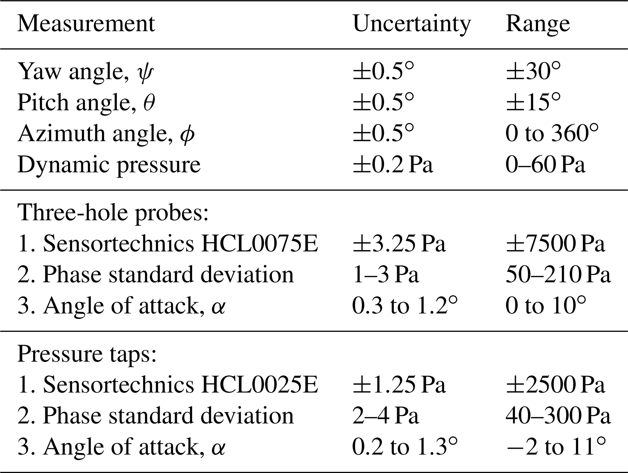
During the measurement campaign, while the changes on the pitch or yaw angle were made between test cases, the tunnel was left open to allow for fresh air to enter the tunnel circuit. As a result, the temperature and relative humidity were kept within 18±1.5 ∘C and 40±5 %, respectively. According to Tsilingiris (2008), these values represent small changes in the physical properties; thus, a density correction was neglected.
The results are presented in this section, starting from the pressure distributions and the relative dynamic pressure along the chord at the span position of r=45%R, followed by the comparison between the described methods to determine the AoA. Finally, an additional comparison is presented with the variations in the pitch angle.
4.1 Pressure distribution
The AoA estimation based on the surface pressure measurements depends on the relative dynamic pressure (qrel) and the pressure difference (ΔP(12.5%c)); see Eq. (6). It is hence important to examine their variation with azimuth position before proceeding to the AoA estimation. Figure 11 shows the variation in both variables normalized by the free-stream dynamic pressure Pa.
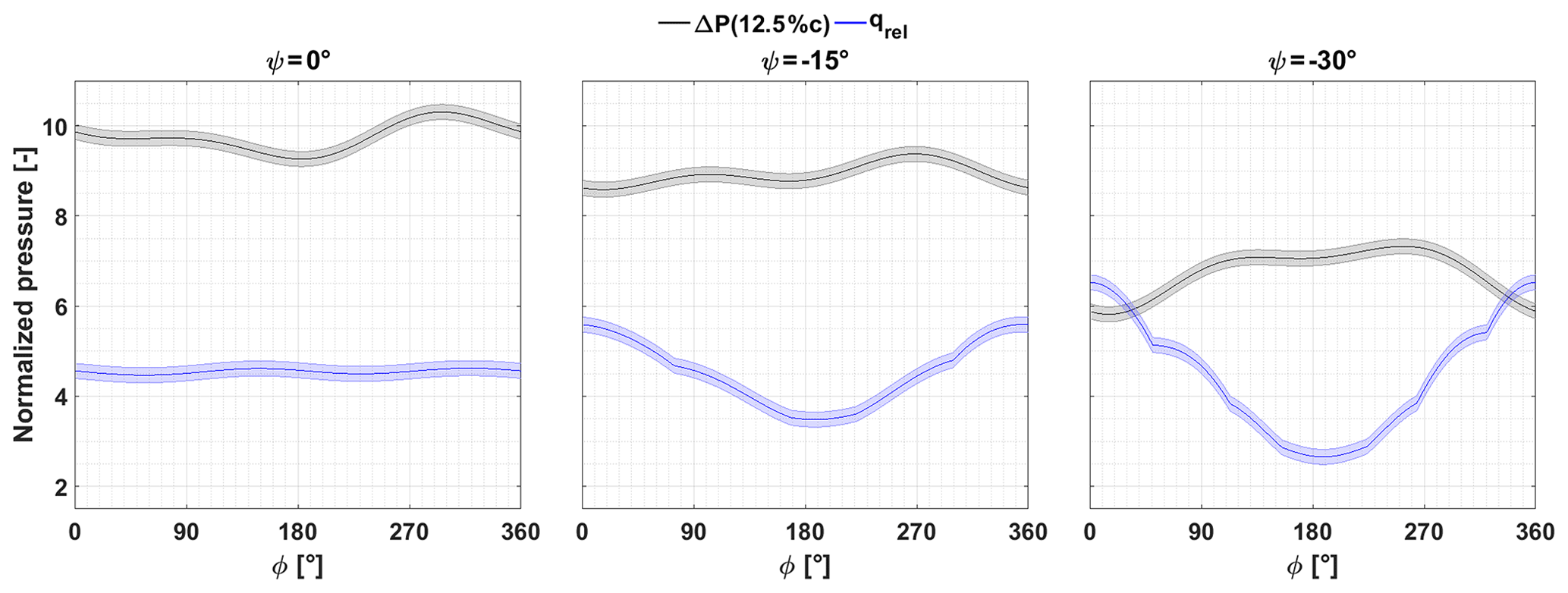
Figure 11Results from pressure taps at r=45%R. For three yaw angles, relative dynamic pressure (qrel) and pressure difference between the pressure and the suction side of the blade at 12.5%c variations with azimuth angle. Values are normalized by the dynamic pressure q∞.
For the aligned case, ψ=0∘, the relative dynamic pressure remains relatively constant at qrel=4.5q∞, while the pressure difference at 12.5%c exhibits four marked behaviors:
Initially, , remaining relatively constant at ΔP(12.5%c)=9.8q∞. Then the dynamic pressure drops, to reach a minimum at ϕ=180∘ (9.3q∞), while an increase follows from ϕ=180∘ to ϕ=290∘. At that point, the dynamic pressure reaches its maximum value (10.3q∞) before it starts dropping to reach 9.8q∞ at ϕ=360∘.
This behavior agrees qualitatively with computational results made by Schulz et al. (2017), where it is shown an asymmetrical axial load, even without the presence of yaw misalignment.
With the introduction of yaw misalignment ∘, the relative dynamic pressure is influenced by the yaw angle, showing a symmetrical trend with its minimum value at an azimuth angle of ϕ=180∘. The maximum variation is . The pressure difference at 12.5%c displays similar features as in the aligned case, but with a shifted azimuth angle position, getting its minimum, ΔP(12.5%c)=8.5q∞, at ϕ=0∘ and its maximum, ΔP(12.5%c)=9.5q∞, at ϕ=270∘. This behavior suggests being related to the advancing and retreating behavior described by Schulz et al. (2017).
For the case of yaw angle ∘, the relative dynamic pressure behavior remains and the drop increases up to Δqrel≈3.8q∞. In the case of the pressure difference at 12.5%c, the azimuth angle dependency becomes more important and the advancing and retreating influence is more pronounced, producing a plateau between azimuth angles .
In terms of the measurement range, the relative pressure is . Over this range, the uncertainty error represents 4.5 %. In the case of the pressure difference at 12.5%c, the range is , where the error takes a value of 4 %.
The magnitude of the dynamic pressure, qrel, and the location of the stagnation point fluctuate along the azimuth position in the misaligned cases. Figure 12 provides an overview of the stagnation point location and the pressure magnitude variation for the different yaw cases in the region close to the leading edge (). The position of the stagnation point at each azimuth angle is indicated on the pressure contours by circles (∘).
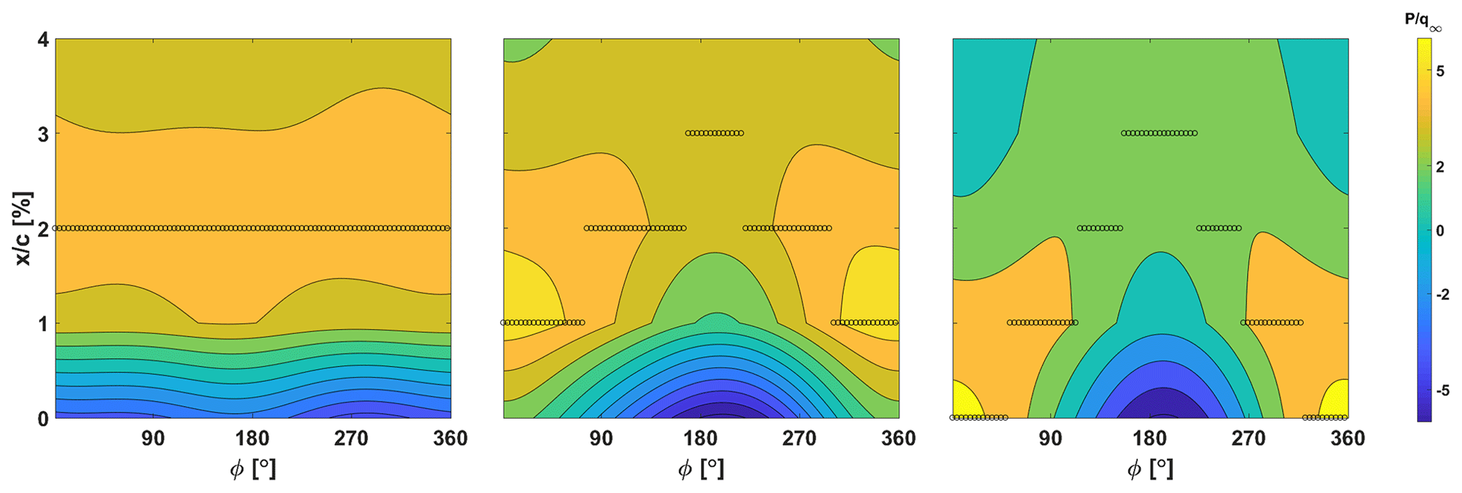
Figure 12Pressure contours over the pressure side at r=45%R in the range [0,4]%c for all yaw cases and pitch angle of θ=0∘. The circles (∘) are located at max{P} at that azimuth position and indicate the location of the stagnation point.
It can be seen that for the case of a yaw angle ψ=0∘, Fig. 12 (left), the relative dynamic pressure position is always at x=2%c. Conversely, for the yaw angle ∘ case, Fig. 12 (middle), the stagnation point is farther upstream (x=1 %) at an azimuth angle ϕ=0∘ and moves downstream towards x=3 % for ϕ=180∘ and back to x=1 % as the blade moves towards the ϕ=0∘ position. Finally, for the case of yaw ∘, Fig. 12 (right), the behavior of the stagnation point is similar, but more pronounced, between x=0 % and x=3 % at azimuth angles of ϕ=0∘ and ϕ=180∘, respectively.
The pressure taps are located at discrete points on the blade surface. For this reason, the sensor that estimates the stagnation point, i.e., the values of the relative dynamic pressure, fluctuates in location. The latter explains the sharp changes present in yaw angle ∘ at azimuth angles ϕ≈70∘ and ϕ≈300∘ and yaw angle ∘ at azimuth angles of ϕ≈50∘ and ϕ≈320∘ (see Fig. 11).
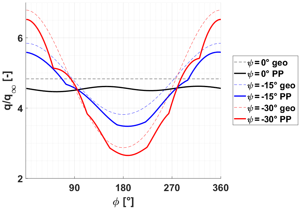
Figure 13Normalized relative dynamic pressure at radial position r=45%R for the yaw cases. The solid line shows the pressure tap estimation. The dashed line shows the geometrical calculation.
Regarding the drop in relative dynamic pressure for the misalignment cases, this can be explained with the geometrical velocities. Equation (10) shows both normal and tangential contributions resulting from the relative dynamic pressure (see Eqs. 7 and 8).
Figure 13 shows the relative dynamic pressure at the radial position r=45%R for the aligned and misalignment cases, normalized by the free-stream dynamic pressure q∞. The same trend between the geometrical case (dashed line) and the estimation from the pressure taps (PP, solid line) as well in the maximum (ϕ=0∘) and minimum (ϕ≈180∘) azimuth positions can be seen.
4.2 Angle-of-attack estimation
4.2.1 Test cases
Figures 14, 15 and 16 show the AoA results from the pressure tap (PP 45%R) and the three-hole-probe (3HP) methods over the three yaw angle cases. In the interest of clarity, only one of the pitch angles is presented here for each yaw angle case. For completeness, the results for the remaining pitch cases can be found in Appendix E, and an analysis through the pitch cases is presented in Sect. 4.2.2.

Figure 14AoA results for yaw angle ψ=0∘ and pitch angle θ=0∘. Pressure taps and three-hole-probe approaches (a). Analytical calculations (b).
Figure 14 shows the AoA for the pressure tap and three-hole-probe approaches (left) and the analytical calculations (right) at a pitch angle θ=0∘ in the aligned case. It can be seen that the two approaches are able to capture the tower influence, which produces a reduction of the AoA around the azimuth angle of ϕ=180∘. However, the AoA from the three-hole-probe method captures a drop near the zone of azimuth angles ϕ≈90∘ and ϕ≈290∘. This behavior has been seen in previous results of Klein et al. (2018), Bartholomay et al. (2018) and Marten et al. (2018).
The explanation is due to the heterogeneity of the inflow. These variations, m s−1 (see Fig. 2), can have the same influence as the tower over the AoA estimations. The geometrical estimation (αgeo) under such inflow variations results in an AoA difference of ∘, which supports this statement.
Although the AoA over the azimuthal variation is not constant, both methods estimate a similar AoA range. The AoAs for both pressure tap and three-hole-probe methods are slightly lower than previous experimental results show by Klein et al. (2018), but within the uncertainty values. Table 3 shows the range (αmin, αmax) and average () values of the AoA over the azimuth angle for the pressure taps and the three-hole-probe methods. The range of the tool measurements is between 6.6–7.8∘, and the geometrical estimation is between 6.4–6.8∘.
On previous work by Klein et al. (2018) and Marten et al. (2018) the AoA estimations made with far-field considerations showed an offset of Δαoff=2.3∘ with respect to the three-hole probes. The smaller difference between experimental and analytical estimations in the current work supports the fact that the blockage model is well implemented.
Additionally, Table 3 shows a comparison between the pressure tap and each three-hole probe. The overall average AoA difference, , shows that there is a small difference between the pressure tap and three-hole-probe methods, up to ∘, whereas the AoA maximum difference, , located around the azimuth angle of ϕ≈300∘ takes the values of Δαmax=1.2∘. However, the difference is of the same magnitude as that of the fluctuations of each tool.
Table 3AoA from the pressure taps and three-hole-probe methods at a yaw angle of ψ=0∘. Average, minimum and maximum for the pitch angle case θ=0∘.
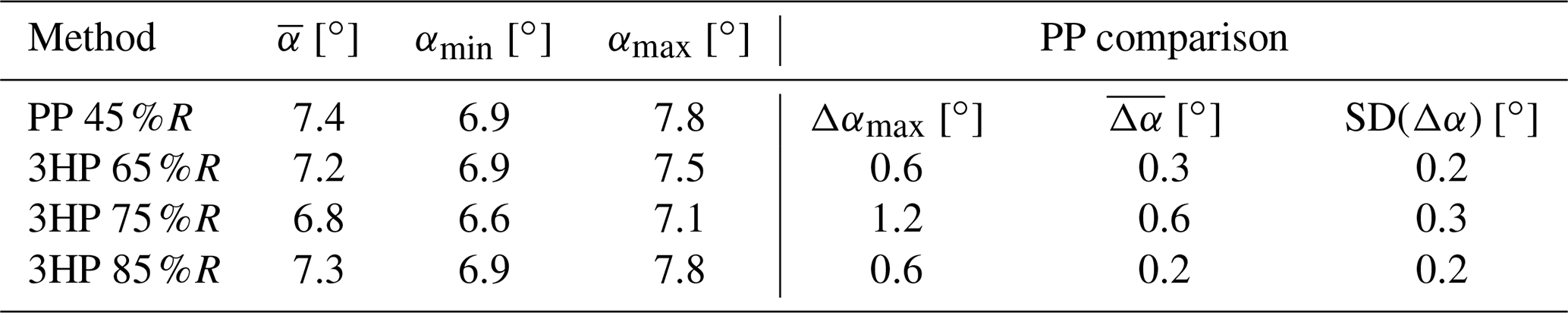
Figure 15 shows the AoA from the pressure tap and three-hole-probe methods (left) and analytical calculations (right) for the pitch angle θ=0∘ and the yaw misalignment of ∘.
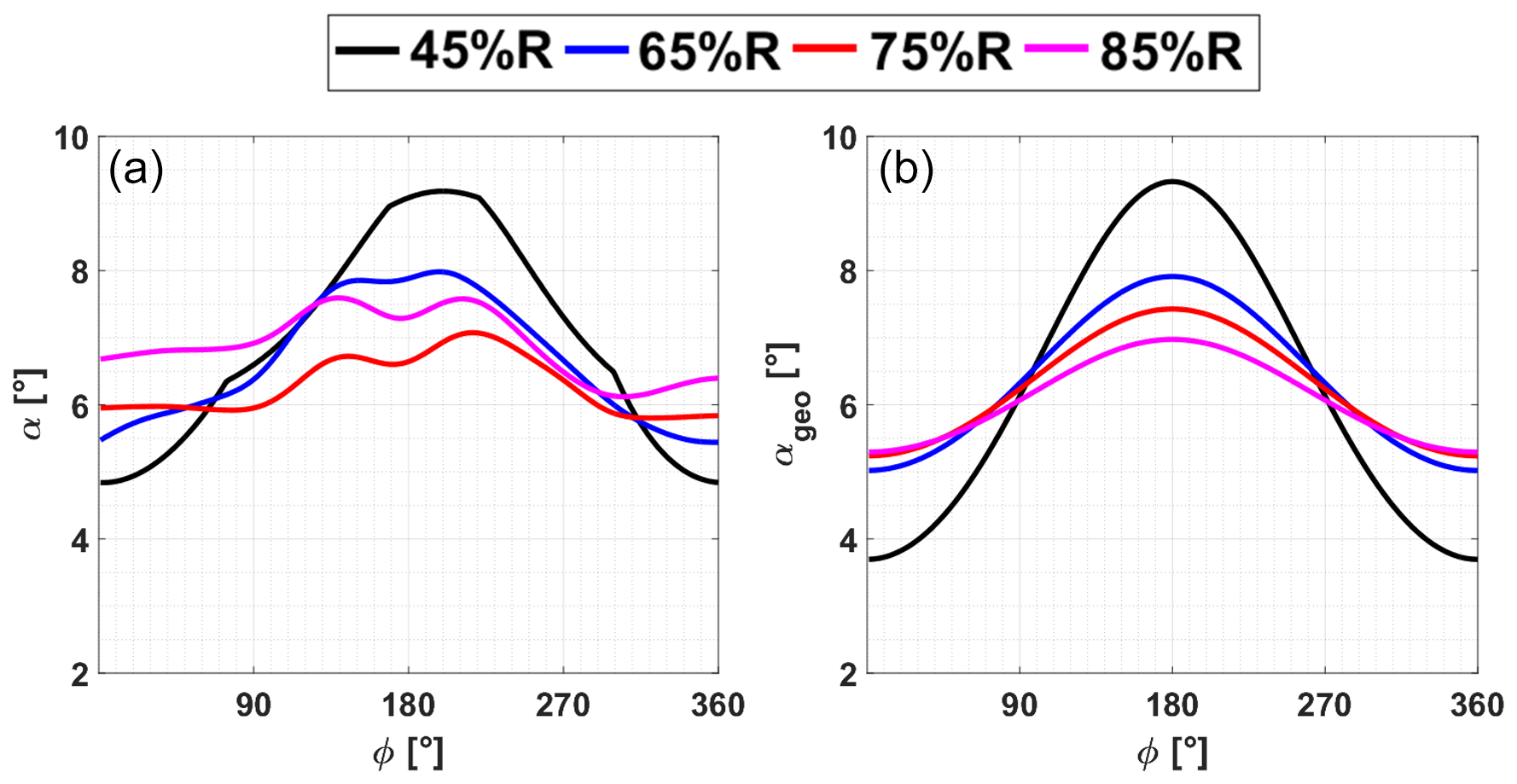
Figure 15AoA results for yaw angle ∘ and pitch angle θ=0∘. Pressure taps and three-hole-probe approaches (a). Analytical calculations (b).
From Fig. 15 (left), it can be noticed that the AoA estimation from the pressure tap starts with smaller values until azimuth angle ∘ where it becomes larger than the AoA from the three-hole-probe estimation. The three-hole-probe approach still shows the tower influence with a drop in the AoA around the azimuth angle ϕ=180∘, in contrast with the pressure tap method, where the AoA keeps increasing until the maximum position located at an azimuth angle of ϕ≈200∘. A reduction in the AoA is followed by the pressure tap estimation becoming smaller than the three-hole-probe approach, as the blade is moving towards the azimuth angle ϕ=0∘.
The same behavior is presented in the case of analytical AoA, Fig. 15 (right) with two main differences. First, there is no tower effect, due to the analytical approach not taking this into consideration. Second, a particular behavior is noticed regarding the three-hole probes at 75 % and 85%R, where their positions are shifted. This could be caused by an error in the mounting, due to it also being visible without misalignment (Fig. 14).
For this yaw misalignment, it is shown that the three-hole probe has a trend less pronounced than the pressure tap approach between ∘ and ∘. Furthermore, the crossflow has partially covered the influence of the tower in the pressure tap method, increasing the AoA disagreement between both methods is in the azimuth angle range ∘.
Figure 16 shows the AoA from the pressure tap and three-hole-probe methods (left) and analytical calculations (right) for the pitch angle θ=0∘ and the yaw misalignment of ∘.
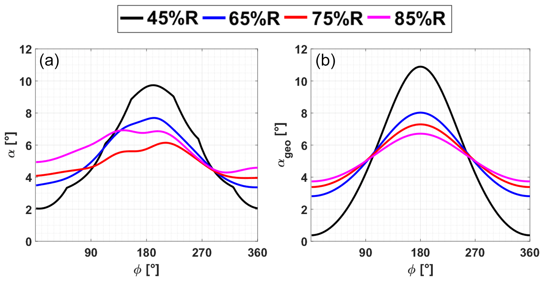
Figure 16AoA results for yaw angle ∘ and pitch angle θ=0∘. Pressure taps and three-hole-probe approaches (a). Analytical calculations (b).
The behavior of the AoA results from the pressure tap method, Fig. 16 (left), in this case, is similar to the yaw angle ∘, exhibiting a more pronounced difference with the three-hole-probe approach at the azimuth angle ϕ=180∘. The effect of the crossflow due to the yaw misalignment is dominant in this case, diminishing the AoA drop around the azimuth angle ϕ=180∘ in the three-hole probe and with a steeper maximum in the case of the pressure tap, in contrast with the previous yaw case.
The analytical AoAs, Fig. 16 (right), show the same features, including the large difference at azimuth angles ϕ=0∘ and ϕ=180∘.
Overall, the pressure tap method presents good results, qualitatively and quantitatively. In the aligned case, the average difference between three-hole probes and analytical AoA is below 1∘. Under yaw misalignments, the pressure tap method in comparison with the analytical method shows an average difference of and for yaw angles of ∘ and ∘, respectively. The larger differences are presented at an azimuth angle of ϕ=0∘.
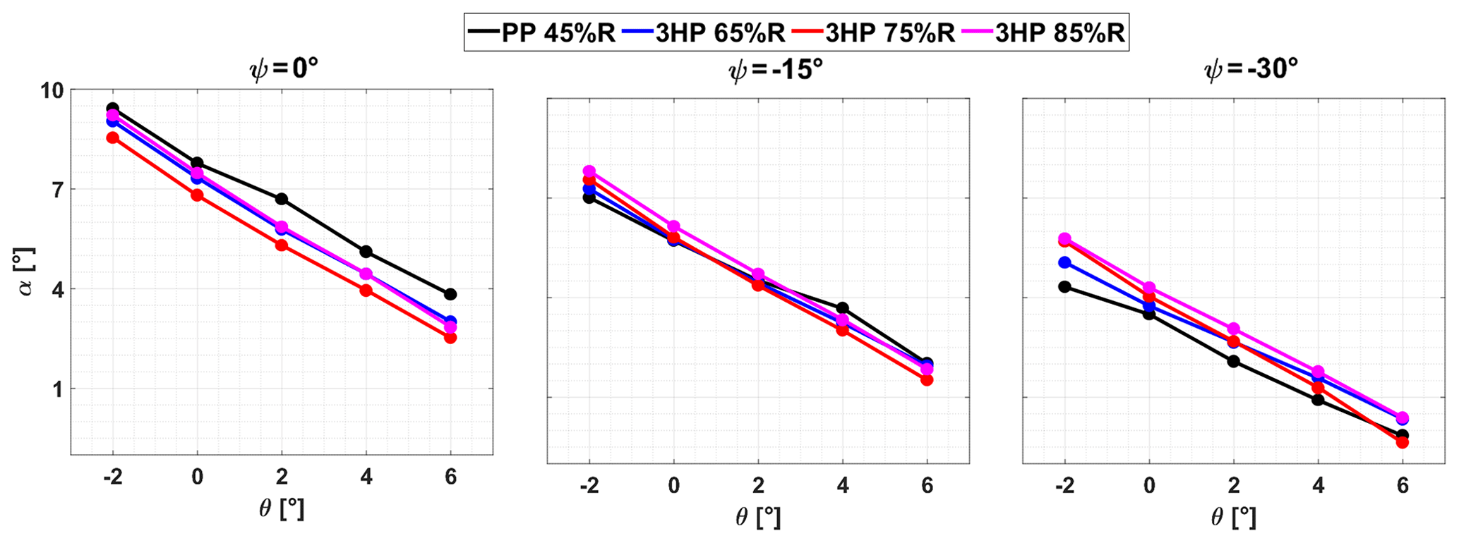
Figure 17AoA estimations from pressure tap and three-hole-probe methods and variations with pitch angle. Three yaw cases ψ=0, −15 and −30∘.
4.2.2 Pitch analysis
A comparison between the AoA estimations from both approaches through the pitch angle cases, at a fixed azimuth position, ϕ=315∘, was analyzed. Figure 17 shows the evolution of AoA estimations at the azimuth angle of ϕ=315∘. It can be observed that the trend is linear for both methods. While the yaw angle increases, the pressure tap method changes from estimating larger to estimating smaller values than three-hole probes.
A linear fit was obtained, in order to check the relation between AoA and pitch angle. The slopes take values around . From the geometrical point of view (see Eq. 9), the expected slope between the AoA and pitch is . Nevertheless, the induction factors change at each pitch angle; therefore the change in the slope is the result of that dependency. This agrees with the fact that the slopes are similar but not the same, as is expected variations of the induction factor along the radial positions are expected.
A method to determine the AoA based on the pressure difference between the pressure and suction side on a wind turbine blade was tested. The method was compared with the AoA results from three three-hole probes in simultaneous wind tunnel measurements together with analytical calculations. Several conditions were studied regarding the introduction of yaw misalignment and different pitch angles for the blades.
The pressure distribution on the blade at 45%R was measured through chordwise pressure taps. The tested method uses the information of a reduced number of pressure taps located close to the blade leading edge in order to estimate the relative dynamic pressure compared to its corresponding blade section. Additionally, the pressure difference between suction and pressure side of the blade at 12.5%c is tracked in order to determine the AoA based on 2-D assumptions.
The application of the method can be summarized as follows.
- 1.
2-D calculations.
- a.
Perform computational calculations or 2-D airfoil measurements to obtain the pressure distribution CP of the same profile to study 3-D.
- b.
Get a fit equation between the pressure difference of the lower and upper sides ΔCP at 12.5%c and AoA: .
- a.
- 2.
3-D estimations.
- a.
Perform pressure distribution measurements at a blade section with similar characteristics of the 2-D airfoil. Only pressure taps at 12.5%c are needed.
- b.
Identify the relative dynamic pressure, qrel, at the azimuth station. The method of the stagnation point was presented here. Pressure taps at the leading edge vicinity would be needed.
- c.
Estimate the AoA through the inverse equation from the 2-D calculations: .
- a.
The main restrictions are the use of a thin airfoil and attached flow.
The results show that in the aligned case, ψ=0∘, the pressure tap approach is suitable, being capable of capturing the same features of the AoA results from the three-hole probes, including the influence of the tower effect. The comparison between the pressure tap method and the three three-hole probes presents a maximum average difference of .
With the introduction of yaw misalignment, the AoA results from the pressure tap method show, as expected, the crossflow influence in a more pronounced curve than the three-hole probe, in agreement with the analytical results. The crossflow impact is more dominant than the tower effects, and the pressure tap method is not able to predict its influence, from where an AoA overestimation in the azimuth region of ∘ can be inferred.
Regarding the pitch angle changes in the blades, the AoA results from the pressure tap approach present a linear behavior with a slope value of , similarly to the three-hole-probe method, being capable of capturing the resulting effects from the axial and tangential induction.
Overall, it is found that the pressure tap method applied here to determine the AoA provides reliable data, with good performance for both aligned and misaligned cases. Hence, the presented method is a promising alternative to the use of external probes, which affect the flow over the blade and require additional calibration.
| α | Angle of attack |
| U | Velocity |
| ψ | Yaw angle |
| ϕ | Azimuth angle |
| λ | Tip speed ratio |
| f | Rated frequency |
| R | Rotor radius |
| γ | Twist angle |
| θ | Pitch angle |
| c | Chord length |
| r∕R | Nondimensional radial blade position [0,1] |
| x | Horizontal chord position |
| x | Nondimensional chordwise coordinate [0,1] |
| y | Vertical chord position |
| X | Axial wind tunnel position |
| Y | Lateral wind tunnel position |
| Z | Vertical wind tunnel position |
| R2 | Coefficient of determination |
| ρ | Air density |
| Ω | Angular velocity |
| q | Dynamic pressure |
| g | Gaunaa model contribution in |
| pressure distribution | |
| β | Flap angle |
| k | Fit constant |
| %R | Radial blade position in percent of rotor radius |
| %c | Horizontal chordwise position in percent of chord length |
| PP | Pressure tap method |
| 3HP | Three-hole-probe method |
| BeRT | Berlin Research Turbine |
| AoA | Angle of attack |
| ∞ | Free stream |
| ref | Reference value |
| upper | Blade section suction side |
| lower | Blade section pressure side |
| s | Sensor |
| corr | Corrected value |
| probe | In reference to probe coordinate system |
| probe, section | In reference to blade section |
| coordinate system | |
| rel | Relative |
| c | Circulatory |
| eff | Effective |
| camb | Camber |
| L | Nonlinear terms |
| t | Tangential |
| n | Normal |
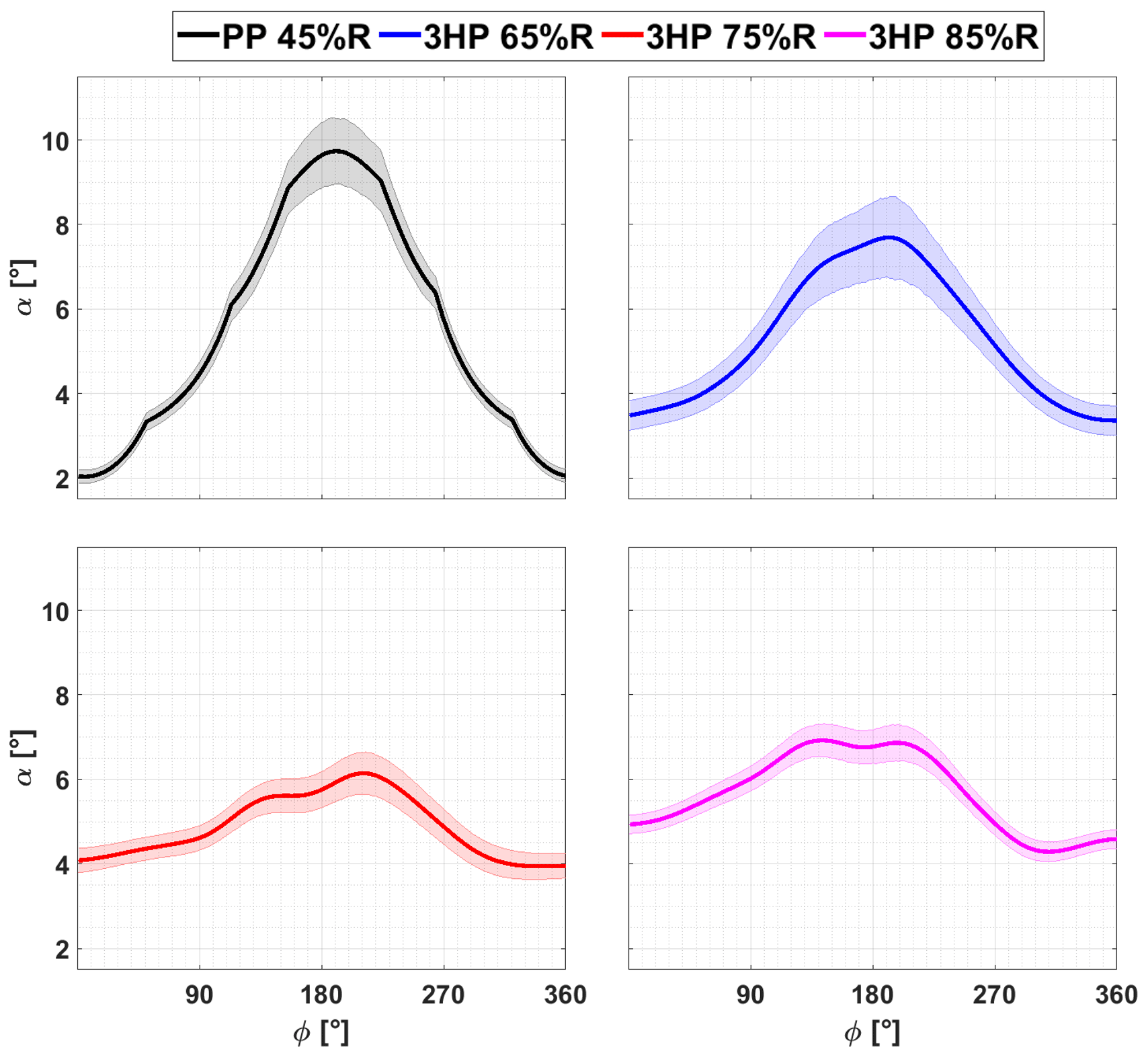
Figure D1AoA results from the pressure tap and three-hole-probe approaches with their uncertainties. The pitch angles θ=0∘ and the yaw angle is ∘.
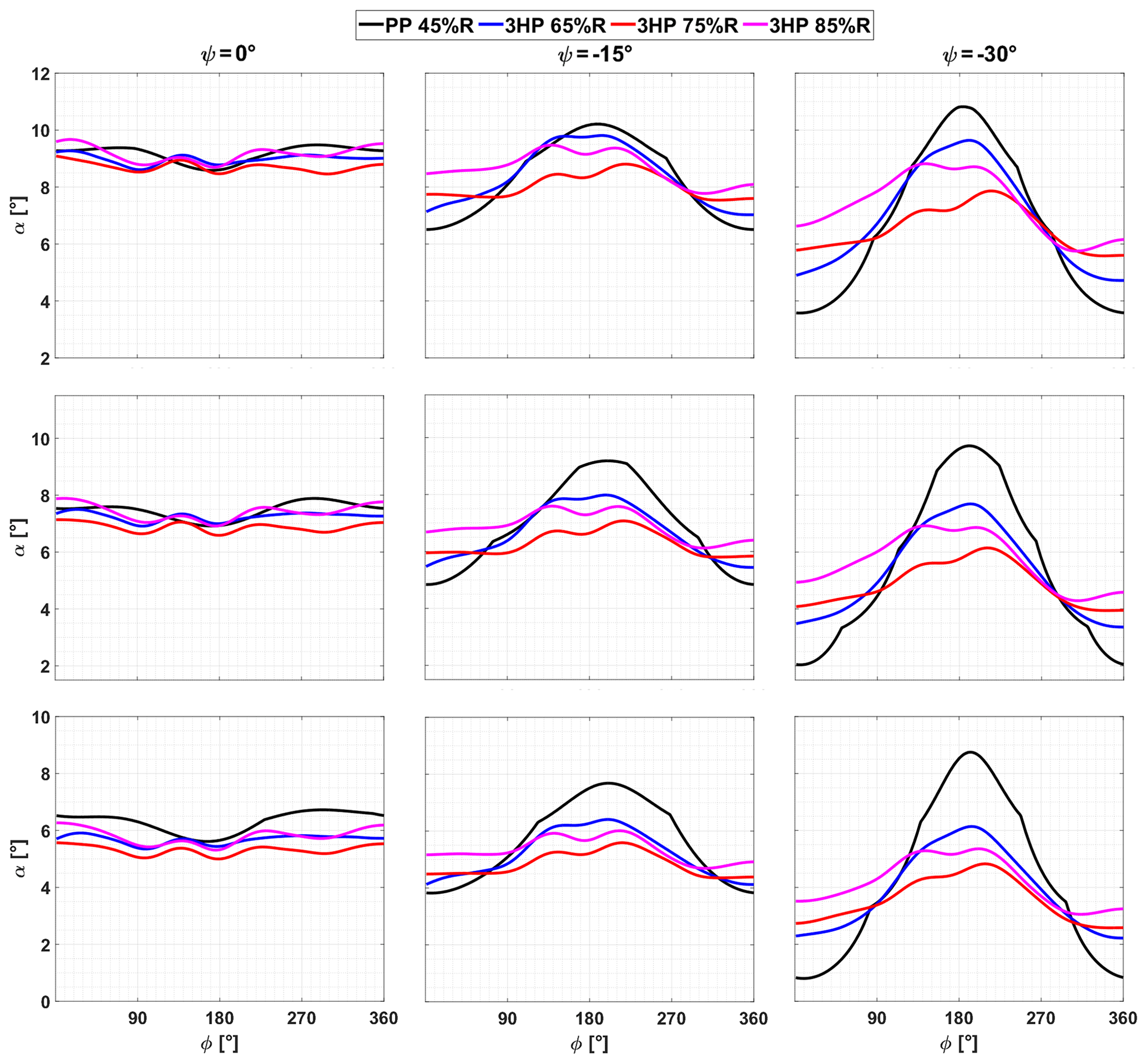
Figure E1AoA results from the pressure tap and three-hole-probe approaches. In columns are shown the yaw angles: ψ=0∘, ∘ and ∘. In rows are shown the pitch angles: ∘, θ=0∘ and θ=2∘.
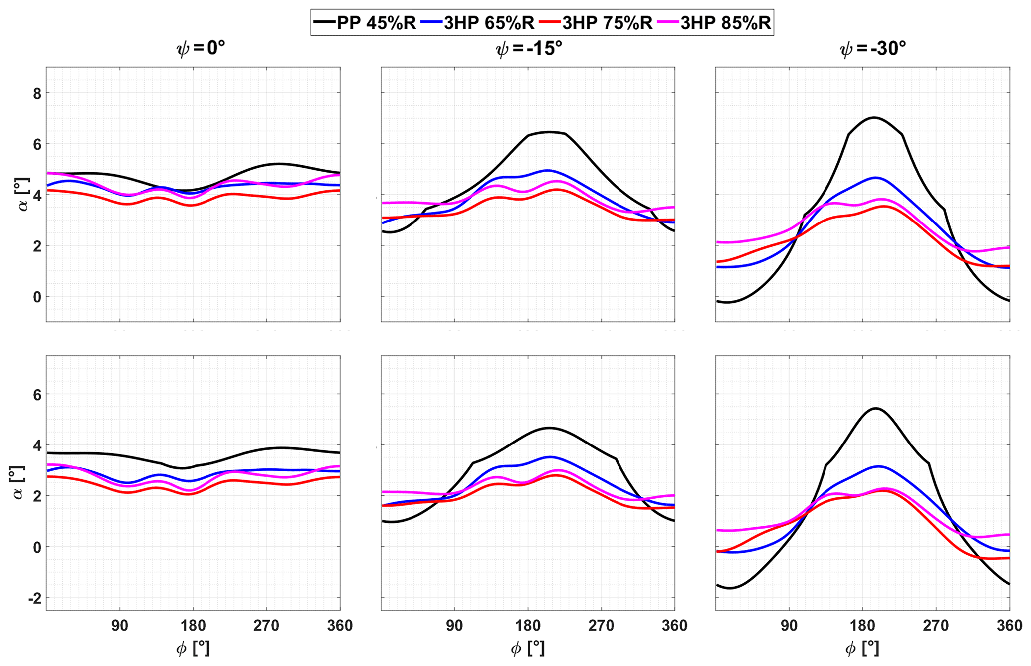
Figure E2AoA results from the pressure tap and three-hole-probe approaches. In columns are shown the yaw angles: ψ=0∘, ∘ and ∘. In rows are shown the pitch angles: θ=4∘ and θ=6∘.
Pressure measurement data and results can be provided by contacting the corresponding author.
RSV carried out the measurement campaign with the support of JA and SB. RSV worked in the implementation of the pressure tap method, performed the calculations and analysis, and wrote the paper. SB provided the code for the three-hole-probe method. JA, SB, MM, CNN and COP contributed with comments and discussions about each section in the manuscript.
The authors declare that they have no conflict of interest.
This article is part of the special issue “Wind Energy Science Conference 2019”. It is a result of the Wind Energy Science Conference 2019, Cork, Ireland, 17–20 June 2019.
The authors would like to acknowledge Joseph Saverin for providing valuable feedback.
This research has been supported by the ANID PFCHA/Becas Chile-DAAD/2016 (grant no. 91645539).
This open-access publication was funded
by Technische Universität Berlin.
This paper was edited by Katherine Dykes and reviewed by Uwe Paulsen and one anonymous referee.
Bak, C., Troldborg, N., and Madsen, H. A.: DAN-AERO MW: Measured airfoil characteristics for a MW rotor in atmospheric conditions, in: EWEA Annual Event 2011, European Wind Energy Association (EWEA), Brussels, Belgium, 14–17 March 2011. a, b, c
Bartholomay, S., Fruck, W.-L., Pechlivanoglou, G., Nayeri, C. N., and Paschereit, C. O.: Reproducible Inflow Modifications for a Wind Tunnel Mounted Research Hawt, in: ASME Turbo Expo 2017: Turbomachinery Technical Conference and Exposition, Charlotte, North Carolina, USA, 26–30 June 2017, American Society of Mechanical Engineers, GT2017-64364, V009T49A013, 12 pp., 2017. a, b, c
Bartholomay, S., Michos, G., Perez-Becker, S., Pechlivanoglou, G., Nayeri, C., Nikolaouk, G., and Paschereit, C. O.: Towards Active Flow Control on a Research Scale Wind Turbine Using PID controlled Trailing Edge Flaps, in: Wind Energy Symposium, Kissimmee, Florida, 8–12 January 2018, AIAA 2018-1245, 17 pp., https://doi.org/10.2514/6.2018-1245, 2018. a, b
Bechmann, A., Sørensen, N. N., and Zahle, F.: CFD simulations of the MEXICO rotor, Wind Energy, 14, 677–689, 2011. a
Bergh, H. and Tijdeman, H.: Theoretical and experimental results for the dynamic response of pressure measuring systems, Nationaal Lucht- en Ruimtevaartlaboratorium, Tech. Rep. NLR-TR F.238, 1965. a, b, c
Brand, A., Schepers, J., Dekker, J., de Groot, C., Ramakers, S., M., S., and van der Burg, N.: ECN Field Rotor-Aerodynamics: Past, present and future, in: IEA Joint Action, 11th IEA Symposium on the Aerodynamics of Wind Turbines, Petten, the Netherlands, 18–19 December 1997, pp. 3–33, 1997. a, b
Brand, A. J.: To estimate the angle of attack of an airfoil from the pressure distribution, ECN Wind Energy, 1994. a
Bruining, A. and van Rooij, R.: Two- and three-dimensional aerodynamic performance of the NLF(1)0416 airfoil on a wind turbine blade, in: IEA Joint Action, 11th IEA Symposium on the Aerodynamics of Wind Turbines, , 59–76, 1997. a, b, c, d
Corten, G. P.: Flow separation on wind turbines blades, PhD thesis, Universiteit Utrecht, Nederland, 2001. a
Drela, M. and Youngren, H.: XFOIL; Subsonic Airfoil Development System, Massachusetts Institute of Technology, Massachusetts, USA, available at: https://web.mit.edu/drela/Public/web/xfoil/ (last access: February 2020), 2001. a
Dudzinski, T. J. and Krause, L. N.: Flow-direction measurement with fixed-position probes, NASA, Lewis Research Center, USA, Tech. rep., NASA TM X-1904, 1969. a
Gallant, T. and Johnson, D.: In-blade angle of attack measurement and comparison with models, J. Phys. Conf. Ser., 753, 072007, https://doi.org/10.1088/1742-6596/753/7/072007, 2016. a
Gaunaa, M.: Unsteady aerodynamic forces on NACA 0015 airfoil in harmonic translatory motion, Technical University of Denmark, MEK-FM-PHD, PhD thesis, 2002. a, b
Gaunaa, M.: Unsteady 2D potential-flow forces on a thin variable geometryairfoil undergoing arbitrary motion, Forskningscenter Risoe, Denmark, Tech. Rep., Risø-R, No. 1478(EN), 2006. a, b, c, d
Gaunaa, M. and Andersen, P. B.: Load reduction using pressure difference on airfoil for control of trailing edge flaps, in: 2009 European Wind Energy Conference and Exhibition, Marseille, France, 16–19 March 2009, EWEC, 2009. a, b, c, d, e, f, g
Glauert, H.: The Elements of Aerofoil and Airscrew Theory, Cambridge University Press, ISBN: 9780511574481, https://doi.org/10.1017/CBO9780511574481, 1926. a
Guntur, S. and Sørensen, N. N.: An evaluation of several methods of determining the local angle of attack on wind turbine blades, Journal of Physics: Conference Series, 555, 012045, https://doi.org/10.1088/1742-6596/555/1/012045, 2012. a
Hand, M., Simms, D., Fingersh, L., Jager, D., Cotrell, J., Schreck, S., and Larwood, S.: Unsteady aerodynamics experiment phase VI: wind tunnel test configurations and available data campaigns, Tech. rep., No. NREL/TP-500-29955, National Renewable Energy Laboratory (NREL), Golden, CO, US, 2001. a, b
Klein, A. C., Bartholomay, S., Marten, D., Lutz, T., Pechlivanoglou, G., Nayeri, C. N., Paschereit, C. O., and Krämer, E.: About the suitability of different numerical methods to reproduce model wind turbine measurements in a wind tunnel with a high blockage ratio, Wind Energ. Sci., 3, 439–460, https://doi.org/10.5194/wes-3-439-2018, 2018. a, b, c, d, e, f, g, h, i, j
Madsen, H. A., Petersen, J. T., Bruining, A., Brand, A., and Graham, M.: Field rotor measurements. Data sets prepared for analysis of stall hysteresis, Risoe-R, No. 1046(EN), 1998. a, b
Maeda, T., Ismaili, E., Kawabuchi, H., and Kamada, Y.: Surface pressure distribution on a blade of a 10 m diameter hawt (field measurements versus wind tunnel measurements), J. Sol. Energy Eng., 127, 185–191, 2005. a, b, c
Marten, D., Lennie, M., Pechlivanoglou, G., Nayeri, C. N., and Paschereit, C. O.: Implementation, optimization and validation of a nonlinear lifting line free vortex wake module within the wind turbine simulation code QBlade, in: ASME Turbo Expo 2015: Turbine Technical Conference and Exposition, American Society of Mechanical Engineers Digital Collection, Montreal, Quebec, Canada, 15–19 June 2015. a
Marten, D., Bartholomay, S., Pechlivanoglou, G., Nayeri, C., Paschereit, C. O., Fischer, A., and Lutz, T.: Numerical and Experimental Investigation of Trailing Edge Flap Performance on a Model Wind Turbine, in: 2018 Wind Energy Symposium,Kissimmee, Florida, 8–12 January 2018, p. 1246, 2018. a, b
Marten, D., Paschereit, C. O., Huang, X., Meinke, M. H., Schroeder, W., Mueller, J., and Oberleithner, K.: Predicting Wind Turbine Wake Breakdown Using a Free Vortex Wake Code, in: AIAA Scitech 2019 Forum, San Diego, California, 7–11 January 2019, AIAA 2019-2080, p. 2080, https://doi.org/10.2514/6.2019-2080, 2019. a
Morote, J.: Angle of attack distribution on wind turbines in yawed flow, Wind Energy, 19, 681–702, 2016. a
Moscardi, A. and Johnson, D. A.: A compact in-blade five hole pressure probe for local inflow study on a horizontal axis wind turbine, Wind Engineering, 40, 360–378, 2016. a, b, c
Pechlivanoglou, G., Fischer, J., Eisele, O., Vey, S., Nayeri, C., and Paschereit, C.: Development of a medium scale research hawt for inflow and aerodynamic research in the tu berlin wind tunnel, in: 12th German Wind Energy Conference (DEWEK), Bremen, Germany, 19–20 May 2015. a, b
Refan, M. and Hangan, H.: Aerodynamic performance of a small horizontal axis wind turbine, J. Sol. Energy Eng., 134, 021013, https://doi.org/10.1115/1.4005751, 2012. a
Ronsten, G.: Static pressure measurements on a rotating and a non-rotating 2.375 m wind turbine blade. Comparison with 2D calculations, Wind. Eng. Ind. Aerod., 39, 105–118, 1992. a, b
Sant, T., van Kuik, G., and van Bussel, G. J. W.: Estimating the angle of attack from blade pressure measurements on the NREL phase VI rotor using a free wake vortex model: axial conditions, Wind Energy, 9, 549–577, 2006a. a
Sant, T., van Kuik, G., and van Bussel, G.: Estimating the Unsteady Angle of Attack from Blade Pressure Measurments on the NREL Phase VI Rotor in Yaw using a Free-Wake Vortex Model, in: 44th AIAA Aerospace Sciences Meeting and Exhibit, Reno, Nevada, 9–12 January 2006, AIAA 2006-393, p. 393, https://doi.org/10.2514/6.2006-393, 2006b. a
Sant, T., van Kuik, G., and Van Bussel, G.: Estimating the angle of attack from blade pressure measurements on the National Renewable Energy Laboratory phase VI rotor using a free wake vortex model: yawed conditions, Wind Energy, 12, 1–32, 2009. a
Schepers, J. and Schreck, S.: Aerodynamic measurements on wind turbines, WIREs Energy Environ., 8, e320, https://doi.org/10.1002/wene.320, 2019. a
Schepers, J. and Van Rooij, R.: Final report of the Annexlyse project: Analysis of aerodynamic field measurements on wind turbines, Energy research Centre of the Netherlands (ECN), Petten, Netherlands, Technical Report, ECN-C-05-064, 49 pp., 2005. a
Schepers, J., Brand, A., Bruining, A., Graham, J., Hand, M., Infield, D., Madsen, H., Paynter, R., and Simms, D.: Final report of IEA Annex XIV: field rotor aerodynamics, Energy research Centre of the Netherlands (ECN), Petten, Netherlands, Technical Report, ECN-C-97-027, 1997. a
Schepers, J., Brand, A., Bruining, A., Hand, M., Infield, D., Madsen, H., Maeda, T., Paynter, J., van Rooij, R., Shimizu, Y., Simms, D., Graham, M., and Stefanatos, N.: Final report of IEA Annex XVIII: enhanced field rotor aerodynamics database, Energy research Centre of the Netherlands (ECN), Petten, Netherlands, Technical Report, ECN-C-02-016, 2002. a, b, c, d
Schepers, J., Boorsma, K., Cho, T., Gomez-Iradi, S., Schaffarczyk, P., Jeromin, A., Shen, W. Z., Lutz, T., Meister, K., Stoevesandt, B., Schreck, B., Micallef, D., Pereira, R., Sant, T., Madsen, H. A., and Soerensen, N.: Analysis of Mexico wind tunnel measurements: Final report of IEA Task 29, Mexnext (Phase 1), ECN Wind Energy, Tech. rep., ECN-E–12-004, 291 pp., 2012. a, b
Schepers, J., Lutz, T., Boorsma, K., Gomez-Iradi, S., Herraez, I., Oggiano, L., Rahimi, H., Schaffarczyk, P., Pirrung, G., Madsen, H. A., Shen, W. Z., Rahimi, H., and Schaffarczyk, P.: Final Report of IEA Wind Task 29 Mexnext (Phase 3), ECN Wind Energy, Tech. rep., ECN-E–18-003, 324 pp., 2018. a
Schmid, M.: A fiber-optic sensor for measuring quasi-static and unsteady pressure on wind energy converters, in: 4SMARTS-Symposium für Smarte Strukturen und Systeme, Braunschweig, Germany, 22 June 2017. a
Schulz, C., Letzgus, P., Lutz, T., and Krämer, E.: CFD study on the impact of yawed inflow on loads, power and near wake of a generic wind turbine, Wind Energy, 20, 253–268, 2017. a, b
Shen, W. Z., Hansen, M. O., and Sørensen, J. N.: Determination of the angle of attack on rotor blades, Wind Energy, 12, 91–98, 2009. a
Shipley, D. E., Miller, M. S., Robinson, M. C., Luttges, M. W., and Simms, D. A.: Techniques for the determination of local dynamic pressure and angle of attack on a horizontal axis wind turbine, Tech. rep., NREL/TP-442-7393, National Renewable Energy Laboratory (NREL), Golden, CO, US, 1995. a, b
Sicot, C., Devinant, P., Loyer, S., and Hureau, J.: Rotational and turbulence effects on a wind turbine blade. Investigation of the stall mechanisms, J. Wind. Eng. Ind. Aerod., 96, 1320–1331, 2008. a
Simms, D. A., Hand, M., Fingersh, L., and Jager, D.: Unsteady aerodynamics experiment phases II-IV test configurations and available data campaigns, National Renewable Energy Laboratory (NREL), Golden, CO, US, Technical Report, NREL/TP-500-25950, 177 pp., 1999. a, b
Tsilingiris, P.: Thermophysical and transport properties of humid air at temperature range between 0 and 100 C, Energ. Convers. Manage., 49, 1098–1110, 2008. a
Velte, C. M., Mikkelsen, R. F., Sørensen, J. N., Kaloyanov, T., and Gaunaa, M.: Closed loop control of a flap exposed to harmonic aerodynamic actuation, in: The science of Making Torque from Wind 2012: 4th scientific conference, Oldenburg, Germany, 9–11 October 2012. a, b
Vey, S., Marten, D., Pechlivanoglou, G., Nayeri, C., and Paschereit, C. O.: Experimental and numerical investigations of a small research wind turbine, in: 33rd AIAA Applied Aerodynamics Conference, 22–26 June 2015, Dallas, TX, AIAA 2015-3392, https://doi.org/10.2514/6.2015-3392, 2015. a, b
Whale, J., Fisichella, C., and Selig, M.: Correcting inflow measurements from Hawts using a lifting-surface code, in: 37th Aerospace Sciences Meeting and Exhibit, 11–14 January 1999, Reno, NV, U.S.A., AIAA-99-0040, p. 40, https://doi.org/10.2514/6.1999-40, 1999. a, b
Zilliac, G.: Modelling, calibration, and error analysis of seven-hole pressure probes, Exp. Fluids, 14, 104–120, 1993. a
- Abstract
- Introduction
- Experimental setup
- Methodology
- Results and discussion
- Conclusions
- Appendix A: List of symbols
- Appendix B: Abbreviations
- Appendix C: Subscripts
- Appendix D: Uncertainty of the angles of attack
- Appendix E: Angles of attack
- Data availability
- Author contributions
- Competing interests
- Special issue statement
- Acknowledgements
- Financial support
- Review statement
- References