WESgraph: a graph database for the wind farm domain

The construction and management of a wind farm involve many disciplines. It is hard for a single designer or developer to keep an overview of all the relevant concepts, models, and tools. Nevertheless, this is needed when performing integrated modeling or analysis. To help researchers keep this overview, we have created WESgraph (the Wind Energy System graph), a knowledge base for the wind farm domain, implemented as a graph database. It currently contains 1222 concepts and 1725 relations between them. This paper presents the structure of this graph database – content stored in nodes and the relationships between them – as a foundational ontology, which classifies the domain's concepts. This foundational ontology partitions the domain in two: a part describing physical aspects and a part describing mathematical and computational aspects. This paper also discusses a number of generally difficult cases that exist when adding content to such a knowledge base. This paper furthermore discusses the potential applications of WESgraph and illustrates its use for computation pathway discovery – the application that triggered its creation. It also contains a description of our practical experience with its design and use as well as our thoughts about the community use and management of this tool.

1 Introduction

An offshore wind farm is a complex system composed of many subsystems that interact with other subsystems and external systems. Its design involves multiple disciplines, such as installation, operation, maintenance, and decommissioning. The result is that keeping an overview of the wind farm “domain” is hard to do for a single person or a small team. However, at the current stage of development of the domain, during which subsystems such as turbines have already seen a good number of optimized design iterations, the system interactions have become relatively more important. This prompts a more holistic, systems engineering approach to open up the possibility of further gains in, e.g., productivity, efficiency, and robustness (van Kuik et al., 2016). Therefore, a tool that enables a developer, designer, or researcher in the field to keep the overview can provide great benefits.

This paper presents such a tool, WESgraph (Wind Energy System graph). It is a graph database for the wind farm domain. Graph databases are used as knowledge bases for various purposes in diverse domains, such as general human knowledge (Bollacker et al., 2008; Vrandečić and Krötzsch, 2014; Speer et al., 2017), biochemistry and biomedicine (Jupe et al., 2012; Franceschini et al., 2013; Himmelstein and Baranzini, 2015), and aerospace (Taymaz et al., 2013). The envisioned tool shares with these examples from the literature the requirement that it must function as a curated knowledge base for a specific domain. It differs because next to providing a description of the (physical) domain itself, it must also contain descriptions of mathematical models (and computational tools) used within the domain to enable use cases involving these. This difference, together with the inherent ones between scientific domains, means existing knowledge base systems such as the ones referenced above cannot be adapted, although they do function as inspiration. Consequently, WESgraph was essentially built from the ground up by the authors. To the knowledge of the authors, it is the first proposal of its kind in the wind energy field.

Figure 1 Visualization of an excerpt of the content in WESgraph.

In WESgraph, the domain, both in its physical and mathematical aspects, is described using information-carrying nodes (concepts) connected by edges (relationships). Information can be added locally and through the graph structure be connected to the global whole. The database can be queried to return the information desired in the format required.

The creation of this graph database was started in the context of projects dealing with offshore wind farms as a whole. (As a consequence, the reader may notice a focus on offshore farms in the examples.) This includes (i) mapping uncertainty and its propagation through the wind energy system and (ii) exploring the effect of model fidelity on wind farm simulation. However, its usefulness as a tool for multiple purposes soon became apparent, which resulted in its more informed and serious development. It currently contains 1222 concepts and 1725 relations between them, representing a substantial time investment.

Other tools that enable practitioners in the field to keep the overview may be conceived. They could be quite different from WESgraph; consider, for example, a domain-specific collaborative wiki, which has important implications for the possible use cases it enables. So WESgraph should effectively be seen as a proposal. This paper gives a thorough description of WESgraph, brings to the fore its qualities and limitations, and provides reflection. It does not provide an analysis of effectivity, as its use as of yet has been too limited for that. It does provide a very concrete starting point for further exploration, test cases, and discussion in the community.

The paper has two main parts: a general overview of WESgraph and a detailed description. The general overview in Sect. 2 presents the essentials of WESgraph's structure, its content, its content representation challenges, and the use cases considered. Reading this part makes it clear what WESgraph is, why it is valuable, in what ways its construction is nontrivial, and how it can be used. The detailed description in Sect. 3 provides illustrations of many aspects of WESgraph, motivates and contextualizes choices made, makes content addition and usage more concrete, and collects various pertinent thoughts. Its structure parallels the one for the general overview. It enables the interested reader to get a complete, contextualized view of WESgraph and is recommended in case one wishes to contribute to WESgraph. It can also be sampled piecemeal when one is interested in a number of select topics only. After these two main parts, Sect. 4 closes the paper with our conclusions about WESgraph and a vision for its future.

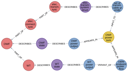
To close this Introduction, Fig. 1 gives a first impression of WESgraph. When using a graph database, it is natural to visualize its content by showing excerpts from the graph. (The whole graph is too large in terms of nodes and edges to be usefully shown in its entirety.) The amenability to such visualizations actually greatly contributes to the usability of the database. This paper makes extensive use of graph visualizations. (The meaning of the different elements of this visualization is discussed later in the paper.) As an example, Fig. 1 shows the relationship between the power output of an offshore wind farm (OWF) and its constituent wind turbines (WTs). The involvement of the electrical connection system (elec. connect. syst.) appears through the transmission cables and the cable endpoints through which the power flows.

2 General overview

To make the content of the database accessible, it should be effectively structured. So this first main part of the paper starts with Sect. 2.1, which describes how the content is structured. Once this structure is in place, content can be added and queried in an informed way. However, the agreed-upon structure does not prescribe how content must be added, which means that representation challenges arise for some parts of the domain. So Sect. 2.2 gives a view of the database's current content and highlights the challenges encountered. The database can be queried in different ways, so to also give an idea about the possible uses, Sect. 2.3 discusses a number of use cases: computational pathway discovery, tool interoperability, defining disciplines, and education.

2.1 The graph database structure of WESgraph

This section discusses the structure of WESgraph. Section 2.1.1 describes the basics: the general concept of a graph database and how its features are used to tailor it specifically to WESgraph's needs. Section 2.1.2–2.1.4 then discuss these specifics. Section 2.1.5 finally briefly touches on WESgraph's practical implementation.

2.1.1 Structuring content in a labeled property graph

A graph database is built on the concept of a graph, which has proven to be a useful way of structuring information. A graph consists of nodes, also called vertices, connected by edges. In Fig. 1, disks represent nodes and arrows between nodes represent edges. WESgraph is a directed graph, as all edges point from one node to a (distinct) second node.

Content is stored in the database as properties, or key-value pairs, attached to nodes and edges. Moreover, a finite number of labels can be attached to nodes and every relationship must have a relationship type. A graph database with such features is called a labeled property graph. In Fig. 1, relationship types (in capital letters) are overlaid on the edges, node labels determine the color coding of nodes, and the value of the property “name” is, to the degree possible given the available space, printed on the node disks.

The features mentioned above provide enormous flexibility in creating the graph structure and adding content. In fact, without restrictions on how content is added and structured, collaboration on adding material to the database and the useful extraction of data is next to impossible because the user would not be able to rely on a known structure. The remainder of this section therefore describes the rules put in place to make consistent use of WESgraph possible. These rules, also called the database schema, are specified using

1. a foundational ontology for the domain, which defines inextricably linked sets of node categories (implemented as labels) and relationship types, and

2. an enumeration of the properties that can or should be attached to nodes and relationships.

The reference diagram in Fig. 2 provides a schematic overview of the categories and relationships defined by the foundational ontology. It also mentions the properties that can be attached to nodes and relationships.

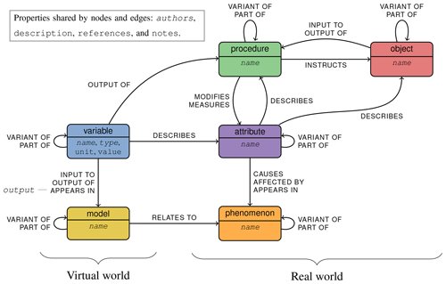
Figure 2 A schematic overview of the categories, relationships, and (required) properties defined by the database schema.

Below, the subsections discuss each of the concepts mentioned above that appear in Fig. 2. Section 2.1.2 describes the categories of WESgraph's foundational ontology, Sect. 2.1.3 describes its relationships, and Sect. 2.1.4 describes the properties.

2.1.2 Categories

When describing a domain, such as wind energy systems, its concepts can be categorized. Such a categorization is the basis for the foundational ontology. Two overarching classes, dubbed the virtual world and the real world, provide a first division. Each of these two classes consists of a number of mutually exclusive categories. For the virtual world, these are

• models, encompassing both mathematical models and computational tools, and

• variables, covering the variables, parameters, and constants used as inputs and outputs for the models.

For the real world, these are

• objects, representing all physical things,

• procedures, describing concrete implementations of planned processes,

• attributes, specifying objects and procedures, and

• phenomena, describing physical processes.

Table 1 gives illustrative examples for each of the categories. In the graph database, labels are used to encode categories.

Table 1 Example concepts for each of the categories defined.

^a Models are often named after the variable they are meant to compute. ^b Variables often have the same name as the attribute they describe.

As already mentioned, in Fig. 1 colors correspond to labels, and therefore colors correspond to categories; from left to right we can see objects (red), attributes (purple), variables (blue), and models (yellow). Figure 2 shows the categories as the nodes of the diagram, with virtual-world categories on the left and real-world categories on the right. Figure 2 shares its color coding with Fig. 1 and other graph extracts.

2.1.3 Relationships

Next to the restriction of nodes to certain categories, the foundational ontology also constrains the relationships between nodes, in a category-dependent manner. For example, from their description above, attributes clearly have a special relationship with members of other categories – objects and procedures. But this is just the tip of the iceberg. All defined relationships are included in the diagram in Fig. 2. Their names are attached to the arrow connecting the categories between which the relationships are defined. The lists below describe their use. Examples and illustrations can be found in the detailed description (Sect. 3.1.3).

There are two intra-category relationships that can be used for all categories:

• is a part of, to decompose concepts into subconcepts, and

• is a variant of, to list more specific variants of a concept.

All the other relationships are inter-category ones. They are also specific to the actual categories of the nodes they connect, although names are reused for similar relationships, for example describes in Fig. 2.

In the virtual world, the inter-category relationships between models and variables express which variables appear in which models and what their role is:

• a variable is an input to a model and cannot be an output,

• a variable is an output of a model and cannot be an input, and

• a variable appears in a model to express that it can be both input and output, depending on the use case of the model.

Attributes form the main connection between the real-world categories object and procedure and the virtual-world category variable. A single relationship name, describes, is used for all the relationships between these categories. Namely,

• a variable describes an attribute, and

• an attribute describes an object or procedure.

Procedures effect change in the real world. To describe how this is done, a number of procedures-specific relationships have been defined. Shared for all procedures is that

• a procedure instructs an object (a crew, for example).

This object performs tasks prescribed by the procedure. Depending on the kind of task, specific relationships are used.

• For changes to which objects are present in the wind energy system, we have

  • objects as input to a procedure and

  • objects as output of a procedure.

• For changes to attributes, we have that

  • a procedure modifies an attribute.

• For measuring attributes, we have that

  • a procedure measures attributes and

  • variables as output of a procedure.

  This relationship between variables and procedures represents the only actual relation between the real world and the virtual world. It represents that measurements and observations in the real world produce data that are used as input to the models.

The last set of relationships are connected to phenomena. As can be seen in Fig. 2, phenomena and attributes mirror models and variables in terms of relationships. Namely,

• an attribute causes a phenomenon but is not itself affected by it,

• an attribute is affected by a phenomenon, but not a cause, and

• an attribute appears in a phenomenon to express that it can be both a cause and effect.

A direct connection with the virtual world can also be made:

• a model relates to a phenomenon.

2.1.4 Properties

Properties provide the means to add actual content to the database. They can be attached to both nodes and edges and form their metadata. All defined properties are mentioned in Fig. 2: in the nodes for category-specific ones, attached to the relationship name it clarifies, or in a separate box for those shared by categories and relationships. To facilitate manageability and discoverability, only properties from a predefined set are allowed. Moreover, some properties must be present on all relationships, all node categories, or specific node categories.

The properties allowed on all nodes and relationships are the following:

• authors (list of strings), listing the email addresses of the people that have added or modified that element in the database, to provide a contact for clarification;

• description (string), containing a description of the concept or a clarification of the relationship in one or a few sentences;

• references (list of strings), containing one or more references to the literature wherein more information about the concept or relationship can be found; and

• notes (list of strings), providing information about recognized issues with how the element fits into the database or is described, meant as a pointer to correct this issue.

Next comes a property that must be present on all nodes:

• name (string), containing a description of the concept in one or a few words.

Furthermore, there are three properties specifically for variables:

• type (string), giving information about the set of values the variable belongs to, with typical values being bool, integer, rational, real, and string;

• unit (string), listing the SI unit of the variable, which must be omitted for dimensionless quantities; and

• value (number or string), which holds a value if the variable represents a constant and must be omitted otherwise.

(The sole remaining output property is discussed in Sect. 3.1.4.)

Table 2 gives illustrative examples for the properties introduced above.

Table 2 Example values for each of the properties defined.

^* All the examples in Table 1 are (edited) name values.

2.1.5 Implementation

We have chosen to use the Neo4j graph database server software. It implements the labeled property graph model detailed in Sect. 2.1.1. The database structure and content do not depend on the currently chosen implementation, however. The structure is compatible with other databases and (possibly non-graph) database types. But the advantage of using graph database software is that it includes functionality specifically tailored for working with graphs, such as shortest path algorithms. The advantage of using a database server is that effective collaboration on database content is possible.

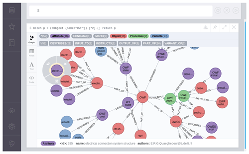
The screenshot of the server's web interface in Fig. 3 gives an example of what interacting with the graph database can look like.

2.2 Content in WESgraph

This section shifts focus to the content. This is not done by actually listing the contents, as that cannot be done in a manageable way; the actual database implementation is the most convenient approach to discover, browse, and otherwise query the database (access can be obtained by contacting the authors). Instead, Sect. 2.2.1 gives statistics, Sect. 2.2.2 lists the main sources for content, and Sect. 2.2.3 focuses on specific cases in which domain representation was not initially straightforward. For examples and illustration, we refer to the detailed description in Sect. 3.2.

Table 3 Database content node category numbers.

Figure 3 A screenshot of the Neo4j web interface.

2.2.1 Database statistics

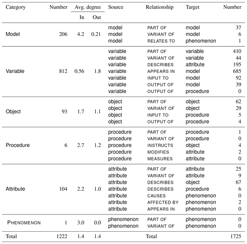
Currently, the database contains 1222 nodes and 1725 edges. Table 3 shows a breakdown over node categories. It is immediately apparent from the table that most database content is currently concentrated in the virtual world of models and variables.

2.2.2 Sources for content

Content can be added from various sources and in different ways:

• domain experts contributing directly to the database;

• database managers entering information obtained from domain experts;

• database managers copying knowledge from the literature; and

• database managers importing existing subdomain-specific databases or tool descriptions in a semiautomated way.

Adding content itself is straightforward, but its integration within the database requires creating extra nodes and connections and, to remove duplication, merging existing and new nodes. This is actually the conceptually hardest part when adding content.

2.2.3 Content representation challenges

As mentioned above, the integration of content can be conceptually challenging. This is because the different sources of content present the information in their own way, which is often not directly suitable for representation in a knowledge base such as WESgraph. This section therefore presents a number of practically relevant content representation challenges and proposed solutions.

Content harmonization

The content in the database is added by multiple people with different use cases for the database and originates from various sources. Even if the database schema and foundational ontology is adhered to, if no effort is made to integrate these additions, the database would become a disconnected bunch of graphs. This would defeat its purpose of being a coherent description of the wind farm domain.

Therefore, content must be harmonized to achieve this goal. Concretely, there are the following guidelines:

• a concept may only be represented by a single node, and

• tool-specific models and variables must be used sparingly and always described using part of or variant of relationships with generic models and variables.

Concept unicity and object multiplicity

The fact that each concept may only be represented by a single node has further implications. Namely, many objects in wind farms come in multiple instantiations, such as wind turbines and electrical cables. The fact that there are multiples of them plays a role in many models, such as those for calculating wake deficits and electrical losses. An approach must be used that acknowledges the inputs of those models and respects the unicity of concepts.

The chosen approach is to introduce

• “set of” variables to represent these – unique – sets of objects and

• “identifier” variables to refer to a specific instance of an object of which multiple instances are present in a wind farm.

Non-scalar variables

Scalar variables are trivial to represent, but this is not generally the case for non-scalar variables. Many models – certainly tools – deal with non-scalar variables of various types such as vectors, matrices, lists of instructions, and data sets. Some of these non-scalar variables also are closely related to models, and confusion may arise about how to include them in the database. Furthermore, when and how is a variable part of another variable?

The guidelines here are the following.

• Anything that is considered a variable of some form by a model for a part of the wind farm domain is a valid variable to be included in the database. This of course includes constants and parameters, but also files with input and output in some tool-specific format.

• A variable can be represented as a part of another variable if it is a distinguishable part thereof.

Variable connections of variant models

Multiple variants of a model can be added to the database. Even more so, it is actually a project goal to have such variants in the database to support analyses for which the performances of alternative models are compared. However, such variants will share many variables. The question then becomes how to connect those variables to all the variants.

The rule chosen is that variables must be connected to the most generic variant in which they appear.

Groups of models

The detail with which models and tools should be represented in the database has not yet been specified. In principle any level of detail can be used. It corresponds to the size of the set of interconnected models and variables that are used for it in the database. At one extreme, a single model with all the “externally” relevant variables corresponds to a high-level (rough) representation. At the other extreme, a large set of models and variables, most of which are “internal” in the sense that they are only connected to other models and variables within the set and not with externally relevant concepts, constitute a low-level (detailed) representation.

It can be useful to also have a high-level representation available for models that have been represented in high detail, for example to reduce complexity in analyses that do not require such detail. The approach implemented uses an extra overview model node of which the low-level models are made part of and which are labeled internal.

Disciplines

The wind farm domain is multidisciplinary. This means that the activities involved are diverse with respect to the background of the people performing them.

When using the database, it can be useful to focus on just one or a few of these disciplines. Therefore discipline labels have been added. They allow one to filter out nodes belonging to or not belonging to some disciplines.

2.3 Use cases

This section presents a non-exhaustive list of use cases.

Computation pathway discovery

In an analysis or design of a wind farm, a large number of models play a role. Furthermore, multiple sets of models can be used to achieve the same goals; call them computation pathways. The models in these pathways can vary in their fidelity and computational complexity. So the same analysis or design may be performed with varying computational time and result quality characteristics. Therefore, it is useful to be able to discover such pathways.

Consider the example given in Fig. 4. It shows three pathways for calculating the power output potential of a wind turbine (on the right) starting from the wind speed at its hub (on the left). The topmost pathway uses the turbine's power curve to directly calculate the output. The other pathways first pass via the power available in the wind at the rotor. Then the middle one directly computes the output from this using a power conversion factor. In the bottom pathway one more intermediate step is taken via the power extracted by the rotor, thereby separately considering the transformation from wind power to mechanical power and mechanical power to electrical power.

The subgraph of this example is the result of a multistep process. The generic version of this process is the computation pathway discovery activity. The process consists of performing online queries on the database and iteratively modifying these queries until the sought-for outputs, including subgraph visualizations and tabular listings, are obtained.

The calculation pathway discovery process is still a quite manual one and still requires some domain knowledge. But it is greatly facilitated by the graph database functionality. Namely, compare it to what would need to be done without the database: a combination of a literature study, interaction with experts, and ad hoc graph drawing to get a comparable result. Of course the quality of the result depends entirely on the amount of content in the database and the care with which it has been represented; this holds for this and all other use cases. However, the fact that the database can grow over time in a collaborative effort, is available to the entire community, and has multiple use cases makes the investment worthwhile.

Tool interoperability

There is a multitude of tools in use in the wind farm domain but no interoperability conventions yet. Some provide unique functionality and for some alternatives exist. They all work with the same general domain and therefore the many variables reappear as inputs or outputs. In principle they can be chained together in a workflow, or one tool can be replaced by another. However, this is hampered by the lack of interoperability conventions. Namely, a common ontology¹ of inputs and outputs and a common data exchange format are required.

WESgraph can facilitate efforts to create interoperability conventions. First of all, it can provide the common ontology; namely, its subgraph of variables is effectively such an on ontology, structured through its connection with the real world of objects, procedures, and their attributes. Tools are just model instances; using part of and variant of relationships they can be described to the level of detail required. The tool-specific inputs and outputs can be added as variables that are variants of the tool-neutral common ontology variables. These variant of relationships can carry – in their properties – the precise information necessary to transform common ontology variable values to tool-specific variable values.

Defining disciplines

As stated before, the wind farm domain is multidisciplinary. This use case concerns the problem of defining a useful set of disciplines. Previous work in this area has been done by Sempreviva et al. (2017).

What constitutes a useful set of disciplines? We use the following criteria.

1. Individual disciplines correspond to what is typically understood to be a discipline, namely a specific branch of knowledge, learning, and practice. In other words, each discipline represents a subdomain that can stand on its own as an object of study.

2. The set of disciplines covers the whole domain.

3. Each discipline covers a nontrivial part of the domain – that is, disciplines that cover almost all domain concepts or just a few domain concepts provide no added value and would crowd the set of disciplines.

4. The difference between any pair of disciplines is also nontrivial in the sense that a sufficient number of concepts should belong to one but not to the other. (This still allows subdisciplines.)

What comes to the fore in this set of criteria is a reliance on having an overview of the domain. This is what WESgraph provides. Discipline terms can be applied to concepts in the database (as labels), either to all or to a specific subset, such as all models. This way, a set of disciplines defined on WESgraph can be viewed as a high-level summary of information present in the database, namely of wind farm domain concepts. WESgraph can then be used to improve the set so as to better satisfy the criteria given above.

Education

In education, WESgraph can be used for domain discovery, that is, to learn about the different parts of the wind farm domain and how they are related. For example, it is possible to discover

• the different objects that together form the physical wind energy system,

• the different ways in which specific variables play a role, and

• the alternatives that exist for certain models.

One can imagine students doing a project in a certain subfield checking the database to see if they have not missed anything relevant, e.g., concrete variables, models, objects, and procedures, in their subfield or in related fields. This educational use case is not only applicable to students in the strict sense but to anyone needing to familiarize themselves with (a part of) the domain.

Figure 4 A simple WESgraph excerpt showing different pathways for computing the potential power output of a wind turbine (some edges omitted for clarity).

3 Detailed description

This second main part of the paper has the same general structure as the first, the general overview (Sect. 2). Namely, it dives deeper into WESgraph's structure (Sect. 3.1), content (Sect. 3.2), and use cases (Sect. 3.3).

3.1 The graph database structure of WESgraph

Each of the subsections of the general overview's discussion of the graph database structure has a counterpart here. Moreover, two additional subsections are present. Section 3.1.6 reflects on the schema and foundational ontology, and Sect. 3.1.7 discusses the usage of labels in the database.

3.1.1 Structuring content in a labeled property graph

This section provides further details and background for the material discussed in Sect. 2.1.1.

As mentioned there, the labeled property graph underlying WESgraph is a directed graph. Other, e.g., undirected, graph concepts exist, but this one supports the inherently directed nature of the relationships of WESgraph and knows various software implementations. In general, such directed graphs can contain multiple edges between the same pair of nodes and loops (edges between a node and itself). These may not be present in WESgraph. So ordered pairs of start and end nodes uniquely specify edges, which must be completed with a relationship type and, possibly, properties to become fully defined.

Section 2.1.1 listed two sets of rules to enable consistent use of WESgraph. In classical, often relational databases, the description of the database structure, including such rules (often called constraints), is its schema (see, e.g., Silberschatz et al., 2011). In the database world, this is widely understood as a formal machine-readable specification that is automatically enforced. Graph database software is often mostly schema-less in this formal sense. Nevertheless, a specification of the structure in natural language that users need to adhere to can act as an informal schema.

As said, WESgraph's database schema consists of two conceptually separable parts: the first is the foundational ontology (see, e.g., Staab and Studer, 2009). The design of (foundational) ontologies has become a proper research topic in some fields, such as cybersecurity (Iannacone et al., 2015). The second is an enumeration of properties. In practice, both parts cannot be completely separated, as the prescribed properties depend on the category and relationship type.

There has been previous work on creating an ontology for wind energy by Küçük and Arslan (2014), who generate theirs in a semiautomated way from text documents. However, it is a domain ontology wherein all the foundational ontology aspects are expressed using the differences between the relationships. There is no differentiation between the concept nodes as is done in this work using categories. Their domain ontology is more restricted in terms of content compared to the content in our database and in terms of scope, as it does not include models. Furthermore, Groza (2015) created a wind energy ontology with the specific aim of facilitating the development of small wind energy projects. Its aim differs from WESgraph, but its conception is interesting because it more directly allows for automated reasoning.

3.1.2 Categories

This section provides further background for the material discussed in Sect. 2.1.2.

Figure 5 Excerpts from WESgraph of the subgraphs defined by the part of relationship.

In the specification of the categories, expressivity must be balanced with simplicity. Expressivity pushes towards a larger number of categories. Simplicity favors a smaller set of categories that can be kept in mind by human users. The set of categories decided upon was determined by

1. the original use cases, which required a description of models for (offshore) wind energy subsystems and their interconnections through variables, and

2. the need to contextualize those models by relating them to the physical systems themselves.

This prompted the division into the virtual world and the real world visible in Fig. 2.

Even if the virtual world is the important part for the original use cases, but perhaps not for other potential uses of the database, the real world creates a mind map that supports users. This holds both for adding content to the database and querying the database. For example, having a “wind turbine rotor” object node as a starting point helps adding the variables and models that relate to it. Inversely, it also allows someone else to easily discover the variables and models in the database related to it.

3.1.3 Relationships

This section provides illustrations and some thoughts for the material discussed in Sect. 2.1.3. The relationships defined there are treated here in the same order.

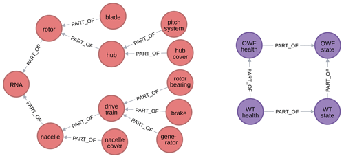
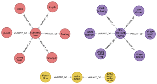
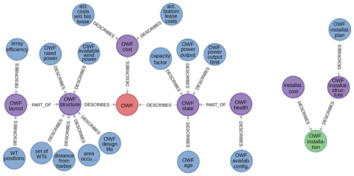
The part of and variant of relationships predominantly tend to create tree-shaped subgraphs. Namely, nodes are generally only part of or a variant of a single parent. However, this is not a strict requirement, and for some attributes it is even very sensible for them to be part of two parents. Figures 5 and 6 show excerpts of the subgraphs defined by the part of and variant of relationships. Figure 5 shows a tree-structured subgraph for object (on the left, red nodes) and an excerpt from the subgraph for attribute (on the right, purple nodes) in which a node with multiple parents appears. Figure 6 shows subgraphs for objects (top left, red nodes), attributes (top right, purple nodes), and models (bottom, yellow nodes).

Figure 6 Excerpts from WESgraph of the subgraph defined by the variant of relationship.

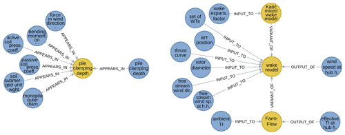
Recalling that the model category comprises both mathematical models and computational tools, it should come as no surprise that appears in is mostly used for the former and output of and input to are mostly used for the latter. Figure 7 shows excerpts of the subgraph of model–variable pairs. Specifically, on the left-hand side, it shows the use of the appears in relationship with a mathematical model (an implicit one for pile clamping depth). On the right-hand side, it shows the use of input to and output of relationships for computational tools (farm wake models in this case).

Figure 7 Excerpts from WESgraph of the subgraph of model–variable pairs.

Figure 8 Excerpts from WESgraph of the subgraph defined by the describes relationship.

Figure 8 shows excerpts of the subgraph defined by the describes relationship. On the left-hand side, it shows how the offshore wind farm object is described. On the right-hand side, it shows how the offshore wind farm installation procedure is described.

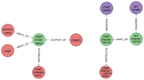
Figure 9 Excerpts from WESgraph of the subgraph defined by the instructs relationship and its context.

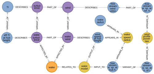
Figure 10 Subgraph defined a phenomenon, its affected by and relates to relationships, and its context (excerpt from WESgraph).

Figure 9 shows excerpts of the subgraph defined by the instructs relationship and its context. On the left-hand side, it shows a procedure whereby an object is created, namely the offshore wind energy system. On the right-hand side, it shows procedures whereby attributes are modified.

One could argue that it is not the procedure that modifies or measures, but the object that has been instructed. However, having procedure as the nexus for all relationships involved provides for more easily recognizable and less ambiguous connection patterns.

Finally, Fig. 10 shows an excerpt with the single phenomenon currently in the database – wake – with its affected by and relates to relationships as well as its context.

3.1.4 Properties

This section provides details omitted in Sect. 2.1.3.

Of the properties applicable to both nodes and relationships, authors is required for all of them so that the “ownership” of all database content is made explicit. Also, a description is in principle required for all nodes. Descriptions of models may include mathematical expressions, as long as the variable symbols used are also explained therein.

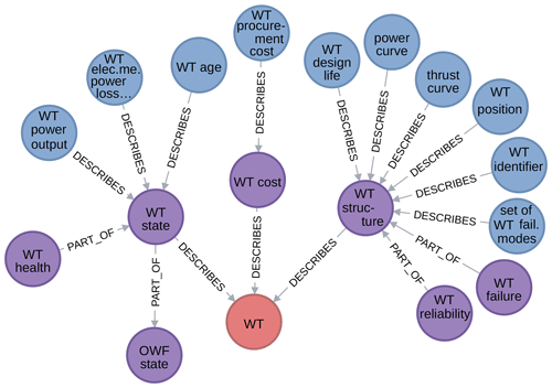
Regarding the name property: it must be unique for a given category to avoid ambiguity. If this name is judged sufficiently informative for some concept, its description may be omitted. In name, uniformly used abbreviations for words common in the database are encouraged to improve their usefulness when visualizing the graph: for example, WT for “wind turbine”. Furthermore, a convention for the name property of attributes that describe provides an additional schema rule: such an attribute is either a state, structural, or a cost. Their name must be the name of the concept they describe followed by one of those terms. This convention is used to force the many potential attributes into three subcategories, as this gives a better overview. An example of how this convention is implemented is given in Fig. 11.

The set of values for the name property form a so-called vocabulary for the wind farm domain (see, e.g., Gartner, 2016). Currently, these names are not assigned following existing naming conventions and given the value of brevity for graph visualization purposes, actually using such standardized names may not be practical. As a consequence, it is not guaranteed that a node can be found when searching for a standardized name. However, this can be remedied by adding a property that contains a dictionary mapping standards to names, following the example of Gancarski and Vasiljevic (2019).

Finally, a specific property has been defined for the appears in relationship between variables and models:

• output, holding a Boolean value (true or false) to indicate whether or not the connected variable is the usual output of the connected model.

Whereas the input to and output of relationships between variables and models unambiguously provide the role of the variables, appears in does not. The output property makes it possible to nevertheless encode the variable's typical role, which is essential to get a view of actual practice in the domain. It is therefore required to be present.

Figure 11 An example implementation of the top-level attribute state, structure, and cost name convention (excerpt from WESgraph).

3.1.5 Implementation

This section provides further details and discussion for the concrete implementation choice briefly introduced in Sect. 2.1.5.

The graph database Neo4j is cross-platform Java software available under both free and commercial licenses (Neo4j, Inc., 2019a). Interaction with the server can be done through a provided internet browser interface, application programming interfaces to various popular programming languages, or via HTTP requests containing JSON-formatted messages (ECMA International, 2017). Commands for the server are formulated in Cypher, a graph-database-specific query language (Neo4j, Inc., 2019b) comparable to what SQL (Structured Query Language) is for relational databases (Silberschatz et al., 2011). The content can be exported to various machine-readable and human-readable formats, such as JSON and GraphML (Brandes et al., 2002).

The main reasons for choosing this particular graph database software are

• its free license (AGPL version 3), taking away any cost considerations at this stage of development (FSF, Inc., 2007),

• its interactive web interface, which greatly facilitates interaction with the database, and

• its server nature so that multiple users can access the same database concurrently and from different locations.

Furthermore, it has good documentation, and the fact that it is one of the market leaders makes it straightforward to find support. Recall the screenshot of the web interface showing interactive functionality – graph element selection – in Fig. 3. It shows the command line box for entering Cypher queries (top), a menu bar for accessing database-related information (left), and a query result window containing an interactive graph visualization. All graph visualizations in this paper have been obtained as exports from this interface.

It does have some limitations, described as follows.

• The web interface provides no interactive editing of graph elements or properties. This must all be done using Cypher queries. However, there are separate tools that make this possible; these have not been tested.

• There is only very limited support for specifying a formal schema. Namely, only per-label property existence and uniqueness constraints can be added. Thus, most of the schema we specified must be respected through author discipline and periodic efforts by the maintainer to correct deviations from the schema.

3.1.6 Reflection on the schema and foundational ontology

The foundational ontology and other aspects of the schema were in large part designed in a few brainstorming sessions. Afterwards, informed by experience adding material to the database, they were further tweaked. Even if our experience shows that the current schema in general and the foundational ontology in particular provide a useful basis for a knowledge base, it is not set in stone and may evolve further. This paper describes the first public version: version 1.0.0.

While the schema design is informed by practical experience, that was not the driver. Examples of this are the elements in the foundational ontology that do not yet appear in the actual database, such as the measures relationship. In fact, the foundational ontology should drive the way content is added to the database. It should lead to the database being accessible to a relatively wide audience within the wind energy community. Therefore, it should be small and apprehensible without constant reference to an extensive specification; a diagram such as Fig. 2 should be sufficient for day-to-day use.

The downside of using a small, apprehensible foundational ontology is that it may be rather crude. For example, the subcategories of attribute do not really partition the set of all possible attributes. This can be illustrated using Fig. 11: “wind turbine reliability” is not completely structural, as implied by the current connections, but has state aspects as well. Furthermore, the foundational ontology does not provide guidance on many practical domain representation issues one encounters while adding content to the database. Such issues are discussed in Sect. 2.2.3 and 3.2.3. To underline the fact that our foundational ontology is indeed small, MarineTLO – a foundational ontology for the marine species domain – has 55 categories and 37 relationships (Tzitzikas et al., 2013), although it must be said that such numbers cannot be compared directly.

Even while keeping its content the same, the schema could have a different structure. Namely, in a graph database it is always possible to replace a node property by a node containing the property value and a relationship expressing the property type. For example, the unit property of variables could be replaced by a unit category and a has unit relationship. The same remark can be made about labels, for example, using discipline nodes (see Sect. 3.1.7) and relationships instead of labels. Such a design would add more structure to the database contents at the expense of increasing the number of categories, making the foundational ontology more complex.

3.1.7 Labels other than categories

Section 2.1.1 mentioned that an arbitrary number of labels can be added to nodes. The description of the foundational ontology in Sect. 2.1.2 already mentioned one application of labels: categories. Of these, one and only one must be added to each node. Labels are a convenient tool for other purposes as well. They appear in the database to indicate

• the discipline a concept belongs to (e.g., maintenance, electricity, mechanics),

• a related set of nodes whose addition to the database is being worked on, and

• the fact that a model or variable is internal to some larger, overarching model.

Apart from not creating “too many” labels, there is no guideline yet on what is and what is not a valid use case for non-category labels. Of the ones mentioned above, the labels indicating disciplines are meant to evolve into a standard set of disciplines that can be used as a categorization orthogonal to the one of the foundational ontology; there is more on this in Sect. 2.2.3 and 3.2.3. Whenever content is added to the database, labeling the nodes that are part of work in progress helps avoid edit conflicts and supports tracking them over multiple editing sessions. A reference to a common source (e.g., NREL cost breakdown) can, for example, be used for the label. When such work-in-progress content has been sufficiently integrated into the database, meaning that it does not duplicate existing nodes and is fully connected to the existing nodes, such a temporary label must be removed. Finally, the internal label provides functionality that supports properly representing large, modular models, but it is not yet clear whether it is a sufficiently effective approach; there is more on this in Sect. 2.2.3 and 3.2.3.

3.2 Content in WESgraph

The structure of this section perfectly mirrors the one found for its counterpart in the general overview (Sect. 2.2).

3.2.1 Database statistics

This section provides statistics beyond those mentioned in Sect. 2.2.1.

Table 4 shows a breakdown over node categories and edge relationship types. The average in-degree and out-degree for the different categories are also included. (The in-degree of a node is the number of incoming edges, and the out-degree of a node is the number of outgoing edges.)

Table 4 Breakdown of database content node and edge numbers.

We already remarked in Sect. 2.2.1 that most database content – 83 % of nodes – is currently concentrated in the virtual world. Table 4 also makes it clear that the part of and variant of relationships form a substantial part of all connections made for all categories except for procedures – 36 % over all categories. Furthermore, on average more than four variables are connected to each model; i.e., they have an average in-degree larger than four (the number of model–model relationships is negligible, relatively speaking).

3.2.2 Sources for content

Here we expand on Sect. 2.2.2 by describing our practical experience in adding content to WESgraph.

Initially, the authors added content reflecting their personal knowledge, supported by standard references such as the books by Manwell et al. (2009), Burton et al. (2001), and the collection edited by Twidell and Gaudiosi (2009). The first step was to develop the subgraph for object part of object, which describes the breakdown of the physical wind energy system. This created the context for adding and connecting some models. It included adding a few procedures to see how they could be integrated. Throughout this initial stage, the foundational ontology changed based on the experience and insight gained.

The initial stage gave way to trying out various approaches for obtaining and adding further content. One was gathering information about models used in the field by interviewing domain experts. Specifically, the wind energy group of ECN (Energy research Centre of the Netherlands, now part of TNO) contributed in this way. This led to general and also ECN-specific additions such as their FarmFlow wake modeling tool, shown in Fig. 12.

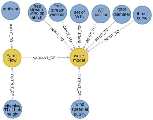
Figure 12 The model node for the FarmFlow wake tool and its surroundings in the graph (excerpt from WESgraph).

In the first of two trials for adding large bodies of content, the models described in the PhD thesis of Zaaijer (2013) were imported. This was done in a semiautomated fashion: to start, models from the thesis and the variables involved were manually copied to a structured spreadsheet description. This description was then imported to the database using a script, adding about 150 models, 330 variables, and 600 relationships. Finally, connections between imported nodes and those previously present were manually added to integrate the material. This integration is still an ongoing process and is not trivial; it effectively prompted the discussion on model grouping in Sect. 2.2.3 and 3.2.3.

The second large import was of the NREL cost breakdown for offshore wind farms (Moné et al., 2015, App. F). This time, the tabular structure could be readily copied to a spreadsheet and from there automatically imported using a script. Almost 350 cost variables were added in this trial, all part of a tree-shaped cost breakdown. This imported material has not yet been connected to the preexisting content.

The experience with the two import trials showed that it is straightforward to add content but that this is not the case for integrating the imported material. Integration usually requires adding new nodes that allow for the creation of relationships with the existing and imported material as well the merging of existing nodes to remove duplication. This is complicated by the lack of naming convention in the literature and often missing explicit definitions of variables such as cost components. Planning integration before importing can greatly reduce the effort required, as much of the needed work can be anticipated and taken into account in the spreadsheet structure and import script.

3.2.3 Content representation challenges

This section provides details, examples, and background for the representation challenges listed in Sect. 2.2.3. That section claimed that content integration in the database, and not its mere addition, is the major overarching challenge. Our experience supports this claim and shows that this is actually the most time-consuming activity when expanding the database content. One reason is that the content sources, such as a description of a set of models underlying a software tool (e.g., Zaaijer, 2013), provide a conceptually different view of the domain than the one presented in a knowledge base. For example, the choice of variables may be geared towards computation, and therefore, from the knowledge base perspective, issues such as the duplication of variables may be present.

Each of the choices made about how to deal with such issues needs to have general applicability throughout the database. These choices effectively correspond to a set of guidelines that, while not part of the schema or foundational ontology, should be followed in similar content representation situations elsewhere in the database. The reason is that they form consistency criteria that database users can rely on. Given their repeated application, it is useful to support the implementation of the guidelines with specific tools. This is, for example, possible using scripted workflows, providing a level of automation.

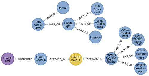
Figure 13 An example from WESgraph of concept duplication to be eliminated (CAPEX – capital expenditure).

For some of these cases, the issue at hand is still not resolved entirely satisfactorily.

Content harmonization

The guidelines given in Sect. 2.2.3 are

• a concept may only be represented by a single node, and

• tool-specific models and variables must be used sparingly and always described using part of or variant of relationships with generic models and variables.

Examples from the database can illustrate both of the above guidelines.

Figure 13 gives an example of concept duplication that should be eliminated. At the top of the figure is an excerpt from the NREL cost breakdown (Moné et al., 2015), with top-level cost nodes for the offshore wind farm, and at the bottom is an excerpt of the cost model of Zaaijer (2013), with top-level cost nodes for the offshore wind energy system; both are discussed in Sect. 3.2.2. The capital expenditure concept is duplicated, but not necessarily its part of children, so that some care needs to be taken in merging these two subgraphs – this still remains to be done. (Note that the part of relationship here has been used to indicate decomposition into terms of a sum. Such usage is ambiguous and should therefore, despite its convenience, be eliminated by adding intermediate sum models.)

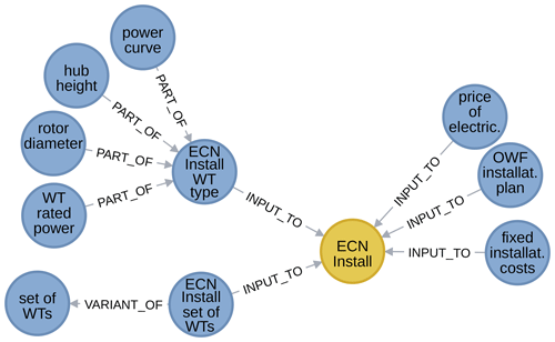
Figure 14 shows how tool-specific nodes can be handled. The example of the ECN Install tool is used. Here, the tool-specific input variables are described as either a variant of a generic variable or decomposed into generic variables using the part of relationship.

Finally, even while not being essential in their representation, the provenance of nodes should still be indicated in the description and references properties.

Concept unicity and object multiplicity

The approach presented in Sect. 2.2.3 is to introduce

• “set of” variables to represent – unique – sets of objects and

• “identifier” variables to refer to a specific instance of an object of which multiple instances are present in a wind farm.

Set variables can be found in many of the graph excerpts used as illustrations above: the set of wind turbines in Figs. 7 (right), 8 (left), 12, and 14; the set of transmission cable grid endpoints in Fig. 1; and the set of wind turbine failures in Fig. 11. That last figure also shows an identifier variable, the wind turbine identifier. However, no use of such a variable as input to or output of a model has yet been made, and they may still prove superfluous.

It is informative to take a closer look at the role set of transmission cable grid endpoints plays in Fig. 1. It is used to calculate the wind farm power output. Namely, it provides the information necessary to sum the right cable endpoint power flows. The reason for using cable endpoints and not cables in such a context is that the power flow in a cable is not constant due to losses, which we also need to be able to express.

Non-scalar variables

The guidelines given in Sect. 2.2.3 are the following.

• Anything that is considered a variable of some form by a model for a part of the wind farm domain is a valid variable to be included in the database.

• A variable can be represented as a part of another variable if it is a distinguishable part thereof.

A first comment here pertains to the fact that some tools can be extended with scripts included in input files; such things complicate the distinction between variables and models. A useful discriminator here is that anything that adds substantial functionality to a tool cannot be a variable but could perhaps be better dealt with using model groups (see below).

Next, how should variables that essentially contain all the information necessary to define some model be dealt with? Despite the apparent redundancy, the idea is to include both and, if needed, make their relationships explicit. This is best clarified and explained using an example. The graph on the left in Fig. 15 presents a few models and variables related to the power curve of a wind turbine. The power curve itself (in the middle) is represented as a variable – think about a list of wind speed and power output pairs. Two related models are shown: the one at the bottom transforms wind speed values into power outputs in conformance to the information specified in the power curve variable. The one at the top represents an algorithm that takes wind speed and power output pairs and produces a power curve variable. (Neither of these models is specified in a detailed way in terms of, for example, whether and how the conformity model interpolates; such detail is not needed in general but could be added if a database use case requires it.)

Finally, components of a vector and lines in a list or file are prime examples of variables part of variables. Figure 15 illustrates this with excerpts from the graph: from left to right, it shows how cut-in and cut-out speeds are features of the power curve, how a power curve is part of the ECN Install wind turbine description input, how an (ECN Install) offshore wind farm installation plan consists of distinct installation steps, how scale and shape parameters are features of a Weibull distribution, and how the free-stream wind velocity has speed and direction components.

Variable connections of variant models

The rule presented in Sect. 2.2.3 is that variables must be connected to the most generic variant in which they appear.

The reasoning behind this rule is as follows. Recall from Sect. 2.1.3 that a concept that is a variant of another concept should be more specific. If two variants cannot be ordered in this way, they should be represented as variants of a more generic common abstraction. Therefore, a set of variant nodes is (partially) ordered from most generic to most specific. In the context of models, this ordering can be exploited – using the rule – to limit the number of connections to shared variables and make part of the specificity of each variant immediately apparent. Then, to know all the variables involved in a specific variant, we can look at all the variables connected to that variant and any of its more generic “ancestors”. Also, those variables connected to this specific variant are then immediately known to be specific to it and all its “descendants” in the order.

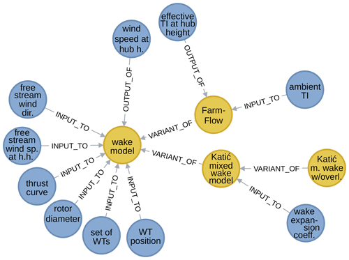
To illustrate, Fig. 16 shows an example of an ordered set of models and their variables. Namely, it shows a generic farm wake model (on the left), with its typical inputs and its output, and the disturbed wind speed at hub height. It has two more specific, concrete variants: the classical farm wake model by Katić et al. (1987) and FarmFlow (Brand and Wagenaar, 2010), ECN's farm wake model. Both have an extra input variable: a wake expansion factor and the ambient turbulence intensity, respectively. The latter also has an extra output: the effective turbulence intensity at hub height. Furthermore, the Katić model also has a variant with wind speed rotor plane averaging.

The variable connection rule must actually be made more precise. Above, it was assumed that the relationship type of the connection is the same between a model and its variant. In the case that it is not, the connection must not be omitted. For example, a variable that appears in a model may be an output of a variant of that model. So the variable connection rule must be applied to variables and relationship types, not just to variables by themselves.

Groups of models

Section 2.2.3 summarized the implemented approach for dealing with groups of models as follows: an extra overview model node is introduced, which the low-level models are made part of and which are labeled internal.

There are other potential approaches.

• Part of the complexity of model groups may be hidden using specifically tailored database queries. However, this cannot replace actually embedding domain knowledge.

• A natural way to implement the representation of models at different levels of detail would be to use a nested graph, namely, to embed a subgraph in a node – the overview model. However, support for nested graph functionality is not (commonly) available in graph database software, so an alternative was needed.

Considering the above, the approach implemented is the following.

1. Create the overview model node.

2. Add all models and variables of the low-level description, their interconnections, and connections to outside variables.

3. Connect all the low-level description models as part of the overview model and label them internal.

4. Label as internal all the low-level description variables that are output of some internal model. (The output of here should be understood to also include appears in with output set to true; the idea is to identify all variables that are produced internally.)

5. Also connect all non-internal variables connected to internal models to the overview model. Care must be taken to use the right relationship type, as it may change from the one used for the low-level connection it mimics, namely the following:

   • when output of is used in the low-level description, use output of;

   • when input to is used in the low-level description, use input to; and

   • when appears in is used in the low-level description, use

     • output of when the low-level relationship's output property is true and

     • input to when the low-level relationship's output property is false.

   The reason for this is that internal variables are unavailable when dealing with the overview model, and the input–output flexibility of an appears in relationship requires their availability. The overview model effectively behaves like a tool.

This approach makes it easy to filter out the internal nodes using the internal label and overview model. But at the same time, the low-level description is easily accessible. However, when adding connections from internal variables to external models, its internal label must be removed and appropriate connections to the overview model must be added.

The above approach was applied to the maintenance model of Zaaijer (2013, 239–243), which consists of 37 models, 36 variables, and 230 relationships. Of these variables, 34 are not internal. This model group is too big to show in its entirety, but Fig. 17 on the left gives an illustrative excerpt. In the middle is the overview model, with an internal model both to the left and to the right. On the extreme left and right are two internal variables, and above and below are four external ones. For these external variables, notice the difference in relationship type for connections with the internal model and with the overview model. Figure 17 on the right shows the same model but with internal nodes removed.

Disciplines

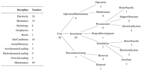
Section 2.2.3 mentioned that discipline labels can be added to enable the filtering out of nodes belonging to or not belonging to some disciplines. In practice, such labels were applied to the models imported from the thesis of Zaaijer (2013), as discussed in Sect. 3.2.2, and correspond to the titles of the sections used there to list these models. These discipline names are listed in Table 5, where the numbers of models that have been labeled as belonging to the discipline are also listed; the disciplines that are effectively cost categories are presented hierarchically, mirroring how they have been used.

For this strategy to be effective, disciplines must be assigned to all nodes or perhaps all models, which is currently not the case, and they should correspond to subsets of the domain that are meaningful to the users of the database. Furthermore, they should provide added value and not duplicate information already readily available. The set of disciplines used in this case was chosen in an ad hoc fashion and can be improved upon.

Actually, creating a proper set of disciplines is a task of its own, whereby not only a set of discipline names must be decided on, but also relationships between disciplines and the assignment of disciplines to nodes. Our limited experience indicates that qua structure a partially ordered set of disciplines works well. For example, as can be gathered from the cost category decomposition on the left in Table 5, some nodes are effectively labeled with the “Procurement” subcategory (of “Investment”) and also with “SupportStructure”. WESgraph can actually support this task of creating a set of useful disciplines; Sect. 3.3.3 discusses how.

Figure 14 An example of limiting tool-specific variable nodes (excerpt from WESgraph).

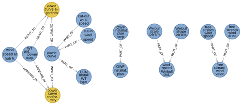
Figure 15 Examples of non-scalar variables and their surroundings in the graph (excerpt from WESgraph).

Figure 16 Example of an ordered set of variant models and their variables (excerpt from WESgraph).

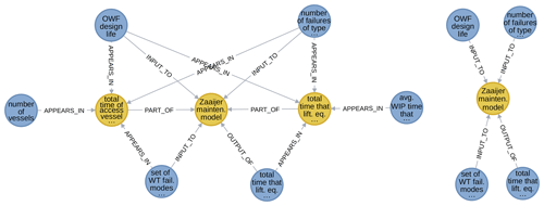
Figure 17 WESgraph excerpt showing an overview model and part of its low-level description (a). The same, except with internal nodes removed (b).

Table 5 Discipline and cost category labels used. (The prefix “Cost” has been removed from lower-level cost categories for brevity.)

3.3 Use cases

This part goes into the details of the use cases that Sect. 2.3 lists; each one now gets its own section. Section 3.3.1 discusses the discovery of computation pathways, the use case that actually triggered WESgraph's development. During WESgraph's development three other use cases became apparent to us: Sect. 3.3.2 discusses tool interoperability, Sect. 3.3.3 discusses the definition of a coherent set of disciplines for the wind energy domain, and Sect. 3.3.4 discusses education.

3.3.1 Computation pathway discovery

This section makes the steps present in the computation pathway discovery use case discussed in Sect. 2.3 and illustrated by Fig. 4 explicit. It also discusses the relevance of this activity for multidisciplinary design analysis and optimization (MDAO).

We mentioned that computation pathway discovery is a multistep process. This process is facilitated by the interactive functionality of the database software's web interface, that is, the possibility of exploring the neighborhood of query result nodes in a point-and-click fashion. Next to exporting the result of this process, one can also save key queries in the process for later reuse, for example after new content has been added to the database.

The qualitatively distinct steps in the computation pathway discovery process are the following.

1. Decide which variables are the focus of the investigation. These are typically inputs (what one has available for computing with) and outputs (what one wishes to compute) but can also involve intermediate variables. In the example, this would be “wind speed” and “power output”.

2. Perform a keyword-based query for each of these variables of interest to see which concrete variables there are in the database. The query may need to be refined to get a more relevant set of matches. Based on the results, concrete variables are selected that will function as endpoints – or junctions – in the pathways. In the example, the initial keywords could be “wind speed” and “power”, with, for example, the latter refined to “WT power”. The selected variables are “wind speed at hub height” and “WT potential power output”.

3. Perform a query to search for a shortest path between endpoints traversing any junction nodes. In the example, the shortest path will be the top one, passing through the power curve conformity model; it has a length of two.

4. Query for paths of increasing length, starting from the shortest path length. To keep the output manageable, queries looking for paths such as this one may often need to be refined to exclude or only include certain node categories or nodes from being present in the result. An upper limit on the length is decided on a case-by-case basis, typically informed by the results already observed. For the example, the node categories were restricted to variables and models, which is typical if the focus is really on computation. Furthermore, some nodes were excluded, such as the “set of WTs” variable, that created paths that did not correspond to actual computational pathways. So in this part of the process, the middle length-four and bottom length-six pathways were discovered.

5. Finally, discover which other nodes are relevant using the interactive interface. This exploration of the neighborhood of pathways can be as extensive or concise as desired. In the example, only variables needed to complete the set of inputs of the individual models in the pathways such as “power coefficient” were added in this way.

Not all calculation pathway analyses fit into the mold sketched above. For these, the process will remain generally similar but should be adapted. An example is the situation in which one considers only an output variable and is interested in sets of inputs that allow it to be computed. In this case, instead of starting from a shortest path between nodes and increasing the path length, one can start by considering incoming paths of length one and increase their length, again excluding unwanted paths by refining the query.

The discovery of computational pathways is particularly useful for informing the possibilities for system scope and model fidelity while building MDAO workflows.

Multidisciplinary design analysis and optimization (MDAO) is a systems engineering technique that exploits the interactions between technical disciplines and the design of different subcomponents to solve trade-offs in the benefit of the performance of the entire system. MDAO workflow is the term given to the coupling of computational models driven by algorithms that solve a use case: optimization, for example. The complexity of MDAO workflows can be categorized along three axes: system scope, model fidelity, and MDAO architecture. System scope encompasses the choice of disciplines and subcomponents that are modeled in the MDAO workflow, model fidelity stands for the level of sophistication of the models coupled in the MDAO workflow, and MDAO architecture is the logical flow of data between modules and between the algorithms and the modules.

Depending on the use case to solve, for example the minimization of the levelized cost of energy (LCOE) of a wind farm with respect to the position of the wind turbines (layout), one would typically be interested first in finding which disciplines or subcomponents are affected by the wind farm layout and which of these impact the LCOE. Of the entire list of variables, a wind farm designer can then short-list those necessary to evaluate the performance of a particular subcomponent and select a subset of the variables deemed most impactful. Then, finding the paths between those variables and the LCOE variable informs which models (disciplines or subcomponents) can make the link.

Concerning model fidelity, if there are two or more paths (two or more sets of models) that link certain input and output variables, WESgraph can provide the required inputs and the available outputs of each of these models. If users have a list of variables at their disposal, a query of WESgraph can provide information on what data are missing and which variables will not be needed.

Additionally, WESgraph could be queried by MDAO workflow-manipulating software to automate the creation of workflows given a use case (see van Gent et al., 2017). Hence, if one can formalize the description of a use case using such software by including the objective function, constraints, and design variables, WESgraph can provide the knowledge of which models can be coupled and which would require more input data from the user.

3.3.2 Tool interoperability

This section provides background and some further thoughts about the tool interoperability use case discussed in Sect. 2.3.

The advent of more integrated system-level design and analysis has brought to the fore the advantages of interoperability conventions. Concretely, the current IEA Wind Task 37, Wind Energy Systems Engineering: Integrated RD&D, which the authors are involved in, has as one of its objectives to “provide framework guidelines that will enable more seamless integration of analysis tools and reference models between organizations” (see also  Sanchez Perez-Moreno et al., 2016). Specifically, in its Work Package 1, the goal is to develop the necessary common ontology and common data exchange format. This is comparable to the goal of the Common Parametric Aircraft Configuration Schema (CPACS, 2019) for aircraft design. The experience of the people working on this ontology and the data exchange formats is that it is a daunting task to be sufficiently comprehensive.

As said, WESgraph can facilitate efforts to create interoperability conventions by specifying tools (models) and their variables as variants of tool-neutral counterparts. This makes it possible to automate the creation of common data exchange format descriptions, for example using the JSON Schema language (Wright et al., 2019). It even opens up the possibility of automating data format translation.

The development of common ontology variables closely relates to the issue of the integration of new tools in WESgraph, discussed in Sect. 2.2.3 and 3.2.3. The duplication of concepts as well as name conflicts are solved by a naming convention for tool-neutral variables.

3.3.3 Defining disciplines

This section provides concrete pointers on how to use WESgraph to create and improve a set of disciplines for the third use case discussed in Sect. 2.3. It also discusses the added value of using WESgraph for this purpose. Earlier, Sects. 2.2.3 and 3.1.7 mentioned that labels can be used to indicate the disciplines a node belongs to and that these can be used to filter the database content. Section 3.2.3 made this more concrete by showing what disciplines are currently present in WESgraph.

To bootstrap the discipline definition activity, an initial proposal set of disciplines is formulated by domain experts, for example, by taking the taxonomy of Sempreviva et al. (2017). These are then applied as labels to the concepts in the database. This makes it possible for the following criteria to be checked and improvements to be applied:

• in the case that some concepts are not covered by any discipline term, a discipline needs to be added or broadened in scope;

• in the case that a discipline covers almost all or just a few concepts, it can be removed, or, in the latter case, it can be decided that concepts need to be added to the database to improve its coverage of the domain;

• in the case that a pair of disciplines both cover essentially the same concepts, they either need to be merged or concepts need to be added to the database to differentiate the disciplines;

• in the case that the majority of concepts in a discipline are connected to concepts in another discipline, it should be investigated whether the disciplines should be merged;

• in a discipline, if there are hardly any connections between one set of concepts and another, it may need to be split.

The second and third point make it clear that adding disciplines to WESgraph can cause underrepresented domain areas to become apparent. For the last two points, clustering algorithms for graphs may be used. The database queries for checking the above criteria could even be integrated into a semiautomated workflow that proposes changes to a set of disciplines, functioning as decision support for domain experts.

When one arrives at a set of disciplines built from the above steps, each discipline effectively corresponds to a nontrivial and unique set of concepts. It may reflect biases present in the database because, for example, some part of the domain is underdescribed, but these can be reduced to the degree desired by expanding the database. Biases and other defects in a set of disciplines defined solely on the basis of expert opinion are hard to concretely discuss, as justification for this set is typically limited (e.g., mostly inside the expert's head or informal). When using WESgraph the disciplines are backed by sets of concepts, providing a very concrete justification by definition through enumeration. This improves the chances of the set of disciplines being accepted and used by the community.

3.3.4 Education

This section makes the last use case discussed in Sect. 2.3, education, more concrete and notes how it can also facilitate the improvement of the database quality.

When learning using WESgraph, users will in practice start with a simple query to obtain a single or a few nodes. Then they can use an interface (see Fig. 3) to explore the connections of the nodes obtained. This exploration can be repeated to explore an arbitrarily large part of the database. The interface makes it possible to remove nodes from view so the graph excerpt shown can be kept to a manageable size. For each of the nodes, their properties, especially the description and references, provide information that goes beyond what can be learned from the connections and name alone.

There is already enough content for pilots of this use case, but for actual use the content still needs to grow and mature.

There is an advantage to this use case: during their explorations, the students will encounter issues, such as errors and omissions. If appropriate procedures and facilities are put in place, such as a bug tracker, they can signal and help fix them. So this use case can actually help improve the quality of the database content.

4 Conclusion and vision

This paper started by stating that a tool that enables researchers in the wind energy field to keep the overview can provide great benefits. This paper describes WESgraph, a knowledge base for the wind farm domain, which is a tool made just for that purpose. Its conception as a graph database allows us to make use of functionality in existing software that facilitates access to the content (Sect. 3.1.5 and 3.1.5). The design of its structure balances the requirements of expressivity and simplicity to enable a broad group of practitioners to both make use and contribute (Sects. 2.1 and 3.1). Although the database content itself was not a focus of this paper, it does discuss and provide solutions for non-straightforward domain representation cases (Sects. 2.2.3 and 3.2.3) to provide an accurate view of the difficulties that arise when adding content to the database. The paper describes a number of different use cases to make clear not only what WESgraph is, but also how it can be used.

So, this work shows that it is possible to build a tool that helps people keep the overview of the wind farm domain. The actual benefits of this tool are greatly dependent on the amount and quality of the database content. Our experience in adding data, as reported mainly in Sects. 2.2 and 3.2, makes it clear that adding content is a time-consuming but mostly one-time activity. Our current judgment is that the time investment – also for management – will only really pay off if a larger group of people contribute and make use of the database. Each contributor can focus on their areas of expertise, making content addition more time-efficient. Each successful use case increases the value of the database and therefore decreases its relative time investment cost.

Therefore, we see the future of WESgraph as a shared resource built by an international online community led by a core group exercising quality control. Such a community can increase the accessibility of the database by creating effective documentation, providing instruction, and facilitating collaboration between people with a specific use case and people with experience in using the database. Such collaborations are important because there is an appreciable learning curve, which will never completely disappear, even if more beginner-friendly software tools for accessing the database become available. Successful community building and the maintenance of a shared knowledge base can effectively avoid the duplication of structured domain description efforts of various research and working groups that would otherwise create single-use spreadsheets.