the Creative Commons Attribution 4.0 License.
the Creative Commons Attribution 4.0 License.
 | 05 Mar 2020
Optimizing wind farm control through wake steering using surrogate models based on high-fidelity simulations
Paul Hulsman
Tuhfe Göçmen
This paper aims to develop fast and reliable surrogate models for yaw-based wind farm control. The surrogates, based on polynomial chaos expansion (PCE), are built using high-fidelity flow simulations coupled with aeroelastic simulations of the turbine performance and loads. Developing a model for wind farm control is a challenging control problem due to the time-varying dynamics of the wake. The wind farm control strategy is optimized for both the power output and the loading of the turbines. The optimization performed using two Vestas V27 turbines in a row for a specific atmospheric condition suggests that a power gain of almost 3%±1% can be achieved at close spacing by yawing the upstream turbine more than 15∘. At larger spacing the optimization shows that yawing is not beneficial as the optimization reverts to normal operation. Furthermore, it was also identified that a reduction in the equivalent loads was obtained at the cost of power production. The total power gains are discussed in relation to the associated model errors and the uncertainty of the surrogate models used in the optimization, as well as the implications for wind farm control.
- Article
(4530 KB) - Full-text XML
- BibTeX
- EndNote


Wind turbines operating in the wake of upstream turbine(s) experience power losses and increased fatigue loads. Accordingly, wind farm control aims at improving the power production and potentially decreasing structural loads by optimizing the collective operation of the wind farm, as well as providing better integration of wind power into the grid. Intentionally yawing the turbine has been the focus of recent studies as one of the methods to mitigate the wake effects. The objective is to intentionally change the trajectory of the wake in order to increase the power output of the downstream turbine(s) and possibly reduce the fatigue loads.
However, in order to apply yaw-based wind farm control, a thorough understanding of the wake and the loading on the wind turbine components is necessary. The earliest studies investigating the performance of a propeller in yaw were conducted by Ribner (1943), Anderson (1979), and Smulders et al. (1981). Recently the concept of yawing the turbine has gained renewed interest focusing on the effect of the wake on downstream turbines. The characteristics of the wake have been analysed in various studies, e.g. Knudsen et al. (2015) for an overall review. Numerous wind tunnel experiments have shown the potential of redirecting the wake, e.g. Medici and Dahlberg (2003), Medici and Alfredsson (2006), and Bartl et al. (2018a). Fleming et al. (2014) evaluated different techniques to redirect the wake using high-fidelity simulations and concluded that yaw misalignment has the most promising potential. Gebraad et al. (2017) showed that this can potentially increase the power output and the annual energy production (AEP) of the total wind farm.
However, these numerical studies are computationally demanding, while dynamic wind farm control requires fast and reliable wake models in the optimization loop. Therefore, engineering models which capture the effects of wake steering are necessary. Jiménez et al. (2010) developed such a model to describe the wake deflection. This was combined with a multi-zone wake deficit model in FLORIS (FLOw Redirection and Induction in Steady State). The FLORIS framework, see Annoni et al. (2018), now includes an alternative wake model by Bastankhah and Porté-Agel (2014), which is further extended in Bastankhah and Porté-Agel (2016). However, FLORIS yields time averaged results for power prediction, while a model that combines the estimation of both power output and the structural loading on the wind turbine is crucial in order to apply yaw-based wind farm control. The majority of the studies have only implemented the power gain in the cost function; see Gebraad et al. (2016), Fleming et al. (2016), Kragh and Hansen (2015), and Gebraad et al. (2017). However, van Dijk et al. (2016) combined the FLORIS framework with the CCBlade model in order to analyse the impact of yaw control on the power output as well as turbine loading. Their results show that a decrease in loading is possible at the cost of a reduction in the power production.
This study aims to develop and validate yaw-based wind farm control strategies, based on surrogate models through the use of the high-fidelity flow solver EllipSys3D LES (large eddy simulation) and the aeroelastic tool Flex5. A surrogate model essentially constructs response surfaces based on the input and output of the determined domain. Both the power output and the turbine loading are included in the optimization and assessment of different wind farm control settings. The analysis also highlights the advantage of using the surrogate models as compared to the conventional analytical models in the optimization.
2.1 High-fidelity simulation of wind turbine wakes and wind turbine response
The turbulent wake behind a wind turbine is simulated using EllipSys3D and the actuator line method to represent the turbine, while the turbine performance and response are calculated using the aeroelastic tool Flex5. These tools and methods are briefly described in the following; for a more comprehensive description, see Sørensen et al. (2015).
2.1.1 Large eddy simulation
Large eddy simulations (LESs) have been performed with EllipSys3D, which was developed at the Technical University of Denmark by Michelsen (1992) and by Sørensen (1995). EllipSys3D solves the discretized incompressible Navier–Stokes equations in general curvilinear coordinates using a block-structured finite volume approach. The large-scale turbulence is simulated directly by the Navier–Stokes equations, whereas the turbulence eddies smaller than a predefined grid size, Δx, are modelled using a subgrid-scale model. The incompressible and filtered Navier–Stokes equation is given in Eq. (1), and the continuity equation is given in Eq. (2). Here, is the filtered velocity vector, x is the position vector, is the filtered pressure, ρ is the density, ν is the kinematic viscosity, t is the time, and f represents external body forces. The external body forces are used to represent the turbine and the atmospheric boundary layer and to impose turbulence, and these body forces will be described in more detail in Sect. 2.1.2, 2.1.3 and 2.1.4. A hybrid scheme formed from a third-order QUICK scheme (Leonard, 1979) and fourth-order central differencing scheme is used to discretize the non-linear terms.
2.1.2 Prescribed boundary layer
The atmospheric boundary layer is modelled by using body forces (fPBL) throughout the computational domain. This makes it possible to model the shear profile and the atmospheric turbulence independently as described in Troldborg et al. (2014) and to apply any arbitrary wind shear (and potentially veer) profiles; see for instance Hasager et al. (2017).
2.1.3 Atmospheric turbulence
Turbulence is introduced to the Navier–Stokes equation by imposing body forces (fturb) into the flow applied in a plane upstream of the turbine; see Gilling et al. (2009). The imposed turbulence fluctuations are obtained from a Mann turbulence box; see Mann (1994) and Mann (1998). The model requires three input parameters: , LTurb, and γ, where αTurb is the Kolmogorov constant, ϵ is the rate of viscous dissipation of specific turbulent kinetic energy, LTurb is the turbulence length scale, and γ is a measure of turbulence anisotropy.
2.1.4 Rotor modelling
The wind turbine is modelled using the actuator line method (AL), as developed by Sørensen and Shen (2002) and implemented in EllipSys3D by Mikkelsen (2003) and Troldborg (2009), which imposes body forces (fWT) along rotating lines in the numerical domain. Here, the actuator lines are coupled to the aeroelastic tool Flex5 developed by Øye (1996), which gives the aerodynamic forces on the rotor blades and deflections; see Sect. 2.1.6.
2.1.5 EllipSys3D setup
The numerical domain used for the simulations is in the streamwise, lateral, and vertical directions, respectively. The grid points are equidistantly distributed in a central region of the domain, where the turbine and wake are located. The central region is located at and the mesh is stretched outside of the central region towards the boundaries. The domain consists of grid points for a total of approximately 34×106 grid points. The grid resolution in the central region corresponds to 22 cells per blade, which implies that the simulations do not capture distinct tip vortices from the individual blades. However, the curled wake and the otherwise detailed wake dynamics are captured, which is used as input to the subsequent aeroelastic simulations. The simulated inflow is converted to a polar coordinate system in order to perform the simulation in Flex5. A convergence study was performed to determine the required number of radial and azimuthal stations in the polar coordinates, which showed that 10 radial stations and 36 azimuthal stations were sufficient.
Cyclic boundary conditions have been applied on the lateral boundaries, no-slip on the bottom, and far-field conditions on the top boundary. The prescribed atmospheric boundary layer profile is shown in Fig. 1, including the standard deviation and the rotor area. Furthermore, no veer has been imposed in the current simulations.
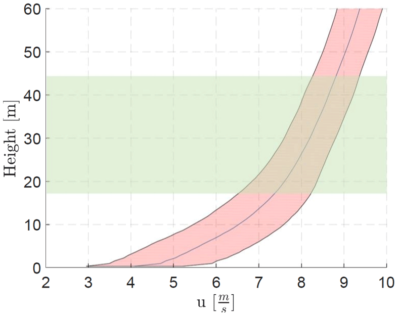
Figure 1Prescribed boundary layer in EllipSys3D. The shaded red area indicates the wind profile ±σ. The green area represents the rotor area.
The Mann box has been generated using the following parameters: m4∕3 s−2, LTurb = 156.69 m, and τ = 3.0516. All simulation cases are performed with the same turbulence seed, i.e. the exact same inflow, which enables direct comparison between the different yaw settings. The initial transient as the wake develops throughout the domain has been discarded, so each simulation is run for a total time of 1362 s (≈22 min).
2.1.6 Flex5
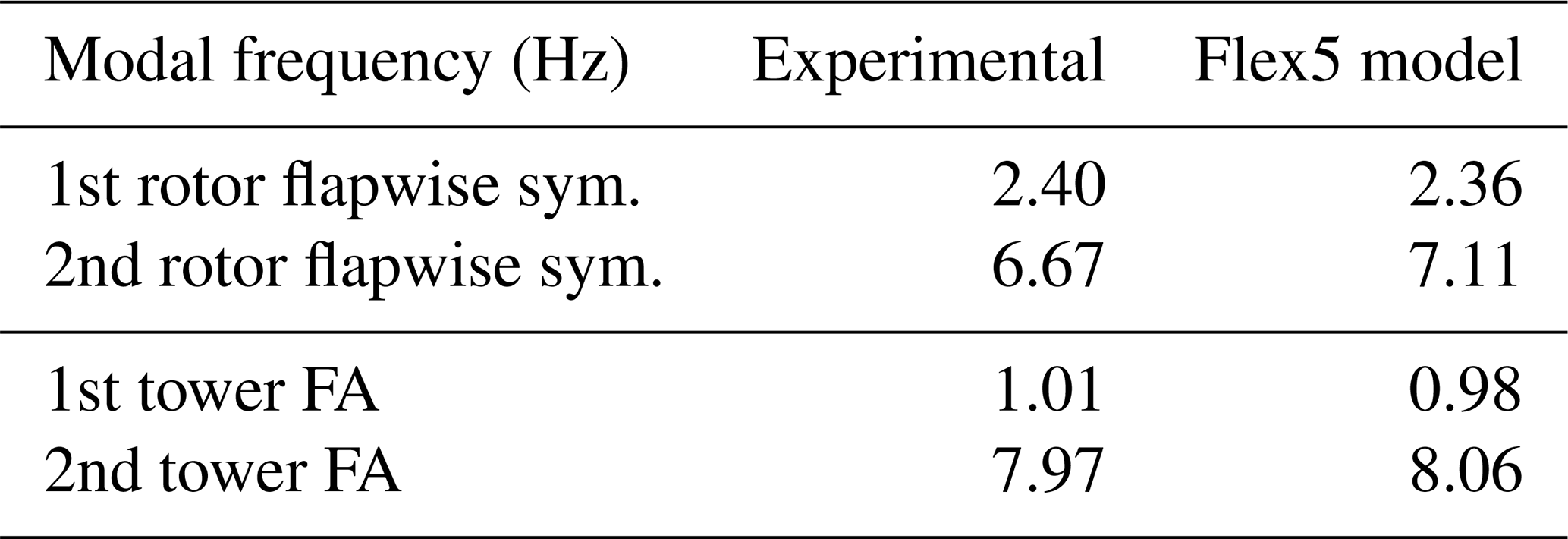
For the simulations in EllipSys3D, a Flex5 model of the V27, which is based on the V27 turbines located at the SWiFT facility as described by Resor and LeBlanc (2014), is used. The main parameters of the V27 wind turbine are given in Table 1, indicating the rated wind speed (Urated), the rated power (Prated), the rated rotor speed (wrated), the rotor radius (R), the hub height (HHub), the tilt angle (θTilt), and the tip speed ratio (λ). The eigenfrequencies are calibrated according to the reported experimental values and show a good match as given in Table 2.
Table 1Main parameters of the Vestas V27 given in Resor and LeBlanc (2014).
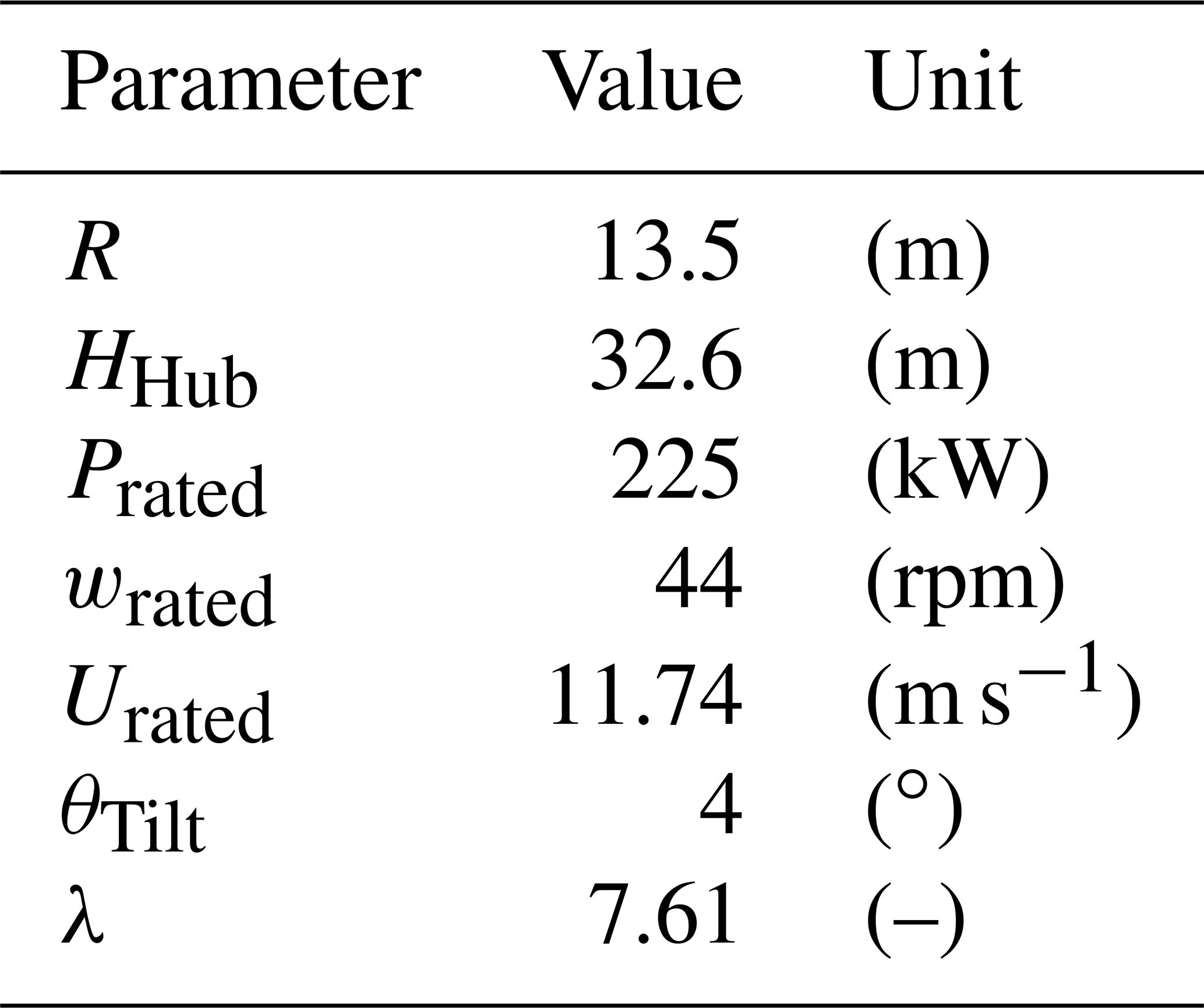
Table 2Calibration of the V27 model based on the experimental data from Resor and LeBlanc (2014). “FA” indicates the fore–aft motion of the turbine.
2.2 FLORIS setup and turbine recalibration
FLORIS1 is an engineering model aimed at estimating the wake deficit and the trajectory behind a yawing turbine. FLORIS contains various wake deficit models, see Annoni et al. (2018), yet only the Gaussian wake model is used here for further analysis.
The input parameters for FLORIS are determined from the EllipSys3D setup. Furthermore, the turbine characteristics, shown in Table 1, together with the CP and CT curves of the V27 are also used as input. The parameters PP and PT, which characterizes the power loss due to yaw misalignment and tilt angle, are recalibrated for the V27 using Flex5 under uniform and steady inflow. The parameters PP and PT are determined for the V27 turbine as 1.4 and 1.25, respectively, with η=1. These are lower compared to the values of the NREL 5 MW, which has a value for PP and PT equal to 1.88. Note that the calibration is limited to PT and PP for this study, and the default parameters reported in Annoni et al. (2018) are used for wake deflection and velocity deficit estimations.
2.3 Surrogate model
The main purpose of a surrogate model is to build a model that defines the relationship between the input and the output of a given data set in a fast and accurate manner. In the recent study of Dimitrov et al. (2018), six surrogate models were benchmarked in terms of their ability to predict the lifetime fatigue loads. The benchmark recommended using the polynomial chaos expansion (PCE) as the most beneficial surrogate method for quick assessment of loads. PCE is a powerful surrogating technique which aims to provide a functional approximation of a computationally complex model through its spectral representation on a basis of polynomial functions. Considering a set of independent stochastic variables, X, described by the joint probability density function, f(X), and a computational model as a map, Y=ℳ(X), the PCE of ℳ(X) can be defined as
where Φα(X) are multivariate polynomials which are orthonormal with respect to f(X), α ∈ 𝒩 is a multi-index that indicates the components of the multivariate polynomial Φα, and yα represents the corresponding coefficients which are iteratively determined. Due to its simplicity and fast convergence, the PCE is also widely used in comparison to a full Monte Carlo simulation; see Murcia et al. (2018) and Sudret (2008). In this study, it is used to create a response surface of the DEL and the power output obtained from Flex5 with inflow generated by LES.
The surrogate model was built using the python software toolbox Chaospy (http://chaospy.readthedocs.io/en/master/installation.html#from-source, last access: 7 May 2019), which is a numerical tool that enables uncertainty quantification using PCE and the advanced Monte Carlo method. It was first introduced by Feinberg and Langtangen (2015). Furthermore, the point collocation method is used to build the response surface of the surrogate model. It is a non-intrusive method which builds upon the idea of fitting the polynomials to the input variable by solving a linear system arising from a statistical regression. The response of the surrogate model is build via orthogonal polynomial families using the three term recursion relation, which depends on the selected distribution of the input parameters. For statistically independent distribution of the input parameter, a multivariate polynomial expansion in Chaospy can be created using the tensor product rule of univariate polynomials described in Feinberg and Langtangen (2015). The standard statistical linear regression approach is used to fit the polynomial sets, Φα, to the given set of data points, which determines the final coefficients of the surrogate model, yα. The order of the polynomial sets needs to be defined, which influences the output of the surrogate model.
2.3.1 Surrogate training data set
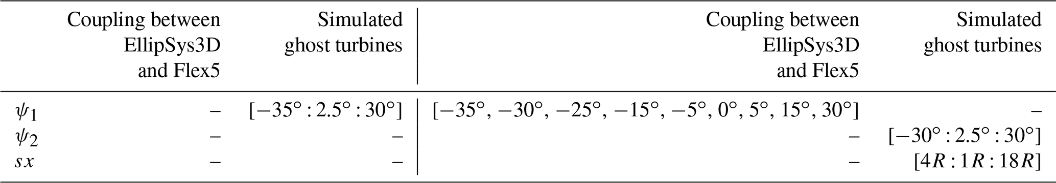
The training data for the surrogate models for the upstream and the downstream turbine are obtained from simulations performed with the aeroelastic tool Flex5. These simulations have been run using detailed turbulent inflow generated via EllipSys3D with a single turbine operating at different yaw misalignment. The angle between the rotor axis and the free-stream velocity is denoted by ψ. A positive yaw angle is a clockwise rotation of the turbine and a negative yaw angle is a counterclockwise rotation viewed from above. A total of nine simulations are performed with yaw angles of the upstream turbine of , −30, −25, −15, −5, 0, 5, 15, 30∘. Turbulent flow fields are extracted and used as input to Flex5 for different downstream turbine distances, . Hence, the downstream turbine does not affect the flow, and it is therefore denoted as a “ghost turbine”. A ghost turbine is indicated in Fig. 4, where the planes of the velocity components are extracted. The downstream ghost turbine is modelled for yaw angles of , −27.5, …, 30∘. An additional simulation was performed in EllipSys3D with no turbine, where the flow in the turbine position was extracted and used as input to Flex5 to create the surrogate for the upstream turbine. This was done to ensure a similar model error and uncertainty between the surrogate of the upstream and downstream turbine, which is particularly critical for the comparison and normalization of the results.
Table 3 gives an overview of the simulated cases. This created 27 combinations for the upstream turbine and combinations of yaw angles and downstream distances for the downstream turbine, which are used as input to train the surrogate models.
Table 3Overview of the cases simulated with the coupling between EllipSys3D LES and Flex5 and the cases simulated with the extracted flow field in Flex5.
2.3.2 Surrogate model setup
Surrogate models have been created for the power and the damage equivalent loads (DEL) for both the upstream and the downstream ghost turbine pair. Together with the produced power, only the DEL of the flapwise root bending moment and the total bottom tower bending moment are used to assess the effect of the yaw angle. This was done in order to simplify the model and to include the most important DEL influenced by yaw steering. The models are constructed using three input parameters: the upstream yaw angle (ψ1), the downstream yaw angle (ψ2), and the spacing between the upstream and downstream turbine (sx). Each input parameter is assigned a distribution, for the upstream and downstream yaw angle (ψ1 and ψ2) a normal distribution with μ=0∘ and σ=4.95∘ is used. These values are derived from the distribution of the wind direction at hub height in the LES. A uniform distribution is used for the turbine spacing, since the downstream distance is fixed at a certain location.
Three unique surrogate models for the upstream turbine were created for the power as well as the DEL for the flapwise root and the tower bending moments. Note that these upstream surrogate models only depend on the upstream yaw angle (ψ1). Another three surrogate models are created for the downstream turbine. However, the output of these models depend on the upstream yaw angle (ψ1), the downstream yaw angle (ψ2), and the spacing between the turbines (sx). The surrogate models are created with the numerical data between . Figure 2 gives an overview of the various surrogate models created, the output and the corresponding distribution of the input parameter from which the multivariate polynomial sets are built.
In addition, the stability of the surrogate models are improved by increasing the number of data points. Multiple realizations are extracted from the time series of Flex5 using a moving average with a window of 10 min shifted every 30 s. Therefore, there are 23 individual points for each unique configuration. This results in and = 149 040 data points for training. The input variables were normalized (or scaled) for the creation of the surrogate model in order to give each parameter equal weight, hence avoiding the potential bias in the model towards one parameter. As a result, the output is also normalized, but its scale is inverted to give the absolute values during the analysis of the results.
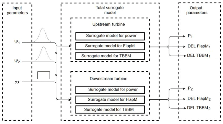
Figure 2Overview of the created surrogate models for the upstream turbine and the downstream turbine. The distribution of the upstream yaw angle (ψ1) and the downstream yaw angle (ψ2) is set to be Gaussian, and the spacing between the upstream and the downstream turbine (sx) is set to have a uniform distribution. The surrogate models account for the power, the DEL of the flapwise root bending moment (FlapM), and the DEL of the tower bottom bending moment (TBBM) of the upstream and the downstream turbines.
The example data set and the script for the surrogate model training can be found at the project git (https://github.com/Paul1994H/PCE-surrogates-for-power-and-loads-under-wind-farm-control.git, last access: 13 November 2019).
First, the turbine performance, wake deflection and velocity deficit is analysed for different yaw angles and downstream distances. Then the surrogate models for the upstream and downstream turbines are created, analysed, and used to optimize the operation of the turbine pair, which is examined in terms of uncertainty and model errors.
3.1 Turbine performance
The power output of the upstream turbine for the yaw cases ∘ and ψ1=0∘ is shown in Fig. 3. The power production is initially smooth before the imposed turbulence reaches the turbine and the wake starts to develop. The power output is clearly dynamic, and it is evident that the power production of the yawed turbine is significantly lower than normal operation. Interestingly, a reduction in the power fluctuations can also be observed for ∘ operation case but further investigation of that phenomenon is left as future work. The transient period of 100 s is indicated by the dotted line, and it has been discarded from the analysis, resulting in a total simulation time of 1261.62 s (≈21 min).
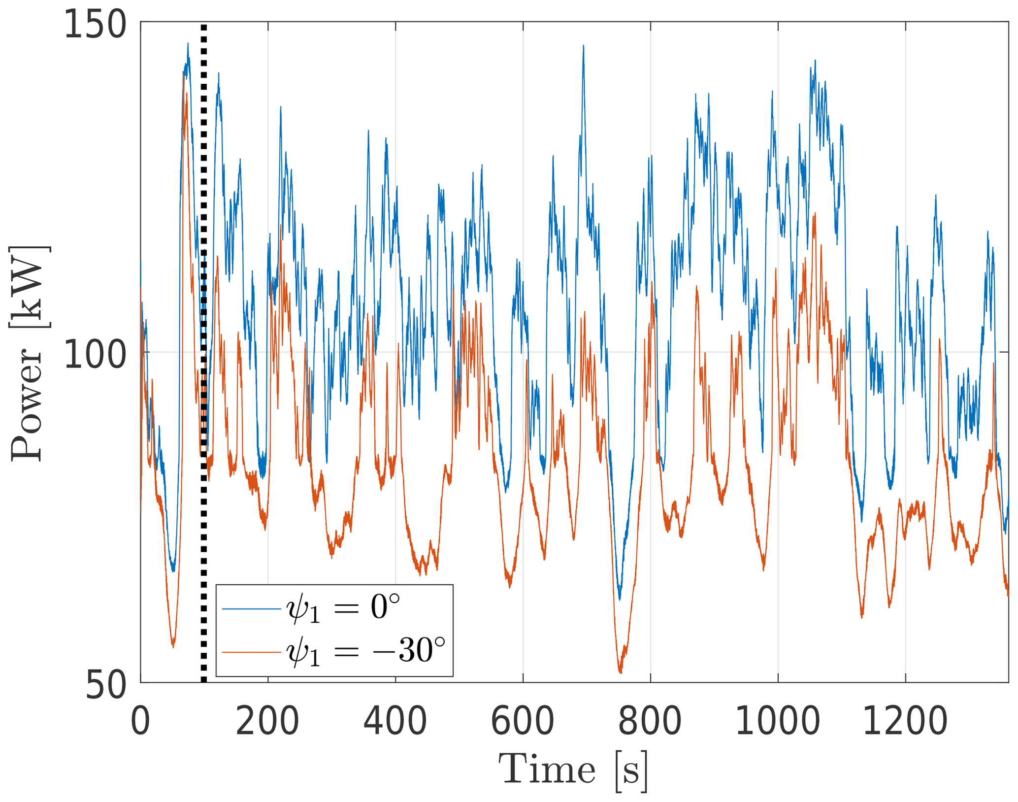
Figure 3Time series of the power output of the upstream turbine determined with the aeroelastic tool Flex5 at ψ1=0∘ and at ∘. Dotted lines indicate the end of the transient period
3.2 Wake deflection and velocity deficit
As the turbine is yawed, the inflow is no longer aligned with the rotor axis. The misalignment leads to a difference in the axial induction and thus an asymmetric loading on the rotor blades; see Branlard (2017). Additionally, the total thrust also decreases, as demonstrated in Bastankhah and Porté-Agel (2016). Bastankhah and Porté-Agel (2016) also illustrated how the wake deflection increases with increasing yaw angle. The wake is deflected as a yawed turbine exerts a lateral force on the incoming flow, which induces a spanwise wake velocity due to the conservation of momentum.
The deflected wake extracted from EllipSys3D is shown in Fig. 4 for ∘, ψ1=0∘, and ψ1=30∘. The figures show the average relative velocity () at hub height behind a single turbine. Here, u∞ is the average incoming streamwise component at hub height. The asymmetric wake is clearly visible; see Fleming et al. (2018) for more details. It is also evident how negative yaw angle leads to a higher deflection compared to a positive yaw angle.
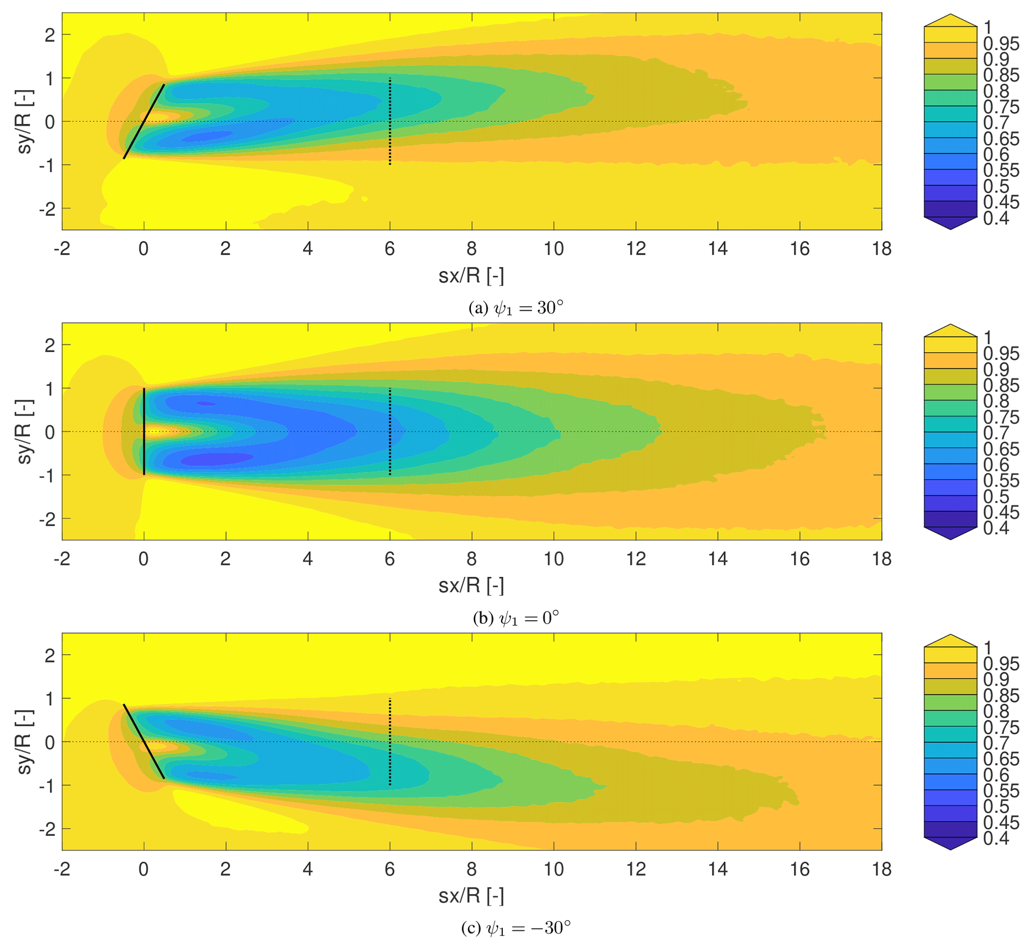
Figure 4Time averaged horizontal plane of the averaged relative velocity () at hub height extracted from EllipSys3D, where the upstream turbine is yawed (a) ψ1=30∘, (b) ψ1=0∘, and (c) ∘.
3.3 Power surface
3.3.1 High-fidelity simulation results
Figure 5 shows the cumulative power production of the two turbines for three different upstream yaw angles (ψ1) as a function of turbine spacing and downstream turbine yaw angle ψ2. The cumulative power production has been normalized by the power production of the upstream turbine with no yaw misalignment (i.e. ψ1=0).
The cumulative power output increases for increasing turbine spacing as expected since the wake recovers. Bastankhah and Porté-Agel (2016) showed that an increase in the yaw angle leads to a decrease in the power output, which is also seen in Fig. 5. The reduction in the cumulative power output is even more pronounced at large yaw angles of the downstream turbine, ψ2, as the power decrease for a yawed turbine operating in wake is increased compared to a freestanding turbine; see Liew et al. (2019). Furthermore, the effect of wake deflection is clearly visible in Fig. 5. The cumulative power output at ∘ and ψ1=30∘ is higher compared to ψ1=0∘ at ∘, −27.5∘, …, 30∘ and . The increased power production is due to the wake deflection observed in Fig. 4, where a higher velocity reaches the rotor of the downstream turbine. At ∘ the wake is deflected further away, which results in a higher power output for the downstream wind turbine at closer spacing in comparison to ψ1=30∘. In addition, the highest power output of the downstream wind turbine is obtained at a slight positive yaw angle for the downstream turbine (ψ2). This is indicated with the red line in Fig. 5, showing the yaw angle with the maximum power at a certain turbine spacing. The highest power production is achieved when the wake is approaching the rotor plane perpendicular. For ψ1<0∘, this results in ψ2>0∘; for ψ1>0∘, this results in ψ2<0∘. The minor increase in total power production by yawing the downstream turbine as well might not require additional control. In fact, it might rather be the preferred control setting of the downstream turbine even with a greedy controller, as the turbine aims to align itself with the flow automatically. Turbines reorienting themselves to improve power performance while operating in wake have also been observed in full-scale measurements by McKay et al. (2013) and experimentally observed by Bartl et al. (2018b).
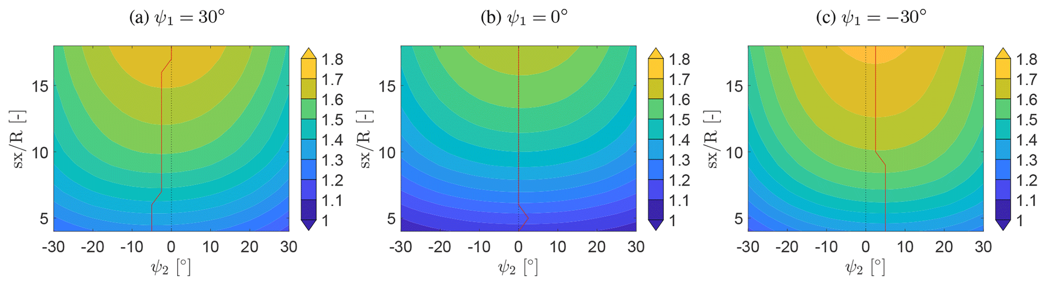
Figure 5Normalized cumulative power of the upstream and downstream turbine determined with the numerical simulation performed in EllipSys3D coupled with Flex5 at ∘, 0∘, 30∘ with different spacing and yaw angles for the downstream turbine. The cumulative power is normalized with the power output of the upstream turbine with no yaw misalignment (ψ1=0∘). is the downstream distance. ψ1 is the yaw angle of the upstream turbine. ψ2 is the yaw angle of the downstream turbine. The red line indicates the yaw angle with the highest power output at each downstream position.
3.3.2 FLORIS results
An increase in the cumulative power production for larger turbine spacing is also seen in the FLORIS results (not shown for brevity). However, as the FLORIS model does not capture the asymmetric behaviour of the wake deflection, the cumulative power at ∘ is identical to ψ1=30∘. Furthermore, the effect of a higher power output with a small yaw angle for the downstream turbine is not captured by the FLORIS model, as FLORIS uses the local free stream velocity described in Gebraad and Van Wingerden (2014). Furthermore, the assessment showed that FLORIS is unable to capture the velocity distribution within the near-wake region, but it otherwise shows a similar behaviour as the high-fidelity numerical simulation in the far-wake region.
3.3.3 Surrogate results
The results of EllipSys3D presented in Sect. 3.3.1 are used to build surrogate models for the upstream and downstream turbine using PCE as described in Sect. 2.3 and 2.3.1. The surrogate models are then used in optimization to find potentially beneficial wind farm control strategies. The analyses of the wake deflection and normalized velocity (Sect. 3.2), as well as the power output (Sect. 3.3.1), will aid the evaluation of the outcome of the optimization performed with the surrogate model, with regards to the power and the fatigue loads.
Here, the generated surrogate models are response surfaces based on multivariate polynomials. These response surfaces are highly dependent on the selected polynomial order and the available training data. To visualize the dependency of the generated PCE surrogates to the polynomial order and input data, an example case is used. The example case is based on the power of the downstream turbine at sx=5R where the upstream turbine yaw angle is fixed. Two sets of surrogate models are built with two different data sets in order to assess the sensitivity of the surrogates to the amount of training data and the polynomial order. The first surrogates exclude the data points at ∘ and ∘ shown in Table 3, while the second set of surrogates is built using the full data set. Both sets of surrogate models are constructed with polynomial orders of .
The response of the surrogate model is illustrated in Fig. 6. The black points show the power output obtained from different 10 min periods, which have been extracted using a moving average with a window of 10 min shifted every 30 s over the time series to increase the stability of the model. Therefore, there are 23 individual points, which are not statistically independent, but give an indication of the inherent variability. The red points indicate the median values of the simulation point at every unique condition. Figure 6a shows the first power surrogate built on the reduced data set. The surrogate models with p=5 and p=6 show signs of over-fitting between ψ1 = [−30∘, −15∘] and between ψ1 = [15∘, 30∘] for p=5. This tendency is general throughout the domain, although shown here only for a particular spacing (sx=5R) behind the upstream turbine.
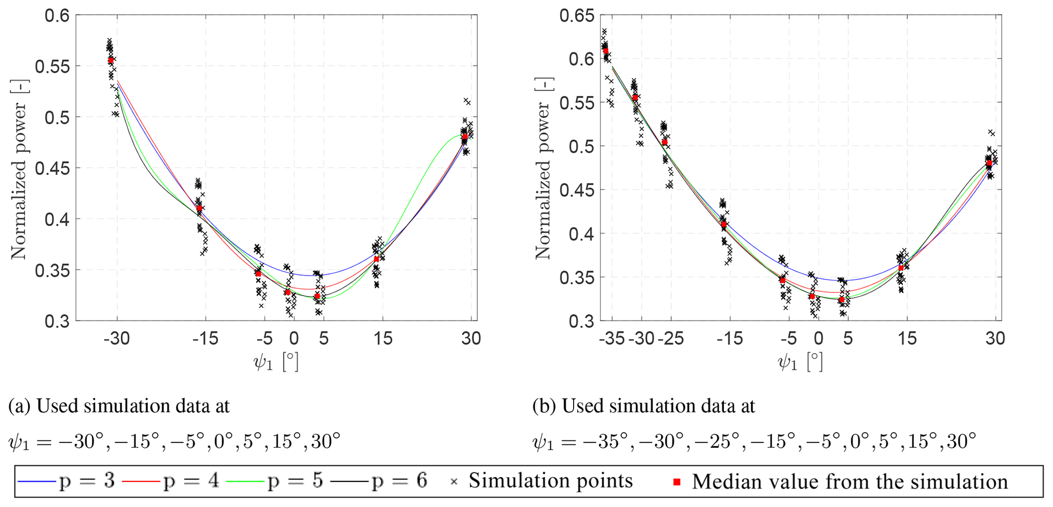
Figure 6Power output of the surrogate model of the downstream turbine at sx=5R and ψ2=0∘ with two different data sets. The surrogate model has been build using the PCE approach with different polynomial orders (p). Black: the crosses indicate the data points obtained by performing a moving average of 10 min shifted every 30 s. Red: the squares indicate the mean of the data points obtained by performing a moving average.
The over-fitting, which results in large errors in the estimates, can be reduced by populating the training data set further. Figure 6b shows the second set of power surrogates for the full training data set. It highlights how including more data increases the reliability of the fitted polynomial surfaces for all orders of the surrogate models (). However, at an order of p=6 the surrogate model still shows a sign of over-fitting in the following interval: ψ1 = [15∘, 30∘]. The output of the surrogate model of the order p=6 differs by approximately 7.5 % with the addition of ∘ and ∘ realizations to the training data set at . For the surrogate model of the order p=5, a difference of 6.4 % was observed. Over-fitting is therefore a significant risk when fitting higher-order polynomials to insufficient data or fairly simple response surfaces and when employing surrogates for extrapolation. On the other hand, it is also seen in Fig. 6b that the lower-order polynomials are unable to fully capture the deepest normalized power surface where ∘.
This also indicates that in order to develop a surrogate model based on simulation data, a trade-off needs to be made between an acceptable error, the polynomial order, and the cost of high-fidelity simulations. The surrogate models built with the entire data set (as illustrated in Fig. 6b) are used for the optimization of wind farm control strategies.
3.4 Relative error
The polynomial order for the PCE approach also has to be determined. Therefore, the relative error of each surrogate model with different polynomial orders is examined. The relative error is computed for each turbine spacing (ξR) and given by Eq. (4).
The relative error is the difference between the output of the surrogate model (PSM), with various polynomial orders, and the median of the 10 min power output from the simulations performed with Flex5, , where the flow field is extracted and used as an input to the aeroelastic tool. The error ξR is calculated for the entire domain of the optimization variables, including all the available combinations of ψ1 and ψ2 per downstream distance sx. Therefore, it reflects the overall sensitivity of the model performance to the control set points. The relative error in the power output of the downstream turbine is shown in Fig. 7. Here it can be seen that the distribution of the relative error for all ψ1−ψ2 combinations is wider at close spacing for each surrogate model, i.e. as the second turbine is within the near-wake region (up to ≈6R) of the upstream turbine. At larger spacing, the distribution gets narrower, indicating an increased confidence in the model performance for all ψ1−ψ2 combinations for larger turbine spacing.
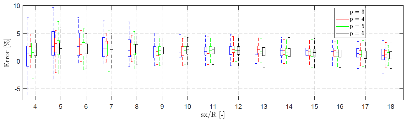
Figure 7Box plots of the relative error, ξR, of the power output of the downstream turbine between the surrogate model with orders of and the results obtained from the simulations performed with Flex5, where the flow field is extracted and used as an input to the aeroelastic tool. The distributions correspond to all the available combinations (225 in total) of the optimization variables ψ1 and ψ2 for each turbine spacing sx.
As discussed previously, there is a trade-off between acceptable error and polynomial order, but no decisive conclusion can be drawn with regards to the ideal polynomial order to build the surrogate models. The error distribution of all polynomial surrogates are comparable, and the median relative errors are generally decreased continuously from 3 % at sx=5R to approximately 1 % further downstream. Therefore, the surrogate models of polynomial order p=3 and p=4 are used in the optimization process due to the robustness of the lower orders against over-fitting (as discussed in Sect. 3.3.3) and for simplicity. Additionally, it should be noted that the consistent behaviour of ξR further downstream indicates a relatively low sensitivity of the surrogate model performance to both the optimization variables ψ1 and ψ2 and to the turbine spacing. This is highly beneficial for a robust optimization process.
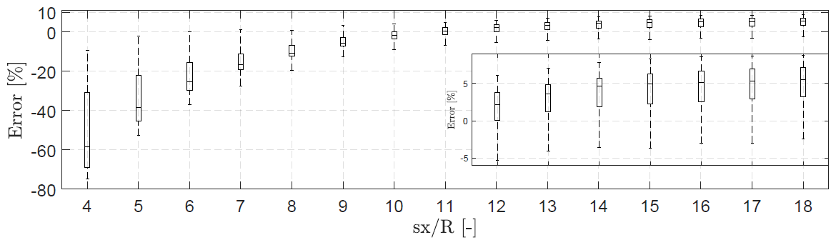
Figure 8Box plots of the relative error of the power output of the downstream turbine between the FLORIS model and the results from the simulations performed with Flex5, where the flow field is extracted and used as an input to the aeroelastic tool. The distributions corresponds to all the available combinations of the optimization variables ψ1 and ψ2 for each turbine spacing sx. The insert shows the zoom of the last box plots.
For comparison, the relative error between the simulations performed with Flex5 and the results obtained from the FLORIS model is shown in Fig. 8. The relative error is significant within the near-wake region, but it reduces to approximately 5 % further downstream for all the available combinations of ψ1−ψ2. Recent developments of the FLORIS model framework could potentially decrease the relative error, e.g. Martínez-Tossas et al. (2019). However, new additions to FLORIS still rely on model calibration against LES-generated data, which could equally be used to increase the population data for building surrogates as previously shown.
3.5 Optimization based on the surrogates
The optimization of wind farm control strategies is performed by applying a weight factor assigned for each surrogate model depending on the objective of the optimization. The aim of this study is to showcase how to develop a control strategy, which considers both the loads and the power output through the use of surrogate models. The weighting used for the optimization is shown in Eq. (5), where SM indicates the surrogate model.
Note that the weights of the surrogate models for the equivalent loads are subtracted from 1 since the aim is to reduce the fatigue loads. The optimal point is determined by calculating the power and the equivalent loads for the upstream and downstream turbines using the trained surrogates with input parameters of ψ1 = [−35∘ : 0.12∘ : 30∘], ψ2 = [−30∘ : 0.12∘ : 30∘], and . The optimal control set point is determined using the standard built-in max function in python. The optimal control strategy is determined for three cases:
-
a power-driven optimization
-
a combined load and power optimization with a large weight attributed to the power
-
a combined load and power optimization with a small weight attributed to the power
3.5.1 Power-driven optimization
The power-driven optimization is performed using Eq. (5) and setting n1=1 and with the order of p=3 and p=4 surrogate models for the upstream and downstream turbines. The results of the power-driven optimization are presented in Fig. 9. It shows the contribution of the upstream and downstream turbine to the total power gain, which is the ratio of the estimated power output from the surrogate model to the baseline (with ψ1=0∘ and ψ2=0∘) power production from the surrogate model; i.e. .
Figure 9 also depicts the optimal yaw angles of the upstream (ψ1=Opt) and the downstream (ψ2=Opt) turbines that maximize the cumulative power output. Both surrogate models predict that optimal power gain is obtained when the upstream turbine is yawed negatively and the downstream turbine is yawed slightly positively. This is in line with the power output shown in Sect. 3.3.1, where the highest power is obtained when the downstream yaw angle (ψ2) is slightly positive. This occurs as the second turbine aims to reorient itself to be perpendicular with the skewed inflow (see Fig. A1 in the Appendix A, which shows the average flow angle).
It is observed that the power gain is the largest at a turbine spacing of sx=4R with a power gain of approximately 1.6 % and 3.3 % for the surrogates of order p=3 and p=4, respectively. The difference in estimated power gain is directly related to the overestimation of power production for the baseline of the second turbine in Fig. 6 for p=3, which results in the reference PBase being too large. Otherwise, the optimization with both surrogate models of order p=3 and p=4 yield very similar predictions as the turbine spacing increases. Further downstream, the differences in both power gain and yaw angles of the two turbines are minor.
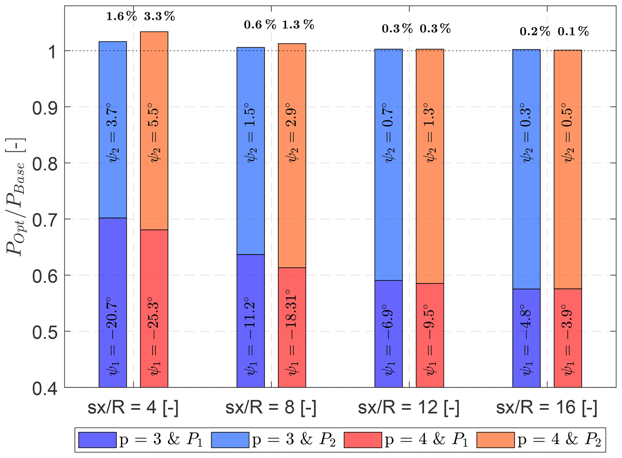
Figure 9Optimal yaw configuration and power gain for a power-driven optimization. Each bar indicates the cumulative power gain (POpt) normalized with the power of the respective turbine at a certain turbine spacing with no yaw misalignment (PBase), estimated by the surrogate models for both of the turbines. Darkened area: normalized power of the upstream turbine. Shaded: normalized power of the downstream turbine.
A negative yaw angle for the upstream turbine is expected as it yields a larger wake deflection (as shown in Sect. 3.2). Furthermore, the optimal yaw angles decrease in magnitude for both of the turbines as the turbine spacing is increased. This occurs as the power loss of the upstream turbine is larger than the power gain of the downstream turbine, which leads to a decrease in the optimal yaw angle of both turbines. However, the uncertainty increases as the yaw angle of the upstream turbine decreases, because intentionally yawing the turbine only approximately −4∘ in the case of sx=16R is uncertain as the inflow wind direction will continuously change, e.g. Gaumond et al. (2014), and the unintentional yaw misalignment due to erroneous wind direction measurements are often in a similar range, e.g. Mittelmeier and Kühn (2018).
As shown in Fig. 7, the surrogate models come with relative errors as a function of the control variables ψ1 and ψ2, which generally indicates an over-prediction of the power production. After the optimization is performed in Fig. 9, a closer look to the surrogate model error, ΔPOpt, for each of the optimal control settings is required to correct the model results for potential bias. ΔPOpt is defined in Eq. (6) in terms of ψ1=Opt and ψ2=Opt.
where
Since the dynamic Flex5 simulation gives different results for each 10 min realization (as can be seen in, for example, Fig. 6b), the model error also varies among those realizations. Note that the Flex5 results are not available for all combinations of ψ1 and ψ2, which is why the surrogate models are built in the first place. However, the prediction error of the surrogates for each turbine spacing can be interpolated for the optimized yaw angles ψ1=Opt and ψ2=Opt to estimate ΔPOpt. Median and standard deviation of the model error with respect to the reference Flex5 simulations are presented in Fig. 10a as a function of turbine spacing.

Figure 10Surrogate model error and estimated power gain likelihood for the optimized yaw settings ψ1 and ψ2 as a function of turbine spacing for PCE model orders p=3 and p=4. Error bars indicate the median ±1σ of the difference of the 10 min median realizations compared to the surrogate estimates.
Figure 10a shows that the surrogate models generally reproduce the optimum power very well. For PCE order p=3, the median error increases further downstream, where the optimization settings get closer to the baseline (i.e. ψ1=0∘ and ψ2=0∘). This behaviour is expected as it was also observed in Fig. 6b for ψ1=0∘ ± 15∘ and ψ2=0∘. There, it is also seen that the over-prediction is much less visible for PCE order p=4 in that region, which results in much smaller bias for the surrogate especially for larger turbine spacing. The error bars indicate 1 standard deviation of the surrogate model error compared to the median of the 23 different 10 min realizations. It shows that the surrogate model error easily both over- and under-predicts by 2 %, for a specific 10 min realization. Since the variance in the surrogate model error is purely due to the physical dynamics of the inflow used in the Flex5 simulations, and not the complexity of the surrogate, the spread around the median error for PCE orders p=3 and p=4 is essentially the same.
The surrogate model error is subsequently used to assess the power gain likelihood, ℒ(ΔP), which is the power estimate including the observed modelling error and uncertainty, as defined in Eq. (6). The expected power gain likelihood is obtained by subtracting the interpolated surrogate model error (shown in Fig. 10a) from the power gain predicted by the surrogate models for each turbine spacing and optimal yaw settings . In other words, due to the potential bias in the model results and difference over the 10 min realizations, implementing the optimum settings indicated in Fig. 9 gives a different power output, which is a source of uncertainty around the expected power gain by the surrogates. To take this bias and variability into account, the likelihood of the power gain is quantified based on the difference between the surrogate model performance and 10 min realizations of Flex5 simulations as in Eq. (6) and shown in Fig. 10b. It is highly important to note that the quantification of the “power variability” here in this study is limited to the difference between 10 min realizations. Inter 10 min statistics (or faster timescale investigations) and the ultimate dynamic evaluation of wake steering wind farm control is left as future work.
First and foremost, Fig. 10b shows a very similar power gain likelihood for both PCE surrogates p=3 and p=4, also in the near wake; though the results without taking the model error into account were very different as shown in Fig. 9. This shows the importance of the model correction in estimating the true power gain to be achieved by the optimized control settings estimated by the surrogate models. Note that in this study true power gain refers to the power gain that is observed in Flex5 simulations, as an approximation to real power gain that one would expect to be able to measure in the field, provided there were sufficient time, money, knowledge of techniques, etc., and no errors in the reporting, collection, and processing of the data. For both of the models p=3 and p=4, the power gain likelihood is higher (slightly less than 3 % ± 1 %) around the near-wake region, where it quickly drops to less than 0.5 % around 10R downstream. It is also seen that the standard deviation of the power gain is higher for p=4, which is due to the higher model complexity, hence higher sensitivity to the model inputs and higher optimum yaw angles up to 12R downstream as presented in Fig. 9. Both the expected power gain in Fig. 9 (before the model correction) and the power gain likelihood in Fig. 10b (after the model correction) point to essentially zero power gain after 10R for the investigated setup. It is mainly due to the fact that the optimized yaw setting ψ1 and ψ2 approaches the baseline case ψ1=0 and ψ2=0 for larger turbine spacings, i.e. no yaw on either turbine. For closer spacings, the wake dynamics are more complex and the associated uncertainty is significant. The analysis shows that the decision-making process to implement the control settings should be based on the power gain likelihood, where the model results are corrected with the best available information rather than an operational judgement based purely on the model results.
The uncertainty is partly due to the natural variability of the flow and the turbulent wake and partly due to the uncertainty associated with the surrogate models. The former is inherent and difficult to reduce, while the latter can be reduced by adding more high-fidelity data as shown in Sect. 3.3.3 and increasing model accuracy. The inherent uncertainties due to the natural variability of the non-stationary atmosphere compared to the current LES model setup are not fully accounted for and atmospheric stability is not included, either. Furthermore, the data used for the surrogates does not take the induction into account, i.e. the presence of the turbines alters the inflow and hence the actual power production, e.g. Troldborg and Meyer Forsting (2017) for steady state alterations and Mann et al. (2018) for changes in the incoming turbulent structures.
It should also be noted that wider error distributions and higher bias (seen in Fig. 8) in FLORIS would point to wider power gain likelihood distributions, signifying higher risk for the case study. These risks should be quantified and taken into consideration when using, for example, FLORIS. Overall, the distribution of the power gain likelihood emphasizes the importance of the uncertainty embedded in the (quasi-)steady models, as well as the mean bias in the error, applied to a dynamic wind farm control setup. In other words, the uncertainty of the model outputs and control inputs has to be taken into account in the decision making to assess the true performance of the wind farm control strategies. Therefore, applying wake steering for the current turbine and flow scenario might not be a sensible option, except for very small turbine spacing. Even then, the variability and the measurement (or information) uncertainty of the local inflow wind directions might have a significant impact to the power gain likelihood presented here. The challenges of implementing yaw misalignment under uncertainty is briefly discussed in Quick et al. (2017) and should be further investigated for the analysed setup here in this study.
3.5.2 Combined load and power optimization
The loads can be included in the optimization by changing the weight factors () assigned to each surrogate model in Eq. (5) depending on the objective of the optimization, i.e. power or loads.
The power-driven optimization in the previous section showed that the polynomial order has some influence on the expected power gain, but that it can potentially be corrected for. The DEL of the flapwise root bending moment (FlapM) and the tower bottom bending moment (TBBM) for the upstream and the downstream turbines are surrogated. It should be noted that the total tower bottom bending moment have been used here, i.e. the total length of the tower bending moment in the streamwise and lateral directions.
The combined optimization for both power and loads is conducted using polynomial of minimum order, p=3, for each of the load surrogate models to reduce the complexity. In addition, an order of p=4 was selected for the power output of the downstream turbine as it contained smaller total model errors for the expected power gain; see Fig. 10a.
Here, the main aim is to visualize the effect of including loads in the optimization process and how it changes the optimum operational condition. But it should be noted that the reduction (or increase) in loads under optimum control strategies is not as critical as the power production, because the “business case” of load reduction is not as straightforward. For additional information on lifetime extension with regards to load management, see Ziegler et al. (2018).
As previously shown, weight factors of [1.0, 0.0, 0.0, 0.0, 0.0] would only optimize for the power, while a combined scenario of power and load optimization is generated with two additional weighting factors, namely [0.60, 0.10, 0.10, 0.10, 0.10] and [0.40, 0.15, 0.15, 0.15, 0.15]. Figure 11 shows the results obtained with the different weighting factors for each surrogate model as a function of turbine spacing. The results of the upstream turbine are shown with blue to black shades and the downstream turbine in red to orange shades.
Figure 11a shows the optimal yaw angles of the upstream and the downstream turbines. The absolute value of the optimal yaw angles, ψ1 and ψ2, decrease continuously towards 0 for increasing turbine spacing, as previously shown in Fig. 9; i.e. yawing the upstream turbine gets less and less beneficial as the turbine spacing increases. The pure power-driven optimization results in almost no yaw for the largest spacing, while including loads yields larger optimal yaw angles of the first turbine of approximately −10 to −15∘. Interestingly, included loads in the optimization yields a small, negative yaw angle of the second turbine, contrary to a previous case where the second turbine would yaw slightly positive.
Figure 11b shows the power output during the optimization case with different weight factors. Here, it can be seen that the power output reduces with both increasing turbine spacing and increasing weight for the DEL, as expected. This is due to the change in the yaw angle (shown in Fig. 11a). As the loads are given more weight, the power gain will eventually be a power loss, meaning that power production can be sacrificed to reduce the turbine loads. Furthermore, the green line has been included to directly show the effect of not yawing the second turbine as compared to the optimal yaw settings shown in red. The additional yawing of the second turbine only has a minor influence on the power gain. This is a good sign in terms of the inflow direction uncertainty discussed previously, which would be larger for the second turbine operating in wake.
Figure 11c shows the normalized DEL of the flapwise root bending moment as a function of turbine spacing for the different weight factors. Perhaps surprisingly, the loads appear to increase even when including the loads in the optimization for all possible turbine spacings. The DEL increases because the optimization yields a significant reduction in the tower bottom bending moments shown in Fig. 11d. It is seen how the tower bottom bending moment can be decreased by almost 20 % for the first and 5 % for the second turbine, but it comes with a cost of reduced power gain and increased flapwise root bending moment. The transition towards larger turbine spacing is once again continuous.
However, this optimization is of course based on an equal weighting of the flapwise root and tower bottom bending moment. An additional optimization was tested with weights of [0.40, 0.30, 0.30, 0.00, 0.00] and [0.40, 0.00, 0.00, 0.30, 0.30] in order to isolate the effects of only including the flapwise root bending moment and the tower bottom bending moment in the optimization, respectively, as opposed to previous settings where the tower bottom bending moment dominated the optimization space. The results show that it is no longer possible to increase the power production for such a severe weighting of the loads; see Fig. B1 in Appendix B. It is very difficult to decrease the flapwise root bending moments for any of the two turbines, which results in almost no upstream or downstream yaw. For the tower bottom bending moment, the optimization yields that the first turbine should yaw −35∘, which is the edge of the training domain for the surrogates, i.e. the optimization essentially attempts to turn the turbine out of the wind to reduce the tower bottom bending moment on both turbines. An improved optimization would require an actual cost model to specify these weights correctly and therefore to assess the economical impact of increasing or decreasing the loads on the different components.
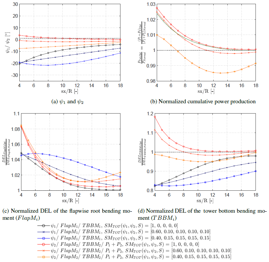
Figure 11Combined load- and power-based optimization with respect to the DEL of the flapwise root bending moment (FlapM) and the DEL of the combined tower bending moment (TBBM) for the upstream and the downstream turbine. The weighting is given as follows: []. The optimization which included the DEL of the upstream and the downstream turbine was done for three cases. The first case is optimizing only for the power which has the weighting SM. The second case is a combined scenario which optimizes for the power and the load with a weighting of SM. The final weighting is SM. Squared symbols: power-driven optimization. Circle symbols: combined load-based optimization. Blue to black: ψ1. Red to orange: ψ2. The optimized cumulative power is normalized by the cumulative power during normal operation, i.e. ψ1=0∘ and ψ2=0∘. The DEL values are normalized per turbine, as the ratio of the optimum DEL and the DEL during normal operation with ψ1=0∘ and ψ2=0∘ for each turbine spacing. Green symbols: normalized cumulative power with ψ1=Opt and ψ2=0∘ to see the effects of downstream yawing.
3.6 Validation
As any simplified model, the surrogates include model errors and uncertainties as previously mentioned and quantified. Figure 12 shows contours of the normalized power output of the upstream and the downstream turbine with respect to ψ1 and ψ2 at a turbine spacing of sx=4R, obtained from the surrogate models with an order of p=3 and p=4. As seen, the contours differ for the two surrogate models, hence the sensitivity is different. However, the optimal region for both ψ1 and ψ2 is comparable in magnitude, where p=4 yields higher gain for ∘. The extend of the surrogate of order p=4 yields a larger region of higher power increase, as well as a secondary local optima for positive upstream yaw angles. However, it should be noted that around this region, the training data for the surrogate models are sparse, and hence the confidence in the model results is lower. For the rest of the validation analysis, the turbine spacing of sx=4R is selected since it provided a high power gain during the optimization of the control strategies.

Figure 12Contour plots of the cumulative power output dependant on the upstream and the downstream yaw angle at sx=4R. The power is normalized by the upstream and downstream turbine at ∘.
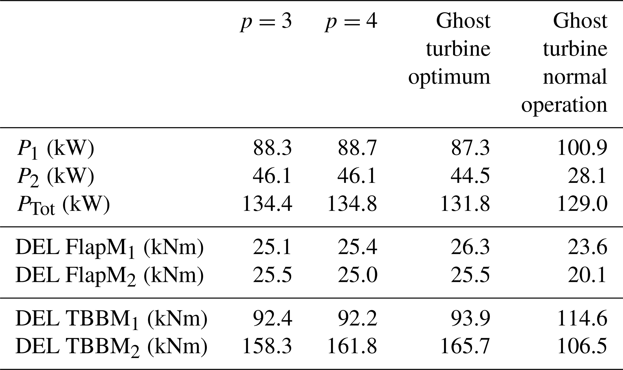
The validation is performed as a blind test via additional simulations in Flex5 with the optimum yaw settings ∘ and ψ2=5.5∘ estimated by the surrogate model of order p=4 at spacing of sx=4R. Table 4 summarizes the results of the surrogate models and the results using the ghost turbines in this Flex5 simulation, which formed the basis for the surrogate models. The surrogate models and the ghost turbines yield very comparable results for the power output, as expected. The surrogate models overestimate the total power output by less than 2 %, which is in agreement with the interpolated surrogate model error in Fig. 10a. Table 4 also verifies the power gain likelihood, ℒ(ΔP) presented in Fig. 10b, where the expected value of true power gain given by the Flex5 simulations is
which is 0.8 % lower than power gain likelihood at 4R downstream reported in Fig. 10b. Note that at this spacing, Fig. 9 shows the expected power gain estimated by the surrogate models p=3 and p=4 as 1.6 % and 3.3 %, respectively. After taking the model bias and difference in 10 min realizations into account, the power gain likelihood of the surrogates is decreased for both p=3 and p=4, approaching the validation values in Table 4. This once again emphasizes the importance and added value of model correction in estimating the true power gain that is likely to be observed in (quasi-)dynamic operation.
The resulting power gain likelihood presented here can be compared to reported gains in literature, where Kheirabadi and Nagamune (2019) have performed a comprehensive review of the reported power gains published across different model fidelities (wind tunnel and field tests). The spread in the reported values is very large, ranging from power loss of −7.9 % to power gains of 46 % for different wind farm layouts and specifications. However, 16 of the 29 examined studies reported power gains in bins ranging from −7.5 % to 12.5 %, so the present results are comparable. Furthermore, it is noteworthy how the majority of the studies using low-fidelity models, e.g. FLORIS, report power gains of approximately 5 % ± 2.5 %, which is comparable to the estimated model error seen in Sect. 3.4.
The equivalent load of the flapwise root bending moment determined with the surrogate model also yields very comparable results with the equivalent loads obtained directly from the Flex5 simulations. There is only a minor difference in the flapwise root bending moments, while the surrogates underestimate the tower bottom bending moment by less than 5 %, which should be accounted for by including the model error.
Table 4Comparison between the power output and the equivalent loads of the surrogate model for the optimal yaw settings (∘ and ψ2=5.5∘) and the normal operation (ψ1=0∘ and ψ2=0∘) at different polynomial orders for the upstream and the downstream turbines at 4R.
EllipSys3D has been used to perform large eddy simulations of a V27 turbine operating at different yaw angles to investigate wake steering. The turbine has been modelled using actuator lines, which are fully coupled to the aeroelastic tool Flex5. The full flow field is extracted at different downstream distances and used as turbulent input to Flex5 to mimic a downstream turbine operating in the deflected wake of an upstream turbine. The upstream turbine has also been modelled with turbulent inflow in Flex5. The performance and response of the two turbines are used to construct surrogate models of different orders based on polynomial chaos expansion.
It is shown how the accuracy of the surrogate models depends on the amount of training data, and how the choice of order for the polynomials needs to be considered to capture more complexity but also to avoid overfitting. The constructed surrogate models consistently yield median errors for a variety of control inputs, i.e. the yaw angles of the upstream and downstream turbines at different turbine spacings. Considering the entire domain of the optimization, the surrogate models consistently overestimate the power output of the downstream turbine by approximately 2 % for most turbine spacings. The performance of FLORIS is also compared to the high-fidelity results for different control settings. FLORIS yields very large relative errors for close turbine spacings and moderately wide, biased distributions for larger turbine spacings, with median errors of 5 % and 3 % standard deviation for the investigated configuration.
Due to their higher accuracy, the surrogate models are used to optimize the power production. The two surrogate models of order 3 and 4 generally show similar results in terms of cumulative power production of the two turbines. However, the power gain optimized using surrogate models with p=3 and p=4 are very different for small turbine spacings due to the difference in the inherit model error and uncertainties. The model error was estimated to be small (<1 %) but with significant standard deviation in the model error of ±2 %. The optimization results were furthermore corrected by the estimated model error to give a power gain likelihood, i.e. the most realistic optimization performance when correcting for model error and known uncertainties. However, uncertainties originated from the inherent variability of the inflow, and the induction is not accounted for. The optimized power gain likelihood showed a potential for improving the power production by almost 3 % ± 1 % for turbine spacings less than 7R. The optimized power gain likelihood decreased to 0 % for larger turbine spacing as the optimization resulted in only minor or no yaw of the turbines, i.e. converging to normal operation as attempting to wake steer becomes unfavourable. The associated uncertainty is significant, and the comparison between power gain estimated directly by the surrogate models and the corrected power gain likelihood emphasize the need to correct model results and take the uncertainties into consideration. In other words, the uncertainty of the model outputs and control inputs has to be considered in order to assess the true performance of the wind farm control strategies and to decide whether to apply a given control strategy. All uncertainties considered, it might therefore not be sensible to apply wake steering for the current turbine and flow scenario, unless the two turbines are very closely spaced.
A combination of surrogate models has also been used to include the DEL in the optimization. The results showed that it is possible to reduce the tower bottom bending moments for both turbines by sacrificing some of the power gain. On the other hand, it is generally not possible to reduce the flapwise root bending moments. The combined power and load optimization also generally converge to normal operation with no yawing of the two turbines for larger spacings.
Finally, the optimization results were compared and validated against additional Flex5 simulation at the optimum yaw angles predicted by the surrogates. The validation confirmed the power gain likelihood assessment and provided estimates of the DEL of both flapwise root and tower bottom bending moments, which were underpredicted by less than 5 %.
The surrogate approach used in this study could be extended in several ways. To be generally applicable it should include different flow cases, e.g. wind speed, turbulence intensity, shear, and atmospheric stability. The surrogates can also be expanded by including field measurements when available. Additional surrogate models can be constructed for other turbine models. The true performance test of the presented optimization procedure should be conducted in a wind farm environment, where the flow complexity would increase and hence also the requirements on the model corrections and uncertainty estimations.
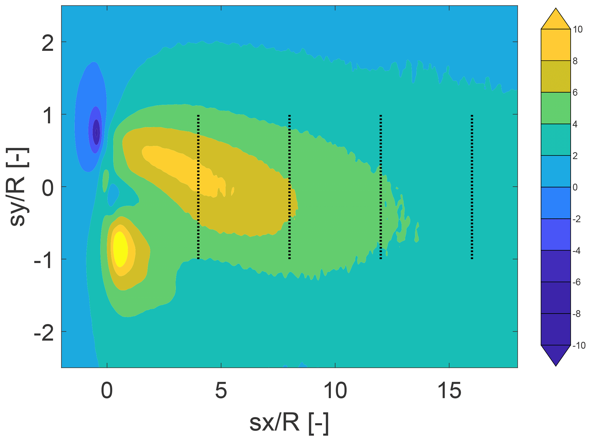
Figure A1Averaged horizontal scan of the flow angle obtained with the coupling between EllipSys3D and Flex5 at ∘ at hub height. The average flow angle over the rotor area at is 6.4∘, 5.3∘, 3.8∘ and 3.2∘. The dotted black lines indicate the rotor area.
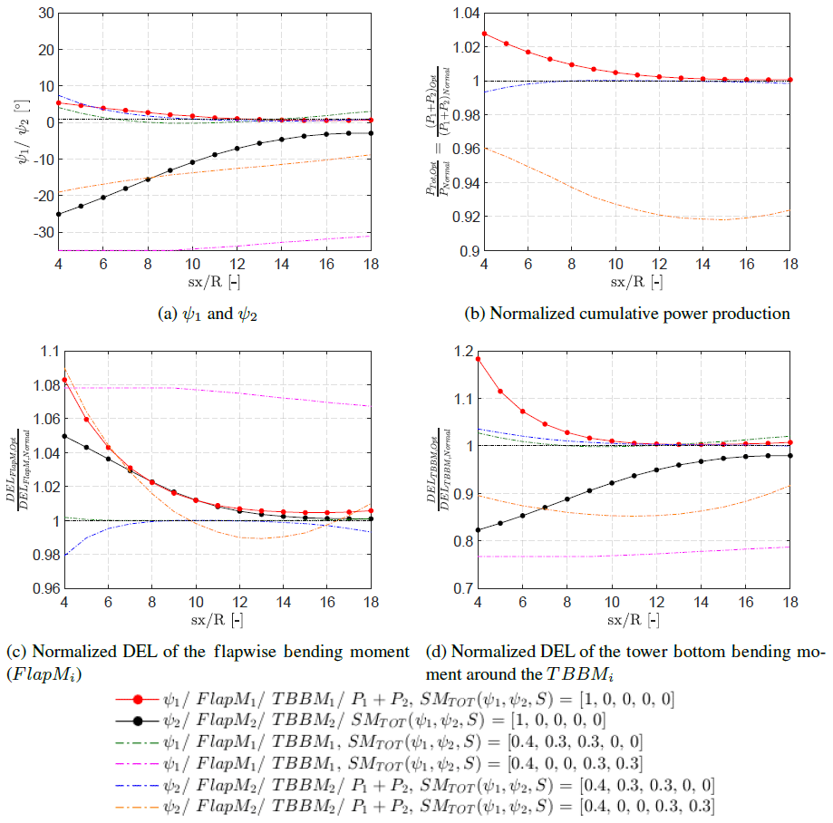
Figure B1Combined load- and power-based optimization with respect to the DEL of the flapwise root bending moment (FlapM) and the DEL of the combined tower bending moment (TBBM) for the upstream and the downstream turbines. The weighting is given as follows: []. The optimization which included the DEL of the upstream and the downstream turbines was done for two additional cases. The first case is a combined scenario which optimizes for the power and the load with a weighting of SM. The second case has a weighting of SM. Red and black symbols: power-driven optimization. Green and magenta dashed line: first combined load- and power-based optimization. Blue and orange dashed line: second combined load- and power-based optimization. The optimized cumulative power is normalized by the cumulative power during normal operation, i.e. ψ1=0∘ and ψ2=0∘. The DEL values are normalized per turbine, as the ratio of the optimum DEL and the DEL during normal operation with ψ1=0∘ and ψ2=0∘ for each turbine spacing.
| AEP | Annual energy production |
| AL | Actuator line |
| BEM | Blade element momentum |
| CFD | Computational fluid dynamics |
| DEL | Damage equivalent load |
| FlapM | Flapwise root bending moment |
| FLORIS | FLOw Redirection and Induction in Steady State |
| LES | Large eddy simulation |
| NREL | National Renewable Energy Laboratory |
| PCE | Polynomial chaos expansion |
| QUICK | Quadratic Upstream Interpolation for Convective Kinematics |
| SM | Surrogate model |
| SWiFT | Scaled Wind Farm Technology |
| TBBM | Total tower bottom bending moment |
| TI | Turbulence intensity |
The input data and surrogate model data are available at https://github.com/Paul1994H/Surrogates-Wind-Farm-Control-Model.git (Hulsman, 2019).
LES was performed by SJA, while the initial analysis was done by PH. All authors contributed to the extended analysis and reporting.
The authors declare that they have no conflict of interest.
The authors also wish to thank Nikolay Krasimirov Dimitrov for fruitful discussions on the polynomial chaos expansion theory. The study is partially supported by the CONCERT Project (Project no. 2016-1-12396), funded by Energinet.dk under the Public Service Obligation (PSO) and the CCA on Virtual Atmosphere.
This research has been supported by the Energinet.dk (grant no. 2016-1-12396).
This paper was edited by Athanasios Kolios and reviewed by two anonymous referees.
Anderson, M.: Horizontal axis wind turbines in yaw, in: Wind Energy Workshop, 57–67, Multi-Science Publishing, Proceedings of the First BWEA Wind Energy Workshop, 1979. a
Annoni, J., Fleming, P., Scholbrock, A., Roadman, J., Dana, S., Adcock, C., Porte-Agel, F., Raach, S., Haizmann, F., and Schlipf, D.: Analysis of control-oriented wake modeling tools using lidar field results, Wind Energ. Sci., 3, 819–831, https://doi.org/10.5194/wes-3-819-2018, 2018. a, b, c
Bartl, J., Mühle, F., Schottler, J., Sætran, L., Peinke, J., Adaramola, M., and Hölling, M.: Wind tunnel experiments on wind turbine wakes in yaw: effects of inflow turbulence and shear, Wind Energ. Sci., 3, 329–343, https://doi.org/10.5194/wes-3-329-2018, 2018a. a
Bartl, J., Mühle, F., and Sætran, L.: Wind tunnel study on power output and yaw moments for two yaw-controlled model wind turbines, Wind Energ. Sci., 3, 489–502, https://doi.org/10.5194/wes-3-489-2018, 2018b. a
Bastankhah, M. and Porté-Agel, F.: A new analytical model for wind-turbine wakes, Renew. Energ., 70, 116–123, 2014. a
Bastankhah, M. and Porté-Agel, F.: Experimental and theoretical study of wind turbine wakes in yawed conditions, J. Fluid Mech., 806, 506–541, 2016. a, b, c, d
Branlard, E: Wind turbine aerodynamics and vorticity-based methods, Vol. 10, New York, Springer, 2017. a
Dimitrov, N., Kelly, M. C., Vignaroli, A., and Berg, J.: From wind to loads: wind turbine site-specific load estimation with surrogate models trained on high-fidelity load databases, Wind Energ. Sci., 3, 767–790, https://doi.org/10.5194/wes-3-767-2018, 2018. a
Feinberg, J. and Langtangen, H. P.: Chaospy: An open source tool for designing methods of uncertainty quantification, J. Comput. Sci., 11, 46–57, 2015. a, b
Fleming, P., Annoni, J., Churchfield, M., Martinez-Tossas, L. A., Gruchalla, K., Lawson, M., and Moriarty, P.: A simulation study demonstrating the importance of large-scale trailing vortices in wake steering, Wind Energ. Sci., 3, 243–255, https://doi.org/10.5194/wes-3-243-2018, 2018. a
Fleming, P. A., Gebraad, P. M., Lee, S., van Wingerden, J.-W., Johnson, K., Churchfield, M., Michalakes, J., Spalart, P., and Moriarty, P.: Evaluating techniques for redirecting turbine wakes using SOWFA, Renew. Energ., 70, 211–218, 2014. a
Fleming, P. A., Ning, A., Gebraad, P. M., and Dykes, K.: Wind plant system engineering through optimization of layout and yaw control, Wind Energy, 19, 329–344, 2016. a
Gaumond, M., Réthoré, P. E., Ott, S., Peña, A., Bechmann, A., and Hansen, K. S.: Evaluation of the wind direction uncertainty and its impact on wake modeling at the Horns Rev offshore wind farm, Wind Energy, 17, 1169–1178, https://doi.org/10.1002/we.1625, 2014. a
Gebraad, P., Teeuwisse, F., Wingerden, J., Fleming, P. A., Ruben, S., Marden, J., and Pao, L.: Wind plant power optimization through yaw control using a parametric model for wake effects – a CFD simulation study, Wind Energy, 19, 95–114, 2016. a
Gebraad, P., Thomas, J. J., Ning, A., Fleming, P., and Dykes, K.: Maximization of the annual energy production of wind power plants by optimization of layout and yaw-based wake control, Wind Energy, 20, 97–107, 2017. a, b
Gebraad, P. M. and Van Wingerden, J.: A control-oriented dynamic model for wakes in wind plants, J. Phys. Conf. Ser., 524, 012186, https://doi.org/10.1088/1742-6596/524/1/012186, 2014. a
Gilling, L., Sørensen, N. N., and Réthoré, P.-E.: Imposing resolved turbulence by an actuator in a detached eddy simulation of an airfoil, EWEC, European Wind Energy Conference and Exhibition – Marseille, France, 2009. a
Hasager, C., Nygaard, N., Volker, P., Karagali, I., Andersen, S., and Badger, J.: Wind Farm Wake: The 2016 Horns Rev Photo Case, Energies, 10, 317, https://doi.org/10.3390/en10030317, 2017. a
Hulsman, P.: PCE surrogates for power and loads under wind farm control, available at: https://github.com/Paul1994H/Surrogates-Wind-Farm-Control-Model.git, last access: 13 November 2019. a
Jiménez, Á., Crespo, A., and Migoya, E.: Application of a LES technique to characterize the wake deflection of a wind turbine in yaw, Wind Energy, 13, 559–572, 2010. a
Kheirabadi, A. C. and Nagamune, R.: A quantitative review of wind farm control with the objective of wind farm power maximization, J. Wind Eng. Ind. Aerod., 192, 45–73, https://doi.org/10.1016/j.jweia.2019.06.015, 2019. a
Knudsen, T., Bak, T., and Svenstrup, M.: Survey of wind farm control–power and fatigue optimization, Wind Energy, 18, 1333–1351, 2015. a
Kragh, K. A. and Hansen, M. H.: Potential of power gain with improved yaw alignment, Wind Energy, 18, 979–989, 2015. a
Leonard, B. P.: A stable and accurate convective modelling procedure based on quadratic upstream interpolation, Comput. Method. Appl. M., 19, 59–98, 1979. a
Liew, J., Urbán, A. M., and Andersen, S. J.: Analytical model for the power-yaw sensitivity of wind turbines operating in full wake, Wind Energ. Sci. Discuss., https://doi.org/10.5194/wes-2019-65, in review, 2019. a
Mann, J.: The spatial structure of neutral atmospheric surface-layer turbulence, J. Fluid Mech., 273, 141–168, 1994. a
Mann, J.: Wind field simulation, Probabilist. Eng. Mech., 13, 269–282, 1998. a
Mann, J., Peña, A., Troldborg, N., and Andersen, S. J.: How does turbulence change approaching a rotor?, Wind Energ. Sci., 3, 293–300, https://doi.org/10.5194/wes-3-293-2018, 2018. a
Martínez-Tossas, L. A., Annoni, J., Fleming, P. A., and Churchfield, M. J.: The aerodynamics of the curled wake: a simplified model in view of flow control, Wind Energ. Sci., 4, 127–138, https://doi.org/10.5194/wes-4-127-2019, 2019. a
McKay, P., Carriveau, R., and Ting, D. S.-K.: Wake impacts on downstream wind turbine performance and yaw alignment, Wind Energy, 16, 221–234, https://doi.org/10.1002/we.544, 2013. a
Medici, D. and Alfredsson, P.: Measurements on a wind turbine wake: 3D effects and bluff body vortex shedding, Wind Energy, 9, 219–236, 2006. a
Medici, D. and Dahlberg, J.: Potential improvement of wind turbine array efficiency by active wake control (AWC), Proceedings of European Wind Energy Conference, Madrid, 2003. a
Michelsen, J. A.: Basis3D-a platform for development of multiblock PDE solvers, Tech. rep., Technical Report AFM 92-05, PhD thesis, Technical University of Denmark, Lyngby, 1992. a
Mikkelsen, R.: Actuator disc methods applied to wind turbines, PhD thesis, Technical University of Denmark, Lyngby, 2003. a
Mittelmeier, N. and Kühn, M.: Determination of optimal wind turbine alignment into the wind and detection of alignment changes with SCADA data, Wind Energ. Sci., 3, 395–408, https://doi.org/10.5194/wes-3-395-2018, 2018. a
Murcia, J. P., Réthoré, P.-E., Dimitrov, N., Natarajan, A., Sørensen, J. D., Graf, P., and Kim, T.: Uncertainty propagation through an aeroelastic wind turbine model using polynomial surrogates, Renew. Energ., 119, 910–922, 2018. a
Øye, S.: FLEX4 simulation of wind turbine dynamics, in: Proceedings of the 28th IEA Meeting of Experts Concerning State of the Art of Aeroelastic Codes for Wind Turbine Calculations (available through International Energy Agency), Technical University of Denmark, Lyngby, 1996. a
Quick, J., Annoni, J., King, R., Dykes, K., Fleming, P., and Ning, A.: Optimization Under Uncertainty for Wake Steering Strategies, J. Phys. Conf. Ser., 854, 012036, https://doi.org/10.1088/1742-6596/854/1/012036, 2017. a
Resor, B. and LeBlanc, B.: An Aeroelastic Reference Model for the SWIFT Turbines, Sandia National Laboratories, Albuquerque, NM, USA, 2014. a, b, c
Ribner, H. S.: Propellers in yaw, NASA, Advance Restricted Report 3L09, NACA Wartime Report L-219, Langley Field, VA, USA, 1943. a
Smulders, P. T., Lenssen, G., and van Leeuwen, H.: Experiments with windrotors in yaw, Technische Hogeschool, Afdeling der Technische Natuurkunde, Vakgroep Transportfysica, Proceedings of the International Symposium on Envi- ronmental Problems, Patras, Greece, 1981. a
Sørensen, J. N. and Shen, W. Z.: Numerical modeling of wind turbine wakes, J. Fluids Eng., 124, 393–399, 2002. a
Sørensen, J. N., Mikkelsen, R. F., Henningson, D. S., Ivanell, S., Sarmast, S., and Andersen, S. J.: Simulation of wind turbine wakes using the actuator line technique, Philos. T. R. Soc. A, 373, 20140071, https://doi.org/10.1098/rsta.2014.0071, 2015. a
Sørensen, N. N.: General purpose flow solver applied to flow over hills, Risø National Laboratory, Risø, 1995. a
Sudret, B.: Global sensitivity analysis using polynomial chaos expansions, Reliab. Eng. Syst. Safe., 93, 964–979, 2008. a
Troldborg, N.: Actuator line modeling of wind turbine wakes, PhD thesis, Technical University of Denmark, Lyngby, 2009. a
Troldborg, N. and Meyer Forsting, A. R.: A simple model of the wind turbine induction zone derived from numerical simulations, Wind Energy, 20, 2011–2020, 2017. a
Troldborg, N., Sørensen, J. N., Mikkelsen, R., and Sørensen, N. N.: A simple atmospheric boundary layer model applied to large eddy simulations of wind turbine wakes, Wind Energy, 17, 657–669, 2014. a
van Dijk, M. T., van Wingerden, J.-W., Ashuri, T., Li, Y., and Rotea, M. A.: Yaw-Misalignment and its Impact on Wind Turbine Loads and Wind Farm Power Output, J. Phys. Conf. Ser., 753, 062013, https://doi.org/10.1088/1742-6596/753/6/062013, 2016. a
Ziegler, L., Gonzalez, E., Rubert, T., Smolka, U., and Melero, J. J.: Lifetime extension of onshore wind turbines: A review covering Germany, Spain, Denmark, and the UK, Renew. Sust. Energ. Rev., 82, 1261–1271, https://doi.org/10.1016/j.rser.2017.09.100, 2018. a
The python code of the FLORIS model was obtained from GitHub and version 0.1.1 was used (https://github.com/WISDEM/FLORIS, last access: 11 June 2018).
- Abstract
- Introduction
- Methodology
- Results
- Conclusion
- Appendix A: Wake inflow direction
- Appendix B: Additional load- and power-based optimization
- Appendix C: Nomenclature
- Code and data availability
- Author contributions
- Competing interests
- Acknowledgements
- Financial support
- Review statement
- References