the Creative Commons Attribution 4.0 License.
the Creative Commons Attribution 4.0 License.
 | 31 Mar 2020
Analytical model for the power–yaw sensitivity of wind turbines operating in full wake
Albert M. Urbán
Søren Juhl Andersen
Wind turbines are designed to align themselves with the incoming wind direction. However, turbines often experience unintentional yaw misalignment, which can significantly reduce the power production. The unintentional yaw misalignment increases for turbines operating in the wake of upstream turbines. Here, the combined effects of wakes and yaw misalignment are investigated, with a focus on the resulting reduction in power production. A model is developed, which considers the trajectory of each turbine blade element as it passes through the wake inflow in order to determine a power–yaw loss exponent. The simple model is verified using the HAWC2 aeroelastic code, where wake flow fields have been generated using both medium- and high-fidelity computational fluid dynamics simulations. It is demonstrated that the spatial variation in the incoming wind field, due to the presence of wakes, plays a significant role in the power loss due to yaw misalignment. Results show that disregarding these effects on the power–yaw loss exponent can yield a 3.5 % overestimation in the power production of a turbine misaligned by 30∘. The presented analysis and model is relevant to low-fidelity wind farm optimization tools, which aim to capture the combined effects of wakes and yaw misalignment as well as the uncertainty on power output.
- Article
(1048 KB) - Full-text XML
- BibTeX
- EndNote


As the global wind energy sector continues to grow, there is a strong demand for a decreased levelized cost of energy. With this demand comes an increasing need for accurate and efficient computational tools, which are able to improve the design of wind farms and optimize annual energy production. In the early phases of wind farm design, optimization tools provide estimates of energy production and the costs during construction, installation, and operation. The wind farm planning tools must account for the interactions between nearby wind turbines using wake models. Often, the wake effects and, therefore, the power production are not accurately modeled when employing engineering wake models, and they include substantial uncertainty; see e.g., Nygaard (2015) and Peña et al. (2018). Unintentional yaw misalignment (or yaw error) of turbines inside wind farms occurs frequently, which can partially explain the discrepancy and uncertainty. For example, Mikkelsen et al. (2010) reported yaw errors on a turbine in free-stream wind conditions of up to 20∘ during a 3 h measurement campaign. McKay et al. (2013) have shown yaw misalignment of up to 35∘ for turbines operating in the wakes of aligned upstream turbines based on field measurements for a 6-month period. Furthermore, it was shown that the yaw misalignment was accentuated further downstream for turbines affected by multiple wakes. The probability of a turbine affected by wakes to be yaw misaligned ±25∘ was more than 25 %.
Wind turbines which experience yaw misalignment show a reduction in power production. This power sensitivity to yaw misalignment can be quantified by the power–yaw loss exponent, α, which is found in the expression
where γ is the yaw misalignment angle between the turbine rotor and the local wind direction, and Pγ is the power generated by a wind turbine with a yaw misalignment of γ. P0 is the power generated when the turbine experiences no yaw misalignment. Numerous values of the power–yaw loss exponent, α, have been proposed in literature. Based on blade element momentum (BEM) theory, it is commonly concluded that α=3. However, experimental results have often shown that this value overestimates the power loss due to yaw (Aagaard Madsen et al., 2003). Schepers (2001) found experimentally that α=1.8, and Dahlberg and Montgomerie (2005) found a range between α=1.88 and α=5.14. Gebraad et al. (2016) use a constant α=1.88, determined by using the wind farm simulator, SOWFA (Fleming et al., 2013). Medici (2005) found a value of α=2 from wind tunnel data. However, these considerations are simplified and only valid for free-stream conditions.
The investigation performed by Urbán et al. (2019) shows that yaw misalignment of a turbine in the wake of another turbine can exhibit significant variations in the power–yaw loss exponent. In particular, α depends on the shape of the wake deficit profile, which evolves as it propagates downstream. The wake recovery rate is highly dependent on turbine spacing and ambient turbulence intensity. It was found that α is maximum for a turbine located approximately four rotor diameters (4D) downstream of another turbine when in a full-wake situation. Furthermore, α tends to decrease rapidly as turbine spacing decreases below 4D, while α converges slowly to a fixed value as turbine spacing increases.
Considering the findings in McKay et al. (2013), the implication of unintentional yaw misalignment can be significant for the total power production of large wind farms. Efforts to reduce the yaw error include improved measuring techniques for individual turbine control (e.g., Kragh et al., 2013; Schlipf et al., 2013), as well as farm level control, where the information on wind direction is shared between turbines in close proximity to improve the overall alignment (see Annoni et al., 2019). However, it should be mentioned that part of the yaw misalignment compared to the free-stream wind direction should not necessarily be considered a yaw error. The turbine attempts to align itself with the local inflow direction to optimize the power production, where the presence of wake effects may alter the local flow wind direction. Such behavior was also described by McKay et al. (2013) and shown experimentally by Bartl et al. (2018) as well as through the use of surrogate models based on high-fidelity simulations in Hulsman et al. (2019), where the second turbine should indeed align itself with the local wind direction to optimize power production. Archer and Vasel-Be-Hagh (2019) used large-eddy simulations (LESs) to also show how turbines deep inside the farm could be intentionally yawed for improved performance.
In recent years, there has been an increased focus on applying control strategies for both stand-alone wind turbines and entire wind farms to increase operational performance. The focus is generally on power optimization, for example, Knudsen et al. (2015) and Gebraad et al. (2015). A common form of wind farm control for power optimization is wake steering, in which a wake can be redirected away from a downstream turbine by inducing a yaw misalignment in the upstream turbine. Numerous studies on wake redirection have been performed by Fleming et al. (2016), Gebraad et al. (2016), Gebraad et al. (2017), Jiménez et al. (2010), Bossanyi (2018), and Munters and Meyers (2018), showing improved annual energy production in wind farms ranging between 2 % and 8 %. These investigations often assume a constant value of α to determine the trade-off between power losses due to yawing the upstream turbine and the power gain of the downstream turbine. An exception to this can be found in the study by Munters and Meyers (2018), who modeled the turbines as actuator disks which could yaw, and that by Bossanyi (2018), where α is adjusted based on the blade pitch angle of the yawed turbine. Overlooking the causes and effects of a varying power–yaw loss exponent becomes a problem in the framework of low-fidelity wind farm optimization, where the layout of the wind farm itself can change the values of α for each turbine. For example, both Gebraad et al. (2017) and Howland et al. (2019) demonstrate potential power increases in a wind farm by performing wake steering, where the analysis relies on a constant α despite the fact that some turbines are yawed in wake situations. It is beneficial to further investigate the behavior of α in order to better predict the trade-off of yaw steering, especially in the event that a turbine is yawed when operating in the wake of another turbine. The estimates of these power losses could benefit from a more accurate estimation of α by taking into account the increased uncertainty of yaw alignment when a turbine is in a wake.
By overcoming the assumption of a constant power–yaw loss exponent, uncertainty in wind farm modeling tools can be decreased. Low-fidelity wind farm optimization frameworks such as TOPFARM (Réthoré et al., 2014), FLORIS (Fleming et al., 2018), or FarmFlow (Soleimanzadeh et al., 2012) could benefit from including the presented model for estimating α, allowing for more accurate results. This paper focuses on the estimation of power loss of a wind turbine when yawed in wake and aims to extend the work of Urbán et al. (2019), who used the dynamic wake meandering (DWM) model in conjunction with the aeroelastic tool, HAWC2, to study the effects of axisymmetric wake profiles on a misaligned wind turbine. In the presented work, the DWM-generated wakes are validated against wakes generated by large-eddy simulations (LESs). Furthermore, an analytical formulation, based on concepts of blade element momentum (BEM) theory, is presented, which captures the behavior of α in axisymmetric wake situations. The analytical formulation is able to estimate values of α rapidly, without the need for aeroelastic simulations. The calculation of α for a range of turbine spacings can be performed in a few seconds, whereas aeroelastic simulations performing the same task require a time frame on the order of hours. The analytical formulation is validated against simulations using HAWC2, an aeroelastic code which uses an unsteady BEM induction model for nonuniform inflow conditions (Madsen et al., 2019). The HAWC2 simulations are used in conjunction with both the DWM model and LES to generate the dynamic wake inflow. The presented analytical model can be used in existing wind farm optimization frameworks as a power correction for misaligned wind turbines in full-wake scenarios.
When a downstream turbine in a full-wake situation is perfectly aligned with the incoming wind, each blade segment follows a circular trajectory relative to the mean incoming wind direction. For misaligned cases, where the turbine is yawed, each blade segment follows an elliptical path, where the eccentricity of the ellipse increases with yaw angle (Fig. 1a). When these trajectories are plotted on an unfolded polar grid (Fig. 1b), it can be observed that the blade segment passes through different regions of the wake inflow. As the yaw angle increases, all blade segments on a rotor experience flow near the wake center for an increasing period of time. This suggests that the spatial distribution of the wake profile could have an effect on how the power output of a turbine changes with yaw angle. It is therefore proposed that the power output contribution of each blade segment depends on the average wind speed experienced as a result of following a trajectory through a nonuniform wind field. It is convenient to define a transformation between rotor coordinates (rR, ψR) and meteorological coordinates (rm, ψm), where r and ψ are the radial position and azimuth angle, respectively. The transformation is based on the definition of an ellipse:
where the semimajor and semiminor axes of the ellipse are rR and rRcos (ψ), respectively, and the eccentricity is sin (γ).
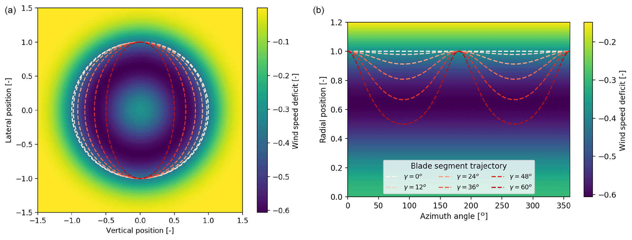
Figure 1The trajectory of a blade segment close to the blade tip through a wake inflow at varying yaw angles, represented in Cartesian coordinates (a) and unfolded polar coordinates (b). Distances and wind speeds are normalized by rotor radius, R, and free wind speed, U0, respectively (generated using DWM, U=10 m s−1, x=3D).
2.1 Blade segment effective wind speed in an axisymmetric wake
This section introduces the concept of blade segment effective wind speed. For a blade segment located at radius, rR, the blade segment effective wind speed, , is defined as the expected value of wind speed experienced by the blade segment as it follows a trajectory through the wind field:
where 𝔼[.] is the expected value function, and U(rm) is assumed to be axisymmetric as displayed in Fig. 1 and is therefore only a function of radius in meteorological coordinates. One way of expressing Eq. (3), assuming the blade segment trajectory is an ellipse as described in Fig. 1, is (see Lemma A1 in Appendix A)
where is the cumulative density function of rm from Eq. (2) (see Lemma A2 in Appendix A):
From the formulation in Eq. (4), it can be observed that the blade segment effective wind speed consists of two additive components. The uniform velocity depends on the wind speed at the rotor radius, whereas an added velocity component depends on radial variations (dU∕dr) in the wind field. In a uniform wind field, where , the blade segment effective wind speed remains unchanged when the turbine is yawed. In a nonuniform wind field, the sign of dU∕dr determines if the added velocity provides a surplus or a deficit to the blade segment effective wind speed. For instance, Fig. 2 shows the radial variation in the wind speed and its derivative for different downstream positions in a wake generated by the DWM model. When the radial wind field function decreases with radius (), such as in the near wake, the blade segment effective wind speed increases. The opposite occurs when the radial wind field function increases with radius. Therefore, given U(rm), it is possible to explicitly calculate given a value of γ and rR by solving Eq. (4).
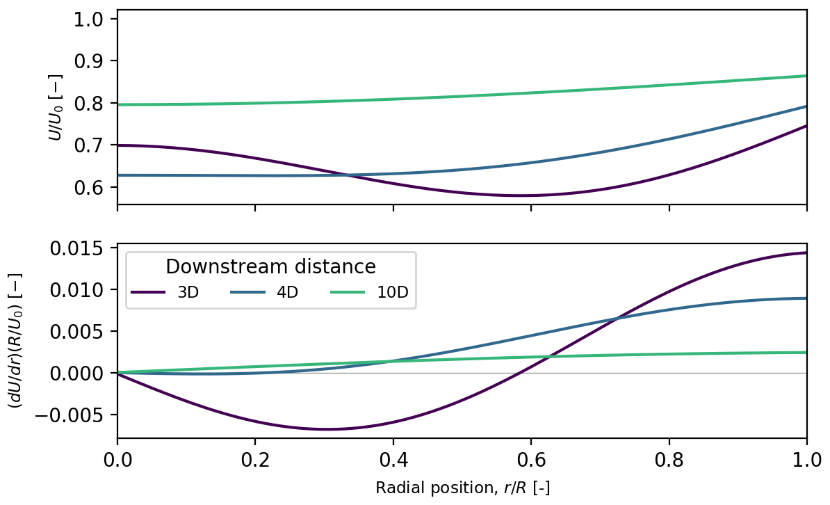
Figure 2Radial functions of wind speed deficit and its derivative for varying turbine spacing distances (generated using DWM, D=96.2 m).
2.2 Modified BEM formulation of wind turbine power in steady yaw and axisymmetric wake
Based on blade element momentum (BEM) theory,
where is assumed to be constant, where ρ is the density of air and a is the axial induction. In order to stay consistent with the definition of α in Eq. (1), as well as the assumption that each blade segment experiences a blade segment effective wind speed, it is proposed that Eq. (6) is modified to
where α0 is the power–yaw loss exponent from Eq. (1) for a turbine in free-stream conditions. Integrating Eq. (7) over the length of the blade gives the total power output of the turbine:
Therefore the power ratio defined on the left-hand side of Eq. (1) is
It is therefore possible to determine a value of α from Eq. (1) which best fits Eq. (9) using curve fitting methods. This is achieved in this investigation using a least-squares optimization:
where Pγ|x is the power output of a turbine for a yaw misalignment, γ, and a turbine spacing, x. This analytical approximation of α gives an estimate for a turbine's power sensitivity to yawing while in full-wake conditions. The inclusion of α0 in Eq. (9) ensures Pγ∕P0 converges to the free-stream value as turbine spacing becomes large and wake effects dissipate. Additionally, if the turbine faces a uniform wind field, then α=α0.
To determine the value of α for varying turbine spacing, four methods are used to estimate the relative power production when a turbine is yawed in a wake situation: (1) aeroelastic simulations with DWM-generated wakes, (2) aeroelastic simulations with LES-generated wakes, (3) analytical models with DWM-generated wakes, and (4) analytical models with LES-generated wakes.
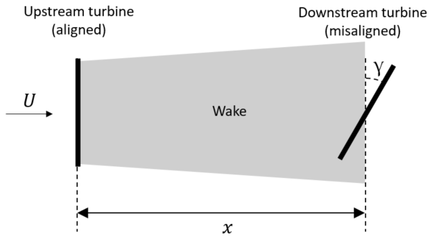
The aeroelastic simulations are used to validate the results produced by the analytical model. Additionally, the inclusion of LES-generated wakes in this investigation verifies the results of the DWM-generated wake, which is unable to capture the behavior of a wake in as much detail as LES. Each of the model–simulation combinations aims to determine the power output Pγ|x of the downstream wind turbine with yaw misalignment of γ in the full wake of an upstream turbine located at a distance, x, apart as illustrated in Fig. 3.
To ensure that the combination of wake generation and simulation tools produces comparable results, the free-stream wind speed is fixed at 8 m s−1 with an ambient turbulence intensity of 6 % and a shear exponent of 0.14. The free variables, x and γ, are varied over the ranges of 3D to 14D and −30 to 30∘, respectively. The α exponent is determined for each turbine spacing distance for the four model–calculation combinations by performing the curve fitting in accordance with the definition of α in Eq. (1).
3.1 Aeroelastic simulation
The aeroelastic simulations (1) and (2) are run using the aeroelastic code HAWC2 (Larsen and Hansen, 2007) using a 2.3 MW turbine with a diameter of 96.2 m and operating in full wake. The wake-generating turbine is similar and has a fixed rotor speed of 1.37 rad s−1 and blade pitch angle of −1∘ to reflect the mean operating conditions at 8 m s−1, which was previously obtained based on the flow conditions defined below. Simulation (1) uses the DWM model to generate the wake on the target turbine as performed in Urbán et al. (2019). Simulation (2) uses a LES-generated wake as the input wind field for the aeroelastic simulations which include the wake dynamics. From the simulations, the mean power output is obtained for different turbine spacings and misalignment angles. The results are used to calculate the power–yaw loss exponent for each turbine spacing using Eq. (10).
3.1.1 DWM-generated wake
The dynamic wake meandering model, as described by Larsen et al. (2008), is used in combination with HAWC2. The DWM model unifies three key components of wake generation in a computationally efficient manner. These components are the wake deficit profile, the added turbulence profile, and wake meandering. The DWM model produces an axisymmetric wake profile for each downstream distance using the thrust properties of the upstream turbine. Added wake turbulence is superimposed over the wake profile, and the axisymmetric wake profile is translated to mimic the effects of wake meandering as described in Madsen et al. (2010) and shown in Fig. 4e. The implementation of the DWM model in HAWC2 has been validated against field data in Larsen et al. (2013). Additionally, a steady variation in the DWM model used in Sect. 3.2.1 has been validated in Keck (2015).
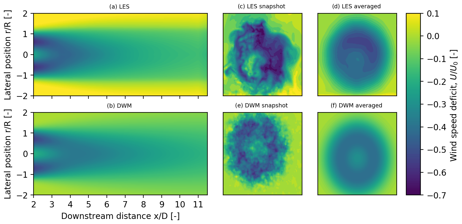
Figure 4Visualizations of the LES and DWM wakes represented as the averaged wake downstream evolution (a, b), wake profile snapshots at x=3D (c, e), and wake-averaged wake profiles at x=3D (d, f).
3.1.2 LES-generated wake
The turbine and its wake are simulated using the incompressible Navier–Stokes solver EllipSys3D coupled with the aeroelastic tool Flex5 through the actuator line method. EllipSys3D is based on a finite-volume approach with general curvilinear coordinates (Michelsen, 1992; Sørensen, 1995). The actuator line method as developed by Sørensen and Shen (2002) applies body forces along rotating lines to simulate the presence of the turbine within the flow domain. The position of the rotating lines and applied body forces are determined through the aeroelastic tool Flex5 by Øye (1996), which gives forces and deflections of the turbine. The effects of atmospheric boundary layer and inflow turbulence are also included using body forces. The atmospheric boundary layer is modeled with a shear exponent of 0.14. The inflow turbulence is generated using a Mann box (Mann, 1994, 1998). The boxes are generated using the following inputs. , where ϕ is the spectral Kolmogorov constant1 and ϵ is the specific rate of turbulent dissipation. Additionally, a turbulent length scale L=50, and Γ=3.2, which describes the anisotropy of the generated turbulence, are used. These parameters result in a turbulence intensity of approximately 6 %. For additional details on the numerical framework, please see Sørensen et al. (2015). The turbine and its wake are simulated in a domain of in the lateral, vertical, and streamwise directions. The turbine is placed at (5D, 0.6865D, 5.5D) and each blade is resolved by 27 cells. The wind fields consisting of all three velocity components are extracted for every 0.5D in the wake behind the turbine. These flow fields are used as input to HAWC2 and compared to the wind fields generated using the DWM model as described previously. The wake profiles extracted from the LES framework are expected to be more realistic given that they include the asymmetric effects of shear on the wake as well as the nonlinear interactions in a dynamic wake inherent to the flow. These effects are visualized in Fig. 4c, where the asymmetry and different turbulent structures are more realistic compared the DWM model in Fig. 4e.
3.2 Analytical calculation
Simulations (3) and (4) are performed using the wake profiles generated by a stand-alone version of the DWM model and the time-averaged LES wake deficit profiles, as well as the analytical formulation described in Sect. 2. The radial wind function, U(r), is extracted from the wake profiles for varying turbine spacing, shown in Fig. 4a and b. Equations (4) and (9) are solved using numerical differentiation and integration techniques, and the α fit is determined using Eq. (10).
3.2.1 DWM-generated wake
The DWM model, originally coded within HAWC2, has been externalized for its use within optimization problems, which results in fast and accurate estimations of a wake profile for a given radial thrust distribution, ambient turbulence intensity, and turbine spacing (DTU Wind Energy, 2019). A steady wake profile, UDWM(r), is obtained directly from the DWM code. To take into account meandering, UDWM(r) is adjusted by applying a Gaussian smearing using a similar method to Keck (2015), where the spread of the Gaussian captures the standard deviation of the wake meandering motion:
where * is the linear convolution operator. Through a parametric study using the HAWC2 DWM model, the relation σ=1.493x was found to fit best when describing the standard deviation of the wake meandering path. As a result, an axisymmetric, time-invariant wake profile is produced (Fig. 4f), which is used in the analytical model.
3.2.2 LES-generated wake
The wake wind field is preconditioned before being used in the analytical formulation by removing the shear profile. This is achieved by subtracting the mean wind field 1D upstream of the wake-generating turbine from the downstream wind field.
Unlike the DWM model, which fully describes the radial wind function, the LES wake at a particular downstream distance is described as a time-varying two-dimensional wind field, f(x, y, t). The mean radial wind speed function is calculated by performing an azimuthal average as
where N is the number of time steps in the LES wind field, and M is the desired azimuthal discretization (in this case, M=500). The time-averaged and azimuthally averaged wake profile, shown in Fig. 4d, produces a wake profile comparable to that generated by the DWM model; however it can be seen in Fig. 4a and b that the LES wake dissipates at a slightly shorter downstream distance than the DWM wake.
Figure 5 presents the power output, normalized with the aligned case, as a function of yaw angle. The expected concave relation between yaw angle and power output is observed and the cosine fit described in Eq. (10) is performed. All four methods presented in Fig. 5 present varying curvature of the power–yaw relationship as the turbine spacing changes. For instance, the difference in curvature can be clearly observed in the LES results (right panels of Fig. 5). The same effect can be observed to a lesser extent for the DWM simulation results on the left of Fig. 5. Although the variations in the power–yaw relation can be observed qualitatively in Fig. 5, it is insufficient at capturing the effect of turbine spacing on the power–yaw relation in a quantitative sense. The value of the power–yaw loss exponent, α, is therefore presented in Fig. 6 as a function of turbine spacing. It is possible to observe that the maximum α value, for both DWM- and LES-generated wakes, is present at a low turbine spacing between 3D and 4D. As turbine spacing increases and the wake dissipates, α converges to the free-stream value where both the DWM- and LES-generated wakes show good agreement. The free-stream value of the power–yaw loss exponent was found to be 1.7 in the HAWC2 simulations, using both Mann-generated and LES-generated turbulence fields.
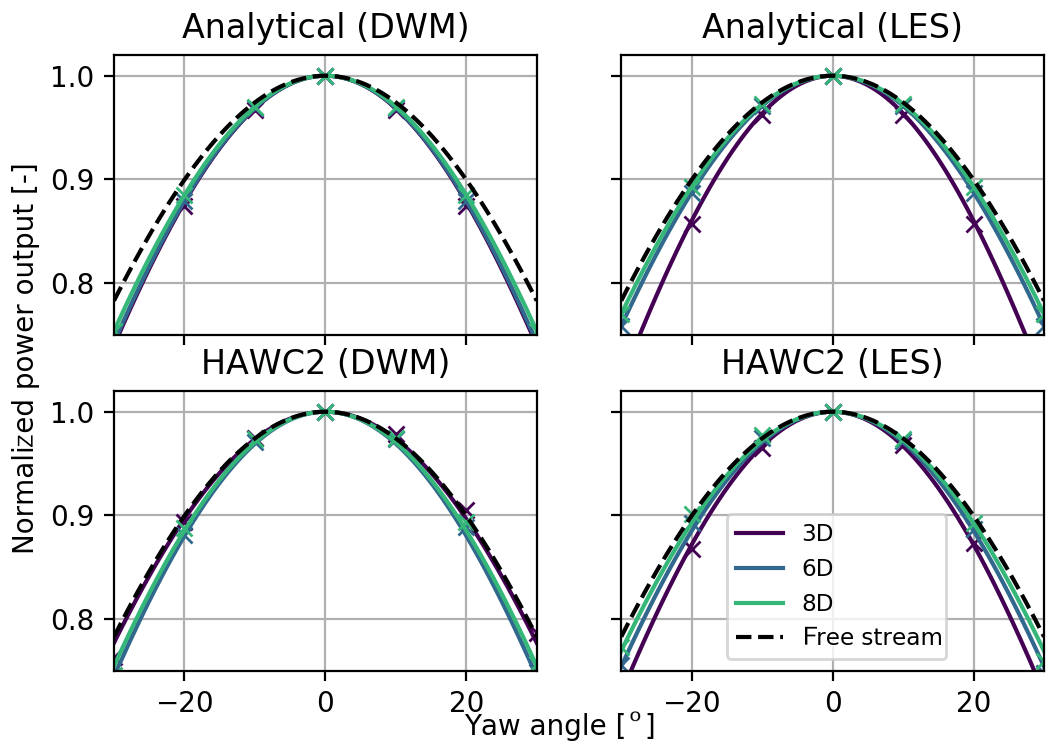
Figure 5Normalized power output as a function of yaw angle for different turbine spacings. Both calculation methods and wake generation tools are presented. The markers indicate the sample points used in the cosine fitting.
The analytical model shows good overall agreement with the aeroelastic simulations. For a turbine spacing between 5D and 8D, the relative difference between the analytical estimation of α and its respective aeroelastic simulation result is up to 2.7 %. For the far-wake region at distances larger than 8D, the analytical model and simulations show a lower relative difference in α of 0.4 %. The agreement between aeroelastic simulations and the analytical model is weaker in the near-wake scenarios; however, such low turbine spacings are rare in practice. Nevertheless, the general trend of an increased power–yaw loss exponent is still captured in this region for all four methods.
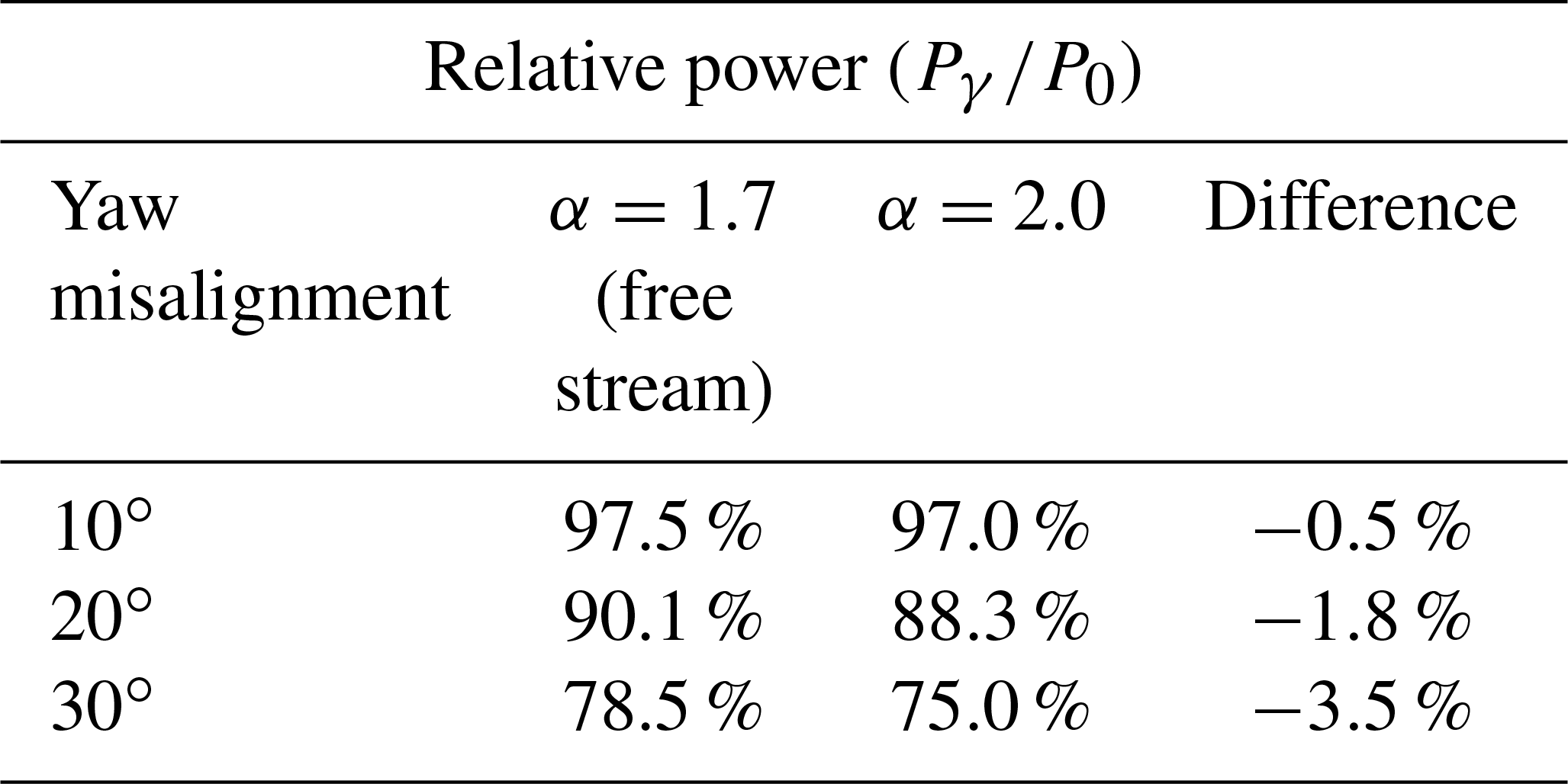
The maximum value of α at approximately 3D to 4D is due to the strong positive curvature of U(r) at small turbine spacings. As the wake recovers further downstream, this positive slope diminishes, and so α slowly converges to its free-stream value. The turbine spacing at which α peaks is closely related to the breakdown point, where the wake transitions from near wake to far wake (Sørensen et al., 2015). In terms of U(r), this point approximately corresponds to the downstream distance at which there is no longer a negative slope. The location of the α peak is dependant on the inflow conditions. In particular, a higher turbulence intensity will cause α to reach a maximum value at a lower turbine spacing due to a faster breakdown of the wake. An example of deviations in the power estimation that result from using a constant α compared to using the new adapted α is given in a wind farm layout consisting of two turbines with a spacing of 6D. Table 1 compares the normalized power output of the downstream turbine using α=2.0 based on the results shown in Fig. 6, and , which corresponds to the free-stream value shown previously. It can be seen that applying the free-stream value of α causes an overestimation of the power output when a downstream turbine is yawed, which increases with increasing yaw misalignment. Using typical values of yaw misalignment during wake steering (McKay et al., 2013), it is possible to experience a 3.5 % overestimation of the power output for a single turbine at 30∘ yaw misalignment. Hence, this effect can significantly change the outcome of full wind farm layout optimizations when including the wind direction uncertainty and particularly when attempting to develop wind farm control including intentionally yaw-misaligned turbines in the interior of wind farms.

Figure 6Power–yaw loss exponent as a function of turbine spacing for the four power calculation methods presented in this investigation.
Table 1Relative power output due to yaw misalignment for a downstream turbine located 6D downstream for α=2.0 and α=α0.
The estimation of α shows discrepancies in the near-wake region depending on the choice of wake generation method (LES or DWM). There are a number of potential sources for this discrepancy. Firstly, the two wake models, although having equal ambient conditions, present slight differences in the rate of mixing due to model differences. For this reason, the breakdown location of the LES wake appears at a shorter downstream distance than the DWM wake, which explains the α peak occurring at a smaller turbine spacing. Secondly, the LES wake is subject to effects not present in the DWM wake, causing differences in the azimuthal and time averaging. These factors include tip vortices, wake rotation, and ground effects.
Although the analytical model presented does not consider some physical effects, such as tip losses or rotor induction, the method shows close agreement with aeroelastic simulations in estimating the power–yaw loss exponent. The results are further reinforced by being able to capture the behavior of α for both medium- and high-fidelity wake profiles. This provides a correction for which power output can be adjusted for better estimations. It should be noted that the effects of rotor induction on the wake inflow, as well as both DWM- and LES-generated wakes, are not considered in the analytical model, HAWC2.
The investigation is limited to full-wake situations; however, by using the azimuthal-time averaging method described in Eq. (12), it is possible to extend the formulation in future work for asymmetric wakes, partial wakes, and curled wakes caused by turbine yaw misalignment.
This paper establishes the link between wake effects and the power sensitivity to yaw misalignment in a wind turbine, quantified by the power–yaw loss exponent, α. A clear trend is found in α through the analysis of HAWC2 aeroelastic simulations using both DWM- and LES-generated wake flow fields. Namely, α is largest for turbines operating in the near-wake region, and α converges to its free-stream value as turbine spacing increases. These trends are correctly captured by the analytical model for α presented in this paper. The theoretical formulation correctly anticipates the peak value of α, where the wake breaks down, and also converges to the free-stream conditions for large turbine spacing distances. The model shows how neglecting the influence of the wake on α can result in power production overestimation up to 3.5 % for a yaw misalignment of 30∘.
The simplified model presented in this paper provides a quick and reliable method to calculate α, which can be used for the optimization of wind farm layouts while including the uncertainty in the yaw misalignment of wind turbines operating in wake.
Lemna A1. The expected value, 𝔼[.], of a function, U(rm), is
where is the cumulative density function of rm.
Proof. The expected value of the random variable, U, is defined as
where fU(U) is the probability density function of U. Given that U is a function of radial position, U(rm), by the law of the unconscious statistician, Eq. (A2) can be written as
The range of rm is (rRcos γ, rR) as determined from the transformation in Eq. (2), hence the change in the integration limits. Integrating by parts gives
Lemna A2. Let Ψ∈[0, π] be a uniformly distributed random variable with the cumulative density function,
Let rm be a random variable defined as rm=g(Ψ), where
where , , π]. The cumulative distribution function, , of rm is
Proof. The cumulative distribution function of the random variable rm is given by
The steps to isolate Ψ yield the following:
From Eq. (A6),
Using the identity yields
Finally, from Eq. (A7), the range of rm is [rRcos (γ), rR], yielding the final expression:
The LES data that support the findings of this study are openly available in “LES of wake flow behind 2.3 MW wind turbine” at https://doi.org/10.11583/DTU.12005421.v1 (Andersen, 2020).
JL developed the theoretical formalism, performed the analytic calculations, and processed the aeroelastic simulation results. AMU performed the aeroelastic simulations using HAWC2. SJA generated the LES wake profiles. All authors contributed to the conceptualization, investigation, and reporting of the research presented in this paper.
The authors declare that they have no conflict of interest.
This paper was edited by Sandrine Aubrun and reviewed by Wim Munters and one anonymous referee.
Aagaard Madsen, H., Sørensen, N., and Schreck, S.: Yaw aerodynamics analyzed with three codes in comparison with experiment, in: AIAA Paper 2003-519, American Institute of Aeronautics and Astronautics, Reno, Nevada, USA, 2003. a
Andersen, S. J.: LES of wake flow behind 2.3 MW wind turbine, DTU Data, https://doi.org/10.11583/DTU.12005421.v1, 2020. a
Annoni, J., Bay, C., Johnson, K., Dall'Anese, E., Quon, E., Kemper, T., and Fleming, P.: Wind direction estimation using SCADA data with consensus-based optimization, Wind Energ. Sci., 4, 355–368, https://doi.org/10.5194/wes-4-355-2019, 2019. a
Archer, C. L. and Vasel-Be-Hagh, A.: Wake steering via yaw control in multi-turbine wind farms: Recommendations based on large-eddy simulation, Sustain. Energ. Technol. Assess., 33, 34–43, https://doi.org/10.1016/j.seta.2019.03.002, 2019. a
Bartl, J., Mühle, F., and Sætran, L.: Wind tunnel study on power output and yaw moments for two yaw-controlled model wind turbines, Wind Energ. Sci., 3, 489–502, https://doi.org/10.5194/wes-3-489-2018, 2018. a
Bossanyi, E.: Combining induction control and wake steering for wind farm energy and fatigue loads optimisation, J. Phys.: Conf. Ser., 1037, 032011, https://doi.org/10.1088/1742-6596/1037/3/032011, 2018. a, b
Dahlberg, J. and Montgomerie, B.: Research program of the utgrunden demonstration offshore wind farm, final report part 2, wake effects and other loads, Swedish Defense Research Agency, Kista, Sweden, 2005. a
DTU Wind Energy: DWMpy, Version 0.1, available at: https://gitlab.windenergy.dtu.dk/OpenLAC/DWMpy, last access: 28 August, 2019. a
Fleming, P., Gebraad, P., van Wingerden, J.-W., Lee, S., Churchfield, M., Scholbrock, A., Michalakes, J., Johnson, K., and Moriarty, P.: SOWFA Super-Controller: A High-Fidelity Tool for Evaluating Wind Plant Control Approaches, Tech. rep., National Renewable Energy Lab. (NREL), Golden, CO, USA, 2013. a
Fleming, P., Annoni, J., Churchfield, M., Martinez-Tossas, L. A., Gruchalla, K., Lawson, M., and Moriarty, P.: A simulation study demonstrating the importance of large-scale trailing vortices in wake steering, Wind Energ. Sci., 3, 243–255, https://doi.org/10.5194/wes-3-243-2018, 2018. a
Fleming, P. A., Ning, A., Gebraad, P. M., and Dykes, K.: Wind plant system engineering through optimization of layout and yaw control, Wind Energy, 19, 329–344, 2016. a
Gebraad, P., Thomas, J. J., Ning, A., Fleming, P., and Dykes, K.: Maximization of the annual energy production of wind power plants by optimization of layout and yaw-based wake control, Wind Energy, 20, 97–107, 2017. a, b
Gebraad, P. M., Teeuwisse, F., Van Wingerden, J., Fleming, P. A., Ruben, S., Marden, J., and Pao, L.: Wind plant power optimization through yaw control using a parametric model for wake effects – a CFD simulation study, Wind Energy, 19, 95–114, 2016. a, b
Gebraad, P. M. O., Fleming, P. A., and van Wingerden, J. W.: Comparison of actuation methods for wake control in wind plants, in: 2015 American Control Conference (ACC), Chicago, IL, USA, 1695–1701, https://doi.org/10.1109/ACC.2015.7170977, 2015. a
Howland, M. F., Lele, S. K., and Dabiri, J. O.: Wind farm power optimization through wake steering, P. Natl. Acad. Sci. USA, 116, 14495–14500, 2019. a
Hulsman, P., Andersen, S. J., and Göçmen, T.: Optimizing Wind Farm Control through Wake Steering using Surrogate Models based on High Fidelity Simulations, Wind Energ. Sci. Discuss., https://doi.org/10.5194/wes-2019-46, in review, 2019. a
Jiménez,Á., Crespo, A., and Migoya, E.: Application of a LES technique to characterize the wake deflection of a wind turbine in yaw, Wind Energy, 13, 559–572, 2010. a
Keck, R.-E.: Validation of the standalone implementation of the dynamic wake meandering model for power production, Wind Energy, 18, 1579–1591, 2015. a, b
Knudsen, T., Bak, T., and Svenstrup, M.: Survey of wind farm control–power and fatigue optimization, Wind Energy, 18, 1333–1351, 2015. a
Kragh, K. A., Hansen, M. H., and Mikkelsen, T.: Precision and shortcomings of yaw error estimation using spinner-based light detection and ranging, Wind Energy, 16, 353–366, https://doi.org/10.1002/we.1492, 2013. a
Larsen, G. C., Madsen, H. A., Thomsen, K., and Larsen, T. J.: Wake meandering: a pragmatic approach, Wind Energy, 11, 377–395, 2008. a
Larsen, T. J. and Hansen, A. M.: How 2 HAWC2, the user's manual, version 12-7, available at: http://www.hawc2.dk/download/hawc2-manual (last access: 1 June 2019), 2007. a
Larsen, T. J., Madsen, H. A., Larsen, G. C., and Hansen, K. S.: Validation of the dynamic wake meander model for loads and power production in the Egmond aan Zee wind farm, Wind Energy, 16, 605–624, 2013. a
Madsen, H. A., Larsen, G. C., Larsen, T. J., Troldborg, N., and Mikkelsen, R.: Calibration and validation of the dynamic wake meandering model for implementation in an aeroelastic code, J. Solar Energ. Eng., 132, 041014, https://doi.org/10.1115/1.4002555, 2010. a
Madsen, H. A., Larsen, T. J., Pirrung, G. R., Li, A., and Zahle, F.: Implementation of the blade element momentum model on a polar grid and its aeroelastic load impact, Wind Energ. Sci., 5, 1–27, https://doi.org/10.5194/wes-5-1-2020, 2020. a
Mann, J.: The spatial structure of neutral atmospheric surface-layer turbulence, J. Fluid Mech., 273, 141–168, 1994. a
Mann, J.: Wind field simulation, Probabil. Eng. Mech., 13, 269–282, 1998. a
McKay, P., Carriveau, R., and Ting, D. S.-K.: Wake impacts on downstream wind turbine performance and yaw alignment, Wind Energy, 16, 221–234, https://doi.org/10.1002/we.544, 2013. a, b, c, d
Medici, D.: Experimental studies of wind turbine wakes: power optimisation and meandering, PhD thesis, KTH, Stockholm, Sweden, 2005. a
Michelsen, J. A.: Basis3D-a platform for development of multiblock PDE solvers, Tech. rep., Technical Report AFM 92-05, Technical University of Denmark, Denmark, 1992. a
Mikkelsen, T., Hansen, K. H., Angelou, N., Sjöholm, M., Harris, M., Hadley, P., Scullion, R., Ellis, G., and Vives, G.: Lidar wind speed measurements from a rotating spinner, in: Ewec 2010 Proceedings Online, available at: https://backend.orbit.dtu.dk/ws/portalfiles/portal/4553836/Mikkelsen_EWEC_2010.pdf (last access: 1 June 2019), 2010. a
Munters, W. and Meyers, J.: Dynamic strategies for yaw and induction control of wind farms based on large-eddy simulation and optimization, Energies, 11, 177 https://doi.org/10.3390/en11010177, 2018. a, b
Nygaard, N. G.: Systematic quantification of wake model uncertainty, in: EWEA Offshore Conference, Copenhagen, Denmark, 10–12 March, 2015. a
Øye, S.: FLEX4 simulation of wind turbine dynamics, in: Proceedings of the 28th IEA Meeting of Experts Concerning State of the Art of Aeroelastic Codes for Wind Turbine Calculations (Available through International Energy Agency), Lyngby, Denmark, 11–12 April, 1996. a
Peña, A., Schaldemose Hansen, K., Ott, S., and van der Laan, M. P.: On wake modeling, wind-farm gradients, and AEP predictions at the Anholt wind farm, Wind Energ. Sci., 3, 191–202, https://doi.org/10.5194/wes-3-191-2018, 2018. a
Réthoré, P.-E., Fuglsang, P., Larsen, G. C., Buhl, T., Larsen, T. J., and Madsen, H. A.: TOPFARM: Multi-fidelity optimization of wind farms, Wind Energy, 17, 1797–1816, 2014. a
Schepers, J.: EU project in German Dutch wind tunnel, Technical Report ECN-RX-01-006, in: Energy Research Center of the Netherlands, ECN, the Netherlands, 2001. a
Schlipf, D., Schlipf, D. J., and Kühn, M.: Nonlinear model predictive control of wind turbines using LIDAR, Wind Energy, 16, 1107–1129, https://doi.org/10.1002/we.1533, 2013. a
Soleimanzadeh, M., Wisniewski, R., and Kanev, S.: An optimization framework for load and power distribution in wind farms, J. Wind Eng. Indust. Aerodynam., 107–108, 256–262, https://doi.org/10.1016/j.jweia.2012.04.024, 2012. a
Sørensen, J. N. and Shen, W. Z.: Numerical modeling of wind turbine wakes, J. Fluids Eng., 124, 393–399, 2002. a
Sørensen, J. N., Mikkelsen, R. F., Henningson, D. S., Ivanell, S., Sarmast, S., and Andersen, S. J.: Simulation of wind turbine wakes using the actuator line technique, Philos. T. Roy. Soc. A, 373, 20140071, https://doi.org/10.1098/rsta.2014.0071, 2015. a, b
Sørensen, N. N.: General purpose flow solver applied to flow over hills, Risø National Laboratory, Risø, Denmark, 1995. a
Urbán, A. M., Liew, J., Dellwik, E., and Larsen, G. C.: The effect of wake position and yaw misalignment on power loss in wind turbines, J. Phys.: Conf. Ser., 1222, 012002, https://doi.org/10.1088/1742-6596/1222/1/012002, 2019. a, b, c
Usually the spectral Kolmogorov constant is denoted by α, but here it has been represented with ϕ to avoid confusion with the power–yaw loss exponent.