Digitalization of scanning lidar measurement campaign planning

By using multiple wind measurements when designing wind farms, it is possible to decrease the uncertainty of wind farm energy assessments since the extrapolation distance between measurements and wind turbine locations is reduced. A WindScanner system consisting of two synchronized scanning lidars potentially represents a cost-effective solution for multipoint measurements, especially in complex terrain. However, the system limitations and limitations imposed by the wind farm site are detrimental to the installation of scanning lidars and the number and location of the measurement points. To simplify the process of finding suitable measurement positions and associated installation locations for the WindScanner system, we have devised a campaign planning workflow. The workflow consists of four phases. In the first phase, based on a preliminary wind farm layout, we generate optimum measurement positions using a greedy algorithm and a measurement “representative radius”. In the second phase, we create several Geographical Information System (GIS) layers such as exclusion zones, line-of-sight (LOS) blockage and lidar range constraint maps. These GIS layers are then used in the third phase to find optimum positions of the WindScanner systems with respect to the measurement positions considering the WindScanner measurement uncertainty and logistical constraints. In the fourth phase, we optimize and generate a trajectory through the measurement positions by applying the traveling salesman problem (TSP) on these positions. The described workflow has been digitalized into a Python package named campaign-planning-tool, which gives users an effective way to design measurement campaigns with WindScanner systems. In this study, the Python package has been tested on three different sites characterized by different terrain complexity and wind farm dimensions and layouts. With minimal effort, the Python package can optimize measurement positions and suggest possible lidar installation locations for carrying out resource assessment campaigns.

1 Introduction

The development of a wind farm project begins with an assessment of the wind resources and the energy yield for the planned wind farm. Best practices recommend estimating wind resources based on local wind measurements (MEASNET, 2016). Measurement campaigns designed for wind resource assessment have historically relied on anemometers and wind vanes mounted on tall meteorological masts (also called met masts) to measure a wind climate similar to the wind climate the wind turbines will experience during their lifetime. The local measurements are used to produce the observed wind climate of the site. To account for the seasonal and interannual variations of the wind, the observed wind climate is long-term corrected using long-term reference data from a nearby meteorological station, reanalysis data or mesoscale models (Carta et al., 2013). The long-term-corrected wind climate is then extrapolated vertically and horizontally, typically using a flow model such as WAsP (Mortensen et al., 2014) to estimate the wind resource at hub height for every wind turbine location.

The single mast approach is affordable but can cause large uncertainties. Specifically, in complex terrain (mountainous and forested areas), the spatial extrapolation becomes challenging as the topography can significantly influence the flow. The ideal scenario would be to measure the local wind climate at every planned wind turbine position. However, erecting as many masts as wind turbines would be extremely costly and in some areas impossible.

Many large wind farm projects in complex terrain are developed using multiple masts. Combining one fixed mast and one or several roaming profiling lidars moved to different positions during the campaign is another option. The advantage of roaming vertical profiling lidars lies in their ability to provide affordable high-altitude measurements, ease of deployment and no need for building permits in comparison to the masts, while data availability and inaccuracy in complex terrain (Bingöl et al., 2009) are some of their disadvantages. However, any roaming setup brings a trade-off between the number of measurement positions and the measurement duration at each location since short measurements (e.g., of 3 months) can lead to erroneous wind climate (Langreder and Mercan, 2016).

A potential solution for multipoint measurements for wind resource assessment lies in the application of scanning lidars (Krishnamurthy et al., 2013). With a measurement range of several kilometers and a beam that can be oriented freely in any direction (Vasiljević et al., 2016), many measurement positions can be reached without moving the hardware. Especially dual-Doppler setups (i.e., two scanning lidars) can provide accurate retrieval of horizontal wind speed and wind direction (i.e., two-dimensional, 2-D, wind vector) at many possible positions (Vasiljević et al., 2017). While scanning lidars provide a broad range of benefits, there are also clear challenges when designing multilidar measurement campaigns.

The biggest challenge when designing a multilidar measurement campaign is deciding where to measure and how to position scanning lidars to acquire accurate measurements. As mentioned before, we would like to measure at every future wind turbine location. Realistically, in the case of large wind farms (many wind turbines), this is not feasible. As the laser beams need to traverse each turbine location, there would not be enough measurement samples per location to do a proper statistical analysis of the wind resources. A good rule of thumb is to have at least 10 samples for each measurement point per 10 min period. Therefore, we would need an approach to minimize the number of measurement points such that we satisfy spatial and temporal coverage of the wind farm resources (i.e., enough samples and a good distribution of measurements across the farm site).

Afterward, constraints that arise from scanning lidars, atmosphere and site characteristics dictate the positioning of lidars. Indeed, the laser beam of scanning lidars can be steered freely, but, on the other hand, it can be blocked in some directions by the terrain, vegetation or other obstacles. This impacts the lidar positioning since we need an unobstructed passage of the laser beams towards measurement points, i.e., clear line of sight (LOS). On the other hand, the lidar characteristics (e.g., laser wavelength and output power) in combination with the atmosphere characteristics (e.g., aerosol extinction, backscatter coefficient and atmospheric attenuation) impact the lidar range. Furthermore, retrieving the 2-D wind vector requires a limited beam elevation angle (e.g., smaller than 5^∘ as suggested by Vasiljević et al., 2017) to avoid contamination of horizontal wind components with the vertical component. Finally, the intersecting angle of the laser beams at the measurement points should be large enough (e.g., greater than 30^∘ as suggested by Vasiljević and Courtney, 2017) to minimize the lidar measurement uncertainty (Davies-Jones, 1979; Stawiarski et al., 2013).

Once the lidar positions are set and measurement points determined, generating an optimized trajectory is essential to reduce the motion time from one measurement point to another, and thus boost the sampling rate per measurement point. Overall, at the same time, a campaign designer has to handle several constraints to find the best measurement locations and accordingly generate the best possible measurement campaign layout, or they can decide that a measurement campaign with scanning lidars is not practical.

In this paper, we describe a workflow which tackles the above-described challenges involved in the planning of scanning lidar campaigns together with an approach of the workflow digitalization. The workflow is based on the application of the methodology for multilidar experiments on wind resource assessment campaigns (Vasiljević et al., 2017), which was previously used in planning of measurement campaigns conveyed in the New European Wind Atlas (NEWA) project (Mann et al., 2017), such as Perdigao-2015 (Vasiljević et al., 2017) and Perdigao-2017 (Fernando et al., 2019). The workflow addresses “experiment layout design” and “scanning modes design” steps of the abovementioned methodology (see steps 4 and 5 in Vasiljević et al., 2017).

The paper is organized as follows. Section 2 provides a detailed description of the four main phases of the workflow. Additionally, Sect. 2 provides a recipe for the workflow digitalization. In Sect. 3 we present results of applying the digitalized workflow for planning campaigns at three wind farm sites that are different in size, layout and complexity. Results and further development of the workflow are discussed in Sect. 4, and we provide our concluding remarks in Sect. 5.

2 Methodology

2.1 Overview

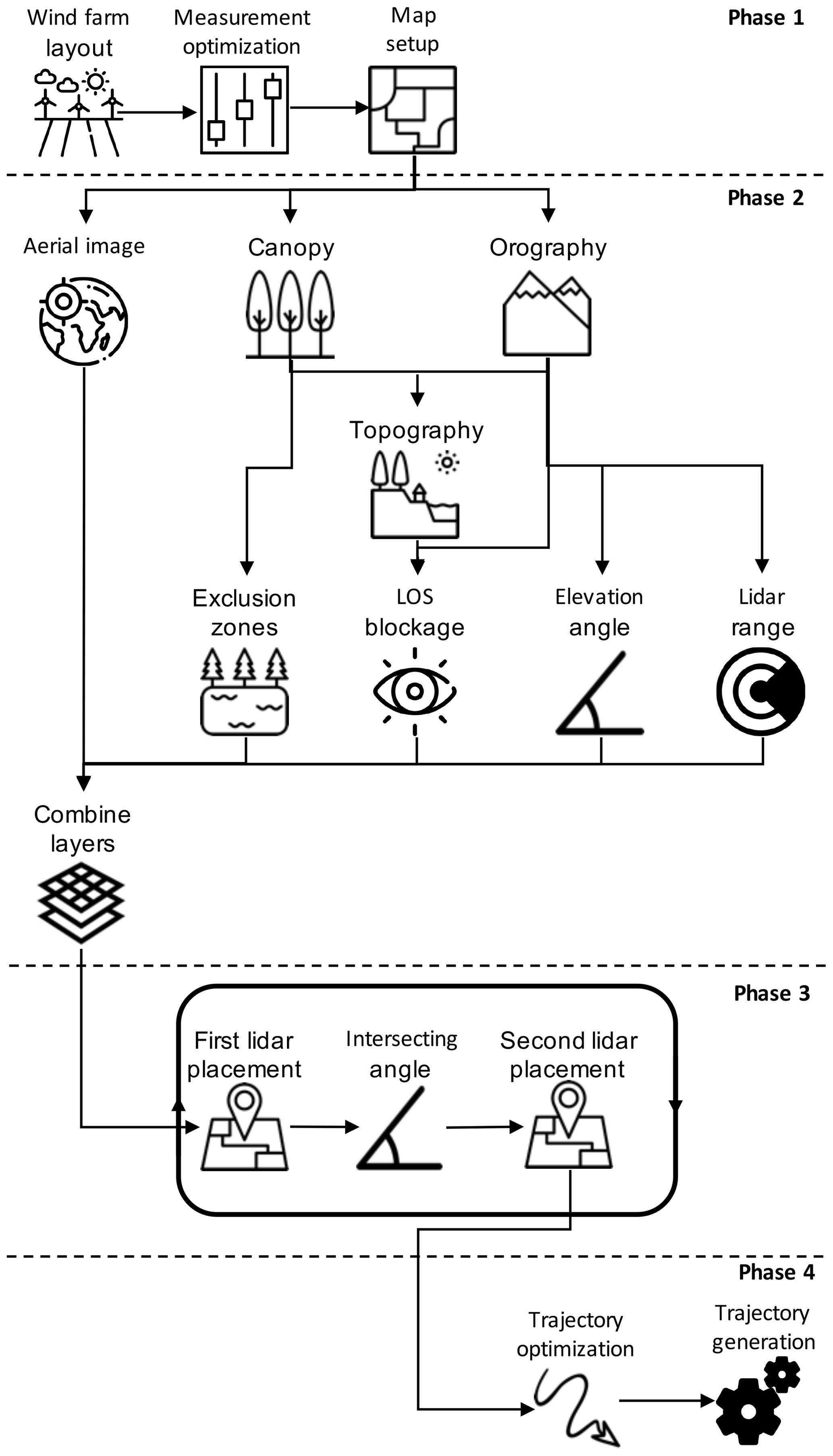
We assume that the location and the layout of the wind farm are known. This initial information is input to the campaign planning workflow, which consists of four sequential phases graphically represented in Fig. 1. First of all, if required the measurement positions are optimized based on the wind farm layout. Afterward, the measurement positions are used in combination with lidar and site constraints to generate the map that highlights the best lidar installation locations. In the next phase, the positions of the scanning lidars are determined by minimizing a dual-Doppler measurement uncertainty of horizontal wind speed while identifying existing road and power infrastructure. Finally, considering the measurement positions and positions of scanning lidars, the trajectory of the laser beams through all the reachable measurement points is optimized and afterward generated. In the sections that follow, each phase will be described in detail.

Figure 1 Campaign planning workflow (figure designed using © freepik.com icon database).

2.2 Phase 1 – measurement positions optimization

This first phase of the workflow tackles challenges of measurement point optimization. We assume that the wind farm site has been selected and that a preliminary resource assessment and wind farm layout have been made before the campaign planning.

For small wind farms (either a limited number of turbines and/or a limited spatial extent), we consider the wind turbine positions as the measurement positions. For larger wind farms, the number of measurement points needs to be reduced. However, the reduced set of measurement points should be adequately distributed over the wind farm site to avoid long wind resource extrapolation distances. The simplest approach is to group the wind turbine locations, which are close to each other in clusters and to assign a single measurement location per cluster. MEASNET (2016) suggests that measurements from a single location represent the wind climate over a certain area described by “representativeness radius” (R_r). R_r has different values for different terrain types. For example, in complex terrain, the radius should be smaller than 2 km as suggested by MEASNET (2016). By solving a disk-covering problem (e.g., Biniaz et al., 2017), in which we aim to find a minimum number of disks with a radius equal to R_r that cover all locations of wind turbines, we cluster the wind turbines and optimize the measurement locations. As stated in Ghasemalizadeh and Razzazi (2012), there are several ways to solve the disk-covering problem. One of them is a greedy approach that we adapted to suit our purpose.

In our case, the greedy algorithm implementation yields the set D of m unique disks with the radius R_r covering the set T of n wind turbine positions ($T=\mathit{\{}{T}_{\mathrm{1}},T_{\mathrm{2}},\mathrm{\dots },T_n\mathit{\}}$). We are solving the disk-covering problem in two dimensions (2-D) by omitting the height coordinate (i.e., z) of turbine positions. The greedy algorithm implementation can be described in the algorithmic sense with the following steps:

1. Initialize the set D (D=∅).

2. For any unique pair of wind turbine positions (there is $p=\frac{n\mathrm{!}}{\mathrm{2}(n-\mathrm{2})\mathrm{!}}$ unique pairs), calculate a midpoint M_i, which is considered a potential disk center, and add it to the set $M=\mathit{\{}{M}_{\mathrm{1}},M_{\mathrm{2}},\mathrm{\dots },M_p\mathit{\}}$.

3. Find the elements of the set T that are covered by each element of the set M and form an additional set S which will contain this information. To do this, calculate the distance between each element of the two sets:

   $$\begin{array}{}\text{(1)}& \begin{array}{rl}{d}_{i,j}& =\parallel M_i-T_j\parallel \\ & =\sqrt{{\left(x_{M_i}-x_{T_j}\right)}^{\mathrm{2}}+{\left(y_{M_i}-y_{T_j}\right)}^{\mathrm{2}}},\\ & i=\mathrm{1},\mathrm{\dots },p\wedge j=\mathrm{1},\mathrm{\dots },n,\end{array}\end{array}$$

   where x_m, y_m, x_t, and y_t are coordinates of disk centers and turbine positions; then compare d_i,j to R_r (the d_i,j ≤ R_r condition must be satisfied for a disk M_i to cover a point T_j). Through the comparisons, the set S is formed. The elements of S are actually sets themselves containing wind turbine positions covered by each disk from the set M. If, for example, a disk M_k covers turbine positions T₁, T₂ and T_n (i.e., d_k,1, d_k,2 and d_k,n are smaller or equal to R_r), the corresponding element of the set S, i.e., S_k, will contain these elements (i.e., $S_k=\mathit{\{}{T}_{\mathrm{1}},T_{\mathrm{2}}\mathrm{and}{T}_n\mathit{\}}$). Alternatively, if a disk M_k does not cover any turbine position, the corresponding element of the set S will be an empty set (i.e., S_k=∅).

4. Select a disk from the set M which covers the maximum number of points of the set T (this process is aided using the set S). Let this disk be M_i.

5. The disk M_i is added to D and removed from M:

   $$\begin{array}{}\text{(2)}& {\displaystyle }D=D\cup M_i,\text{(3)}& {\displaystyle }M=M\cap M_i,\text{(4)}& {\displaystyle }S=S\cap S_i.\end{array}$$

6. Points covered by M_i provided in S_i are removed from the set T and from any subset of the set S:

   $$\begin{array}{}\text{(5)}& {\displaystyle }T=T\cap S_i,\text{(6)}& {\displaystyle }\forall S_j\in S,S_j=S_j\cap S_i.\end{array}$$

7. Steps 1 to 6 are repeated until either the set T or S is empty :

   $$\begin{array}{}\text{(7)}& T=\mathrm{\varnothing }\vee S=\mathrm{\varnothing }.\end{array}$$

8. If T is not an empty set after Step 7, then the remaining elements are added to the set D:

   $$\begin{array}{}\text{(8)}& D=D\cup T.\end{array}$$

At the end of this process, elements of the set D, i.e., measurement points, contain only x and y coordinates. Using the digital elevation model (DEM) from the Shuttle Radar Topography Mission (SRTM; Farr et al., 2007) we can introduce the height information to the elements of the set D. It is important to additionally add the hub height of future wind turbines to this height information. As the last step of the first phase, we generate a mesh of equally spaced points over the site with the measurement point in the mesh center (see Fig. 2). Let us denote the mesh as G and treat it as a set of elements G_i,j ($G_{i,j}=\mathit{\{}{x}_i,y_j\mathit{\}}$, where $i=j=\mathrm{1},\mathrm{\dots },l$). The mesh resolution should be equal to the land cover and terrain data resolution which will be used in the second phase (typically $\mid x_{\mathrm{2}}-x_{\mathrm{1}}\mid =\mid y_{\mathrm{2}}-y_{\mathrm{1}}\mid =\mathrm{100}$ m). This avoids any interpolation of the land cover or topography datasets to our mesh.

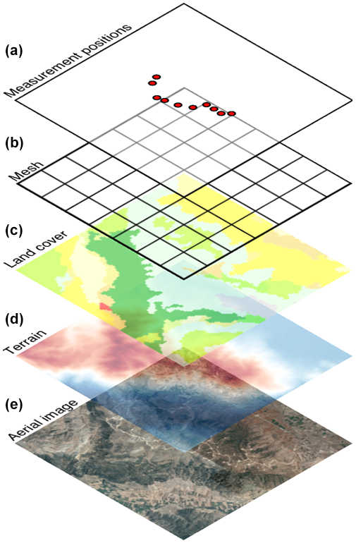
Figure 2 A stack of data used to generate the GIS layer for lidar placement: (a) measurement positions generated by solving the disk-covering problem; (b) mesh covering wind farm site; (c) land cover data sourced from CORINE Land Cover database; (d) terrain data sourced from SRTM DEM database and (e) aerial image sourced from the © Google Maps server.

2.3 Phase 2 – highlighting best lidar installation locations

In this phase, we will create a Geographical Information System (GIS) layer which includes site and lidar constraints while highlighting the best lidar installation locations considering the previously determined measurement points. We will denote this GIS layer as the combined layer and treat it as a set C_l containing elements $C_{\mathrm{l},i,j}$. To create this layer, first we acquire land cover data, orthography data and the aerial image corresponding to the extent of the previously generated mesh (Fig. 2). For land cover data, we can use the CORINE Land Cover dataset. In the case of the orography, the previously mentioned SRTM DEM datasets serve this purpose, and for the aerial image we can use the Google Maps server. All three data sources are publicly available. The acquired stack of data will be a base material for the combined layer creation.

At present we consider five types of constraints which are detrimental for a lidar installation: zones where a lidar cannot be installed (e.g., lakes, forests, etc.); topographical features that can block the beam; keeping the lidar elevation angle below a certain threshold to avoid measurement contamination with the vertical component of the wind; the maximum lidar range; practical matters such as access roads. To create the combined layer which contains all the above-listed constraints, first we will generate GIS layers for each constraint and afterward merge them. These individual GIS layers are (1) exclusion zones layer, (2) LOS blockage layer, (3) elevation angle layer, (4) lidar range layer and (5) logistical layer.

To create the exclusion zone layer we will use the land cover data and according to the land cover type (e.g., water surface, forest, etc.) classify areas of the site as suitable or not for a lidar installation. The land cover data can be treated as a set Lc of equally spaced elements Lc_i,j containing integer values which represent the so-called grid_code that indicates the land cover type (e.g., water bodies have grid_code code from 40 to 44). A look-up table for grid_code comes together with the land cover data when downloaded from the CORINE Land Cover web site (https://land.copernicus.eu/pan-european/corine-land-cover/, last access: 9 January 2020). To generate the exclusion zone layer we make a copy of the mesh (an empty mesh), walk through the mesh (going from one mesh point to another), fetch the corresponding information on land cover type from the land cover dataset, check the type and assign a value of 1 or 0 to the mesh point if the land cover type allows lidar installation or not (e.g., $G_{i,j}=\mathit{\{}{x}_i,y_i,\mathrm{1}\mathit{\}}$ if grid_code code is equal to 12, i.e., “arable land”). An example of a fictive exclusion zone layer is shown in Fig. 3.

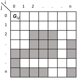
Figure 3 Fictive exclusion zone layer represented as an array: G_i,j denotes one mesh point, white and gray squares indicate bad ($G_{i,j}=\mathrm{0}$) and good ($G_{i,j}=\mathrm{1}$) locations for a lidar installation, respectively, and i corresponds to x coordinate or easting and j corresponds to y coordinate or northing.

To generate the LOS blockage layer we need to create a dataset that contains the summed height of terrain and canopy. To do this we will add 20 m at each location in the DEM dataset where the CORINE Land Cover dataset contains code which corresponds to the forest (grid_code code equal to 23, 24 and 25). This value is a conservative guess. Afterwards, we make a copy of the mesh, walk through the mesh, fetch the corresponding elevation from the DEM dataset, perform a viewshed analysis (Izraelevitz, 2003) from the selected mesh point to each measurement point that returns which measurement points are visible and assign the visible measurement points to the mesh point (e.g., if measurement points D₁, D₂ and D_n are visible from G_i,j, then $G_{i,j}=\mathit{\{}{x}_i,y_i,D_{\mathrm{1}},D_{\mathrm{2}},D_n\mathit{\}}$). In the viewshed analysis for the selected mesh point, we are only taking the corresponding height from the DEM dataset (since we consider that lidar will be installed on the ground), while for the points in between the mesh and measurement points we are considering the summed height dataset. The result of this process is the LOS blockage layer, whose mesh points contain a set of measurement points to which there is an unobstructed LOS.

Our focus is to design a dual-Doppler measurement campaign to retrieve the horizontal wind speed. Accordingly, a low elevation beam angle is required to avoid contamination of the LOS speed measurement with the vertical component of the wind vector. We create the elevation angle layer to serve this purpose. This layer is created through the following steps: we make a copy of the mesh, walk through each mesh point, fetch the height information from the DEM dataset, calculate the elevation angle from the mesh point to each measurement point, compare the calculated angle to a threshold value (e.g., a maximum of 5^∘ as suggested by Vasiljević et al., 2017) and assign measurement points to the mesh point for which the elevation angle is below the threshold value.

In the lidar range layer, mesh points contain measurement points that are within reach of the lidar taking into account the expected range of the lidar for the given site. It is worth noting that the expected range is not the maximum range given in the product data sheet. The layer is created similarly to the previous one.

To create the combined layer, we will treat the four previously derived layers as sets E_z (exclusion zone layer), L_b (LOS blockage layer), E_a (elevation angle layer) and L_r (lidar range layer). Since each set is made using the same mesh, each set contains the same number of elements. The combined layer, treated as a set C_l containing elements $C_{\mathrm{l},i,j}$, is derived as follows:

$$\begin{array}{}\text{(9)}& {\displaystyle }{C}_{\mathrm{l}}=\mathit{\{}{C}_{\mathrm{l},\mathrm{1},\mathrm{1}},C_{\mathrm{l},\mathrm{1},\mathrm{2}},\mathrm{\dots },C_{\mathrm{l},l,l}\mathit{\}};\text{(10)}& {\displaystyle }{C}_{\mathrm{l},i,j}=\left\{\begin{array}{ll}\mathit{\{}{x}_i,y_j,\mathit{\{}\mathit{\left\}}\mathit{\right\}}& \text{if }{E}_{\mathrm{z},i,j}=\mathit{\{}{x}_i,y_i,\mathrm{0}\mathit{\}},\\ L_{\mathrm{b},i,j}\cap E_{\mathrm{a},i,j}\cap L_{\mathrm{r},i,j}& \text{if }{E}_{\mathrm{z},i,j}=\mathit{\{}{x}_i,y_i,\mathrm{1}\mathit{\}}.\end{array}\right.\end{array}$$

Therefore, the mesh points of the combined layer will contain which and how many measurement points are reachable considering the first four above-described constraints.

Finally, the acquired aerial image of the site (the logistical layer) is kept separately and will serve the important purpose of identifying existing road and power infrastructure.

2.4 Phase 3 – placement of the lidars

The combined layer together with the underlying aerial image highlights the “best” locations for the placement of individual lidars considering all the above-described constraints. However, designing the campaign for a dual-Doppler system, where beams from two lidars need to synchronously cross every measurement position, adds one more constraint, which is the limitation on the beams intersection angle. The measurement uncertainty of a dual-Doppler system increases when the intersecting angle between the laser beam becomes small (see Vasiljević and Courtney, 2017). Therefore the position of the second lidar is very much determined by the position of the first lidar. Considering that we have chosen the first lidar location using the combined layer and the logistical layer, now we need to calculate an additional layer to which we will refer as the intersecting angle layer. This layer is created as following: we make a copy of the mesh, walk through each mesh point considering each mesh point as a second lidar position, calculate intersecting angles between the two laser beams at each measurement point and add those measurement points to the mesh point for which the intersecting angle is bigger than a specific value (e.g., at least 30^∘ as suggested by Davies-Jones, 1979; Vasiljević and Courtney, 2017). Let us treat this GIS layer as a set I_a with elements $I_{\mathrm{a},i,j}$. To highlight the best locations for the second lidar installation, the intersecting angle layer should be intersected with the combined layer, i.e.,

$$\begin{array}{}\text{(11)}& S_{\mathrm{l}}=C_{\mathrm{l}}\cap I_{\mathrm{a},i,j},\end{array}$$

where S_l is a set corresponding to the newly created GIS layer for the second lidar placement. The process of selecting a position for the first lidar, followed by the generation of the layer for locating the second lidar and selection of the second lidar position, should be performed several times to generate several potential experiment designs, since only during a field visit will it be possible to determine the most likely design for the measurement campaign. Once the second lidar position is determined, we derive a set of reachable measurement points D_r by both lidars, which is a subset of the set D (D_r∈D).

2.5 Phase 4 – trajectory optimization and generation

The fourth phase consists of the optimization of the path through the measurement points (to boost the sampling rate) and the generation of the synchronized trajectories for two scanning lidars.

One way to optimize the path through the measurement points is to adapt the traveling salesman problem (TSP). In the regular TSP, the goal is to find the shortest path through a set of n cities that a traveling salesman needs to visit. There are multiple approaches to solve the TSP (Reinelt, 1994). One of the simplest implementations for solving the TSP is nearest neighbor heuristics (NNH). As stated in (Reinelt, 1994):

This heuristic for constructing a traveling salesman tour is near at hand. The salesman starts in some city and then visits the city nearest to the starting city. From there he visits the nearest city that was not visited so far, etc., until all cities are visited, and the salesman returns to the start.

In our case, we have a single set of measurement points D_c which need to be simultaneously visited by the two laser beams. Since typically two scanning lidars will not be symmetrically positioned with respect to the measurement points we will have two different sets of steering angles D_s1 and D_s2 corresponding to the first and second lidar, respectively, that enable “visiting” the measurement points with the laser beams. Therefore, we cannot directly apply the above-described heuristics. The TSP NNH solution needs to be adapted.

Let us consider that the set D_c is defined as

$$\begin{array}{}\text{(12)}& D_c=\mathit{\{}{D}_{c,\mathrm{1}},D_{c,\mathrm{2}},\mathrm{\dots },D_{c,n}\mathit{\}},D_{c,i}=\mathit{\{}{x}_i,y_i,z_i\mathit{\}},\end{array}$$

while D_s1 and D_s2 are defined as

$$\begin{array}{}\text{(13)}& {\displaystyle }{D}_{\mathrm{s}\mathrm{1}}=\mathit{\{}{D}_{\mathrm{s}\mathrm{1},\mathrm{1}},D_{\mathrm{s}\mathrm{1},\mathrm{2}},\mathrm{\dots },D_{\mathrm{s}\mathrm{1},\mathrm{n}}\mathit{\}},D_{\mathrm{s}\mathrm{1},\mathrm{i}}=\mathit{\{}{\mathit{\theta }}_{\mathrm{1},i},{\mathit{\phi }}_{\mathrm{1},i}\mathit{\}},\text{(14)}& {\displaystyle }{D}_{\mathrm{s}\mathrm{2}}=\mathit{\{}{D}_{\mathrm{s}\mathrm{2},\mathrm{1}},D_{\mathrm{s}\mathrm{2},\mathrm{2}},\mathrm{\dots },D_{\mathrm{s}\mathrm{2},\mathrm{n}}\mathit{\}},D_{\mathrm{s}\mathrm{2},\mathrm{i}}=\mathit{\{}{\mathit{\theta }}_{\mathrm{2},i},{\mathit{\phi }}_{\mathrm{2},i}\mathit{\}},\end{array}$$

where θ and φ are azimuth and elevation angles, respectively. Additionally, we will make a set I which will contain indexes of the sets' elements:

$$\begin{array}{}\text{(15)}& I=\mathit{\{}\mathrm{1},\mathrm{2},\mathrm{\dots },j,\mathrm{\dots },n\mathit{\}}.\end{array}$$

The adapted TSP NNH solution for dual-Doppler trajectory can be described in the algorithmic sense with the following steps:

1. Initialize empty sets T_l1 and T_l2 ($T_{\mathrm{l}\mathrm{1}}=T_{\mathrm{l}\mathrm{2}}=\mathrm{\varnothing }$), which will contain ordered elements of the optimized trajectory (i.e., the trajectory points).

2. Select an arbitrary index j from the set I.

3. Set an element l to j (l=j).

4. Select elements D_s1,l and D_s2,l.

5. Add the elements D_s1,l and D_s2,l to the set T_l1 and T_l2, respectively, and remove index j and elements D_s1,l and D_s2,l from the set I, D_s1 and D_s2, respectively:

   $$\begin{array}{}\text{(16)}& {\displaystyle }{T}_{\mathrm{l}\mathrm{1}}=T_{\mathrm{l}\mathrm{1}}\cup D_{\mathrm{s}\mathrm{1},\mathrm{l}},\text{(17)}& {\displaystyle }{T}_{\mathrm{l}\mathrm{2}}=T_{\mathrm{l}\mathrm{2}}\cup D_{\mathrm{s}\mathrm{1},\mathrm{2}},\text{(18)}& {\displaystyle }I=I\cap j,\text{(19)}& {\displaystyle }{D}_{\mathrm{s}\mathrm{1}}=D_{\mathrm{s}\mathrm{1}}\cap D_{\mathrm{s}\mathrm{1},\mathrm{l}},\text{(20)}& {\displaystyle }{D}_{\mathrm{s}\mathrm{2}}=D_{\mathrm{s}\mathrm{2}}\cap D_{\mathrm{s}\mathrm{2},\mathrm{l}}.\end{array}$$

6. Calculate sets Δα₁ and Δα₂, which contain elements Δα_1,il and Δα_2,il (i takes values from the set I), defined as

   $$\begin{array}{}\text{(21)}& {\displaystyle }\begin{array}{rl}\mathrm{\Delta }{\mathit{\alpha }}_{\mathrm{1},il}& =\mathit{\{}\mid {\mathit{\theta }}_{\mathrm{1},i}-{\mathit{\theta }}_{\mathrm{1},l}\mid ,\mid {\mathit{\phi }}_{\mathrm{1},i}-{\mathit{\phi }}_{\mathrm{1},l}\mid \mathit{\}}\\ & i=\mathrm{1},\mathrm{2},\mathrm{\dots },n;\end{array}\text{(22)}& {\displaystyle }\begin{array}{rl}\mathrm{\Delta }{\mathit{\alpha }}_{\mathrm{2},il}& =\mathit{\{}\mid {\mathit{\theta }}_{\mathrm{2},i}-{\mathit{\theta }}_{\mathrm{2},l}\mid ,\mid {\mathit{\phi }}_{\mathrm{2},i}-{\mathit{\phi }}_{\mathrm{2},l}\mid \mathit{\}}\\ & i=\mathrm{1},\mathrm{2},\mathrm{\dots },n\end{array}\end{array}$$

   that describe relative angular moves for the two lidars from the measurement point described by the last element of the sets T_l1 and T_l2 (i.e., D_s1,l and D_s2,l, respectively) to all remaining measurement points described by elements of D_s1 and D_s2.

7. Form a set B containing maximum concurring elements of the sets Δα₁ and Δα₂:

   $$\begin{array}{}\text{(23)}& \begin{array}{rl}B& =\mathit{\{}max(\mathrm{\Delta }{\mathit{\alpha }}_{\mathrm{1},\mathrm{1}l},\mathrm{\Delta }{\mathit{\alpha }}_{\mathrm{2},\mathrm{1}l}),max(\mathrm{\Delta }{\mathit{\alpha }}_{\mathrm{1},\mathrm{2}l},\mathrm{\Delta }{\mathit{\alpha }}_{\mathrm{2},\mathrm{2}l}),\\ & \mathrm{\dots },max(\mathrm{\Delta }{\mathit{\alpha }}_{\mathrm{1},\mathrm{1}n},\mathrm{\Delta }{\mathit{\alpha }}_{\mathrm{2},\mathrm{1}n})\mathit{\}}.\end{array}\end{array}$$

8. Find index j of an element of the set B which has lowest value.

9. Repeat steps 3 to 8 until the sets D_s1 and D_s2 are empty ($D_{\mathrm{s}\mathrm{1}}=D_{\mathrm{s}\mathrm{2}}=\mathrm{\varnothing }$).

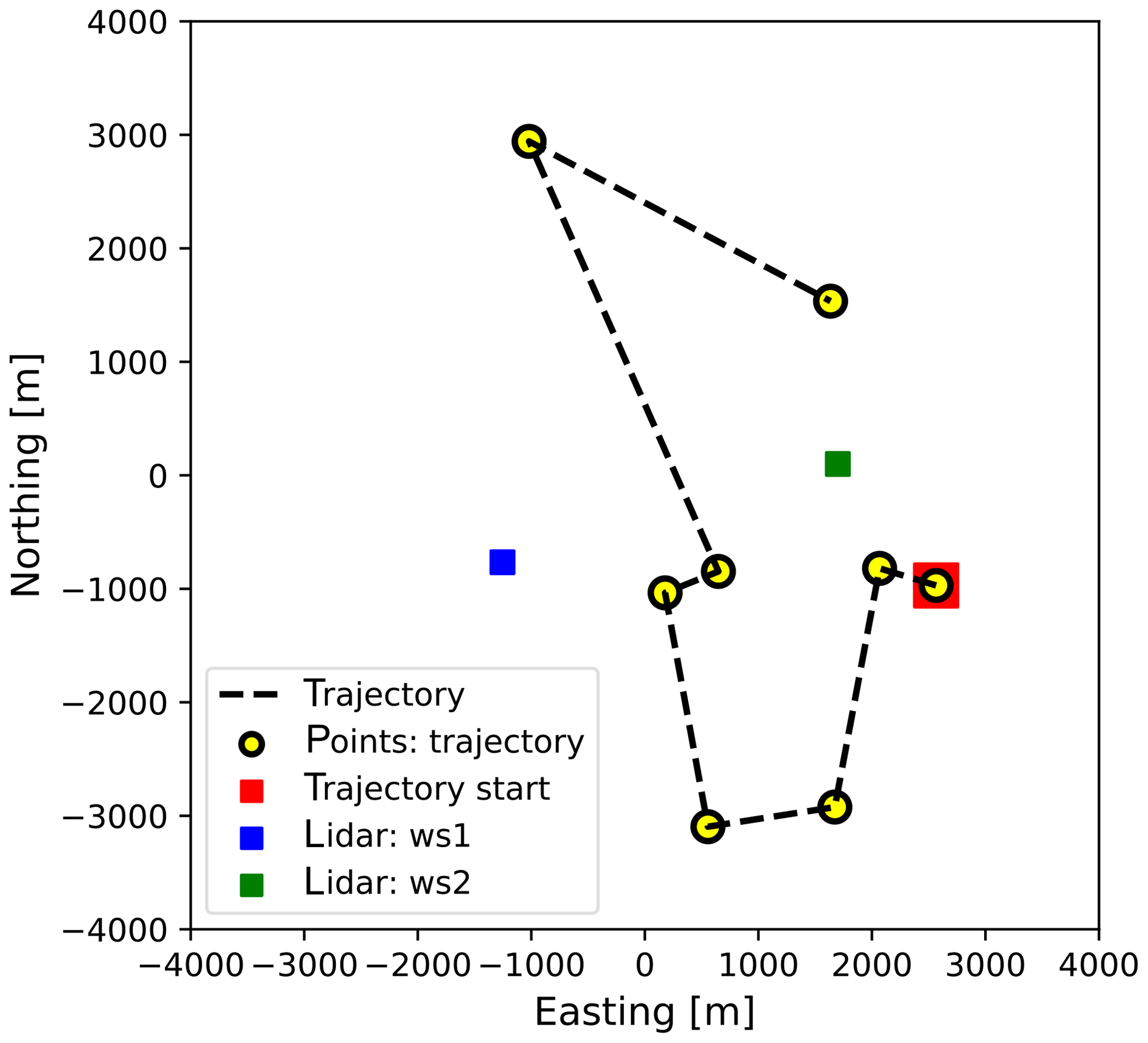
The main modification of a standard TSP NNH solution is the addition of Step 7, which ensures that the trajectory will be optimal for both lidars instead of only one. The difference between the standard and adapted TSP NNH solution can be seen from an example shown in Fig. 4.

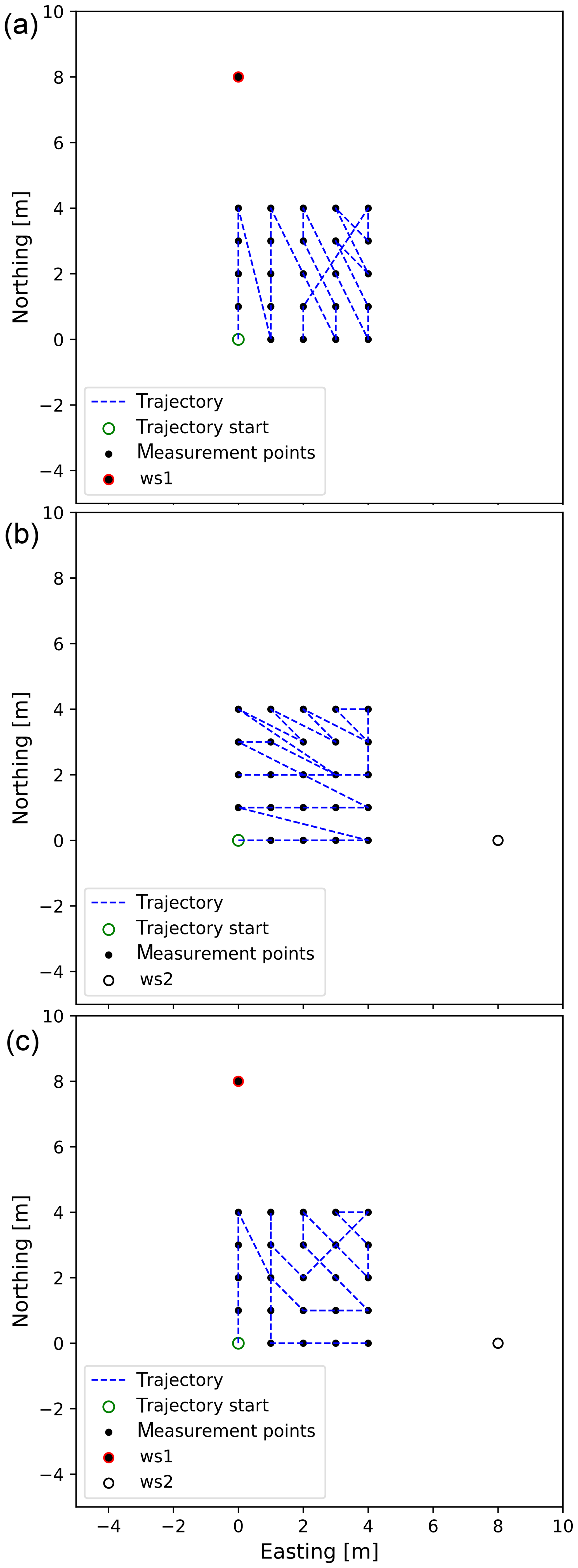
Figure 4 TSP NNH: (a) standard TSP NNH for lidar denoted ws1; (b) standard TSP NNH for lidar denoted ws2; (c) adapted TSP NNH for two lidars denoted ws1 and ws2.

To get the lidars to follow the optimized trajectory, we need to describe the motion of the scanners as a function of time. In other words, we need to add the time component of the trajectory to the spatial description we yielded in the previous steps. When calculating the timing for the trajectory, we assume that the lidars will stop at each measurement point and sample wind speed before they continue to the next measurement point. Therefore, we expect that lidars will perform so-called step-stare trajectories. There are several reasons for selecting step-stare trajectories instead of continuously scanning the flow through the trajectory described by the measurement points. Step-stare trajectories are simpler for the implementation and synchronization of multiple lidars; also, the step-stare data processing is less complex when compared to the continuously scanning trajectories.

The timing for the step-stare scans can be calculated using a simple solution for the kinematics elevator problem (KEP) (e.g., Al-Sharif, 2014) considering an infinite jerk:

$$\begin{array}{}\text{(24)}& T_{\mathrm{move}}=\left\{\begin{array}{ll}\mathrm{2}\times \sqrt{\frac{\mathrm{\Delta }\mathit{\beta }}{A_{max}}}& \text{if }\mathrm{\Delta }\mathit{\beta }\le \frac{V_{max}^{\mathrm{2}}}{A_{max}},\\ \frac{\mathrm{\Delta }\mathit{\beta }}{V_{max}}+\frac{V_{max}}{A_{max}}& \text{otherwise},\end{array}\right.\end{array}$$

where T_move is a minimum time required to perform an angular motion Δβ considering maximum allowed acceleration A_max and speed V_max of the lidar scanner head.

In the case when rotational axes of the scanner head have different kinematic limits, it is advisable to use limits that are more conservative (i.e., lower maximum allowed acceleration and speed).

Since we have two lidars that move from one to another measurement point, we will generally have two different moving times to perform angular motions. To keep the lidar measurements in sync, we take the maximum of the two derived values.

2.6 Digitalizing workflow

The previously described workflow has been digitalized using Python and a set of public Python libraries resulting in a Python package campaign-planning-tool (Vasiljevic, 2019). The package has been made public (open source), it is versioned on GitHub and, using Zenodo, the code base has been assigned a persistent object identifier (Vasiljevic, 2019). At the time of writing the manuscript, version 0.1.3 has been released. Using campaign-planning-tool end users can design scanning lidar campaigns and export results and configuration files for lidars. The whole process roughly takes a couple of minutes.

3 Results

3.1 Overview

In this section, the campaign planning workflow is demonstrated through the application of campaign-planning-tool on three different wind farm sites, which are named by their country of origin: Scotland (Vasiljević and Bechmann, 2019b), Italy (Vasiljević and Bechmann, 2019c) and Turkey (Vasiljević and Bechmann, 2019d). These three sites were selected since they are characterized by different terrain complexity and wind farm dimensions and layouts.

The only information needed for each site is the wind turbine positions and their hub height. This input could be generated arbitrarily, but to make the examples realistic the actual operational wind farms have been chosen. For all three sites, we aim to design the campaign for the long-range WindScanner system configured in a dual-Doppler mode (i.e., the system will have two scanning lidars). The system is described in detail in Vasiljević et al. (2016). To demonstrate the workflow, the most essential bits of information are the maximum range of the lidars, which is 6 km, and maximum acceleration and speed of the scanner heads, which are 100 and 50^∘ s⁻¹. Results which will be described in the following sections are accessible as a data collection (Vasiljević and Bechmann, 2019a) or as individual datasets (Vasiljević and Bechmann, 2019b, c, d).

3.2 Site 1 – Scotland

The Scottish site consists of 22 wind turbines with 47 m hub heights and has a quite compact layout (Fig. 5). The distance between adjacent turbines is about 300 m (5 rotor diameters). The wind farm is placed on hill, 300 m above sea level (a.s.l.), and surrounded by rolling hills of farmland with windbreaks and patches of forest. The hill is quite steep with maximum slopes of 20 % from the main southwestern wind direction. The site is located 17 km from the coast. Therefore, it can be considered an inland site.

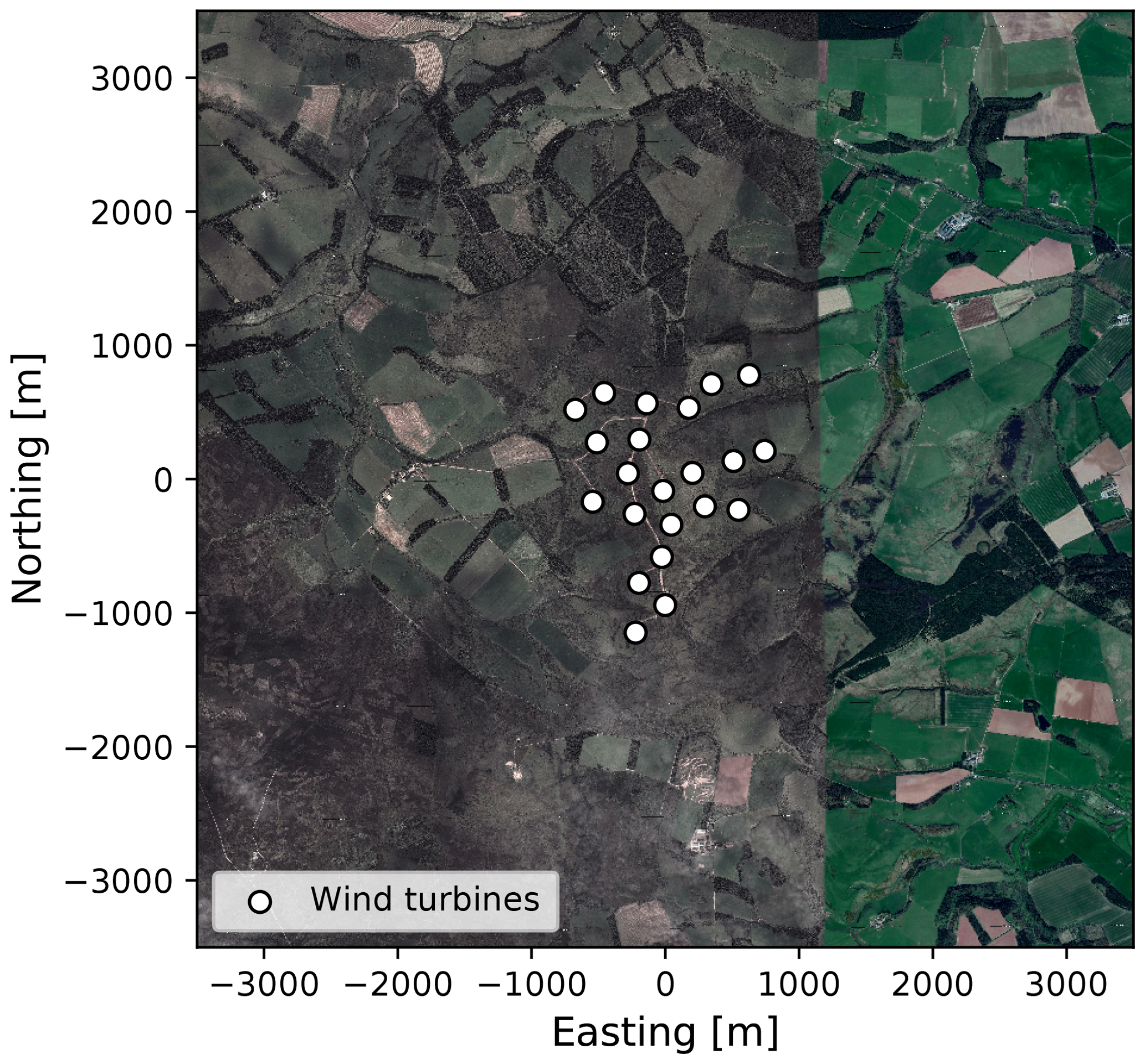
Figure 5 The aerial image of the Scottish site. Aerial data: © Google Maps, DigitalGlobe.

Due to the compact design of the wind farm, we decided to skip the measurement position optimization and try to generate a measurement campaign in which we intend to measure at every wind turbine position. Considering that the site is relatively close to the coast, surrounded by agricultural land and the altitude is about 300 m a.s.l., thus relatively low, the site should experience a good concentration of aerosols. Nevertheless, we cannot expect that the WindScanner lidars will have a 6 km range all the time and assume that on average the WindScanner lidars would have a range of at least 3 km at the selected site (i.e., half of the maximum claimed range). This estimation is based on our experience in doing measurement campaigns at various locations and in different atmospheric conditions.

Using this range together with the map extent, campaign-planning-tool outputs the combined layer (see top image in Fig. 6). The dark red colored areas show positions from where an individual scanning lidar can reach out to all measurement positions. Those areas are relatively large because the wind farm layout is compact. For this example, we chose to place the first WindScanner at the south of the wind farm (coordinates of 400, −1600 and 350 m in easting, northing and altitude a.s.l., respectively, relative to the map center coordinates of 535 662, 6 183 892 m in easting and northing, UTM zone 30U).

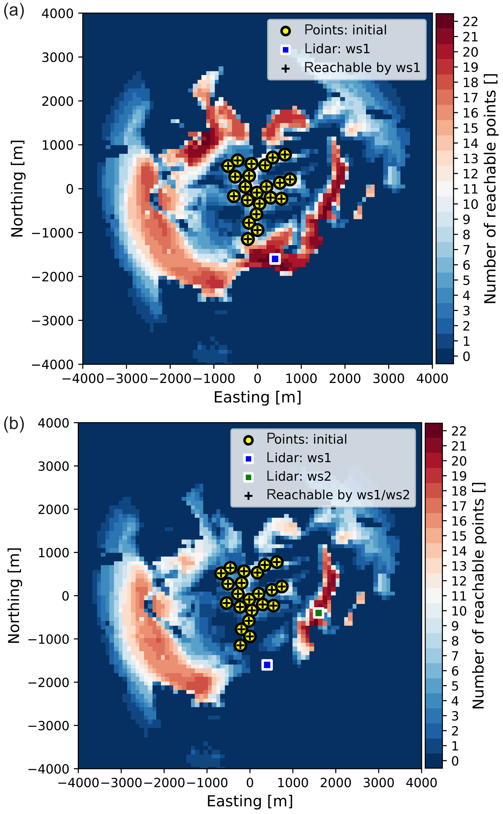
Figure 6 Placing lidars at the Scottish site: (a) locating first lidar at the combined layer; (b) locating second lidar at the second lidar placement layer.

As explained in Sect. 2 (Phase 3), the first lidar placement is instrumental for the second lidar placement because of the intersecting angle between the respective lidars' beams. There is only one area of the map where the placement of the second lidar assures that all measurement points are within reach and measurable with fair accuracy (bottom image in Fig. 6). By selecting the position of the second lidar (coordinates of 1600, −400 and 304 m in easting, northing and altitude a.s.l., respectively, relative to the map center coordinates), we complete the generation of one measurement campaign layout. In practice, we would generate several layouts (for different positions of WindScanner 1 and WindScanner 2) and assess their feasibility by inspecting aerial images, e.g., looking for access roads and nearby power lines or houses. However, for the sake of demonstrating the workflow, we have generated only a single layout.

Since we have both the measurement and lidar positions, we have all the elements to optimize and generate the trajectory. Figure 7 shows the optimum trajectory through the measurement points, resulting from the modified TSP (see Sect. 2 – Phase 4).

Figure 7 Final campaign design at Scottish site.

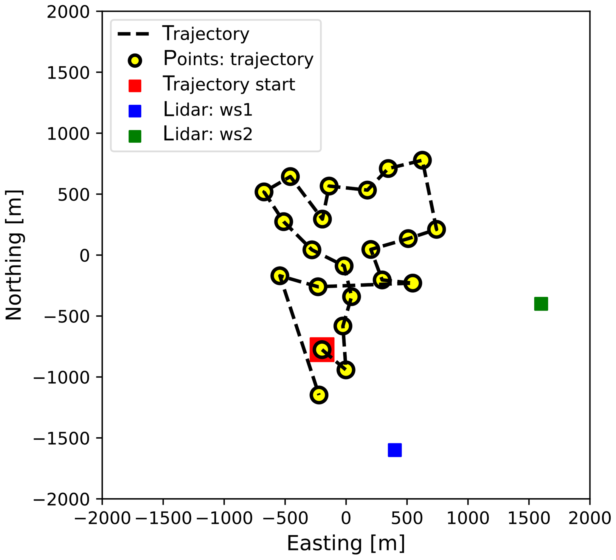
Considering the kinematic limits of the scanner head and that we are performing step-stare scans, we can apply the elevator kinematic problem on the trajectory points. This step yields the required time to move the scanner heads from one point of the trajectory to another, which in our case is about 14 s for the entire trajectory with an additional 22 s for measurements. Overall, one complete scan of all measurement points will take about 36 s, which results in about 16 samples of each measurement point per 10 min period. Typically we aim at having at least 10 samples per 10 min period which is satisfied with this configuration.

To verify that the optimized trajectory indeed takes the least amount of time, we have calculated the motion time for 10⁶ trajectory configurations by randomizing the order of trajectory points. This is a fraction of all possible permutations of trajectory points ($P_{n=\mathrm{22}}=\mathrm{22}\mathrm{!}$). However, since the order of points is randomized (thus not correlated) the results shown in Fig. 8 are trustworthy. Based on the derived results, the optimized trajectory is on average 8 s shorter for this specific campaign layout (i.e., the position of measurement points and lidars).

Figure 8 A histogram of motion time for 10⁶ different trajectory configurations for the Scottish site. The min, mean, max and standard deviation are 17.15, 22.09, 25.76 and 1.03 s, respectively.

One way to gauge the value of a WindScanner campaign is to estimate how much the uncertainty of the annual energy production (AEP) is reduced compared to a single met mast campaign. Since the flow model can account for a large part of the total uncertainty in complex terrain, a reduction in the extrapolation distance (i.e., a distance between a turbine and measurement position) gives a reduced flow model uncertainty. A method for estimating the flow model uncertainty has been published by Clerc et al. (2012). In the paper, the part of the extrapolation uncertainty associated with the distance is proposed to be

$$\begin{array}{}\text{(25)}& u_d=\mathit{\lambda }\left(\mathrm{1}-e^{-d/L}\right),\end{array}$$

where λ=10 %, L=1 km and d is the extrapolation distance.

We will consider a single centrally placed met mast and calculate an average ${\stackrel{\mathrm{‾}}{u}}_{d_{\mathrm{mast}}}$ taking into account all turbine positions. Based on Eq. (25) we have calculated ${\stackrel{\mathrm{‾}}{u}}_{d_{\mathrm{mast}}}$ to be 4.3 %. Since the derived WindScanner setup allows for measurements at every turbine location, the extrapolation uncertainty for the multilidar campaign will be 0 %. To reproduce the previous results, consult the Jupyter Notebook file in Vasiljević and Bechmann (2019b).

3.3 Site 2 – Italy

The Italian wind farm consists of 36 wind turbines with a 78 m hub height. The turbines are distributed over a large area (see Fig. 9) but somewhat clustered in small groups (Fig. 10) often with interturbine distances of less than 300 m (3 rotor diameters). With a coastline only 10 km to the west, a complex coastal–inland wind climate transition is expected to occur across the wind farm. The terrain has an average 7 % slope from the coast to the wind farm. The wind farm is surrounded by farmland; although, in a range of about 7 km there are several medium-sized towns that are forming an urban area ring around the farm site.

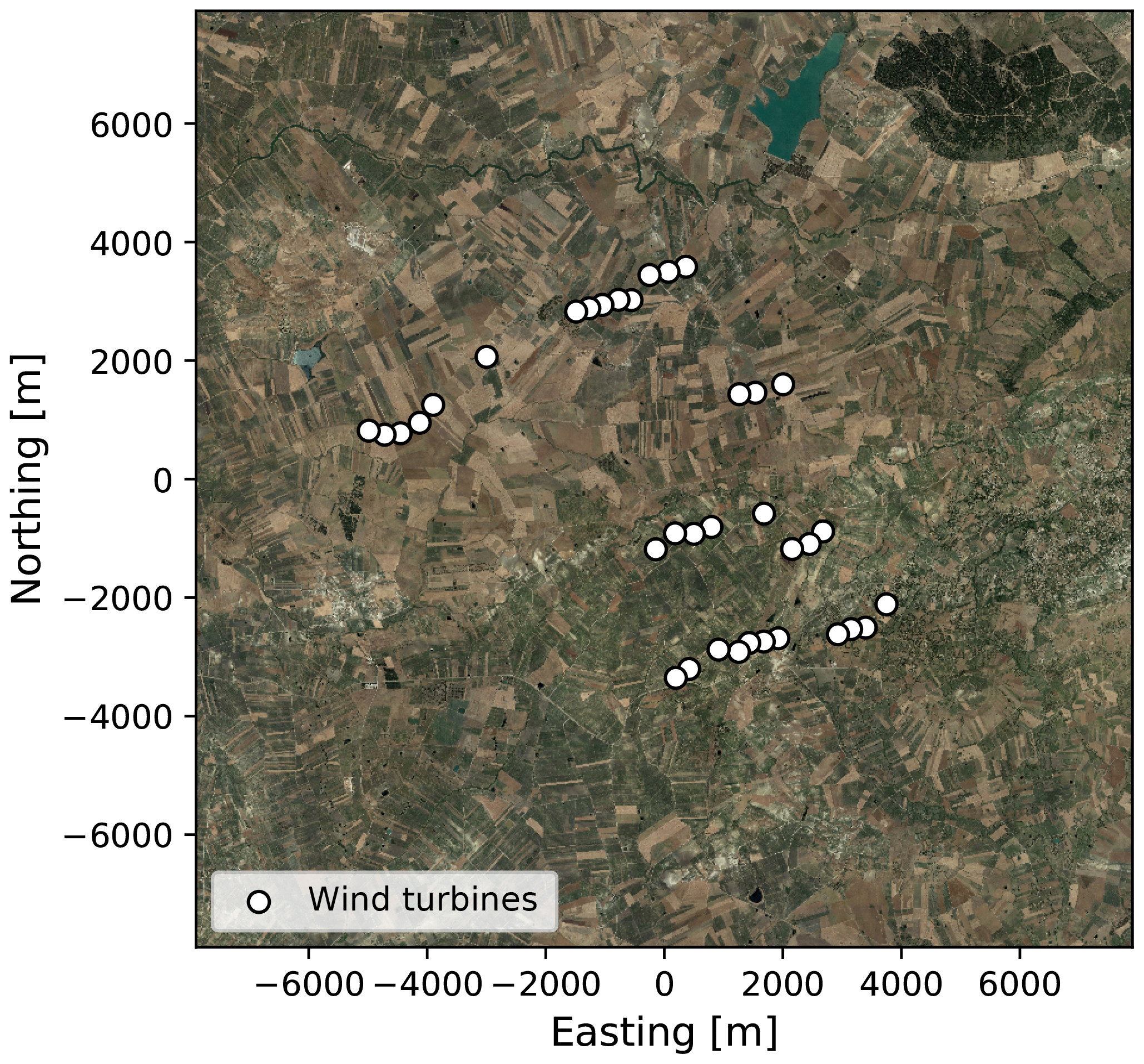
Figure 9 The aerial image of the Italian site. Aerial data: © Google Maps, DigitalGlobe.

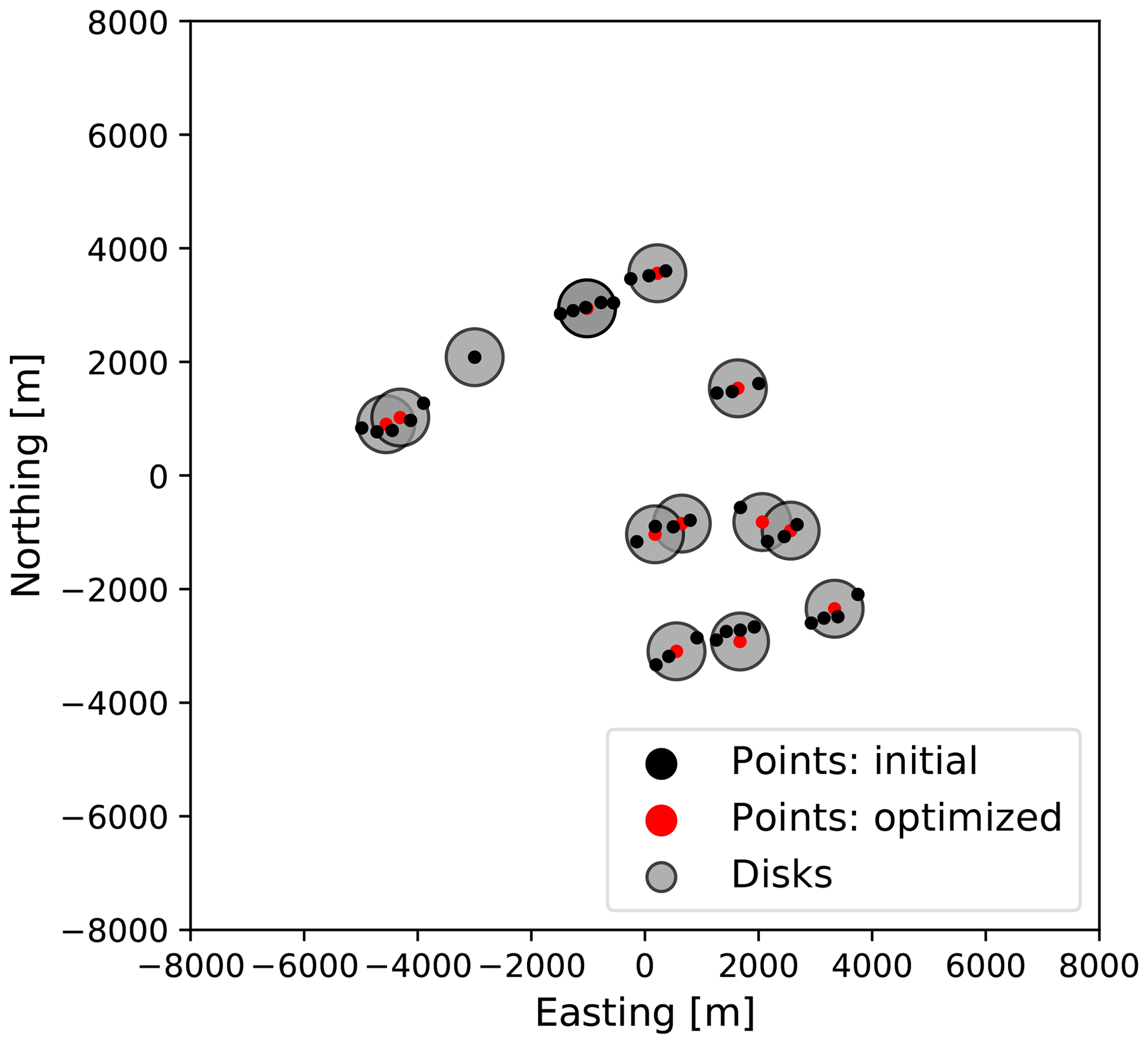
Figure 10 Measurement locations for Italian site: black dots – wind turbine positions, gray circles – disks covering wind turbine positions, red dots – optimized measurement positions (i.e., disk centers).

Given the specific layout of the wind farm, having more or less isolated groups of tightly packed wind turbines, we decided to apply the measurement point optimization. For this wind farm, the representativeness radius was set to 500 m, which is 4 times smaller than the maximum suggested value for the complex terrain sites (MEASNET, 2016). With this conservative setting, the optimization routine found 13 disks of radius equal to 500 m which covers all 36 wind turbine locations (Fig. 10). The disk centers represent measurement positions.

From there, the workflow was applied in the same way as it was for the Scottish site. In comparison to the Scottish site, the Italian wind farm is even closer to the sea, and it is surrounded by an urban area that in our experience increases the aerosol concentration resulting in an improved lidar range. Therefore, for the Italian site, we can expect to have an average measurement range of 4 km for the WindScanner systems. The combined layer generated using campaign-planning-tool is shown as the top image in Fig. 11. For this site, there are no positions from which any lidar can reach all 13 measurement positions. At best, there are only a few locations from which one lidar can reach 11 out of 13 measurement points. The top image of Fig. 11 shows the selected location for the first lidar installation (coordinates of −1254, −766 and 253 m northing, easting and height a.s.l., respectively, relative to the map center coordinates of 297 200 and 4 189 947 m in northing and easting, respectively, UTM zone 33S). The layer for the second lidar placement (the bottom image in Fig. 11) shows that the second lidar can reach nine measurement positions (not necessarily coinciding with those reachable by the first lidar) at most and this can only be achieved from a few locations. Of these locations, we selected one which assures that we cover the largest extent of the wind farm, thus getting good spatial information on the farm wind resources. The coordinates of a selected location for the second lidar are 1700, 100 and 299 m in northing, easting and height a.s.l. relative to the map center coordinates (the bottom image in Fig. 11).

Figure 11 Placing lidars at Italian site: (a) locating first lidar at the combined layer; (b) locating second lidar at the second lidar placement layer.

Considering the positions of WindScanner systems, reachable measurement points and kinematic limits, we derived an optimum trajectory through the measurement points and calculated the timing for the synchronized scanner head motion (Fig. 12). Based on the calculated timing for the scanner heads motion and considering one second accumulation time per measurement point, one scan through all the points takes roughly 20 s of which 8 s are spent on measurements (consult Jupyter Notebook file in Vasiljević and Bechmann, 2019c). This provides us with about 30 measurement samples at each measurement point within a 10 min period.

Figure 12 Final campaign design for Italian site.

To verify that the optimized trajectory is indeed the shortest in duration, we have generated all possible trajectories by making permutations of trajectory points. Unlike for the Scottish site, for the Italian site this is feasible since the trajectory contains only eight measurement points, thus there is 40 320 (8!) unique trajectories. For each trajectory, we have calculated the total motion time considering that the lidars will be operated in sync. The results are shown in Fig. 13. Based on the derived results the optimized trajectory is on average 6 s shorter for this specific campaign layout (i.e., the position of measurement points and lidars).

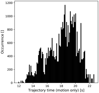
Figure 13 A histogram of motion time for 40 320 different trajectory configurations for the Italian site. The min, mean, max and standard deviation are 11.93, 18.14, 22.66 and 2.1 s, respectively.

Like in the previous example we will calculate the averaged extrapolation uncertainty considering a single centrally placed met mast (${\stackrel{\mathrm{‾}}{u}}_{d_{\mathrm{mast}}}$). The derived value for ${\stackrel{\mathrm{‾}}{u}}_{d_{\mathrm{mast}}}$ is 9.21 %. Unlike the previous example where we were able to measure at every turbine location, the current WindScanner layout is not able to provide the equivalent measurements. Therefore, even the WindScanner measurement campaign will have extrapolation uncertainty. To derive the extrapolation uncertainty for the WindScanner campaign (${\stackrel{\mathrm{‾}}{u}}_{d_{\text{dual-Doppler}}}$), we will treat the WindScanner campaign as a multimast campaign, and when calculating distance d for Eq. (25) we will use the closest measurement point to a wind turbine location. Based on this setup the derived value for ${\stackrel{\mathrm{‾}}{u}}_{d_{\text{dual-Doppler}}}$ is equal to 4.61 %. To reproduce these results, consult the Jupyter Notebook file in Vasiljević and Bechmann (2019c).

3.4 Site 3 – Turkey

The Turkish wind farm consists of 22 wind turbines with an 80 m hub height. The wind farm extends 8 km from north to south (see Fig. 14) with the three most northerly turbines separated by about 2 km from the rest. The interturbine distance is 400–500 m (4–5 rotor diameters) for most turbines. The turbines are located along a 1600 m tall north–south ridge and the main wind direction is from the northeast (i.e., perpendicular to the ridge line). In the main wind direction, the mean terrain slopes are about 12 % and with extremes reaching 50 % the site should be regarded as very complex. The land cover is sparse vegetation with a patch of forest along the western-facing slopes.

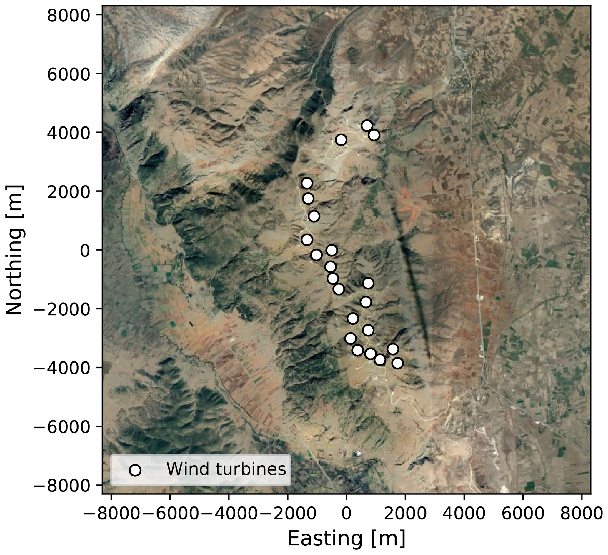
Figure 14 The aerial image of the Turkish site. Aerial data: © Google Maps, DigitalGlobe.

For this site, we assumed the average lidar measurement range to be 3 km, and we used the representativeness radius of 400 m. Our assumption on the average range in the case of the Turkish site is probably closer to what a lidar would probably achieve in a field operation (thus less conservative) due to operation in high altitude where we usually experience low aerosol concentration and often low clouds and fog. On the other hand, the selected representative radius is 100 m lower than in the case of the Italian site, thus about 5 times smaller than the recommended value by MEASNET. Running the workflow using these parameters we generate a measurement layout with 10 measurement positions (see Fig. 15) with the associated combined layer for the first lidar placement shown in Fig. 16, top image.

Figure 15 Measurement locations for the Turkish site: black dots – wind turbine positions, gray circles – disks covering wind turbine positions, red dots – optimized measurement positions (i.e., disk centers).

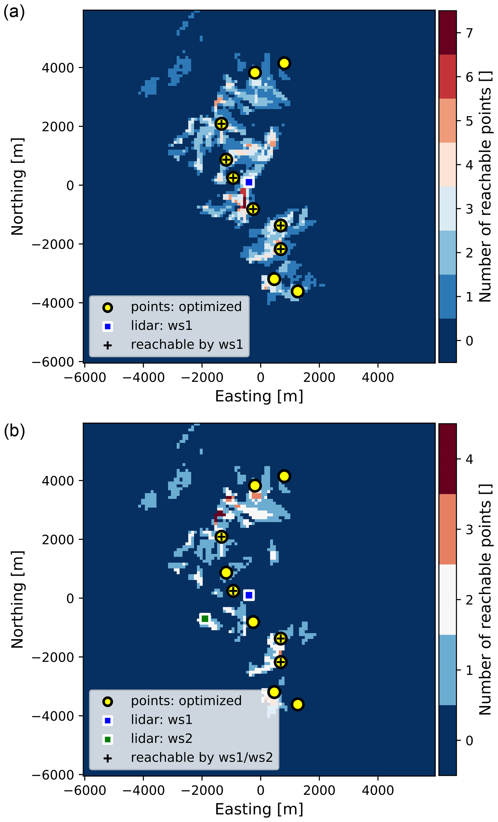
Figure 16 Placing lidars at the Turkish site: (a) locating first lidar at the combined layer; (b) locating second lidar at the second lidar placement layer.

There are only a few good locations for placing the two lidars, due to the wind farm length (8 km) and the lidar average range (3 km). Once again the best solution is to place the lidars in the middle of the wind farm. The top image of Fig. 16 shows the first lidar placement, whose coordinates are −400, 100 and 1562 m in northing, easting and height a.s.l., respectively, relative to the map center coordinates (easting 249 672 m and northing 4 227 405 m, UTM zone 36S).

Knowing the first lidar position leads us to the generation of the second lidar placement layers. From the bottom image in Fig. 16 there is hardly any area where the second lidar could be placed. Also, the bottom image in Fig. 16 shows the result of our choice for the second lidar placement (second lidar coordinates are −1900, −700 and 1492 m in northing, easting and height a.s.l. relative to the map center).

The designed WindScanner layout can provide measurements in 4 out of 10 measurement points that cover the middle part of the wind farm (Fig. 17). There are two measurement points in the middle of the farm that are not reachable since the beam of the second WindScanner is blocked by the hill crest. Also, the upper and lower quarters of the wind farm area are not reachable with the current layout. In principle, we would probably need two or more WindScanner systems to cover the entire wind farm (i.e., four scanning lidars).

Figure 17 Final campaign layout for Turkish site.

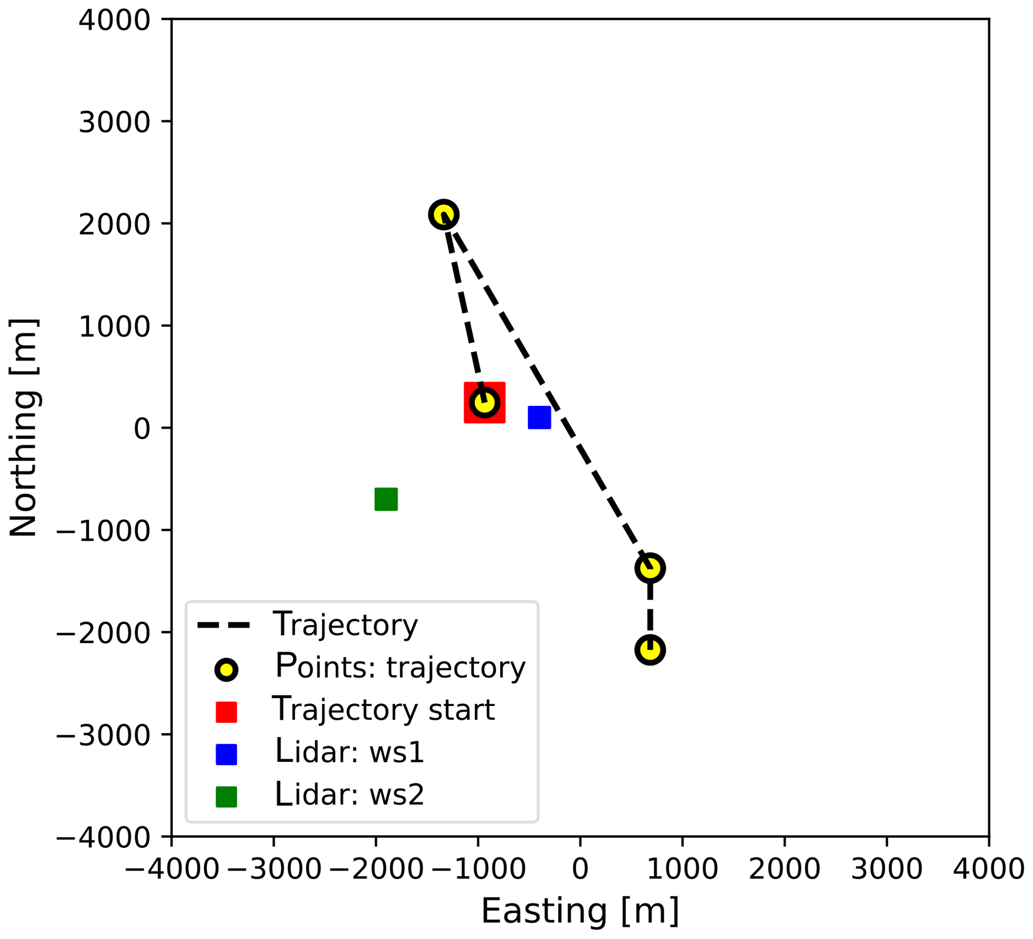
Considering the WindScanner systems and measurement locations together with the kinematic limits as the input for the last phase of the workflow we reach the optimized trajectory. The trajectory total time is 13.26 s of which 4 s are spent on the wind speed measurements. This trajectory would provide about 43 samples of each measurement point within a 10 min period. Similar to the Italian site, to verify that the optimized trajectory is the shortest one, all possible trajectories have been generated (the total of 4!=24). Considering all possible trajectories, the average trajectory time (motion part only) is 11.13 s, with a standard deviation of 2.34 s. The minimum and maximum time is 9.26 and 14.42 s, respectively. To reproduce these results, consult the Jupyter Notebook file in Vasiljević and Bechmann (2019d).

We will repeat the same analysis of the extrapolation uncertainty as in the case of the previous sites. Considering a single centrally placed met mast the average extrapolation uncertainty ${\stackrel{\mathrm{‾}}{u}}_{d_{\mathrm{mast}}}$ it is equal to 8.41 %, while in the case of the WindScanner campaign ${\stackrel{\mathrm{‾}}{u}}_{d_{\text{dual-Doppler}}}$ is equal to 5.69 %. To reproduce these results, consult the Jupyter Notebook file in Vasiljević and Bechmann (2019d).

4 Discussion

4.1 Discussing results

The primary purpose of the described workflow is to design dual-Doppler measurement campaigns for wind resource assessment (WRA). This scope follows the RECAST project ambition which is focused on developing a new way of performing WRA based on multiple measurement points using WindScanner systems. This has driven the choice of examples for Sect. 3 of this paper. However, the workflow and its digitalized version (i.e., campaign-planning-tool) described in this paper are not limited to only planning WRA campaigns. It can be used to design any campaign using one or several scanning lidars. It can easily be applied to any type of scanning lidar since it only requires lidar specifications, which are expected lidar range and scanner head kinematic limits (i.e., maximum acceleration and speed).

Planning the measurement campaign thoroughly especially with such complex instruments as scanning lidars ensures higher data availability during the campaign and eventually saves time and money. Lidars are very mobile and allow agile measurement campaigns compared to a met mast, but too often the ease of deployment is mistaken with a limited (underestimated) need of planning. This study provides solutions for optimizing measurement points, lidar positions and measurement trajectory which represent a necessary foundation for accurate measurements of wind resources over the wind farm site. We have demonstrated that the above-stated optimization leads to reduced trajectory timing and thus an increase in the sampling rate.

The point of the workflow and the corresponding Python package is also to carefully consider the relevance of using scanning lidars for a measurement campaign. We have shown that for large sites one set of two WindScanner systems cannot measure over the whole wind farm area. This is very important to realize at the campaign planning stage when there is still time to either give priority to one part of the site or consider using a second set of two WindScanner systems to cover the rest of the site.

Nevertheless, with a rather simplified approach in the assessment of the AEP uncertainty, we have shown that even when WindScanner systems cannot cover the entire site, still a reasonable reduction of the uncertainty should be expected. Specifically, based on the presented examples, using multilidars and optimizing measurement and lidar positions on average the horizontal extrapolation contribution to the AEP uncertainty can be reduced from 2 % to 5 % compared to a single mast campaign.

4.2 Improving workflow

The presented workflow can already solve many important challenges regarding the scanning lidar deployment. Nevertheless, we envisage a further development of the workflow and thus the Python package campaign-planning-tool.

In the current application of the workflow, we were predicting the lidar range based on our experience. We plan to develop a Python package that will be able to predict the lidar range using external databases of global atmospheric visibility for a given site. In the mean time, our suggestion when planning the lidar campaign is to generate campaign layouts considering a conservative approach in which the expected range of the lidar should be in the range from 75 % to 50 % of the claimed range by the lidar manufacturers. Directly connected to the range prediction is the development of a Python package which will be able to predict the lidar data availability at any desired range during the planned measurement period taking into account, for example, the cloud height, fog or mist occurrence from the Weather Research and Forecasting (WRF) model.

Furthermore, the proposed approach in optimizing measurement positions will be extended by considering other criteria for finding measurement positions apart from the representativeness radius. These are, for example, terrain elevation, speed-up factors, roughness changes, local obstacles, etc. In principle, we will strive to incorporate as many factors as possible that can cause local changes in the flow. In other words, the optimization of measurement positions will consider drivers of flow model uncertainty when finding measurement positions.

Finally, eye safety has not been considered in the presented workflow. In the next iteration of the workflow, we will incorporate these issues as yet another restriction zone (GIS) layer for the placement of lidars.

5 Conclusions

This paper provides an exhaustive description of a workflow for planning and configuring scanning lidar measurement campaigns. The purpose is to find the most suitable measurement positions (considering a preliminary wind farm layout), survey scanning lidar placements considering lidar and site constraints to secure accurate measurements, and optimize scanning lidar trajectory to boost the number of measurement samples. The presented workflow can help to avoid many pitfalls that can be predicted before the start of the campaign, limiting the risks to the campaign itself. The workflow, in its digitalized version, has been demonstrated for planning campaigns for resource assessment for three different sites. For a small wind farm layout, a dual-Doppler system could be positioned such that measurements could be made at all turbine positions. For the other larger sites, the number of measurement points had to be optimized and a set of two lidars could only cover some parts of the sites. Nevertheless, for all examples, we have demonstrated that using the proposed workflow a significant reduction of the trajectory timing and AEP uncertainty are achievable.